Field-temperature phase diagram of the enigmatic Nd2(Zr1-xTix)2O7 pyrochlore magnets
Abstract
By combining neutron scattering and magnetization measurements down to 80 mK, we determine the phase diagram of the Nd2(Zr1-xTix)2O7 pyrochlore magnet compounds. In those samples, Zr is partially substituted by Ti, hence tuning the exchange parameters and testing the robustness of the various phases. In all samples, the ground state remains “all in / all out”, while the field induces phase transitions towards new states characterized by “2 in – 2 out” or “1 out – 3 in / 1 in – 3 out” configurations. These transitions manifest as metamagnetic singularities in the magnetization vs field measurements. Strikingly, it is found that moderate substitution reinforces the stability of the “all in / all out” phase: the Néel temperature, the metamagnetic fields along with the ordered magnetic moment are higher in substituted samples with 10%.
I Introduction
The last decades of research in the field of condensed matter have seen the emergence of a rich and new physics, going beyond the Néel paradigm and transcending conventional descriptions based on Landau’s theory. Frustrated magnetism has largely contributed to these developments, pointing to the existence of new states of matter, such as spin liquids or Coulomb phases. The interest in these states originates from the fact that they host fractional excitations, are described by emergent gauge fields and exhibit large-scale quantum entanglement [1, 2, 3].
The pyrochlore network, built from tetrahedra joined by their vertices has played a key role in this field. In particular, Ising spins located at the summits of these tetrahedra and coupled by ferromagnetic interactions form an unconventional state called spin ice [4]. The spins remain disordered, but nevertheless obey a local rule known as the “2 in – 2 out” rule, which stipulates that each tetrahedron must have two incoming and two outgoing spins, in close analogy with the disorder of hydrogen atoms in water ice. It results in a residual entropy at zero temperature [5], as well as in a peculiar local organization of the spins. The latter can be observed by neutron scattering, and manifests as an elastic pattern in reciprocal space with bow tie singularities also called pinch points [6, 7, 8]. Furthermore, the ice rule can be interpreted as the zero divergence condition of an emergent magnetic field (), a mapping that has allowed considerable theoretical development.
In most of the pyrochlore materials of interest today, the spin is due to the 4f magnetic moment of a rare-earth. These compounds have been abundantly investigated in the literature [3], with the description of a large variety of ground states arising from the interplay between magnetic exchange couplings, dipolar interactions, and single-ion anisotropy of the magnetic moment. It is worth mentioning spin ices, but also spin liquids, fragmented states and apparently more conventional magnets.
Among them, Nd2Zr2O7 has attracted much attention. As inferred from a positive Curie-Weiss temperature, indicating ferromagnetic interactions, and combined with an Ising anisotropy, a spin ice ground state is expected in this material [9, 10]. Indeed, the expected pinch point pattern is observed below K [11]. Upon further cooling, however, the spin ice state gives way to an “all in / all out” (AIAO) ground state, with all the spins pointing out or into each tetrahedron, hence highlighting dominant antiferromagnetic interactions [9, 10, 12].
Motivated by this very rich physics and by the competition between spin ice and AIAO state [13, 14], we investigate in this paper the field - temperature phase diagram of this material. Moreover, as documented in many pyrochlore compounds such as Tb2Ti2O7 [15], Er2Ti2O7 [16] or Yb2Ti2O7 [17], weak substitution, often less than 5%, can change the physical properties leading to a quick collapse of the ground state. With this in view, the study was extended to the Nd2(Zr1-xTix)2O7 family, using two nominal compositions and . These investigations yield a systematic and comprehensive survey of the phase diagram for magnetic fields applied along the three main high symmetry directions (, and ) of the pyrochlore lattice.
The paper is organized as follows. In section II, we introduce the main properties of Nd2Zr2O7 and the context of the study. In section III and IV, we present the experimental methods and determination of the phase diagrams for the three studied samples and the three field directions. Finally, by comparing these results with mean-field calculations, we discuss in section V the involved field induced processes, including the role of domains and metastable states, and address the impact of Ti substitution on the phase diagram.
II Experimental background and interpretations : a short review
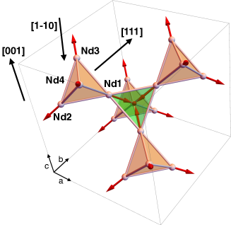
Using a combination of magnetization, elastic and inelastic neutron scattering measurements [9, 11], previous investigations of Nd2Zr2O7 have shown that the Nd3+ magnetic moments exhibit a strong Ising anisotropy along local 111 axes, together with a dipolar-octupolar nature [18], different from the standard Kramers doublets studied so far. Furthermore, neutron diffraction has shown that the AIAO antiferromagnetic state (Figure 1) is characterized by a strongly reduced ordered moment [9, 10, 19], and coexists with a pinch point pattern typical of spin ice. Nevertheless, inelastic neutron scattering clearly pointed out that, at low temperature, this pattern is not an elastic feature as in classical spin ice, yet is dynamic, shifted to finite energy by an energy eV, and that was hence called a dynamical spin ice mode [11]. In other terms, the peculiar AIAO order of Nd2Zr2O7 appears to be protected by a “gap” from spin ice. In addition, the spin excitation spectrum revealed by inelastic neutron scattering also encompasses well resolved dispersing features akin to spin wave branches. These experimental results suggested that quantum effects are at play.
Concomitantly, theoretical studies highlighting the dipolar-octupolar nature of the Nd3+ ion [18] have shown that the relevant variable is a pseudo spin ( defined in the local ion frame) and which resides on the pyrochlore lattice sites. The magnetic moment , hence the observable quantity, essentially identifies with the component of this pseudo spin and is carried by the local axes, consistent with the observed Ising nature of the Nd3+ ion. The and components identify with octupolar moments of the 4f electronic distribution and are thus barely visible to neutrons 111A weak contribution to the neutron scattering cross section is expected at large wavevectors, but importantly the component transforms like a dipole and thus can be coupled to the component. The low energy properties are then governed by:
which, after a rotation in spin space by an angle , can be recast in the XYZ Hamiltonian [18, 12]:
| (1) |
and where the rotation away from the axis defines the new components and the new coupling constants . According to the most recent investigations [21, 14], the parameters yielding an accurate description of the spin dynamics are K and close to zero. The corresponding ground state is an AIAO state with the magnetic moments aligned along the directions, as proposed in Ref. [12]. It is worth noting that the ordered pseudo spin is close to its full value . The tilted angle rad is estimated from the Curie-Weiss constant, or from the observed ordered moment. Indeed, the projection of the ordered moment back to the original axes introduces a factor of , hence providing a simple explanation for the experimental observation of an AIAO state with a reduced magnetic moment.
In this work, we combine neutron diffraction and magnetization measurements to explore the evolution of the AIAO magnetic configuration as a function of temperature and magnetic field applied along the three high symmetry directions, and in the presence of non-magnetic Ti substitution at the B-site of the pyrochlore lattice. This study thus envisages the effect of a Zeeman term added to the XYZ Hamiltonian (1):
| (2) | ||||
are the local directions and is the anisotropic factor, estimated to 4.8 in the pure compound and 5 in the 2.5 and 10 % Ti substituted samples. In addition to classical parameters like Curie-Weiss, effective moment and Néel temperature, the detailed analysis of the vs curves highlights significant field induced processes, like metamagnetic transitions, that are further analyzed by means of neutron diffraction. This methodology allows one to determine in a systematic way how the microscopic magnetic structure evolution is related to the changes that occur at a more macroscopic scale.
It is worth noting that, as described above, the measured ordered component in zero field is only a fraction of the total magnetic moment of the Nd3+ ion () (See Table 2). Nevertheless, in the presence of a magnetic field, the pseudo spins tilt towards the local directions, so that the measured ordered moment (which is only the component) recovered in high field corresponds to the total magnetic moment.
III Methods
III.1 Samples
Nd2(Zr1-xTix)2O7 samples (with and ) were prepared at the University of Warwick in polycrystalline form by standard solid-state chemistry methods, using Nd2O3, ZrO2 and TiO2 as starting reagents [22, 23]. To ensure the appropriate composition of the final compounds, the Nd2O3 powder was pre-heated in air at C for 24 hours. Powders of the starting oxides were weighed in stoichiometric amounts, mixed together, pressed into pellets and then heat treated in air for several days (in three or fours steps) at temperatures in the range C. The annealed pellets were reground between each step of the synthesis to ensure good homogeneity and to facilitate the chemical reaction. Powder X-ray diffraction measurements confirmed the phase purity of the synthesized Nd2(Zr1-xTix)2O7 polycrystalline samples.
Single crystals of the two Ti-substituted samples were grown from the polycrystalline samples by the floating-zone technique using a four-mirror xenon arc lamp optical image furnace [22, 23]. The 2.5 % substituted sample is a fragment of the single crystal used in Ref. 14.
Below, we report only on the single crystal properties. Powder sample properties are summarized in Appendix B.
III.2 Bulk magnetic measurements
Magnetization and AC susceptibility measurements were performed down to 80 mK on the single crystal samples using superconducting quantum interference device (SQUID) magnetometers, equipped with a dilution refrigerator developed at the Institut Néel-CNRS Grenoble [24]. The crystals were glued with GE varnish on a copper plate, and measurements were collected with the magnetic field aligned along the three high symmetry directions of the crystals (, or ). All the data shown below were corrected from demagnetizing field effects. Demagnetizing factors were estimated from the sample shapes using the Aharoni formula [25].
III.3 Neutron diffraction
Single crystal diffraction experiments were carried out at D23 (CRG CEA-ILL, France) using a wavelength Å and operated with a copper monochromator. The samples were glued on the Cu finger of a dilution insert and placed in a cryomagnet. The experiments were conducted with the (vertical) field either parallel to the , or high symmetry crystallographic direction. The three orientations were measured for the three samples, except for the 10 % substituted sample for which the condition could not be measured.
| Nd Atoms | ||||||
|---|---|---|---|---|---|---|
| Nd1 | 0.25 | 0.25 | 0.50 | 1 | 1 | -1 |
| Nd2 | 0.00 | 0.00 | 0.50 | -1 | -1 | -1 |
| Nd3 | 0.00 | 0.25 | 0.75 | -1 | 1 | 1 |
| Nd4 | 0.25 | 0.00 | 0.75 | 1 | -1 | 1 |
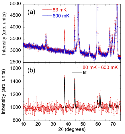
As we shall see later on, the magnetic structures have a propagation vector, hence magnetic and crystalline intensities occur on the same positions. A full data collection was thus first measured at K to serve as a reference of the crystalline intensities and refine the sample volume, the Ti content , the extinction parameters and atomic positions in the Fdm space group. Additional data collections (consisting in 80 Bragg peaks) were then measured at low temperature (80 mK), at selected fields ranging from T to T. The magnetic structure at each field was then refined with the Fullprof suite [26] using the difference between the low temperature and 6 K diffractogram intensities. Owing to the strong Ising character of the Nd3+ ions, the data have been analyzed assuming that the magnetic moments lie along the Ising axes (see Table 1). The sign, with respect to the convention given in Table 1 and the amplitude of the moments in a given tetrahedron are the free parameters of those fits.
In addition, the intensity of selected Bragg peaks was recorded while ramping the field back and forth from T to T ( T/min was the minimum sweeping speed) to obtain a “continuous” evolution vs field. The sample was first cooled down to 80 mK in zero field and the field dependence of the intensity was then measured after the application of a T field to saturate the sample (larger fields up to T were also used, but this makes no changes in the “low” field results). The detailed method for the analysis of these field sweeping measurements is given in Appendix C.
| Single crystal Sample | Ti concentration | O2 position | Lattice parameter | Ordered moment | |||
|---|---|---|---|---|---|---|---|
| [%] | [Å] | [mK] | [mK] | [] | [] | ||
| 0 | 285 | 195 | 2.45 | ||||
| 375 | 235 | 2.52 | |||||
| 325 | 220 | 2.50 |
IV Results
IV.1 Physical characterizations
The structural refinements from neutron diffraction data of the single crystals with the 2.5 and 10 % substitution concentration are in agreement with the pyrochlore structure. The lattice parameters are close to the pure compound one ( Å) and the 48f oxygen atoms are found at the position . Noteworthy, the value of the Ti content was refined thanks to the significant difference in the scattering length for the two elements Zr and Ti. It is found to be 2.4 and 7.9 % in the so-called 2.5 and 10 % Ti-substituted samples respectively (see Table 2).
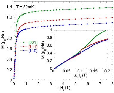
Isothermal magnetization curves for magnetic fields applied along the three high symmetry directions show three different saturated magnetizations (see Figure 2), in agreement with expectations in the case of Ising spins located at the vertices of the tetrahedra [27]. Curie-Weiss fits of the magnetization between and K give positive Curie-Weiss temperatures and effective moments of about for both Ti-substituted samples.
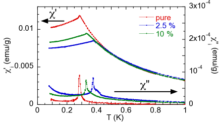
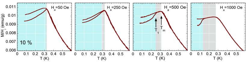
AC susceptibility measurements show a transition at low temperature in all compounds with a peak in both real and imaginary parts (see Figure 3). No frequency dependence of the peak position is observed between 0.057 and 570 Hz. Interestingly, the critical temperature reaches 376 mK for % and decreases back to 325 mK for %. Neutron diffraction measurements elucidate that the magnetic ground state is AIAO in the substituted samples with and for the 2.5 and 10 % substituted samples respectively. For both samples, the transition takes place at a higher temperature than in the pure compound ( mK) and with an ordered magnetic moment significantly larger (0.8 in the pure compound), as summarized in Table 2. It should be noted that these and ordered moment values for the substituted samples are nevertheless smaller than the ones measured on the powder samples with the same composition (See Appendix B).
At low field and in all samples, the vs curves show an inflexion point (see the insert in Figure 2) for the three field directions, which is associated to metamagnetic like processes [9]. The corresponding characteristic field can be followed by tracking the maximum of the derivative vs of these magnetization curves for different temperatures in order to build the phase diagram. In the following sections, the nature of the phases is investigated based on neutron diffraction data.
IV.2 Magnetic field along
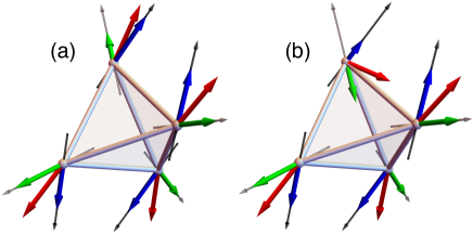
When applying a magnetic field along the direction, the AIAO ground state is expected to evolve towards an ordered spin ice state, with two incoming and two outgoing spins per tetrahedron and a net magnetization along the direction. According to symmetry, the 4 spins in a given tetrahedron form two subgroups consisting in spins (1,2) and (3,4) (see Figure 1). To follow the magnetic structure and figure out how the ordered spin ice configuration grows to the detriment of the “all in / all out” one, it is thus convenient to parametrize the magnetic moments as:
| (3) |
which corresponds to the sum of a generalized “all in / all out” component and of a “2 in – 2 out” component . By convention, considering a red tetrahedron of Figure 1, is positive (negative) when all the Nd magnetic moments are “out” (“in”), and is positive when Nd1 and Nd2 are “in” while Nd3 and Nd4 are “out” (2I2O configuration) and negative when Nd1 and Nd2 are “out” while Nd3 and Nd4 are “in” (2O2I configuration).
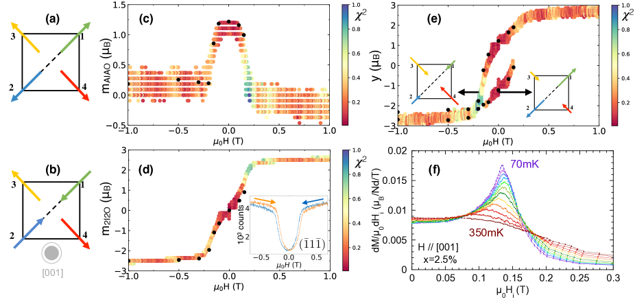
The Fullprof refinements highlight this field induced behavior, as shown in Figure 4 for the 2.5 % substituted sample. Starting from T, red tetrahedra of Figure 1 are in the 2O2I configuration with a net moment along . Upon increasing field, this “2 in – 2 out” component remains stable (decreasing smoothly) up to a field threshold from which it is suppressed to the benefit of the AIAO component, as shown in the panels (c) and (d) of Figure 4. This characteristic field is clearly observed when measuring the intensity of the reflection as a function of field, as shown in the inset of Figure 4(d).
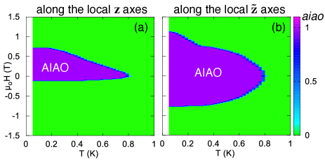
The AIAO component is maximum in zero field. It decreases when further increasing the field, while rises continuously, until reaching a value close to the saturation at the opposite of the first threshold field, i.e. when the AIAO component comes back to zero. This clearly separates two regions in the phase diagram: above a characteristic field , only a 2I2O component is present, while below, it coexists with an AIAO one.
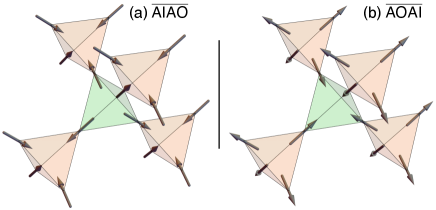
The analysis nevertheless points to two different situations upon increasing field from the 2O2I configuration: (i) either Nd1 and Nd2 flip, so that the Figure 1 red tetrahedra become “all in” (and green tetrahedra become “all out”), or (ii) Nd3 and Nd4 flip, so that the red tetrahedra become “all out”. These two magnetization processes lead to the formation of the two domains of the AIAO state, so-called or (See Figure 5), which cannot be distinguished in neutron diffraction measurements. The two domains have the same energy in the presence of the field which suggests that both are present simultaneously. Interestingly, the resulting moment ( or in Equation 3) on a given atom is different depending on the sign of , and thus on which domain is stabilized. This manifests through the two branches shown in the panel (e) of Figure 4 representing the magnetic moment of the Nd3 atom. Finally, almost no hysteresis is observed in magnetization and neutron field sweeping measurements, which indicates that both domains are present and that the magnetization process takes place while remaining close to thermodynamic equilibrium.
The signature of in the magnetization curves vs field is an inflexion point, which appears as a broad peak in the vs field curves (see Figure 4(f)). At the lowest temperature (about 80 mK), , determined from the maximum of , varies from up to T depending on the sample composition (see Table 3). The values of as a function of temperature are plotted for the three samples on the phase diagram of Figure 8(a). As expected, goes to zero at the Néel temperature, confirming that it is characteristic of the disappearance of the AIAO structure. The temperature dependence of is qualitatively similar in the three samples. Interestingly, the lower the , the lower the . Consequently, the pure compound has the lowest and the 2.5 % Ti-substituted sample has the highest one.
IV.3 Magnetic field along
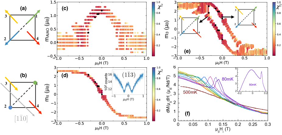
In the presence of a field, the situation is more complicated. In such a field direction, the system is usually described as two perpendicular chains, made of the spins 1 and 2 ( chains), and spins 3 and 4 respectively in our notations ( chain, see Figure 1). Spins 3 and 4 are almost collinear to the field and are thus expected to quickly reach saturation. In contrast, spins 1 and 2 have their Ising direction perpendicular to the field. The Zeeman effect is thus zero, yet the field indirectly affects their orientation via the coupling to the other spins [27]. To describe the magnetic structure as a function of field, the following parametrization was thus used:
| (4) |
It takes into account the “all in / all out” contribution (with the same sign convention as before) along with and which feature field polarized components parallel (for spins 3 and 4) and perpendicular to the nominal field direction (for spins 1 and 2).
Fullprof refinements of the neutron diffraction measurements highlight the saturation of the parallel spins in large magnetic fields: at T, the Nd3 and Nd4 moments reach , the Nd3 moment being “in”, and the Nd4 one “out” in positive field (see Figure 6(b)), and conversely in negative field. Noteworthy, they reach values as high as at T (see Figure 6(d)). At high field, the refined magnetic moment on sites 1 and 2 is found to be zero (or small 222It is worth mentioning that in a trial experiment where the field was not perfectly aligned along (about 4 degrees while less than 1 in the present experiment), such a non-zero moment could be refined, suggesting that it is likely a by product of the ill-aligned component of the field) (see Figure 6(c)). This confirms the disordered character of the (Nd1, Nd2) chains in applied field previously observed in Ref. 29. This study further reports diffuse scattering showing the existence of short-range correlations within the chains, that we could not address in the present work.
Neutron refinements (see Figure 6c) show that the AIAO component is suppressed upon increasing the field (in absolute values) at a critical value labeled . It is best observed when measuring the characteristic magnetic reflection as a function of the field, as shown in the inset of Figure 6(c).
Like in the case of the field, the analysis of the field sweeping measurements unveils two scenarii regarding the rise of the “all in / all out” component when starting from the high field state, and corresponding to the possible and domains. Indeed, considering the (Nd3, Nd4) chain in the saturated state, either the Nd3 or the Nd4 spin can flip to recover “all in” or “all out” configurations, with the same energy cost. It results in two possible branches in the total magnetic moment, as shown for the Nd3 atom in Figure 6(e).
The signature of in the magnetization curves vs field is characterized by a step-like anomaly and manifests as a little peak in the curves (see Figure 6(d)), which is more marked in the substituted samples than in the pure sample. Nevertheless, this peak is only clearly observed in positive field, when sweeping the field from negative values, as shown in the inset of Figure 6(d) at 80 mK. A small irreversibility is also observed on the reflection (not shown) in neutron diffraction measurements. These results imply that some kind of metastable states exist for this field direction, that we will address in more details in the discussion. The temperature dependence of is qualitatively similar in the three samples, and as for the direction, the pure compound has the lowest while the 2.5 % Ti-substituted sample has the highest one.
IV.4 Magnetic field along
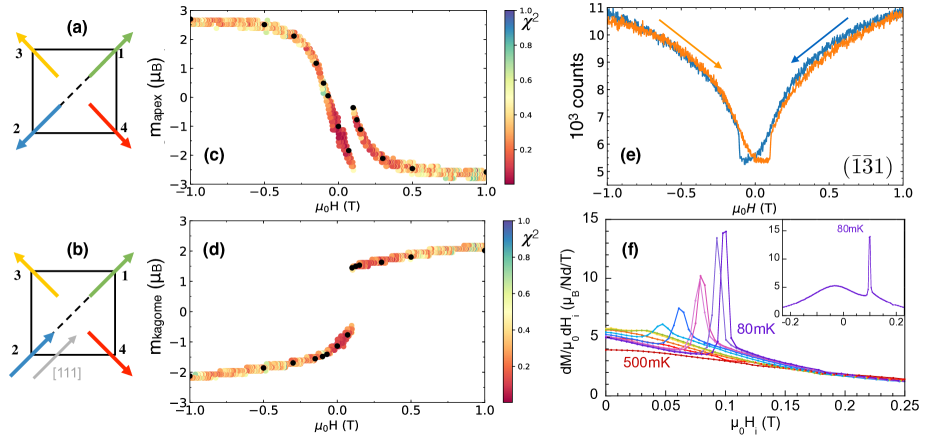
To discuss the case of a field applied along the direction, it is convenient to view the pyrochlore lattice as the stacking of triangular and kagomé planes. In a given tetrahedron, one shall then distinguish the apex spin, which is collinear to the field (Nd2), and three “kagomé” spins located in the kagomé layer (Nd1, 3 and 4), which experience the same Zeeman effect. The magnetic configuration is expected to go from a 1O3I to “all in” or “all out”, and eventually to 1I3O with increasing the field from up to T, a behavior described in the pure compound in Ref. [30, 19]. To describe this evolution, the following parametrization is used:
| (5) |
Neutron diffraction refinements reveal in both Ti-substituted samples the same singularity as the one already observed in the pure compound. It is characterized by a sudden jump for both the apex and the kagomé spins (see Figure 7(c,d)). At T, the kagomé spins are “in” while the apex is “out”, forming a 1O3I configuration. Upon increasing the field from T, the absolute value of the apex moment progressively decreases while the kagomé moments remain essentially unchanged. At some threshold T, the apex moment changes sign, and the structure becomes “all in”. This holds up to a critical field T where the kagomé moments abruptly flip while the apex moment nearly goes back to zero. Its amplitude increases then, but now follows a new magnetization process. The configuration has become 1I3O. The field is best observed when measuring the characteristic magnetic reflection as a function of the field, as shown in Figure 7(e).
The sharp transition at underlines the existence of metastable states when increasing the field, and which are again connected to the formation of either “all in” or “all out” configurations for the red tetrahedra, and thus to and domains. These domains are connected to the and configurations stabilized at large negative and positive fields respectively. Depending on the amplitude of the field, they become metastable, explaining the origin of the hysteresis clearly observed in the magnetization measurements displayed in the inset of Figure 7(f).
IV.5 Phase diagrams
| Sample | (T) | (T) | (T) |
|---|---|---|---|
| pure | 0.083 | 0.086 | 0.075 |
| 2.5 % | 0.135 | 0.162 | 0.111 |
| 10 % | 0.124 | 0.132 | 0.099 |
| Calculations | |||
| pure | 0.26 | 0.55 | 1.20 |
| 2.5 % | 0.32 | 0.72 | 1.13 |
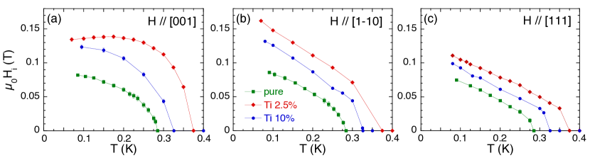
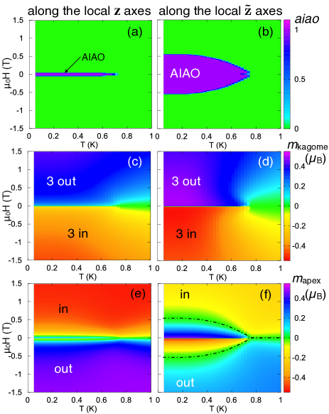
From the temperature dependence of the peak in the vs curves shown in the panels (f) of Figures 4, 6 and 7, we could construct the phase diagrams for the three field directions, and the three measured samples. They are displayed in Figure 8. The three samples show qualitatively the same behavior, the critical fields being related to the critical temperatures in all directions so that the larger the Néel temperature, the larger the critical field.
Along the and directions, the low field phase can be directly associated to an “all in / all out” phase, as demonstrated by the neutron diffraction results detailed in the above sections. Along , the critical fields seem to saturate at low temperature (and even to decrease slightly for the 2.5 % sample). On the contrary, the low temperature dependence of the critical field along does not show any sign of saturation.
The description in terms of AIAO component for the field along the direction is less relevant due to the different response of the apical and kagomé spins with respect to the field in that case. In addition, the observation of a very strong hysteresis suggests that the value of is unlikely an equilibrium value, as discussed in more details in Section V.
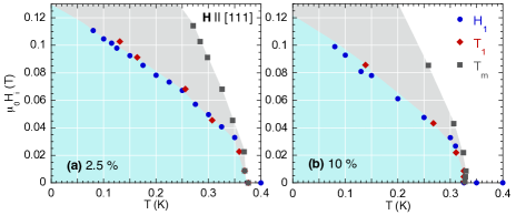
To further probe the nature of the field induced behavior in this field direction, we have performed vs measurements in various applied fields. In particular, field cooled (FC) experimental curves are expected to better approach the equilibrium state of the system. Zero field cooled - Field cooled (ZFC-FC) experiments were thus conducted at several applied fields between and Oe for the two substituted samples, as shown in Figure 9 for the 10 % sample. In low field (typically 100 Oe), both ZFC and FC curves show a maximum of the magnetization at a value labeled , which occurs roughly at the Néel temperature (determined from the AC susceptibility). However, a splitting between the ZFC and the FC curves is observed at lower temperature, below , with . As previously observed in the case of Nd2Hf2O7 [31], upon increasing the field, this ZFC - FC irreversibility moves to lower temperature, so that the ZFC-FC curves remain on top of each other in the temperature range .
The obtained characteristic temperatures and measured at a given applied field are plotted together with the maxima of vs measured at constant temperature in the phase diagram shown in Figure 10. Interestingly, the boundary defined by the points is found to coincide with the one. Following the diffraction results of Figure 7, the line thus separates the field induced “1 in – 3 out” (or “1 out - 3 in”) regime (gray shaded region in Figure 9) and the “all in / all out” low field - low temperature state (blue shaded region in Figure 9). In the latter, all magnetic moments are oriented in the same way (“in” or “out”) along the local directions of a tetrahedron, even if the moment magnitudes are different. Since the FC curve is expected to be an equilibrium curve, and would thus correspond to the critical line where the system leaves a metastable state to reach the energetic ground state of the system upon increasing temperature or field. In that picture, the temperature would correspond to the crossover between the field polarized state and the paramagnetic state. This description, which relies on the knowledge of the magnetic structure thanks to neutron diffraction, differs from the analysis of Ref. 31 where the gray region was proposed to remain in an “all in / all out” state, but with only one domain type. We shall come back on this point in the discussion.
V Discussion
V.1 Analysis of the phase diagrams
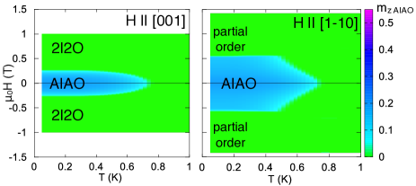
The phase diagrams have been calculated in Ref. 21 by Monte Carlo (MC) simulations applied to the XYZ Hamiltonian and using the coupling parameters available for the pure compound (See Figure 9 of this reference). These calculations were performed applying the field at high temperature and decreasing the temperature, thus corresponding to a FC procedure. Importantly, the so-called ordered parameter in these phase diagrams is associated to the AIAO component relative to the directions (defined as ) and not to the components that are actually measured.
We have performed mean-field (MF) calculations with the exchange parameters obtained for the pure compound [14]: rad (See Equation 1). Those calculations show that for the and field directions, the phase diagrams are identical whether focusing on the or -AIAO component (). This allows one to compare directly the calculated and measured phase diagrams. As previously obtained [29, 21], the calculated phase diagrams qualitatively reproduce the observations but the critical fields are smaller in the experiments (see Figures 8 and 11). In addition, the shape of the transition line for the direction is quite different from the measurements. The zero field transition temperature is overestimated, as expected for mean-field calculations.
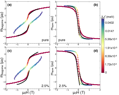
To clarify the differences between calculations and experiments, we have followed the “energy landscape” approach of Ref. 21. This consists in finding the configurations which minimize the classical energy, calculated numerically using the XYZ Hamiltonian (see Appendix D). Several solutions can be found, revealing local minima and thus metastable configurations. The corresponding moments are then plotted against the magnetic field, while a color scale is used to keep track of the value of the energy.
Figure 12(a-b) shows the results for the field applied along the direction together with the diffraction results in the pure sample. As expected from a simple symmetry analysis and the neutron results (discussed in Section IV.2), two magnetic configurations are equivalent in energy and define two branches for the evolution of magnetic moments vs field. This can be seen by plotting the magnetic component of the Nd3 moment (panel (a)), or the component (panel (b)). Two domains then probably form in the system when ramping the field, that cannot be distinguished in experiments. The field value at which the two branches merge, which corresponds to the suppression of the AIAO component, is slightly larger in the calculation than in the experiment, but roughly in the same range. The slight hysteresis observed experimentally may be due to a small field misalignment which would favor one domain over the other, resulting in metastable configurations, and reducing the critical field, in a similar way as for the direction that we will discuss below.
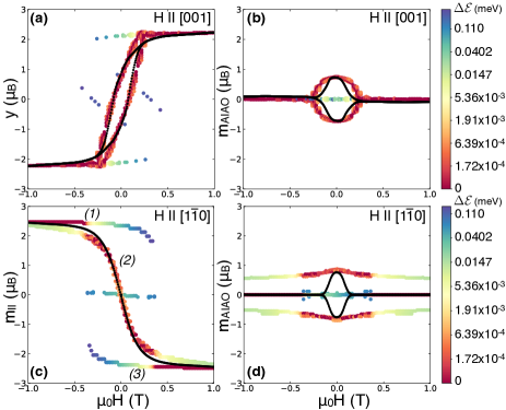
In the direction, the agreement between the calculations and the experiments is less convincing as can be seen in the panels (c-d) of Figure 12. The experimental (and thus the two domains) vanishes at much smaller field and more smoothly than in the calculations (panel (d)) where an abrupt jump is obtained. When focusing on the chains (Nd3 and Nd4), calculations for the parallel component (panel d) predict essentially three branches, labeled (1,2,3) on the figure: branches (1) and (2) correspond to an almost saturated moment, and are stable at high values of the (absolute) field. The central branch (3) is stable between about and 0.3 T. Looking at the color scale, and starting from T, the global energy minimum thus goes from a saturation branch to the other via the central branch. In this part, and the moment decreases smoothly. While in the calculations a little step is obtained when going from one branch to the other, concomitantly with the appearance and suppression of the “all in” or “all out” component, the experimental data seem to go continuously from one branch to the other.
A small jump is nevertheless observed in the derivative of the magnetization, but it is hysteretic and much weaker than in the present calculations. The discrepancy between the calculations and the experiments may lie in the subtlety of the situation: the two spins which remain disordered in the nearest neighbor classical approach may be sensitive to octupolar and long range dipolar couplings, or experience order by disorder effects [29, 32, 33]. It is clear from our results that these ingredients are not strong enough to affect the high field state since the Nd1 and Nd2 moments do not eventually order (which also excludes a strong misalignment of the field), but they may affect the low field picture.
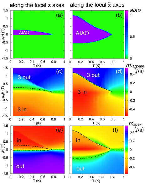
We now turn to the direction, where the description of the field induced process is less direct. Indeed, as already mentioned, the description in terms of an AIAO state is not relevant, due to the different fields felt by the apical and kagomé spins, the main consequence being that all the moments do not have the same “length” along the field direction. To get a clear insight of what happens in this case, it is convenient to define the parameter, which is equal to 1 if all the spins are “in” (or “out”) and 0 otherwise. This parameter can have a different value depending on whether it is defined with respect to the or to the directions, as illustrated in Figures 13 and 14 (a-b). Actually this is of great importance to understand the measured magnetic structure and phase diagrams.
At first, it appears simpler to discuss the phase diagram measured and calculated in field cooled conditions, since it is expected to describe the equilibrium state, and get rid of metastable states. Mean-field calculations shown in Figure 13 highlight two descriptions. The left column represents the parameter and magnetic components along , which can be directly related to the experiments. The right column shows the parameter and pseudo spin components along . Those are not observed in experiments, but we know from calculations that they are fully AIAO ordered in zero field. In the following, a distinction will be made between the configurations with respect to (-AIAO for instance) and to (denoted -AIAO).
Calculations show that the magnetic state is governed by the apical spins, as the kagomé spins simply follow the field direction (panels (c) and (d) of Figure 13). On the contrary, the apical pseudo spin is essentially along at low field, typically below T, hence forming tetrahedra either -“all in” or -“all out”. Above this threshold, the tetrahedra are -1I3O or -1O3I depending on the sign of the field. Interestingly, however, even if the pseudo spins are globally -AIAO, the actual magnetic configuration, i.e. with respect to , can be -1I3O (or -1O3I) (see Figure 15). When comparing quantitatively with the experimental data obtained from field cooled measurements (see Figure 10), the entrance in the gray region delimited by (maximum of the susceptibility) upon cooling seems to correspond to the entrance into a -AIAO state.
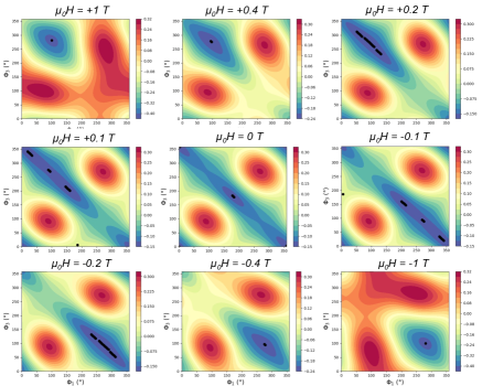
Similar calculations were performed by starting from a saturated state in negative field and increasing the field, similarly to the hysteresis loop / field sweeping experiments (see Figure 14). These calculations clearly reproduce the hysteretic behavior observed experimentally (see Figure 7). A transition is observed at T (right panels). It corresponds to the flipping of the kagomé spins from a -“in” to a -“out” configuration, and to a reduction of the ordered value for the apical spin. The change from the -AIAO to the -1I3O state, however, occurs gradually, the -AIAO component disappearing around T (left panels). These calculations thus cannot reproduce the transition measured at about T. To understand this discrepancy, which was not observed for the field cooled case, the method of the energy landscapes was used again (see Appendix D). As inferred from the experimental results, and previously discussed [21], this approach reveals the presence of two local energy minima, which result in metastable states when sweeping the field. Figure 16(a-b) shows the magnetic moment value associated to these local minima for the pure compound, while the color scale indicates the energy of the associated configuration. When comparing with mean-field calculations presented in Figure 14, these results reveal that the magnetic moment remain “trapped” on a single branch, which becomes metastable for positive fields. As previously noted in Ref. 21, the jump to the lowest energy branch, i.e. the critical field obtained in the mean-field approach corresponds to the point ( T) where the metastable branch disappears. The experimental magnetic moments obtained for the pure compound from the neutron diffraction data are displayed on top of these calculated points in Figure 16(a-b). Remarkably, the experimental points, especially for the kagomé moment, nearly fall on the calculated branches, suggesting that everything happens as if the system was jumping from the metastable branch to the minimum energy branch at a much smaller field (), following from there the absolute energy minimum. The magnetic configuration at this jump (for the red tetrahedra) changes from a -“all in” state to a -1I3O configuration. The system thus reaches its equilibrium state at a much smaller field than predicted in MF and MC calculations. The associated gain in energy obtained by jumping from one branch to another at is found to be about 50 mK. This shows the existence of relaxation processes not captured by calculations.
Experimentally, we have pointed out that (determined from curves) and (determined from ZFC-FC curves) define the same line in the phase diagram. Indeed, in a ZFC measurement, both domains are stabilized at low temperature. When applying a positive field (with our conventions) after ZFC, the “all out” domains of the red tetrahedra are on the equilibrium branch while the “all in” ones are on the metastable branch. When increasing the field and/or the temperature, the latter are suppressed. The system then reaches the equilibrium configuration, when the ZFC magnetization recovers the FC equilibrium one. This occurs at the same field / temperature point in the experimental phase diagram as the magnetization jump in the hysteresis. Incidentally, at low temperature, it roughly corresponds to the point where the -AIAO component disappears in the calculated field cooled phase diagram.
Finally, we can now understand the nature of the experimental phase diagram of Figure 10, when the field is applied along (the measurements being performed from a ZFC state, or a saturated state in a negative field): in the blue region both and components are AIAO (see the illustration in Figure 15(a)), and the system lies in a metastable state. In the gray one, only the component is AIAO, the one being 1I3O / 1O3I (see the illustration in Figure 15(b)), and the system has reached its ground state. The microscopic mechanism at the origin of the measured values of and separating these two regions nevertheless remains an issue.
V.2 Role of the Ti content
In this study, the phase diagrams have been established for three samples, the pure Nd2Zr2O7 compound and two Ti-substituted samples, NdZr1-xTiO7 with and 10 %. As shown in Table 2, the global pyrochlore stucture and its main properties (lattice parameter and oxygen position) are not significantly affected by the Ti substitution at low concentrations of Ti. Further structural studies are necessary to better characterize the disorder, but are beyond the scope of this article. From the present data, however, it is reasonable to consider that the titanium atoms are randomly distributed among the 16d sites of the crystallographic Fdm structure.
It is worth noting that the properties of the substituted polycrystalline samples are quantitatively different from the single crystal ones (smaller and slightly larger and ordered moments - see Appendix B). In the literature, larger and ordered moments were also reported in a pure single crystal compound [10]. The nature of the disorder and its consequences are thus not obvious, but nevertheless, two important features can be stressed. (i) The single ion properties of the neodymium ion are little affected by the presence of this disorder, the effective moment and local anisotropy being roughly similar in the three compounds. (ii) The presence of titanium is expected to mainly disturb the exchange paths, creating some distribution in the exchange parameters.
Indeed, the magnetic transition looks a bit broader in the AC susceptibility (see Figure 3) for substituted samples, but is still well defined. Strikingly, the AIAO ground state is characterized by a larger along with larger critical fields than in the pure sample, suggesting that the AIAO order is more robust. Since both characteristic parameters show a maximum at 2.5 % before decreasing at higher substitution concentration, the present study even suggests the existence of an optimum with respect to Ti-substitution level, where the stability of the ordered phase is best reinforced. In addition, the ordered magnetic moment is larger along the direction, thus corresponding to a lower angle, which indicates that the disorder tends to tilt the pseudo spins back towards the local axes. This picture is consistent with recent observations on Nd-based pyrochlores with a much stronger disorder on the -site [34, 35, 36], namely Nd2NbScO7 and Nd2GaSbO7. In the latter, it was nevertheless pointed out that the large obtained ordered moment and transition temperature are similar to the Nd2Sn2O7 compound [37]. It was thus proposed that the chemical pressure - which manifests in these two compounds by a small lattice parameter, compared to the zirconate counterpart - is a key ingredient to understand the magnetic properties, and which could be more decisive than the disorder itself.
Despite the absence of a microscopic description of the disorder which could help solving this issue, the phase diagram of the 2.5 % substituted sample can be further analyzed. To this end, we have computed the MF phase diagrams as well as the energy landscape using the exchange parameters determined by the magnetic excitations analysis [14] (see Figure 17(a,b)). The obtained values are rad (See Equation 1. For the sake of simplicity, was assumed for energy landscape calculations).
The first point that we stress is that, in mean-field calculations, the Néel temperature does not vary significantly between the results for the pure and 2.5 % substituted compounds. This is not surprising since the energy range of the parameters is similar in both, and the calculations strongly overestimate (while MC calculations underestimate it [21]). Nevertheless, experimentally, a strong variation of is observed between the three samples. This may be due to the competition at play between the Coulomb phase stabilized above the Néel temperature for the component and the -AIAO phase [21, 14] (see also Appendix A). This reminds the situation in Yb2Ti2O7 [17, 38, 39, 40], where the proximity of competing phases makes the transition temperature extremely sensitive to disorder. In Nd2Zr2O7, the disorder would promote the AIAO ordering at the expense of the Coulomb phase. This manifests in the exchange parameters by a smaller ratio in the substituted compound which is clearly in favor of the -AIAO phase.
When looking at the field induced behavior, calculations qualitatively reproduce the increase of the critical fields obtained experimentally in the and directions, as well as the nature of the field induced processes, which are similar to the pure compound. Nevertheless, there is no quantitative agreement in the obtained values for the critical field (see Table 3). When the field is applied along the direction, an increase of the critical field is obtained in the field cooled phase diagrams. Considering now the situation where the field is swept from saturation, almost no difference is obtained in the calculated critical field (of about 1.2 T) corresponding to the jump from a metastable domain to the equilibrium. When looking in more details at the branches displayed in Figure 16(c,d), we can see that their shape is quite different from the pure compound case, even if the two branches merge at almost the same field of about 1.2 T. The data obtained from the neutron field sweeping analysis falls again on the branches, even if the agreement is less good for the kagomé moment in high field. The jump from one branch to the other occurs experimentally at T, which corresponds to an energy difference of 50 mK, comparable to the case of the pure compound.
From our experimental and calculation results, the samples comparison thus shows that despite quite strong quantitative differences on the Néel temperature or on the ordered moment, the field induced behaviors remain similar, the critical fields being shifted to larger values in the substituted samples. The level of disorder introduced in the present study on the non magnetic site is not strong enough to destabilize the -AIAO ordering, and on the contrary seems to reinforce it. As previously mentioned, recent studies show that the AIAO state resists to an even stronger disorder [34, 35, 36]. Consequently, it may be relevant to directly make a substitution on the magnetic site in order to test the stability of the AIAO state on dilution, and to possibly reach the predicted quantum spin liquid ground state when the ratio decreases [12, 41].
VI Conclusion
In this work, phase diagrams for fields applied along the three main high symmetry crystallographic directions have been constructed for three sample compositions of the Nd2(Zr1-xTix)2O7 family. A systematic analysis of neutron diffraction data was employed, combined with low temperature magnetization measurements. Depending on the field direction, different phases are obtained, either AIAO, 2I2O or 1I3O / 1O3I. The present work essentially establishes the stability regions of the AIAO phase, and shows that a small amount of disorder further reinforces this phase, both in field and temperature. In addition, the comparison with calculations performed using the XYZ Hamiltonian shows how the field induced phases (2I2O and 1I3O / 1O3I) are connected to the two and domains, and elucidates the apparent strong discrepancy between calculated and measured critical fields when the field is applied along the direction. Further work on the microscopic mechanisms at play in the domain selection are nevertheless needed to quantitatively understand the critical field values.
Acknowledgements.
The work at the University of Warwick was supported by EPSRC, UK through Grant EP/T005963/1. M.L. and S.P. acknowledge financial support from the French Federation of Neutron Scattering (2FDN) and Université Grenoble-Alpes (UGA). F.D, E.L. and S.P. acknowledge financial support from ANR, France, Grant No. ANR-19-CE30-0040-02.| Powder Samples | Ti concentration | O2 position | Lattice parameter | Ordered moment | |||
|---|---|---|---|---|---|---|---|
| [%] | [Å] | [mK] | [mK] | [] | [] | ||
| 0 | 0.3366 | 10.69 | 370 | 225 | 2.42 | ||
| 2.8 | 0.3360 | 10.67 | 420 | 70 | 2.53 | ||
| 11.2 | 0.3359 | 10.64 | 430 | 80 | 2.51 |
Appendix A Notes about fragmentation
Prior experimental investigations of Nd2Zr2O7 [9, 11], have pointed to the fact that the ground state of this material bears similarities with the fragmentation phenomenon exposed in Ref. 42. In particular, the fact that only 1/3 of the total moment is ordered was one of the strongest arguments.
In this theory, the proliferation of spin flips out of the spin ice 2I2O manifold, i.e. 1O3I and 1I3O local configurations, or monopoles in the field language, produces a “charged” state, described by two fragments that identify with the Helmholtz-Hodge decomposition of the spin ice emergent magnetic field :
where is a scalar potential, and the vector potential. In this decomposition, the first term is divergence-full and carries the total gauge charge , . The second term encodes the position of the spin flip and is divergence-less (). In the case of spin ice, the ground state is naturally the vacuum of charges (). However, a different ground state appears if a non-zero density of monopoles becomes favored for energetic and/or entropic reasons. Provided the fluid of monopoles crystallizes and forms a staggered pattern, the new ground state is fragmented, comprised of an AIAO component carried by the divergence full term on top of a secondary Coulomb phase carried by the divergence free term. Importantly, the charge per tetrahedron () is only half the charge carried by a standard AIAO state (). As a result, in a neutron diffraction experiment, the fragmented state is characterized by an AIAO ordering with an ordered magnetic moment reduced by a factor of two, on top of a spin ice pattern described by .
The XYZ Hamiltonian approach is quite far away from this theory of fragmentation. Its phase diagram was studied using the gauge mean field theory (gMFT) in Ref. 18, 43. It presents unconventional quantum spin liquid states [44, 45, 46, 47, 48, 49, 50], but also includes classical states. These are ordered AIAO-like phases, with pseudo spins pointing along the direction. At the mean field level, they are stabilized provided with . In Ref. 18, those states are labeled AIAO and AFO (the latter corresponding to an antiferro-octupolar state). Interestingly, the experimental couplings place Nd2Zr2O7 close to the border between the liquid phase and the -AIAO state in the gMFT phase diagram determined by Huang et al. [18]. The most recent experiments actually support a picture where the paramagnetic regime above the AIAO Néel temperature in Nd2Zr2O7 is indeed such a coulombic phase [13, 14], stabilized both by the strong positive as well as entropic effects.
Ref. 12 describes a mean field theory of this XYZ model. For the Nd2Zr2O7 parameters, the ground state is an AIAO magnetic configuration of the pseudo spins pointing along the axes and is thus a fully charged state. However, it turns out that the dynamical magnetization can still be “Helmholtz-Hodge” decomposed in terms of (lattice) divergence-free and divergence-full fields [12]. On the one hand, the flat spin ice mode identifies with the divergence-free dynamical field. Its pinch point pattern relates it to the divergence free condition . It is formed by individual precessions around the local magnetization of spins belonging to closed loops in the pyrochlore lattice. On the other hand, the dispersing branch corresponds to the divergence-full dynamical field and is the signature of charge propagation throughout the diamond lattice. This branch is characterized by a beautiful half moon pattern when moving away from the pinch points. Such a pattern is typical of a curl free condition, which characterizes the charges, since [51].
Appendix B Powder samples
Aiming at a first description of the physical properties of the substituted samples, magnetic measurements along with neutron diffraction were performed on the substituted powder samples. The very low temperature magnetization and susceptibility were measured in the same magnetometer developed at the Institut Néel as single crystals. For these measurements, the powder samples were packed in a copper pouch with apiezon grease to ensure proper thermalization. Structural parameters were obtained with the high resolution powder neutron D2B (ILL) diffractometer using Å. The ground state magnetic structure in zero applied field was determined on the powder neutron G4.1 (LLB-Orphée, France) diffractometer using Å. A dedicated vanadium sample holder was used, loaded with 4He pressure of about bars to ensure thermalization. Structural and magnetic parameters were refined with the Fullprof suite [26].
The structural data could be refined with a pyrochlore structure (Fdm space group). Magnetic properties are qualitatively similar to the pure compound properties (see Table 4): from Curie-Weiss fits between and K, the low temperature effective moment is estimated to and a small (70 - 80 mK) but positive Curie-Weiss temperature could be extracted, indicative of effective ferromagnetic interactions. An antiferromagnetic transition is found to occur above 400 mK for both compounds in the susceptibility, but which is sharper in the 2.5 %-substituted sample. Neutron diffraction refinements could show that the magnetic structure is AIAO, like in the pure compound, with an ordered moment of about at low temperature (See Figure 18).
Appendix C Analysis of the field sweeping measurements
| 0 | [001] | (2,2,0), (0,4,0), (1,1,1), (2,0,0), (3,1,-1) |
| [1-10] | (0,0,2), (0,0,4), (1,1,3), (2,2,0), (3,3,1), (1,1,1) | |
| [111] | (2,0,0), (2,-2,0), (1,-1,1), (1,3,-1) | |
| 2.5 % | [001] | (2,-2,0), (0,4,0), (-1,-1,-1), (-1,1,-1), (-3,1,-1), (-1,-3,-1), (-3,-3,-1) |
| [1-10] | (0,0,2), (0,0,4), (1,1,3), (2,2,0), (3,3,1), (3,3,-1) | |
| [111] | (-2,0,0), (-2,2,0), (-1,1,-1), (-1,-3,1) | |
| 10 % | [001] | (2,-2,0), (0,4,0), (1,-1,1), (2,0,0), (3,1,1), (-3,3,1) |
| [111] | (-2,0,0), (-2,2,0), (-1,1,-1), (-1,-3,1) |
To complete the diffraction measurements, the intensity of selected Bragg peaks was recorded while ramping the field back and forth from T to T ( T/min was the minimum sweeping speed) to obtain a “continuous” evolution vs field. The analysis of those field sweeping measurements relies on the comparison between the experimental magnetic intensities and the calculated ones , given the various models described in the main text and the usual definitions of the neutron intensities:
and denote the magnetic moment and position of the spin in the unit cell. The method that was developed in this work involves the minimization of a defined as:
| (6) |
is the set of parameters to be refined. The index runs over a list of vectors given in Table 5 and which were chosen carefully as they show a significant evolution vs field. is the experimental intensity. is derived from the calculated intensity but is defined using the moments and determined with Fullprof at two reference fields and T:
This definition ensures that
and
so that and minimize at and respectively. This definition thus puts severe constraints on the minimization.
A home made program was then used to calculate over a grid for the parameters , and to keep the values which minimize it. As different combinations of parameters can give a consistent result, a weight is associated to each solution and takes the form of a color scale in the figures presented in the main text: from blue, the worst , to red, the best . It is worth mentioning that this analysis cannot distinguish positive and negative values of the magnetic moments. A new criterion was thus added to keep only the values giving a positive product of the magnetization times the applied field (this is justified since no remanent magnetization has been observed in the magnetization curves). The points obtained with FullProf from the data collections at fixed fields eventually confirm the consistency of the analysis.
Appendix D Energy landscapes
Following Ref. [21], it is instructive to calculate the energy landscape in the presence of a magnetic field to better understand the origin of the hysteresis. Writing the four spins in a tetrahedron in their local frame as:
| (7) |
the classical exchange and Zeeman energy per tetrahedron can be evaluated using the Hamiltonian given by Eq. 1 and Eq. 2 (and neglecting the octupolar exchange term). The numerical values K, 1.18 K, rad and K, K, rad were used, corresponding to the pure and the 2.5 % substituted sample parameters respectively.
D.1 Field along
In the particular case of , the angles are identical within the two subgroups (1,2) and (3,4), hence:
At large positive field, the minimum of the energy is obtained for , i.e. which corresponds to the moments of the (3,4) atoms parallel to their axes and the (1,2) ones anti-parallel to their axes. At zero field, two minima occur, corresponding to or , i.e. to the domains and of the ordered state. Figure 19 illustrates this evolution. It displays several contour plots of as a function of and for the case. The black dots show the position of the minima. Upon increasing field, two minima appear, separate to give rise to the and domains, and finally reconnect at a higher field. With a sufficiently large field, a single solution survives.
D.2 Field along
For , the angles are identical for the kagomé spins and we are left with two variables (kagomé) and (apical). The classical energy writes:
At large positive field, the minimum of the energy is obtained for , i.e. which corresponds to spins 1, 3, 4 parallel to their axes and spin 2 anti-parallel to its axis. At zero field, two minima occur, corresponding to or , i.e. to the two domains of the AIAO configuration.
D.3 Field along
For , two different regimes can be considered. At large fields, , and , hence the classical energy:
At large positive field, the minimum of the energy is obtained for , i.e. which corresponds to spin 3 antiparallel to its axis and spin 4 parallel to its axis.
At small fields, , no simplification appears but and we are left with three independent variables . The classical energy writes:
The minimization of in the general case should be carried out in the three-dimensional space spanned by the three angles.
References
- Lacroix et al. [2011] C. Lacroix, P. Mendels, and F. Mila, eds., Introduction to Frustrated Magnetism (Springer-Verlag, Berlin, 2011).
- Gingras and McClarty [2014] M. J. P. Gingras and P. A. McClarty, Quantum spin ice: a search for gapless quantum spin liquids in pyrochlore magnets, Rep. Prog. Phys. 77, 056501 (2014).
- Gardner et al. [2010] J. S. Gardner, M. J. P. Gingras, and J. E. Greedan, Magnetic pyrochlore oxides, Rev. Mod. Phys. 82, 53 (2010).
- Harris et al. [1997] M. J. Harris, S. T. Bramwell, D. F. McMorrow, T. Zeiske, and K. W. Godfrey, Geometrical frustration in the ferromagnetic pyrochlore Ho2Ti2O7, Phys. Rev. Lett. 79, 2554 (1997).
- Ramirez et al. [1999] A. P. Ramirez, A. Hayashi, R. J. Cava, R. Siddharthan, and B. S. Shastry, Zero-point entropy in ‘spin ice’, Nature 399, 333 (1999).
- Henley [2005] C. L. Henley, Power-law spin correlations in pyrochlore antiferromagnets, Phys. Rev. B 71, 014424 (2005).
- Isakov et al. [2004] S. V. Isakov, K. Gregor, R. Moessner, and S. L. Sondhi, Dipolar spin correlations in classical pyrochlore magnets, Phys. Rev. Lett. 93, 167204 (2004).
- Fennell et al. [2009] T. Fennell, P. P. Deen, A. R. Wildes, K. Schmalzl, D. Prabhakaran, A. T. Boothroyd, R. J. Aldus, D. F. McMorrow, and S. T. Bramwell, Magnetic coulomb phase in the spin ice Ho2Ti2O7, Science 326, 415 (2009).
- Lhotel et al. [2015] E. Lhotel, S. Petit, S. Guitteny, O. Florea, M. Ciomaga Hatnean, C. Colin, E. Ressouche, M. R. Lees, and G. Balakrishnan, Fluctuations and all-in–all-out ordering in dipole-octupole Nd2Zr2O7, Phys. Rev. Lett. 115, 197202 (2015).
- Xu et al. [2015] J. Xu, V. K. Anand, A. K. Bera, M. Frontzek, D. L. Abernathy, N. Casati, K. Siemensmeyer, and B. Lake, Magnetic structure and crystal field states of the pyrochlore antiferromagnet Nd2Zr2O7, Phys. Rev. B 92, 224430 (2015).
- Petit et al. [2016] S. Petit, E. Lhotel, B. Canals, M. Ciomaga Hatnean, J. Ollivier, H. Mutka, E. Ressouche, A. R. Wildes, M. R. Lees, and G. Balakrishnan, Observation of magnetic fragmentation in spin ice, Nat. Phys. 12, 746 (2016).
- Benton [2016] O. Benton, Quantum origins of moment fragmentation in Nd2Zr2O7, Phys. Rev. B 94, 104430 (2016).
- Xu et al. [2020] J. Xu, O. Benton, A. T. M. N. Islam, T. Guidi, G. Ehlers, and B. Lake, Order out of a coulomb phase and higgs transition: Frustrated transverse interactions in Nd2Zr2O7, Phys. Rev. Lett. 124, 097203 (2020).
- Léger et al. [2020] M. Léger, E. Lhotel, M. Ciomaga Hatnean, J. Ollivier, A. R. Wildes, S. Raymond, E. Ressouche, G. Balakrishnan, and S. Petit, Spin dynamics and unconventional coulomb phase in Nd2Zr2O7 (2020), arXiv:2101.09049.
- Taniguchi et al. [2013] T. Taniguchi, H. Kadowaki, H. Takatsu, B. Fåk, J. Ollivier, T. Yamazaki, T. J. Sato, H. Yoshizawa, Y. Shimura, T. Sakakibara, T. Hong, K. Goto, L. R. Yaraskavitch, and J. B. Kycia, Long-range order and spin-liquid states of polycrystalline Tb2+xTi2-xO7+y, Phys. Rev. B 87, 060408(R) (2013).
- Shirai et al. [2017] M. Shirai, R. S. Freitas, J. Lago, S. T. Bramwell, C. Ritter, and I. Živković, Doping-induced quantum crossover in Er2Ti2-xSnxO7, Phys. Rev. B 96, 180411(R) (2017).
- Arpino et al. [2017] K. E. Arpino, B. A. Trump, A. O. Scheie, T. M. McQueen, and S. M. Koohpayeh, Impact of stoichiometry of Yb2Ti2O7 on its physical properties, Phys. Rev. B 95, 094407 (2017).
- Huang et al. [2014] Y.-P. Huang, G. Chen, and M. Hermele, Quantum spin ices and topological phases from dipolar-octupolar doublets on the pyrochlore lattice, Phys. Rev. Lett. 112, 167203 (2014).
- Opherden et al. [2017] L. Opherden, J. Hornung, T. Herrmannsdörfer, J. Xu, A. T. M. N. Islam, B. Lake, and J. Wosnitza, Evolution of antiferromagnet domains in the all-in/all-out ordered pyrochlore Nd2Zr2O7, Phys. Rev. B 95, 184418 (2017).
- Note [1] A weak contribution to the neutron scattering cross section is expected at large wavevectors.
- Xu et al. [2019] J. Xu, O. Benton, V. K. Anand, A. T. M. N. Islam, T. Guidi, G. Ehlers, E. Feng, Y. Su, A. Sakai, P. Gegenwart, and B. Lake, Anisotropic exchange hamiltonian, magnetic phase diagram and domain inversion of Nd2Zr2O7, Phys. Rev. B 99, 144420 (2019).
- Ciomaga Hatnean et al. [2015] M. Ciomaga Hatnean, M. R. Lees, and G. Balakrishnan, Growth of single-crystals of rare-earth zirconate pyrochlores, Zr2O7 (with La, Nd, Sm, and Gd) by the floating zone technique, J. Cryst. Growth 418, 1 (2015).
- Ciomaga Hatnean et al. [2016] M. Ciomaga Hatnean, C. Decorse, M. R. Lees, O. A. Petrenko, and G. Balakrishnan, Zirconate pyrochlore frustrated magnets: Crystal growth by the floating zone technique, Crystals 6, 79 (2016).
- Paulsen [2001] C. Paulsen, Introduction to physical techniques in molecular magnetism: Structural and macroscopic techniques (Servicio de Publicaciones de la Universidad de Zaragoza, 2001) Chap. DC magnetic measurements, p. 1.
- Aharoni [1998] A. Aharoni, Demagnetizing factors for rectangular ferromagnetic prisms, J. App. Phys. 83, 3432 (1998).
- Rodriguez-Carvajal [1993] J. Rodriguez-Carvajal, Recent advances in magnetic structure determination by neutron powder diffraction, Physica B 192, 55 (1993).
- Harris et al. [1998] M. J. Harris, S. T. Bramwell, P. C. W. Holdsworth, and J. D. M. Champion, Liquid-gas critical behavior in a frustrated pyrochlore ferromagnet, Phys. Rev. Lett. 81, 4496 (1998).
- Note [2] It is worth mentioning that in a trial experiment where the field was not perfectly aligned along (about 4 degrees while less than 1 in the present experiment), such a non-zero moment could be refined, suggesting that it is likely a by product of the ill-aligned component of the field.
- Xu et al. [2018] J. Xu, A. T. M. N. Islam, I. N. Glavatskyy, M. Reehuis, J. U. Hoffmann, and B. Lake, Field induced quantum spin 1/2 chains and disorder in Nd2Zr2O7, Phys. Rev. B 98, 060408(R) (2018).
- Lhotel et al. [2018] E. Lhotel, S. Petit, M. Ciomaga Hatnean, J. Ollivier, H. Mutka, E. Ressouche, M. R. Lees, and G. Balakrishnan, Evidence for dynamic kagome ice, Nat. Commun. 9, 3786 (2018).
- Opherden et al. [2018] L. Opherden, T. Bilitewski, J. Hornung, T. Herrmannsdörfer, A. Samartzis, A. T. M. N. Islam, V. K. Anand, B. Lake, R. Moessner, and J. Wosnitza, Inverted hysteresis and negative remanence in a homogeneous antiferromagnet, Phys. Rev. B 98, 180403(R) (2018).
- Guruciaga et al. [2016] P. C. Guruciaga, M. Tarzia, M. V. Ferreyra, L. F. Cugliandolo, S. A. Grigera, and R. A. Borzi, Field-tuned order by disorder in frustrated Ising magnets with antiferromagnetic interactions, Phys. Rev. Lett. 117, 167203 (2016).
- Placke et al. [2020] B. Placke, R. Moessner, and O. Benton, Hierarchy of energy scales and field-tunable order by disorder in dipolar-octupolar pyrochlores, Phys. Rev. B 102, 245102 (2020).
- [34] C. Mauws, N. Hiebert, M. Rutherford, H. D. Zhou, Q. Huang, M. B. Stone, N. P. Butch, Y. Su, E. S. Choi, and Z. Y. andChristopher R. Wiebe, Order by chemical disorder: Destruction of moment fragmentation by charge disorder in Nd2ScNbO7, arXiv:1906.10703.
- [35] A. Scheie, M. Sanders, Y. Qiu, T. Prisk, R. Cava, and C. Broholm, Beyond magnons in Nd2ScNbO7: An ising pyrochlore antiferromagnet with all in all out order and random fields, arXiv:2102.13656.
- [36] S. J. Gomez, P. M. Sarte, M. Zelensky, A. M. Hallas, B. A. Gonzalez, K. H. Hong, E. J. Pace, S. Calder, M. B. Stone, Y. Su, E. Feng, M. D. Le, C. Stock, J. P. Attfield, S. D. Wilson, C. R. Wiebe, and A. A. Aczel, Absence of moment fragmentation in the mixed -site pyrochlore Nd2GaSbO7, arXiv:2104.00791.
- Bertin et al. [2015] A. Bertin, P. Dalmas de Réotier, B. Fåk, C. Marin, A. Yaouanc, A. Forget, D. Sheptyakov, B. Frick, C. Ritter, A. Amato, C. Baines, and P. J. C. King, Nd2Sn2O7: An all-in—all-out pyrochlore magnet with no divergence-free field and anomalously slow paramagnetic spin dynamics, Phys. Rev. B 92, 144423 (2015).
- Robert et al. [2015] J. Robert, E. Lhotel, G. Remenyi, S. Sahling, I. Mirebeau, C. Decorse, B. Canals, and S. Petit, Spin dynamics in the presence of competing ferromagnetic and antiferromagnetic correlations in Yb2Ti2O7, Phys. Rev. B 92, 064425 (2015).
- Jaubert et al. [2015] L. D. C. Jaubert, O. Benton, J. G. Rau, J. Oitmaa, R. R. P. Singh, N. Shannon, , and M. J. P. Gingras, Are multiphase competition and order by disorder the keys to understanding Yb2Ti2O7 ?, Phys. Rev. Lett. 115, 267208 (2015).
- Scheie et al. [2020] A. Scheie, J. Kindervater, S. Zhang, H. J. Changlani, G. Sala, G. Ehlers, A. Heinemann, G. S. Tucker, S. M. Koohpayeh, and C. Broholm, Multiphase magnetism in Yb2Ti2O7, PNAS 117, 27245 (2020).
- Benton [2020] O. Benton, Ground-state phase diagram of dipolar-octupolar pyrochlores, Phys. Rev. B 102, 104408 (2020).
- Brooks-Bartlett et al. [2014] M. E. Brooks-Bartlett, S. T. Banks, L. D. C. Jaubert, A. Harman-Clarke, and P. C. W. Holdsworth, Magnetic moment fragmentation and monopole crystallization, Phys. Rev. X 4, 011007 (2014).
- Li and Chen [2017] Y.-D. Li and G. Chen, Symmetry enriched topological orders for dipole-octupole doublets on a pyrochlore lattice, Phys. Rev. B 95, 041106(R) (2017).
- Hermele et al. [2004] M. Hermele, M. P. A. Fisher, and L. Balents, Pyrochlore photons: The spin liquid in a three-dimensional frustrated magnet, Phys. Rev. B 69, 064404 (2004).
- Shannon et al. [2012] N. Shannon, O. Sikora, F. Pollmann, K. Penc, and P. Fulde, Quantum ice: A quantum monte carlo study, Phys. Rev. Lett. 108, 067204 (2012).
- Benton et al. [2012] O. Benton, O. Sikora, and N. Shannon, Seeing the light: Experimental signatures of emergent electromagnetism in a quantum spin ice, Phys. Rev. B 86, 075154 (2012).
- Savary and Balents [2012] L. Savary and L. Balents, Coulombic quantum liquids in spin-1/2 pyrochlores, Phys. Rev. Lett. 108, 037202 (2012).
- Savary and Balents [2013] L. Savary and L. Balents, Spin liquid regimes at nonzero temperature in quantum spin ice, Phys. Rev. B 87, 205130 (2013).
- Hao et al. [2014] Z. Hao, A. G. R. Day, and M. J. P. Gingras, Bosonic many-body theory of quantum spin ice, Phys. Rev. B 90, 214430 (2014).
- Huang et al. [2018] C.-J. Huang, Y. Deng, Y. Wan, and Z. Y. Meng, Dynamics of topological excitations in a model quantum spin ice, Phys. Rev. Lett. 120, 167202 (2018).
- Yan et al. [2018] H. Yan, R. Pohle, and N. Shannon, Half moons are pinch points with dispersion, Phys. Rev. B 98, 140402(R) (2018).