Essentiality of the Non-stoquastic Hamiltonians and Driver Graph Design in Quantum Optimization Annealing

Abstract

One of the distinct features of quantum mechanics is that the probability amplitude can have both positive and negative signs, which has no classical counterpart as the classical probability must be positive. Consequently, one possible way to achieve quantum speedup is to explicitly harness this feature. Unlike a stoquastic Hamiltonian whose ground state has only positive amplitudes (with respect to the computational basis), a non-stoquastic Hamiltonian can be eventually stoquastic or properly non-stoquastic when its ground state has both positive and negative amplitudes. In this paper, we describe that, for some hard instances which are characterized by the presence of an anti-crossing (AC) in a transverse-field quantum annealing (QA) algorithm, how to design an appropriate XX-driver graph (without knowing the prior problem structure) with an appropriate XX-coupler strength such that the resulting non-stoquastic QA algorithm is proper-non-stoquastic with two bridged anti-crossings (a double-AC) where the spectral gap between the first and second level is large enough such that the system can be operated diabatically in polynomial time. The speedup is exponential in the original AC-distance, which can be sub-exponential or exponential in the system size, over the stoquastic QA algorithm, and possibly the same order of speedup over the state-of-the-art classical algorithms in optimization. This work is developed based on the novel characterizations of a modified and generalized parametrization definition of an anti-crossing in the context of quantum optimization annealing introduced in [4].

1 Introduction

Adiabatic quantum computation in the quantum annealing form is a quantum computation model proposed for solving the NP-hard combinatorial optimization problems, see [1] for the history survey and references therein. A quantum annealing algorithm is described by a system Hamiltonian

$${\mathcal{H}}(s)=(1-s){\mathcal{H}}_{\mathsf{driver}}+s{\mathcal{H}}_{\mathsf{problem}}$$ (1)

where the driver Hamiltonian ${\mathcal{H}}_{\mathsf{driver}}$, whose ground state is known and easy to prepare; the problem Hamiltonian ${\mathcal{H}}_{\mathsf{problem}}$, whose ground state encodes the solution to the optimization problem; $s\in[0,1]$ is a parameter that depends on time. A typical example of the system Hamiltonian is the transverse-field Ising model (TFIM) where the driver Hamiltonian is ${\mathcal{H}}_{X}=-\sum_{i\in{\mathsf{V}}(G)}\sigma^{x}_{i}$, and the problem Hamiltonian ${\mathcal{H}}_{\mathsf{problem}}$ is an Ising Hamiltonian: ${\mathcal{H}}_{\mathsf{Ising}}=\sum_{i\in{\mathsf{V}}(G)}h_{i}\sigma^{z}_{i}+\sum_{ij\in{\mathsf{E}}(G)}J_{ij}\sigma^{z}_{i}\sigma^{z}_{j}$ defined on a problem graph $G=({\mathsf{V}}(G),{\mathsf{E}}(G))$, which encodes the optimization problem to be solved. The quantum processor that implements the many-body system Hamiltonian is also referred to as a quantum annealer (QA). The QA system is initially prepared in the known ground state of ${\mathcal{H}}_{\mathsf{driver}}$, and then through a quantum evolution process, it reaches the ground state of ${\mathcal{H}}_{\mathsf{problem}}$ at the end of the evolution. We will consider the driver Hamiltonian ${\mathcal{H}}_{\mathsf{driver}}$ that includes both X-driver term: ${\mathcal{H}}_{X}=-\sum_{i\in{\mathsf{V}}(G)}\sigma^{x}_{i}$, and XX-driver term ${\mathcal{H}}_{{\mathsf{XX}}}=J_{\mathsf{xx}}\sum_{ij\in{\mathsf{E}}(G_{\mathsf{driver}})}\sigma_{i}^{x}\sigma_{j}^{x}$ where $G_{\mathsf{driver}}$ is the driver graph, and $J_{\mathsf{xx}}$ can be a positive or negative real number. A Hamiltonian is originally defined to be stoquastic [2] if its non-zero off-diagonal matrix elements in the computational basis are all negative; otherwise, it is called non-stoquastic. Thus, ${\mathcal{H}}_{{\mathsf{XX}}}$ is stoquastic if $J_{\mathsf{xx}}<0$ and non-stoquastic if $J_{\mathsf{xx}}>0$. Below, we will discuss a refinement of the non-stoquasticity. We consider the following three types of driver Hamiltonians:

$${\mathcal{H}}_{\mathsf{driver}}=\left\{\begin{array}[h]{ll}{\mathcal{H}}_{X}&(D1)\\ {\mathcal{H}}_{X}+{\mathcal{H}}_{{\mathsf{XX}}}&(D2)\\ {\mathcal{H}}_{X}+s{\mathcal{H}}_{{\mathsf{XX}}}&(D3)\end{array}\right.$$

Type $(D1)$ is the standard transverse field driver Hamiltonian with the uniform superposition state as the (initial) ground state. At this point it is unclear what kind of $(D2)$ Hamiltonian is possible to prepare experimentally, even if the (initial) ground state is known. For this reason, we consider the type $(D3)$ driver Hamiltonian, which is known as the catalyst [3], with the uniform superposition state as the (initial) ground state. In this paper, we consider the NP-hard MWIS problem (which any Ising problem can be easily reduced to [4]). We will denote the system Hamiltonian in Eq. (1) for solving the MWIS problem on the weighted $G$ by ${\mathcal{H}}^{\mathsf{TFIM}}(G)$ when ${\mathcal{H}}_{\mathsf{driver}}={\mathcal{H}}_{X}$; and by ${\mathcal{H}}^{\mathsf{XX\!-\!Sys}}(J_{\mathsf{xx}},G_{\mathsf{driver}},G)$ when ${\mathcal{H}}_{\mathsf{driver}}={\mathcal{H}}_{X}+s{\mathcal{H}}_{{\mathsf{XX}}}={\mathcal{H}}_{X}+s(J_{\mathsf{xx}}\sum_{ij\in{\mathsf{E}}(G_{\mathsf{driver}})}\sigma_{i}^{x}\sigma_{j}^{x})$, without explicitly stating the weight function $w$ on $G$, and omitting the time parameter $(s)$, $s\in[0,1]$.

Typically, QA is assumed to be operated adiabatically, and the system remains in its instantaneous ground state throughout the entire evolution process. However, QA can be operated non-adiabatically when the system undergoes diabatic transitions to the excited states and then return to the ground state. The former is referred to as AQA, and the latter as DQA. Recently, some quantum enhancement with DQA were discussed in [5]. It is worthwhile to point out that the DQA defined there means that the system remains in a subspace spanned by a band of eigenstates of the system Hamiltonian and it does not necessarily return to the ground state at the end of the evolution. We are interested in successfully solving the optimization problem and therefore require the system returns to the ground state. To distinguish these two versions, we shall refer to our version of DQA as DQA-GS. DQA-GS has been exploited for the possible quantum speedup by an oracular stoquastic QA algorithm in[6, 7]. More discussion on this in Section 3.

The running time of a QA algorithm is the total evolution time, $t_{f}=s^{-1}(1)$. According to the Adiabatic Theorem (see, e.g.,[9] for a rigorous statement), the run time of an AQA algorithm is inversely proportional to a low power of the minimum spectral gap (min-gap), $\Delta_{10}(s^{*})=\min_{s}E_{1}(s)-E_{0}(s)$, where $E_{0}(s)$ ($E_{1}(s)$, resp.) is the energy value of the ground state (the first excited state, resp. ) of ${\mathcal{H}}(s)$. Thus far, the possible quantum speedup of the transverse-field Ising-based QA (TFQA) as a heuristic solver for optimization problem over state-of-the-art classical (heuristic) algorithms has been called into questions, see [5] for a discussion. As a matter of fact, the min-gap can be exponentially small in the problem size and thus a TFQA algorithm can take an exponential time, without achieving a quantum advantage. Indeed, one can easily construct instances that have an exponentially small gap due to an anti-crossing between levels corresponding to local and global minima of the optimization function, see e.g., [4, 10, 11].

Anti-crossing (AC), also known as avoided level crossing or level repulsion, is a well-known concept for physicists. In the context of adiabatic quantum optimization (AQO), the small-gap due to an anti-crossing has been explained in terms of some established physics theory, such as first-order phase transition [10], Anderson localization [12]. In these two cases, the argument was based on applying the perturbation theory at the end of evolution where the anti-crossing occurs. Such an anti-crossing was later referred to as a perturbative crossing, see e.g. [3]. A parametrization definition of an anti-crossing was first introduced by Wilkinson in [14], and was used in [15] to study the effect of noise on the QA system. In [4], we gave a parametrization definition for an anti-crossing in the context of quantum optimization annealing where we also describe the behavior of the energy states that are involved in the anti-crossing, including the symmetry-and-anti-symmetry (SAS) property of the two states at the anti-crossing point.

In this paper, we modify and generalize the parametrization definition of the anti-crossing in [4]. We derive some novel characteristics of such an anti-crossing and develop it into an analytical tool for the design and analysis of the QA algorithm. In particular, (1) we discover the significance of the sign of the coefficients of the states involved in the anti-crossing which leads to the revelation of the significant distinction between the proper-non-stoquastic and eventually-stoquastic Hamiltonians (to be elaborated below). (2) We derive the necessary conditions for the formation of an anti-crossing. This provides us algorithmic insight into the relationship between an anti-crossing and the structure of the local and global minima of the problem. (3) We derive two different formulae for computing the AC-gap. One is descriptive in that we can use it to study how the AC-gap changes (without actually computing the gap size) as we vary one parameter in the system Hamiltonian, including either the parameters in the problem Hamiltonian or the $\mathsf{XX}$-coupler strength in the driver Hamiltonian. The other gives AC-gap bound asymptotically in terms of AC-distance. The gap size is not only important for the run-time of the adiabatic algorithm, but it is also crucial for the analysis of the diabatic transition in DQA setting.

We now describe our algorithm, named Dic-Dac-Doa, which stands for: Driver graph from Independent-Cliques; Double Anti-Crossing; Diababtic quantum Optimization Annealing. The idea is to design an appropriate $\mathsf{XX}$-driver graph $G_{\mathsf{driver}}$ with an appropriate $\mathsf{XX}$-coupler strength $J_{\mathsf{xx}}$ such that for an instance $G$ (which is characterized by the presence of an AC in the TFQA algorithm described by ${\mathcal{H}}^{\mathsf{TFIM}}(G)$), the corresponding non-stoquastic Hamiltonian system that is described by ${\mathcal{H}}^{\mathsf{XX\!-\!Sys}}(J_{\mathsf{xx}},G_{\mathsf{driver}},G)$ has a double-AC or a sequence of nested double-ACs, or a double multi-level anti-crossing, with the desired property, such that one can apply DQA-GS successfully to solve the optimization problem in polynomial time. A high-level description of Dic-Dac-Doa is described in Table 1. The input to the algorithm is a vertex-weighted graph $G$ of the MWIS problem with the assumption that it has a special independent-cliques (IC) structure. We refer to such an instance as a GIC (graph of independent cliques) instance. Each clique in the IC is a clique of partites, with each partite consisting of either one single vertex or an independent set (of vertices). When all partites are single vertices, the clique of partites is the normal clique; otherwise the clique is also known as the multi-partite graph (not necessarily complete). The size of the clique is the number of partites in the clique. The algorithm consists of two main phases. Phase 1 discovers the IC (if presented) in the graph. The information of the IC is used to construct the $\mathsf{XX}$-driver graph. Phase 2 runs the QA polynomial number of times, each time in polynomial annealing time. The output is the best solution found, which would be the MWIS of $G$, if the algorithm works correctly as claimed.

Input: A GIC instance – a vertex-weighted graph $G$ of the MWIS problem with an (unknown) IC structure Step 0. Compute the MWIS-Ising problem Hamiltonian $\{h_{i},J_{ij}\}$ from the weighted graph $G$ — Phase 1: Discover the IC — Step 1.1 Run ${\mathcal{H}}^{\mathsf{TFIM}}(G)$ on QA adiabatically in polynomial time to obtain a set of local minima $P$ Step 1.2 Find an IC formed from $P$ DIC– set the XX-driver graph $G_{\mathsf{driver}}$ according to IC — Phase 2: Run the QA polynomial number of times — Step 2.1 Estimate a range of $J_{\mathsf{xx}}$ by bounding the MWIS instance (potential values for forming DACs) Step 2.2 Run ${\mathcal{H}}^{\mathsf{XX\!-\!Sys}}(J_{\mathsf{xx}},G_{\mathsf{driver}},G)$ on QA in polynomial annealing time for each different $J_{\mathsf{xx}}$; Output: The best solution found

Table 1: A high-level description of Dic-Dac-Doa.

It is believed that the GIC instances can pose an obstacle to classical MWIS algorithmic-solvers or stoquastic AQA because of the IC structure which generates a large set (e.g. exponentially many) of near-cost maximal independent sets, corresponding to local minima of the optimization function. Each such local minumum is formed from one element (either one vertex or one partite) from each clique in the IC. For example, if there are $k$ cliques in the IC, each of size $t$, there will be $t^{k}$ local minima. Such a set of local minima $L$ would cause a formation of an anti-crossing in a transverse-field quantum annealing algorithm described by ${\mathcal{H}}^{\mathsf{TFIM}}(G)$. We show if we take all the edges (between any two partites) within the cliques as the ${\mathsf{XX}}$-couplers in the driver graph, and if the ${\mathsf{XX}}$-coupler strength $J_{\mathsf{xx}}(>0)$ in ${\mathcal{H}}^{\mathsf{XX\!-\!Sys}}(J_{\mathsf{xx}},G_{\mathsf{driver}},G)$ is appropriately large, it will force $L$ to split into two opposite subsets, namely $L^{+}$ (states with positive amplitudes) and $L^{-}$ (state with negative amplitudes), if $L$ is to occupy the instantaneous ground state (while its energy is minimized). This in turn will result in two anti-crossings bridged by $(L^{+},L^{-})$, called a double-AC in during the evolution process of ${\mathcal{H}}^{\mathsf{XX\!-\!Sys}}(J_{\mathsf{xx}},G_{\mathsf{driver}},G)$. That is, if we take $G_{\mathsf{driver}}=G|_{L}$, where $G|_{L}\stackrel{{\scriptstyle\mathrm{def}}}{{=}}G[\cup_{l\in L}l]$, the induced subgraph with vertices from $L$, there is an appropriate $\mathsf{XX}$-coupling strength such that the resulting non-stoquastic QA algorithm ${\mathcal{H}}^{\mathsf{XX\!-\!Sys}}(J_{\mathsf{xx}},G_{\mathsf{driver}},G)$ is proper-non-stoquastic with a double-AC. Consequently, if the second-level gap between the two anti-crossings is large enough, the system can be operated diabatically in polynomial time, i.e. solve the problem through DQA-GS in polynomial time. More specifically, the system diabatically transitions to the first excited state at the first AC; then it adiabatically follows the first excited state and does not transition to the second excited state because of the large second-level gap; finally, the system returns to the ground state through the second AC. The above idea can be generalized to the system that has a sequence of nested double-ACs or a double multi-level anti-crossing where the diabatic transitions go through a cascade of anti-crossings similar to the diabatic cascade [8]. In which case, the system diabatically transitions to a band of excited states through a cascade of first ACs (of the nested double-ACs), with the condition that the band of eigenstates is well separated from the next excited state (so that the system will not transition further), and return to the ground state through a cascade of second ACs (of the nested double-ACs). The procedure of how to identify the independent cliques efficiently (as the driver graph) and how to identify the appropriate $J_{\mathsf{xx}}$ coupler strength is described in Section 2.2 when we do not have the prior knowledge of the problem structure.

The possible speedup of Dic-Dac-Doa over the TFQA (by overcoming the AC) can be exponential or super-polynomial in the system size depending on the AC-gap size, and possibly the same order of speedup over state-of-the-art classical algorithms in optimization. There are further resons to support this possible quantum speedup because we make use of the negative amplitudes which is one of the distinct features of quantum mechanics that has no classical counterpart as the classical probability must be positive. It appears that there is no equivalent classical ways to implement Dic-Dac-Doa. Furthermore, it is believed that the proper-non-stoquastic Hamiltonians can not be efficiently simulated by classical methods through quantum Monte Carlo (QMC) algorithms as explained below in Section1.1.

1.1 Non-stoquasticity: Eventually Stoquastic vs Proper Non-stoquastic

The distinction of the stoquasticity is vital in quantum simulations because of the ‘sign’ problem, see e.g.,[16, 17] and the references therein. In particular, in [16], Hen introduced the VGP to further classify the stoquasticity of the Hamiltonian. The concept of stoquasticity is also important from a computational complexity-theory viewpoint, see [18] for the summary.

From the algorithmic design perspective, we distinguish the stoquasticity of the Hamiltonian based on the Perron-Frobenius (PF) Theorem which we recast in our terminology.

Theorem 1.1.

(Perron-Frobenius Theorem) If a real Hermitian Hamiltonian $A$ is entry-wise non-negative (i.e. all entries are non-negative), then the ground state of $-A$ is a non-negative vector (all entries are non-negative).

We say $A$ has the PF property if the ground state of $-A$ is a non-negative vector. It has been shown that there are more general matrices that have the PF property [21, 22]. In particular, $A$ has the PF property if $A$ is eventually non-negative, i.e., there exists $k_{0}>0$ such that $A^{k}\geq 0$ (entry-wise non-negative) for all $k>k_{0}$. In particular, the non-stoquastic ${\mathcal{H}}_{{\mathsf{XX}}}$ with small positive $J_{\mathsf{xx}}$ can have the PF property.

Definition 1.2.

A non-stoquastic ${\mathcal{H}}$ is called proper if it fails to have the PF property (that is, the ground state has both positive and negative entries), otherwise is called eventually stoquastic.

We shall denote the proper non-stoquastic (eventually stoquastic, stoquastic, resp.) by PNStoq (EStoq, Stoq, resp.). An ${\mathcal{H}}^{\mathsf{XX\!-\!Sys}}(J_{\mathsf{xx}},G_{\mathsf{driver}},G)$ is EStoq, if for all $s\in[0,1]$, the corresponding ${\mathcal{H}}(s)$ is EStoq; otherwise, i.e. if exists $s\in[0,1]$ such that the corresponding ${\mathcal{H}}(s)$ is PNStoq, the ${\mathcal{H}}^{\mathsf{XX\!-\!Sys}}(J_{\mathsf{xx}},G_{\mathsf{driver}},G)$ is PNStoq. See Figure 1 for the stoquasticity of ${\mathcal{H}}^{\mathsf{XX\!-\!Sys}}(J_{\mathsf{xx}},G_{\mathsf{driver}},G)$.

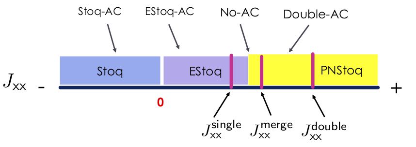
Figure 1: Stoquasticity of ${\mathcal{H}}^{\mathsf{XX\!-\!Sys}}(J_{\mathsf{xx}},G_{\mathsf{driver}},G)$ where ${\mathcal{H}}_{{\mathsf{XX}}}=J_{\mathsf{xx}}\sum_{ij\in{\mathsf{E}}(G_{\mathsf{driver}})}\sigma_{i}^{x}\sigma_{j}^{x}$. ${\mathcal{H}}^{\mathsf{XX\!-\!Sys}}(J_{\mathsf{xx}},G_{\mathsf{driver}},G)$ is Stoq(in blue) if $J_{\mathsf{xx}}<0$; it is EStoq(in purple) if $0<J_{\mathsf{xx}}<J^{\mathsf{transition}}_{\mathsf{xx}}$; and it is PNStoq(in yellow) if $J_{\mathsf{xx}}\geq J^{\mathsf{transition}}_{\mathsf{xx}}$. For ${\mathcal{H}}^{\mathsf{XX\!-\!Sys}}(J_{\mathsf{xx}},G_{\mathsf{driver}},G)$ described in Section 2.2, the system has a double-AC when $J_{\mathsf{xx}}\in(J^{\mathsf{merge}}_{\mathsf{xx}},J^{\mathsf{double}}_{\mathsf{xx}}]$ where $J^{\mathsf{merge}}_{\mathsf{xx}}\geq J^{\mathsf{transition}}_{\mathsf{xx}}$. As $J_{\mathsf{xx}}$ decreases from $J^{\mathsf{double}}_{\mathsf{xx}}$, the bridge between the two ACs shrinks, and the two ACs eventually merges, resulting in no AC, at $J^{\mathsf{merge}}_{\mathsf{xx}}$. Note that no AC does not necessarily imply that the gap is not small.

Recently, it has been claimed that for “typical” systems, the min-gap of the non-stoquastic Hamiltonian is smaller than its “de-signed” stoquastic counterpart [18]. However, we show by a counter-argument (in Observation 1 of Section 2.2) and a counter-example (see Figures 9 and 11) that the opposite is true when the non-stoquastic Hamiltonian is eventually stoquastic and an appropriate driver graph (which can be constructed efficiently) is taken into consideration. The driver graph is either not explicitly addressed or assumed to be the same as the problem graph in [18].

For the PNStoq, its ground state has both positive and negative amplitudes. It is this proper non-stoquasticity feature, which is exclusively quantum mechanics, that we will make use of. Furthermore, there are reasons to believe that PNStoq Hamiltonians (with $\mathsf{XX}$-driver Hamiltonians) are not VGP [16], and thus not QMC-simulable.

1.2 Preliminary and Notation

We now introduce some necessary notation. Let $|E_{k}(s)\rangle$ ($E_{k}(s)$ respectively) be the instantaneous eigenstate (energy respectively) of the system Hamiltonian ${\mathcal{H}}(s)$ in Eq.(1) at time $s\in[0,1]$, i.e., ${\mathcal{H}}(s)|E_{k}(s)\rangle=E_{k}(s)|E_{k}(s)\rangle$ for $k=0,1,\ldots 2^{N}-1,$ where $N$ is the number of qubits in the system. For convenience, we write $E_{k}\stackrel{{\scriptstyle\mathrm{def}}}{{=}}E_{k}(1)$ and $|E_{k}\rangle\stackrel{{\scriptstyle\mathrm{def}}}{{=}}|E_{k}(1)\rangle$ for the energy and state of the problem (final) Hamiltonian ${\mathcal{H}}_{\mathsf{problem}}={\mathcal{H}}(1)$. For convenience, we write $H_{P}={\mathcal{H}}_{\mathsf{problem}}$, and $H_{D}={\mathcal{H}}_{\mathsf{driver}}$, and let $\delta H=H_{P}-H_{D}$.

Let $2^{[N]}$ denote all possible bit strings of length $N$ which correspond to all possible states of the problem Hamiltonian. Each bit string corresponds to a subset of $\{0,1,...,N-1\}$ (the position with value 1 corresponds to the element in the subset). When there is no confusion, we use the subsets and the corresponding bit strings interchangeably. Thus, $2^{[N]}$ also represents all possible subsets of $\{0,1,...,N-1\}$, and $\{|k\rangle:k\in 2^{[N]}\}$ consists of all problem states (also known as the classical states). Note that the problem ground state$|E_{0}\rangle$ is in general not the same as the zero state $|0\rangle$.

We express the instantaneous eigenstates ($|E_{0}(s)\rangle,|E_{1}(s)\rangle$) in terms of the classical states:

$$\left\{\begin{array}[]{ll}|E_{0}(s)\rangle=\sum_{k=0}^{2^{N}-1}{\color[rgb]{1,0,0}c_{k}(s)}|k\rangle,&\sum_{k=0}^{2^{N}-1}|c_{k}(s)|^{2}=1\\ |E_{1}(s)\rangle=\sum_{k=0}^{2^{N}-1}{\color[rgb]{0,0,1}d_{k}(s)}|k\rangle,&\sum_{k=0}^{2^{N}-1}|d_{k}(s)|^{2}=1\end{array}\right.$$

That is, we have ${c_{k}(s)}=\langle E_{0}(s)|k\rangle$ and ${d_{k}(s)}=\langle E_{1}(s)|k\rangle$ for all $k<2^{N}$.

In general (in the proper non-stoquastic case), $c_{k}(s)$ can be positive or negative, and/or can change the sign during the evolution course. Since the squared overlap $|c_{k}(s)|^{2}$ would lose the sign of $c_{k}(s)$, we introduce the signed overlap, $\mathsf{sgn}(c_{k}(s))|c_{k}(s)|^{2}$. We will visualize our results using the signed overlaps whenever the signs are significant. In particular, the evolution of the signed overlaps of $c_{k}(s)$ and $d_{k}(s)$ will help us understand the formation of the anti-crossings during the quantum evolution.

For $A\subset 2^{[N]}$ (e.g. a set of local minima states), we denote the projection of the eigenstate $|E_{i}(s)\rangle$ onto $A$ by $|A_{i}(s)\rangle=\widehat{P}_{A}|E_{i}(s)\rangle$ where $\widehat{P}_{A}=\sum_{a\in A}|a\rangle\langle a|$ is the projection operator, and $|A_{i}(s)|=||A_{i}(s)||$ denotes its norm. For example, $|A_{0}(s)\rangle=\sum_{k\in A}c_{k}(s)|k\rangle$ and $|A_{0}(s)|=\sum_{k\in A}|c_{k}(s)|^{2}$; similarly for $|A_{1}(s)\rangle$ and $|A_{1}(s)|$ (with $c_{k}(s)$ replaced by $d_{k}(s)$).

Let $\Delta_{ij}(s)=E_{i}(s)-E_{j}(s)$ be the instantaneous spectral gap between the $i$th and $j$th energy levels, for $s\in[0,1]$.

Driver-dependent neighborhood and distance.

As in [4], we define the driver-dependent neighbourhood ${\mathsf{nbr}}_{H_{D}}(|k\rangle)=\{|q\rangle:|q\rangle=\mathsf{Op}_{i}(|k\rangle),i=0,\ldots,p\}$, where $H_{D}=\sum_{i=0}^{p}\mathsf{Op}_{i}$ is the driver Hamiltonian and $k,q\in 2^{[N]}$. By this definition, ${\mathsf{nbr}}_{{\mathcal{H}}_{\mathsf{X}}}$ consists of the single-bit flip neighbourhood of the state. For example, ${\mathsf{nbr}}_{{\mathcal{H}}_{\mathsf{X}}}(|101\rangle)=\{|10\underline{0}\rangle,|1\underline{1}1\rangle,|\underline{0}01\rangle\}$. Define ${\mathsf{nbr}}_{H_{D}}(L)=\cup_{l\in L}{\mathsf{nbr}}_{H_{D}}(|l\rangle)$.

Define ${\mathsf{dist}}_{H_{D}}(|k\rangle,|q)\rangle$ to be the number of $\mathsf{Op}$s in the minimum path between $|k\rangle$ and $|q\rangle$ (computational states). For $L,R\subset 2^{N}$, define ${\mathsf{dist}}_{H_{D}}(L,R)\stackrel{{\scriptstyle\mathrm{def}}}{{=}}\min_{l\in L,r\in R}{\mathsf{dist}}_{H_{D}}(|l\rangle,|r\rangle)$. For example, ${\mathsf{dist}}_{H_{X}}(L,R)$ is the minimum Hamming distance between sets in $L$ and $R$.

Sets $L$, $n(L)$, $\tilde{L}$, $\overline{L}$.

For $L,R\subset 2^{N}$, the space $2^{[N]}$ is partitioned to $\tilde{L}\cup\tilde{R}$, where $\tilde{L}=L\cup n(L)$ and $\tilde{R}=R\cup n(R)$. The set $n(L)$ ($n(R)$ resp.) consists of states that are driver-distance closer to $L$ than $R$ ($R$ than $L$ resp.). That is,

$$\begin{cases}n(L)=\{x\in 2^{[N]}:{\mathsf{dist}}_{H_{D}}(\{x\},L)\leq{\mathsf{dist}}_{H_{D}}(\{x\},R)\}\\ n(R)=\{x\in 2^{[N]}:{\mathsf{dist}}_{H_{D}}(\{x\},L)>{\mathsf{dist}}_{H_{D}}(\{x\},R)\}\\ \end{cases}$$

See Figure 2 for an illustration.

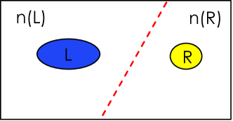
Figure 2: The space $2^{[N]}$ is partitioned to $\tilde{L}\cup\tilde{R}$, where $\tilde{L}=L\cup n(L)$ and $\tilde{R}=R\cup n(R)$.

We also denote $\overline{L}=L\cup{\mathsf{nbr}}_{H_{D}}(L)$ and $\overline{R}=R\cup{\mathsf{nbr}}_{H_{D}}(R)$. The set ${\mathsf{nbr}}_{H_{D}}(A)$ contains the low-energy neighboring-states (LENS) introduced in [4]. In particular, ${\mathsf{LENS}}(A)=\{k\in{\mathsf{nbr}}_{H_{D}}(A):\mathsf{energy}(k)\leq\mathsf{threshold}\}$, for some instance dependent $\mathsf{threshold}$.

The paper is organized as follows. We describe our results in Section 2. In Section 2.1, we give the definition of anti-crossing, and describe four characterizations of the AC, the necessary conditions for the formation of an AC, and the two formulae for computing the AC-gap. In Section 2.2, we describe our algorithm Dic-Dac-Doa. We conclude with our discussion in Section 3. The proofs are included in Section 4.

2 Results

2.1 Anti-crossing: A Tool for Design and Analysis of QA algorithm

2.1.1 New Defintion of Anti-Crossing

Informally, in the context of the quantum annealing, we define an anti-crossing between two consecutive levels with the following four conditions: (1) the anti-crossing point corresponds to a local minimum in the energy spectrum between the two interacting levels; (2) within the anti-crossing interval, all other energy levels are far away from the two interacting levels; (3) there are two small sets of “non-negligible” states involved in the anti-crossing; (4) a “sharp exchange” of the non-negligible states within a small width of the anti-crossing interval.

More formally, a new parametrization definition of an anti-crossing between the lowest two levels (which can be straightforwardly generalized to any two consecutive levels) during the evolution of ${\mathcal{H}}(s)$ in Eq. (1) is defined as follows.

Definition 2.1.

We say that there is an ${(L,R)\!\!-\!\!{\footnotesize\textsc{Anti-crossing}}}$ at $s_{\mbox{\!\tiny$\times$}}$ if there exists two disjoint subsets $L$ and $R$ ($\subset 2^{[N]}$), and $\delta>0$, $\gamma>0$ such that

(i)

For $s\in[s_{\mbox{\!\tiny$\times$}}-\delta,s_{\mbox{\!\tiny$\times$}}+\delta]$, $\Delta_{10}(s_{\mbox{\!\tiny$\times$}})\leq\Delta_{10}(s)$;

(ii)

For $s\in[s_{\mbox{\!\tiny$\times$}}-\delta,s_{\mbox{\!\tiny$\times$}}+\delta]$, $\Delta_{10}(s)<<\Delta_{k0}(s)$, for all $k>1$;

(iii)

Within the time interval $[s_{\mbox{\!\tiny$\times$}}-\delta,s_{\mbox{\!\tiny$\times$}}+\delta]$, both $|E_{0}(s)\rangle$ and $|E_{1}(s)\rangle$ are mainly composed of states from $L$ and $R$. More precisely, let $\widetilde{L}=L\cup n(L)$, $\widetilde{R}=R\cup n(R)$, such that all the possible states $2^{[N]}=\widetilde{L}\cup\widetilde{R}$, and $\widetilde{L}\cap\widetilde{R}=\emptyset$. For $s\in[s_{\mbox{\!\tiny$\times$}}-\delta,s_{\mbox{\!\tiny$\times$}}+\delta]$,

$$|E_{i}(s)\rangle=|\widetilde{L_{i}}(s)\rangle+|\widetilde{R_{i}}(s)\rangle\simeq|L_{i}(s)\rangle+|R_{i}(s)\rangle$$ (2)

where $|L_{i}(s)|+|R_{i}(s)|\in[1-\gamma,1]$ and $|n(L_{i})(s)|+|n(R_{i})(s)|\in[0,\gamma]$, $i=0,1$. (Recall: $|A_{0}(s)\rangle=\sum_{k\in A}c_{k}(s)|k\rangle$ and $|A_{1}(s)\rangle=\sum_{k\in A}d_{k}(s)|k\rangle$.)

(iv)

Before the anti-crossing at $s_{\mbox{\!\tiny$\times$}}^{-}\equiv s_{\mbox{\!\tiny$\times$}}-\delta$, $|E_{0}(s_{\mbox{\!\tiny$\times$}}^{-})\rangle\simeq|L_{0}(s_{\mbox{\!\tiny$\times$}}^{-})\rangle$ (or $|{L_{0}(s_{\mbox{\!\tiny$\times$}}^{-})}|\geq(1-\gamma)$), $|E_{1}(s_{\mbox{\!\tiny$\times$}}^{-})\rangle\simeq|R_{1}(s_{\mbox{\!\tiny$\times$}}^{-})\rangle$; after the anti-crossing at $s_{\mbox{\!\tiny$\times$}}^{+}\equiv s_{\mbox{\!\tiny$\times$}}+\delta$, $|E_{0}(s_{\mbox{\!\tiny$\times$}}^{+})\rangle\simeq|R_{0}(s_{\mbox{\!\tiny$\times$}}^{+})\rangle$, $|E_{1}(s_{\mbox{\!\tiny$\times$}}^{+})\rangle\simeq|L_{1}(s_{\mbox{\!\tiny$\times$}}^{+})\rangle$.

For convenience, we shall refer $(L,R)$ as the two arms of the anti-crossing (they appear in the left and right of each energy level). We shall refer $\delta$ as the AC-width, and ${\mathsf{dist}}_{H_{D}}(L,R)$ as the AC-distance. One can take the AC-width to be the $\delta$ such that the minimum of the four “corner overlaps” is maximized, i.e. $\delta=\max_{\xi>0}\min\{\langle E_{0}(s_{\mbox{\!\tiny$\times$}}-\xi)|L_{0}(s_{\mbox{\!\tiny$\times$}}-\xi)\rangle,\langle E_{1}(s_{\mbox{\!\tiny$\times$}}-\xi)|R_{1}(s_{\mbox{\!\tiny$\times$}}-\xi)\rangle,\langle E_{0}(s_{\mbox{\!\tiny$\times$}}+\xi)|R_{0}(s_{\mbox{\!\tiny$\times$}}+\xi)\rangle,\langle E_{1}(s_{\mbox{\!\tiny$\times$}}+\xi)|L_{1}(s_{\mbox{\!\tiny$\times$}}+\xi)\rangle\}$. In general, we require $\gamma$ to be near $1$. Sometimes it is possible to increase $\gamma$ by enlarging $L$ and/or $R$ such that ${(L^{*},R^{*})\!\!-\!\!{\footnotesize\textsc{Anti-crossing}}}$ is an anti-crossing with a larger $\gamma$ (for the same $\delta$), where $L\subseteq L^{*},R\subseteq R^{*}$. A figure depicting an ${(L,R)\!\!-\!\!{\footnotesize\textsc{Anti-crossing}}}$ is shown in Figure 3.

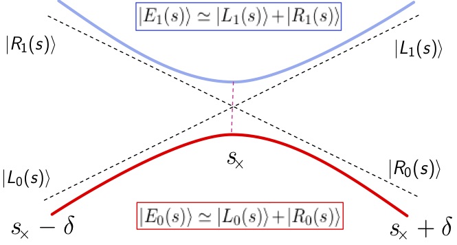
(a)

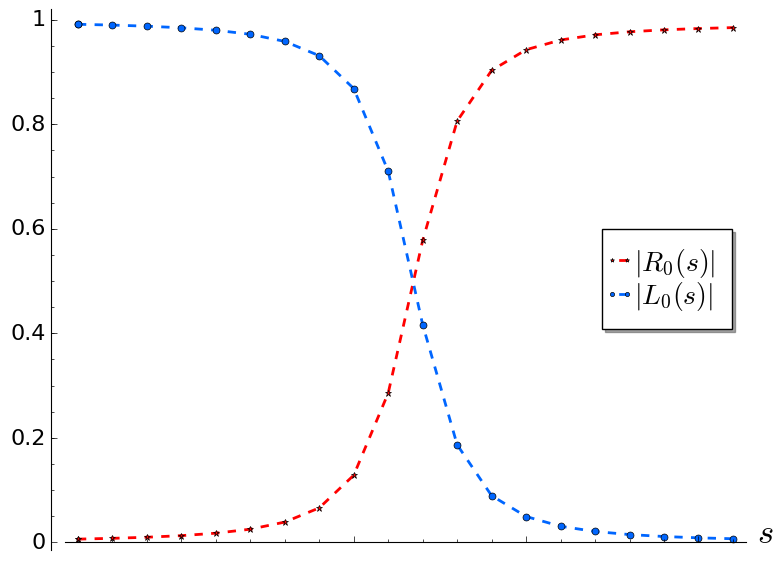
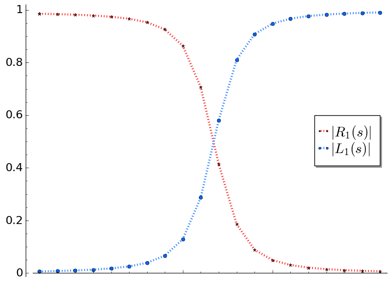
(b)

Figure 3: An ${(L,R)\!\!-\!\!{\footnotesize\textsc{Anti-crossing}}}$ at $s_{\mbox{\!\tiny$\times$}}$. (a) Within the time interval $[s_{\mbox{\!\tiny$\times$}}-\delta,s_{\mbox{\!\tiny$\times$}}+\delta]$, both $|E_{0}(s)\rangle$ and $|E_{1}(s)\rangle$ are mainly composed of states from $L$ and $R$. That is, $|E_{0}(s)\rangle\simeq|L_{0}(s)\rangle+|R_{0}(s)\rangle$ and $|E_{1}(s)\rangle\simeq|L_{1}(s)\rangle+|R_{1}(s)\rangle$ where $|A_{i}(s)\rangle=\sum_{k\in A}f^{i}_{k}(s)|k\rangle$, with $f^{0}_{k}=c_{k},f^{1}_{k}=d_{k}$, $A\in\{L,R\}$, $i=0,1$. (b) When $s$ goes from $s_{\mbox{\!\tiny$\times$}}-\delta$ to $s_{\mbox{\!\tiny$\times$}}+\delta$ , the state $|E_{0}(s)\rangle$ shifts from $L$ to $R$ while $|E_{1}(s)\rangle$ shifts from $R$ to $L$: $|L_{0}(s)|\downarrow$, $|R_{0}(s)|\uparrow$ while $|R_{1}(s)|\downarrow$, $|L_{1}(s)|\uparrow$, where $|A_{i}(s)|=\sum_{k\in A}|f^{i}_{k}(s)|^{2}$ is the total magnitude in $A_{i}(s)$, for $A\in\{L,R\}$, $i=0,1$. The figures show the evolution of $|L_{0}(s)|$ and $|R_{0}(s)|$ (left) and $|L_{1}(s)|$ and $|R_{1}(s)|$ (right) within the interval $[s_{\mbox{\!\tiny$\times$}}-\delta,s_{\mbox{\!\tiny$\times$}}+\delta]$.

By definition, there is an exchange between the same arm of the two levels. For $\epsilon_{v}>0$, we say the ${(L,R)\!\!-\!\!{\footnotesize\textsc{Anti-crossing}}}$ is a $(1-\epsilon_{v})$-full-exchange anti-crossing if

$$\begin{cases}|c_{k}(s_{\mbox{\!\tiny$\times$}}^{-})|\doteq_{\epsilon_{v}}|d_{k}(s_{\mbox{\!\tiny$\times$}}^{+})|\mbox{ for all }k\in\tilde{L}\\ |c_{k}(s_{\mbox{\!\tiny$\times$}}^{+})|\doteq_{\epsilon_{v}}|d_{k}(s_{\mbox{\!\tiny$\times$}}^{-})|\mbox{ for all }k\in\tilde{R}\\ \end{cases}$$ (3)

such that

$$\begin{cases}|\langle L_{0}(s_{\mbox{\!\tiny$\times$}}^{-})|L_{1}(s_{\mbox{\!\tiny$\times$}}^{+})\rangle|\approx|L_{0}(s_{\mbox{\!\tiny$\times$}}^{-})|\approx|L_{1}(s_{\mbox{\!\tiny$\times$}}^{+})|\\ |\langle R_{1}(s_{\mbox{\!\tiny$\times$}}^{-})|R_{0}(s_{\mbox{\!\tiny$\times$}}^{+})\rangle|\approx|R_{1}(s_{\mbox{\!\tiny$\times$}}^{-})|\approx|R_{0}(s_{\mbox{\!\tiny$\times$}}^{+})|\end{cases}$$ (4)

where $A\doteq_{\epsilon_{v}}B$ means $|A-B|\leq\epsilon_{v}$, This condition in Eq. (4) is required to derive both the SAS property in (C4) in Section 2.1.2 and the necessary conditions (Eq. (8) in Section 2.1.3.

In this paper, we fix a small $\epsilon_{v}>0$, and assume an ${(L,R)\!\!-\!\!{\footnotesize\textsc{Anti-crossing}}}$ satisfies this condition when we do not mention explicitly.

The earlier definition in [4] is a special case with $L=\{|E_{1}\rangle\}$ (corresponds to $|\mathsf{FS}\rangle\stackrel{{\scriptstyle\mathrm{def}}}{{=}}|E_{1}\rangle$), and $R=\{|E_{0}\rangle\}$ (corresponds to $|\mathsf{GS}\rangle\stackrel{{\scriptstyle\mathrm{def}}}{{=}}|E_{0}\rangle$), without explicitly requiring the SAS property within $\epsilon$ at $s_{\mbox{\!\tiny$\times$}}$ in the definition. We re-introduce the “negligible” sets $n(L)$ and $n(R)$ back to the definition for the purpose of computing the $\mathsf{AC\!\!-\!\!Gap}$. The coefficients of states in $n(L),n(R)$ are “negligible” but not “vanishing”. Indeed, we shall show that the “negligible” states are what contribute to the gap size. (Similar to the idea that it is the high-order correction terms in the perturbation formula that contribute to the perturbative-crossing gap size.)

2.1.2 New Characterizations of the Anti-crossing

We derive some useful characteristics of the AC based on the perturbation theory. The derivation is based on the idea that in the neighborhood of $s_{\mbox{\!\tiny$\times$}}$ the behavior of these two energy levels can be approximately computed by non-degenerate perturbation theory for the two lowest energy levels while the other energy levels are far away enough to be neglected.

Proposition 2.2.

An ${(L,R)\!\!-\!\!{\footnotesize\textsc{Anti-crossing}}}$ has the following four properties.

(C1)

(”Hyperbolic-like curves”) The two energy levels form two opposite parabolas around $s_{\mbox{\!\tiny$\times$}}$:

$$\begin{cases}E_{1}(s_{\mbox{\!\tiny$\times$}}+\lambda)\doteq\alpha\lambda^{2}+\beta_{1}\lambda+E_{1}(s_{\mbox{\!\tiny$\times$}})\\ E_{0}(s_{\mbox{\!\tiny$\times$}}+\lambda)\doteq-\alpha\lambda^{2}+\beta_{0}\lambda+E_{0}(s_{\mbox{\!\tiny$\times$}})\end{cases}$$ (5)

for $\lambda\in[-\delta,\delta]$, where $\alpha>0$, $\alpha=\frac{|\langle E_{1}(s_{\mbox{\!\tiny$\times$}})|\delta H|E_{0}(s_{\mbox{\!\tiny$\times$}})\rangle|^{2}}{\Delta_{10}(s_{\mbox{\!\tiny$\times$}})}>0$ and $\beta_{1}\simeq\beta_{0}$. Thus, we have $E_{1}(s_{\mbox{\!\tiny$\times$}}+\lambda)-E_{0}(s_{\mbox{\!\tiny$\times$}}+\lambda)\doteq 2\alpha\lambda^{2}+\Delta_{10}(s_{\mbox{\!\tiny$\times$}})$. The gap at the AC point is a local minimum of the gap spectrum.

(C2)

(”States-exchange”) When $s$ goes from $s_{\mbox{\!\tiny$\times$}}-\delta$ to $s_{\mbox{\!\tiny$\times$}}+\delta$ , the state $|E_{0}(s)\rangle$ shifts from $L$ to $R$ while $|E_{1}(s)\rangle$ shifts from $R$ to $L$: $|c_{l}(s)|\downarrow$ for all $l\in L$, $|c_{r}(s)|\uparrow$ for all $r\in R$; while $|d_{r}(s)|\downarrow$ for all $r\in R$, $|d_{l}(s)|\uparrow$ for all $l\in L$, where $\downarrow$ denotes decreasing and $\uparrow$ denotes increasing. In particular, for $s:s_{\mbox{\!\tiny$\times$}}-\delta\leadsto s_{\mbox{\!\tiny$\times$}}+\delta$, $|L_{0}(s)|\downarrow$, $|R_{0}(s)|\uparrow$ while $|R_{1}(s)|\downarrow$, $|L_{1}(s)|\uparrow$.

(C3)

(“Opposite signs”) One arm is of the same sign in the two states; the other arm is of the opposite sign in the two states. That is, it is either

$$\begin{cases}L_{0}\mbox{ and }L_{1}\mbox{ in the same sign: }\mathsf{sgn}(c_{l}(s))\mathsf{sgn}(d_{l}(s))=+1\mbox{ for all }l\in L\\ R_{0}\mbox{ and }R_{1}\mbox{ in the opposite sign: }\mathsf{sgn}(c_{r}(s))\mathsf{sgn}(d_{r}(s))=-1\mbox{ for all }r\in R\end{cases}$$ (6)

or the reverse.

(C4)

(“Symmetry-and-anti-symmetry(SAS) at $s_{\mbox{\!\tiny$\times$}}$”)

$$\begin{cases}c_{l}(s_{\mbox{\!\tiny$\times$}})\doteq d_{l}(s_{\mbox{\!\tiny$\times$}})\mbox{ for }l\in\widetilde{L}\\ c_{r}(s_{\mbox{\!\tiny$\times$}})\doteq-d_{r}(s_{\mbox{\!\tiny$\times$}})\mbox{ for }r\in\widetilde{R}\end{cases}or\begin{cases}c_{l}(s_{\mbox{\!\tiny$\times$}})\doteq-d_{l}(s_{\mbox{\!\tiny$\times$}})\mbox{ for }l\in\widetilde{L}\\ c_{r}(s_{\mbox{\!\tiny$\times$}})\doteq d_{r}(s_{\mbox{\!\tiny$\times$}})\mbox{ for }r\in\widetilde{R}\end{cases}$$ (7)

Thus, we have $|\widetilde{L}(s_{\mbox{\!\tiny$\times$}})\rangle\doteq|\widetilde{L_{0}}(s_{\mbox{\!\tiny$\times$}})\rangle\doteq(+/-)|\widetilde{L_{1}}(s_{\mbox{\!\tiny$\times$}})\rangle$ and $|\widetilde{R}(s_{\mbox{\!\tiny$\times$}})\rangle\doteq|\widetilde{R_{0}}(s_{\mbox{\!\tiny$\times$}})\rangle\doteq(-/+)|\widetilde{R_{1}}(s_{\mbox{\!\tiny$\times$}})\rangle$, i.e.

$$(*)\begin{cases}|E_{0}(s_{\mbox{\!\tiny$\times$}})\rangle\doteq|\widetilde{L}(s_{\mbox{\!\tiny$\times$}})\rangle{\color[rgb]{1,0,0}+}|\widetilde{R}(s_{\mbox{\!\tiny$\times$}})\rangle\\ |E_{1}(s_{\mbox{\!\tiny$\times$}})\rangle\doteq|\widetilde{L}(s_{\mbox{\!\tiny$\times$}})\rangle{\color[rgb]{1,0,0}-}|\widetilde{R}(s_{\mbox{\!\tiny$\times$}})\rangle\end{cases}\mbox{ or }(**)\begin{cases}|E_{0}(s_{\mbox{\!\tiny$\times$}})\rangle\doteq|\widetilde{L}(s_{\mbox{\!\tiny$\times$}})\rangle+|\widetilde{R}(s_{\mbox{\!\tiny$\times$}})\rangle\\ |E_{1}(s_{\mbox{\!\tiny$\times$}})\rangle\doteq{\color[rgb]{1,0,0}-}|\widetilde{L}(s_{\mbox{\!\tiny$\times$}})\rangle+|\widetilde{R}(s_{\mbox{\!\tiny$\times$}})\rangle\end{cases}$$

Furthermore, $|A_{i}(s_{\mbox{\!\tiny$\times$}})|\in[1/2-\gamma/2,1/2+\gamma/2]$, for $A\in\{L,R\}$, $i=0,1$.

AC-signature.

We refer to the two reverse curves in the Property (C2) as the “AC-signature” to describe the “sharp exchange” between the ground state and the first excited state at the anti-crossing interval. This is more general than the Hamming weight operator $<\!HW\!>$ (when the problem ground state is assumed to be the zero vector) introduced in [8] that describes the changes of the ground state wavefunction (without describing the reverse changes of the first excited state wavefunction).

Significance of the Sign.

It is worthwhile to emphasize the signs of the coefficients of the two arms in Property (C3) are critical. There are two possible cases and are depicted in Figure 4. The two anti-crossings can be connected/bridged through a common arm which is of the opposite sign. That is, the bridge consists of both positive and negative amplitudes (requiring the proper-non-stoquastic condition). Furthermore, since one arm of the AC must be in the opposite sign, if the ground state only allows the positive sign (as in the stoquastic case), the possible combinations (+/+, -/+) will be less in the stoquastic case than the possible combinations (+/+, -/-, -/+, +/-) in the non-stoquastic cases. This partially explains why one would observe more ACs in the non-stoquastic case.

$$\begin{array}[h]{cc}\includegraphics[width=138.76157pt]{NS-1AC-Same-L1.png}&\includegraphics[width=138.76157pt]{NS-1AC-Diff-R1.png}\\ (a)L_{1}:|d_{l}(s)|\uparrow&(c)R_{1}:|d_{r}(s)|\downarrow\\ \includegraphics[width=138.76157pt]{NS-1AC-Same-L0.png}&\includegraphics[width=138.76157pt]{NS-1AC-Diff-R0.png}\\ (b)L_{0}:|c_{l}(s)|\downarrow&(d)R_{0}:|c_{r}(s)|\uparrow\\ \hline\cr\end{array}$$

$$\begin{array}[h]{cc}\includegraphics[width=138.76157pt]{NS-Diff-L1.png}&\includegraphics[width=138.76157pt]{NS-Same-R1.png}\\ (e)L^{\prime}_{1}:|d_{l}(s)|\uparrow&(g)R^{\prime}_{1}:|d_{r}(s)|\downarrow\\ \includegraphics[width=138.76157pt]{NS-Diff-L0.png}&\includegraphics[width=138.76157pt]{NS-Same-R0.png}\\ (f)L^{\prime}_{0}:|c_{l}(s)|\downarrow&(h)R^{\prime}_{0}:|c_{r}(s)|\uparrow\\ \hline\cr\end{array}$$

Figure 4: (Above)$L_{1}$ in (a) and $L_{0}$ in (b) in the same sign: $\mathsf{sgn}(c_{l})\mathsf{sgn}(d_{l})=+1\forall l\in L$; $R_{1}$ in (c) and $R_{0}$ in (d) in the different sign: $\mathsf{sgn}(c_{r})\mathsf{sgn}(d_{r})=-1\forall r\in R$. (Below) $L^{\prime}_{1}$ in (e) and $L^{\prime}_{0}$ in (f) in the different sign; $R^{\prime}_{1}$ in (g) and $R^{\prime}_{0}$ in (h) in the same sign. These are examples from a bridged double-AC: ${(L,R)\!\!-\!\!{\footnotesize\textsc{Anti-crossing}}}$ and ${(L^{\prime},R^{\prime})\!\!-\!\!{\footnotesize\textsc{Anti-crossing}}}$ where $R=L^{\prime}$ is the common arm of the opposite sign which is a necessary condition for a bridged double-AC to be formed.

2.1.3 Necessary Conditions for the Formation of the Anti-crossing

In this section we derive the necessary conditions for the formation of an ${(L,R)\!\!-\!\!{\footnotesize\textsc{Anti-crossing}}}$.

Theorem 2.3.

The necessary conditions for an ${(L,R)\!\!-\!\!{\footnotesize\textsc{Anti-crossing}}}$ at $s_{\mbox{\!\tiny$\times$}}$ with width $\delta$ are:

$$\begin{cases}{\langle{\delta H}\rangle}_{|E_{0}(s_{\mbox{\!\tiny$\times$}}^{-})\rangle}-{\langle{\delta H}\rangle}_{|E_{1}(s_{\mbox{\!\tiny$\times$}}^{-})\rangle}\approx 2\eta^{2}\frac{\delta}{\Delta_{01}(s_{\mbox{\!\tiny$\times$}})}\\ {\langle{\delta H}\rangle}_{|E_{1}(s_{\mbox{\!\tiny$\times$}}^{+})\rangle}-{\langle{\delta H}\rangle}_{|E_{0}(s_{\mbox{\!\tiny$\times$}}^{+})\rangle}\approx 2\eta^{2}\frac{\delta}{\Delta_{01}(s_{\mbox{\!\tiny$\times$}})}\end{cases}$$ (8)

where $\eta=\langle E_{1}(s_{\mbox{\!\tiny$\times$}})|\delta H|E_{0}(s_{\mbox{\!\tiny$\times$}})\rangle$ and ${\langle{\delta H}\rangle}_{|\psi\rangle}\stackrel{{\scriptstyle\mathrm{def}}}{{=}}\langle\psi|\delta H|\psi\rangle$. (Recall: $\delta H=H_{P}-H_{D}$.)

In particular, the necessary conditions described by $L,R$ are approximately:

$$\begin{cases}{\langle{\delta H}\rangle}_{L_{0},s_{\mbox{\!\tiny$\times$}}^{-}}>{\langle{\delta H}\rangle}_{R_{1},s_{\mbox{\!\tiny$\times$}}^{-}}\\ {\langle{\delta H}\rangle}_{L_{1},s_{\mbox{\!\tiny$\times$}}^{+}}>{\langle{\delta H}\rangle}_{R_{0},s_{\mbox{\!\tiny$\times$}}^{+}}\end{cases}$$ (9)

where ${\langle{\delta H}\rangle}_{|E_{i}(s^{*})\rangle}$ is approximated by ${\langle{\delta H}\rangle}_{A_{i},s^{*}}\stackrel{{\scriptstyle\mathrm{def}}}{{=}}\langle A_{i}(s^{*})|\delta{\mathcal{H}}|A_{i}(s^{*})\rangle$ when $|E_{i}(s^{*})\rangle\simeq|A_{i}(s^{*})\rangle$, for $i\in\{0,1\}$, $A\in\{L,R\},s^{*}\in\{s_{\mbox{\!\tiny$\times$}}^{-},s_{\mbox{\!\tiny$\times$}}^{+}\}$.

Since $\delta H=H_{P}-H_{D}$, when ${\langle{H_{P}}\rangle}_{L_{i},s^{*}}\approx{\langle{H_{P}}\rangle}_{R_{\overline{i}},s^{*}}$, for $i\in\{0,1\}$, $s^{*}\in\{s_{\mbox{\!\tiny$\times$}}^{-},s_{\mbox{\!\tiny$\times$}}^{+}\}$, the necessary conditions in Eq. (9) become ${\langle{-H_{D}}\rangle}_{L_{i},s^{*}}>{\langle{-H_{D}}\rangle}_{R_{\overline{i}},s^{*}}$. When there is no confusion, we drop the subscripts $i$ and $\overline{i}$ of $L,R$. When $H_{D}=H_{X}$, ${\langle{-H_{X}}\rangle}_{A,s^{*}}\approx\langle\overline{A}(s^{*})|\sum_{i}\sigma_{i}^{x}|\overline{A}(s^{*})\rangle$ is approximated by the overlap between $A$ and ${\mathsf{LENS}}(A)$. Thus the condition that ${\langle{-H_{X}}\rangle}_{L,s^{*}}>{\langle{-H_{X}}\rangle}_{R,s^{*}}$ would mean that $L$ has more LENS than $R$ as observed in [4]. Furthermore, we show that with some extra conditions, the necessary conditions are also sufficient. We also compare the necessary conditions with the arguments of the anti-crossing presented in the AQA algorithm for random Exact-Cover 3 instances by Altshuler et al in [12]. In our subsequent work, we will further elaborate these results.

Corollary 2.4.

The $\mathsf{AC\!\!-\!\!Gap}$ of an ${(L,R)\!\!-\!\!{\footnotesize\textsc{Anti-crossing}}}$ at $s_{\mbox{\!\tiny$\times$}}$ with width $\delta$ is given by

$$\Delta_{10}(s_{\mbox{\!\tiny$\times$}})\approx\begin{cases}2\eta^{2}\frac{\delta}{{\langle{\delta H}\rangle}_{|E_{0}(s_{\mbox{\!\tiny$\times$}}^{-})\rangle}-{\langle{\delta H}\rangle}_{|E_{1}(s_{\mbox{\!\tiny$\times$}}^{-})\rangle}}\\ 2\eta^{2}\frac{\delta}{{\langle{\delta H}\rangle}_{|E_{1}(s_{\mbox{\!\tiny$\times$}}^{+})\rangle}-{\langle{\delta H}\rangle}_{|E_{0}(s_{\mbox{\!\tiny$\times$}}^{+})\rangle}}\end{cases}$$ (10)

The above corollary follows directly from Eq.(8). The equation of $\mathsf{AC\!\!-\!\!Gap}$ in Eq. (10) provides a description how the $\mathsf{AC\!\!-\!\!Gap}$ depends on the two factors: the numerator $\delta$ (anti-crossing width) and the difference between $L$ and $R$ in the denominator. This will give us as a tool to study the effect on the gap size (without actually computing the gap size) by analyzing how the parameters of the anti-crossing evolve as we vary one parameter in the system Hamiltonian, including either the parameters in the problem Hamiltonian or the $\mathsf{XX}$-coupler strength in the driver Hamiltonian. In particular, we use Corollary 2.4 to justify the Observation 1 in Section 2.2.

2.1.4 $\mathsf{AC\!\!-\!\!Gap}$ Bound

In this section we derive the analytical $\mathsf{AC\!\!-\!\!Gap}$ bound for the anti-crossing that satisfies the SAS properties (for a small $\epsilon_{v}$) and also large $\gamma$ (such that the corresponding $L,R$ are taking as large as possible).

Theorem 2.5.

Suppose that $R$ consists of the problem ground state $|\mathsf{GS}\rangle$ and $L$ consists of the lowest few almost degenerate excited states. Then $\mathsf{AC\!\!-\!\!Gap}$ $\Delta_{10}(s_{\mbox{\!\tiny$\times$}})=\Theta(\zeta^{{\mathsf{dist}}_{H_{D}}(L,R)})$ where $0<\zeta<1$ and ${\mathsf{dist}}_{H_{D}}(L,R)$ is the driver-distance between $L$ and $R$ (referred to as the AC-distance).

Remark. The ${\mathsf{AC\!\!-\!\!Gap}}{}$ is necessarily exponentially small (in the AC-distance), however, it is not necessarily true that every exponentially small (even in the problem size) gap corresponds to an anti-crossing defined here. For example, it is not clear if the exponential small gap example presented in [19] corresponds to our anti-crossing because they only show that there exists an excited state whose energy is close to the ground energy level and thus condition (ii) in our definition is not necessarily satisfied. A possible future work is to generalize the AC definition between one energy level and one narrow band of closely together energy levels.

2.2 Quantum Speedup by Dic-Dac-Doa

MWIS Problem.

We use the NP-hard maximum-weighted independent set (MWIS) as our model problem. See, e.g. [25] for a recent classical algorithm for MWIS. We make use of the structure of maximal independent sets to construct the driver graph. As described in [4], MWIS and Ising problem can be efficiently reduced to each other. The MWIS-Ising Hamiltonian is specified by a problem graph $G$ and a weight vector $w$ on its vertices and a $J_{\mathsf{penalty}}$ (In our examples in this paper, we assume $J_{\mathsf{penalty}}=4$ when we omit to mention). The formulae for computing the corresponding $\{h,J\}$ are also described in the Appendix.

2.2.1 An illustrative Example

An MWIS graph with 9 weighted vertices is depicted in Figure 5. The global minimum corresponds to the maximum independent set $\{2,5,8\}$ with total weight of $4.02$. $G$ has 8 local minima, $\{\{v_{1},v_{2},v_{3}\}:v_{1}\in\{0,1\},v_{2}\in\{3,4\},v_{3}\in\{5,6\}\}$, corresponding to the 8 maximal independent sets, with total weights ranging from $3.70$ to $3.95$. This graph can be scaled to a graph of $3n$ vertices, where the global minimum consists of $n$ vertices, while there are $2^{n}$ local minima formed by $n$ independent-cliques.

$$\begin{array}[h]{cc}\includegraphics[width=195.12767pt]{Q9-graph.pdf}&\includegraphics[width=195.12767pt]{Q12-graph.pdf}\\ (a)&(b)\end{array}$$

Figure 5: (a) An MWIS problem graph $G$ with 9 weighted vertices (edges are in black and red). The global minimum corresponds to the maximum independent set $\{2,5,8\}$ (in yellow) with total weight of $4.02$. $G$ has 8 local minima, $L=\{\{v_{1},v_{2},v_{3}\}:v_{1}\in\{0,1\},v_{2}\in\{3,4\},v_{3}\in\{6,7\}\}$, with weights ranging from $3.70$ to $3.95$. The local-minima subgraph $G|_{L}$ consists of 3 disjoint cliques (edges in red) : $\{\{0,1\},\{3,4\},\{6,7\}\}$. This graph can be scaled to a graph of $3n$ vertices, where the global minimum consists of $n$ yellow vertices, while there are $2^{n}$ local minima formed by $n$ independent-cliques. (b) An MIS graph $G^{\prime}$ with 12 weighted vertices (with 3 extra vertices from $G$ in (a)). The global minimum is $\{2,5,8,9\}$ (in yellow). There are three independent-cliques that form the local minima, $L=\{\{v_{1},v_{2},v_{3}\}:v_{1}\in\{0,1,9\},v_{2}\in\{3,4,10\},v_{3}\in\{6,7\}\}$. The edges in $G^{\prime}|_{L}$ are in red.

We will compare the evolution of stoquastic ${\mathcal{H}}^{\mathsf{TFIM}}(G)$ with the evolutions of ${\mathcal{H}}^{\mathsf{XX\!-\!Sys}}(J_{\mathsf{xx}},G_{\mathsf{driver}},G)$ for various values of $J_{\mathsf{xx}}$ for the weighted graph $G$ in Figure 5. We use three metrics to compare the evolutions of the different algorithms: (1) gap-spectrum, shown in Figure 6; (2) AC-signature (total overlaps of the two arms with the ground state and the first excited state wavefunctions), shown in Figure 7; (3) Signed overlaps (of the lowest seven problem states with the ground state and the first excited state wavefunctions), shown in Figure 8.

$$\begin{array}[h]{cc}\includegraphics[width=164.77771pt]{Q9-X-mg.png}&\includegraphics[width=164.77771pt]{Q9-XX-08Jxx-mg.png}\\ (a){\mathcal{H}}^{\mathsf{TFIM}}(G)&(b){\mathcal{H}}^{\mathsf{XX\!-\!Sys}}(J_{\mathsf{xx}},G_{\mathsf{driver}},G),J_{\mathsf{xx}}=-0.8,G_{\mathsf{driver}}=G|_{L}\\ \hline\cr\\ \includegraphics[width=164.77771pt]{Q9-NS-08Jxx-mg+zoom.jpeg}&\includegraphics[width=164.77771pt]{Q9-NS-G-mg+LR.jpeg}\\ (c){\mathcal{H}}^{\mathsf{XX\!-\!Sys}}(J_{\mathsf{xx}},G_{\mathsf{driver}},G),J_{\mathsf{xx}}=+0.8,G_{\mathsf{driver}}=G|_{L}&(d){\mathcal{H}}^{\mathsf{XX\!-\!Sys}}(J_{\mathsf{xx}},G_{\mathsf{driver}},G),J_{\mathsf{xx}}=+0.8,G_{\mathsf{driver}}=G\\ \hline\cr\\ \includegraphics[width=164.77771pt]{Q12-G1-08Jxx-zoom.jpeg}&\includegraphics[width=164.77771pt]{Q12-G1-11Jxx-ann.jpeg}\\ (e){\mathcal{H}}^{\mathsf{XX\!-\!Sys}}(J_{\mathsf{xx}},G_{\mathsf{driver}},G^{\prime}),J_{\mathsf{xx}}=+0.8,G_{\mathsf{driver}}=G|_{L}&(f){\mathcal{H}}^{\mathsf{XX\!-\!Sys}}(J_{\mathsf{xx}},G_{\mathsf{driver}},G^{\prime}),J_{\mathsf{xx}}=+1.1,G_{\mathsf{driver}}=G|_{L}\\ \hline\cr\end{array}$$

Figure 6: The gap-spectrum comparison of ${\mathcal{H}}^{\mathsf{TFIM}}(G)$ with ${\mathcal{H}}^{\mathsf{XX\!-\!Sys}}(J_{\mathsf{xx}},G_{\mathsf{driver}},G)$ for the weighted graph $G$ shown in Figure 5(a). There is one local minimum in the gap-spectrum for the stoquastic Hamiltonians in (a) and (b). There are three local minima in the gap-spectrum of the proper non-stoquastic Hamiltonian, where $G_{\mathsf{driver}}=G|_{L}$, in (c). The last two local minima in (c) correspond to two bridged anti-crossings (a double-AC) with a large second-level gap (in green). In (d), where $G_{\mathsf{driver}}=G$, there is no longer a double-AC, but one AC (the first minimum corresponds to a non-AC local minimum). In (e) and (f), the problem graph is $G^{\prime}$ in Figure 5(b). There is a double-AC with a large second-level gap for $J_{\mathsf{xx}}=+0.8$ in (e); there are three nested double-ACs when $J_{\mathsf{xx}}=+1.1$ in (f), with a large gap from the 4th-level (in magenta).

$$\begin{array}[h]{cc}L/R\mbox{ Overlap with }$$|E_{0}(s)\rangle$$&L/R\mbox{ Overlap with }$$|E_{1}(s)\rangle$$\\ \includegraphics[width=173.44534pt]{Q9-X-LR0star.jpeg}&\includegraphics[width=173.44534pt]{Q9-X-LR1star.jpeg}\\ (a){\mathcal{H}}_{X}:{(L^{*},R^{*})\!\!-\!\!{\footnotesize\textsc{Anti-crossing}}}&\\ \hline\cr\\ \includegraphics[width=173.44534pt]{Q9-XX-08Jxx-LR0.png}&\includegraphics[width=173.44534pt]{Q9-XX-08Jxx-LR1.jpeg}\\ (b){\mathcal{H}}_{{\mathsf{XX}}},J_{\mathsf{xx}}=-0.8:{(L,R)\!\!-\!\!{\footnotesize\textsc{Anti-crossing}}}&\\ \hline\cr\\ \includegraphics[width=173.44534pt]{Q9-NS-08Jxx-LR0star.jpeg}&\includegraphics[width=173.44534pt]{Q9-NS-08Jxx-LR1star.jpeg}\\ (c){\mathcal{H}}_{{\mathsf{XX}}},J_{\mathsf{xx}}=+0.8:\mbox{two bridged anti-crossings}\\ \hline\cr\end{array}$$

Figure 7: The “AC-signature” comparison of ${\mathcal{H}}^{\mathsf{TFIM}}(G)$ with ${\mathcal{H}}^{\mathsf{XX\!-\!Sys}}(J_{\mathsf{xx}},G_{\mathsf{driver}},G)$ for the weighted graph $G$ in Figure 5(a). The L/R overlaps with $|E_{0}(s)\rangle$ are shown in left, and with $|E_{1}(s)\rangle$ are shown in right, where $L^{*}=L\cup{\mathsf{nbr}}_{H_{D}}(L),R^{*}=R\cup{\mathsf{nbr}}_{H_{D}}(R)$. In both (b) and (c), $G_{\mathsf{driver}}=G|_{L}$. In (c), there is a double-AC : (1st AC) ${(R^{*},L)\!\!-\!\!{\footnotesize\textsc{Anti-crossing}}}$ at $\sim 0.5$ and (2nd AC) ${(L,R)\!\!-\!\!{\footnotesize\textsc{Anti-crossing}}}$ at $\sim 0.7$.

$$\begin{array}[h]{cc}\mbox{Signed overlap with }$$|E_{0}(s)\rangle$$&\mbox{Signed overlap with }$$|E_{1}(s)\rangle$$\\ \includegraphics[width=186.45341pt]{Q9+Jxx-C-y-1.jpeg}&\includegraphics[width=186.45341pt]{Q9+Jxx0-D.png}\\ (a){\mathcal{H}}^{\mathsf{TFIM}}(G):{(L,R)\!\!-\!\!{\footnotesize\textsc{Anti-crossing}}}&\\ \hline\cr\\ \includegraphics[width=186.45341pt]{Q9+Jxx08-C.jpeg}&\includegraphics[width=186.45341pt]{Q9+Jxx08-D.jpeg}\\ \includegraphics[width=173.44534pt]{Q9+Jxx08-C-bridge.jpeg}&\includegraphics[width=173.44534pt]{Q9-bridge-sets.jpeg}\\ (b)J_{\mathsf{xx}}=+0.8:L\mbox{ is splited into }L^{+}\mbox{ and }L^{-}\\ \hline\cr\\ \end{array}$$

Figure 8: The signed-overlap comparison of ${\mathcal{H}}^{\mathsf{TFIM}}(G)$ with ${\mathcal{H}}^{\mathsf{XX\!-\!Sys}}(J_{\mathsf{xx}},G_{\mathsf{driver}},G)$ for the weighted graph $G$ in Figure 5(a). Signed Overlap of the seven lowest energy levels with $|E_{0}(s)\rangle$ (shown in left) and with $|E_{1}(s)\rangle$ (shown in right). In (b), $G_{\mathsf{driver}}=G|_{L}$. $L$ is split into $L^{+}$ and $L^{-}$. There is exactly one XX-coupler between each state in $L^{+}$ and $L^{-}$. There is either zero or more than one XX-coupler within $L^{+}$ (or $L^{-}$).

2.2.2 Local Minima Subgraph and Driver Graph $G_{\mathsf{driver}}$

Local minima subgraph with a special independent-cliques (IC) structure.

Let $L=\{l_{1},l_{2},\ldots,l_{m}\}$ be a set of local minima of the MWIS problem. Each set $l_{i}$ consists of a subset of vertices in the problem graph, e.g. $l_{1}=\{0,3,7\}$ in Figure 5, corresponding to a weighted maximal independent set. Any two disjoint local minima in $L$, say $l_{i}$ and $l_{j}$, e.g. $l_{i}=\{0,3,7\}$ and $l_{j}=\{1,4,6\}$ in Figure 5, form a bipartite graph, where each vertex in $l_{i}$ ($l_{j}$ resp.) must be adjacent to at least one vertex in $l_{j}$ ($l_{i}$ resp.) because of the maximality of $l_{i}$ and $l_{j}$. The bipartite graph formed by $l_{i}$ and $l_{j}$ can consist of several disconnect components, each component being a connected bipartite subgraph (which is not necessarily complete, i.e. not all edges between the two partites are present). Inductively, any three disjoint local minima form a tripartite graph, consisting of several connected components of tripartite subgraphs. A (connected) multi-partite graph can be considered as a generalized clique by replacing each partite (an independent set) with one super-vertex and the edges between the partites by one edge between the two corresponding super-vertices. It is in this sense we refer a multi-partite graph as a clique of partites. For example, a bipartite graph is a clique of two partites; a tripartite graph is a clique of three partites. That is, we generalize a clique of vertices to be a clique of partites where each partite consisting of either one single vertex or an independent set. When all partites are single vertices, the clique of partites is the normal clique or a complete subgraph; otherwise the clique is a multi-partite subgraph. (For simplicity, in this paper we only illustrate the normal cliques. The general case of the cliques of partites will be illustrated in our subsequent work.) The size of the clique is the number of partites in the clique.

We assume the subgraph formed by sets in $L$, denoted by $G|_{L}\stackrel{{\scriptstyle\mathrm{def}}}{{=}}G[\cup_{l\in L}l]$, consists of a set of $\kappa$ vertex-disjoint components such that each set in $L$ is formed from one element in each component. By the maximality of the independent sets in $L$, each component is necessarily a clique of partites, with each partite consisting of either one single vertex or an independent set. Notice that these $\kappa$ disjoint cliques (of partites) in $G|_{L}$ can be connected in the original graph $G$, e.g. two cliques are connected through an edge in the $G$. We further assume that the cliques (of partites) are independent in that there are no edges between vertices from any two cliques. That is, we assume that the local minima subgraph has a special independent-cliques (IC) structure in that the local minima $L$ is covered by a set of independent cliques of partites such that each local minimum in $L$ is formed by one partite from each clique in the IC. If the weights within each clique is approximately the same, there will be $\Pi_{i}^{\kappa}t_{i}$ many almost degenerate local minima, where $t_{i}$ is the size of the $i$th clique, and thus an independent-cliques structure would cause a formation of an anti-crossing for the TFQA algorithm, and would also pose a challenge for the branch-and-bound based classical algorithms.

Claim 1.

Suppose that ${\mathcal{H}}^{\mathsf{TFIM}}(G)$ has an ${(L,R)\!\!-\!\!{\footnotesize\textsc{Anti-crossing}}}$, where $L$ consists of a set of local minima and $R$ consists of the global minimum. of the MWIS problem on $G$. Furthermore, we assume that the local minima subgraph has an independent-cliques structure, i.e. $G|_{L}$ which consists of $\kappa$ cliques (of partities) with size $t_{i}$. Let $G_{\mathsf{driver}}=G|_{L}$. We consider ${\mathcal{H}}^{\mathsf{XX\!-\!Sys}}(J_{\mathsf{xx}},G_{\mathsf{driver}},G)$ for different $J_{\mathsf{xx}}$ while $G_{\mathsf{driver}},G$ are fixed.

(I)

There exists a $J^{\mathsf{single}}_{\mathsf{xx}}>0$ such that for $J_{\mathsf{xx}}\in[0,J^{\mathsf{single}}_{\mathsf{xx}}]$, ${\mathcal{H}}^{\mathsf{XX\!-\!Sys}}(J_{\mathsf{xx}},G_{\mathsf{driver}},G)$ is eventually stoquastic, and ${\mathsf{AC\!\!-\!\!Gap}}(-J_{\mathsf{xx}})<{\mathsf{AC\!\!-\!\!Gap}}(0)<{\mathsf{AC\!\!-\!\!Gap}}(+J_{\mathsf{xx}})$, where ${\mathsf{AC\!\!-\!\!Gap}}(J_{\mathsf{xx}})$ denotes the anti-crossing gap of ${\mathcal{H}}^{\mathsf{XX\!-\!Sys}}(J_{\mathsf{xx}},G_{\mathsf{driver}},G)$. Also, for $J_{\mathsf{xx}}\in[-J^{\mathsf{single}}_{\mathsf{xx}},J^{\mathsf{single}}_{\mathsf{xx}}]$, ${\mathsf{AC\!\!-\!\!Gap}}(J_{\mathsf{xx}})$ increases as $J_{\mathsf{xx}}$ increases.

(II)

There exist $J^{\mathsf{merge}}_{\mathsf{xx}}>0,J^{\mathsf{double}}_{\mathsf{xx}}>0$ such that for $J_{\mathsf{xx}}\in(J^{\mathsf{merge}}_{\mathsf{xx}},J^{\mathsf{double}}_{\mathsf{xx}}]$, ${\mathcal{H}}^{\mathsf{XX\!-\!Sys}}(J_{\mathsf{xx}},G_{\mathsf{driver}},G)$ is proper non-stoquastic and it has a double-AC bridged by $(L^{+},L^{-})$: a ${(R,L)\!\!-\!\!{\footnotesize\textsc{Anti-crossing}}}$ at $s_{1}(J_{\mathsf{xx}})$ and an ${(L,R)\!\!-\!\!{\footnotesize\textsc{Anti-crossing}}}$ at $s_{2}(J_{\mathsf{xx}})$, where $L^{+}=\{l\in L:c_{l}(s)>0\}(\neq\emptyset)$ and $L^{-}=\{l\in L:c_{l}(s)<0\}(\neq\emptyset)$ for $s\in[s_{1}(J_{\mathsf{xx}}),s_{2}(J_{\mathsf{xx}})]$. Furthermore, if $1\leq t_{i}\leq 2$, for all $i=1,\ldots,\kappa$, then there is no AC within $[s_{1}(J_{\mathsf{xx}}),s_{2}(J_{\mathsf{xx}})]$ between the first and second energy level, and there is a $J_{\mathsf{xx}}$ such that $\Delta_{21}(s)$ is large, for $s\in[s_{1}(J_{\mathsf{xx}}),s_{2}(J_{\mathsf{xx}})]$.

$$\begin{array}[h]{cc}\includegraphics[width=173.44534pt]{Q9-Jxx03-C.jpeg}&\includegraphics[width=173.44534pt]{Q9-Jxx03-LR-Zoom2.png}\\ (a)J_{\mathsf{xx}}=-0.3:\Delta=2.15e-4,s^{*}=0.6596&\\ \hline\cr\\ \includegraphics[width=173.44534pt]{Q9+Jxx0-C.jpeg}&\includegraphics[width=173.44534pt]{Q9+Jxx0-LR-Zoom.png}\\ (b)J_{\mathsf{xx}}=0:\Delta=1.58e-3,s^{*}=0.5696&\\ \hline\cr\\ \includegraphics[width=173.44534pt]{Q9+Jxx03-C.png}&\includegraphics[width=173.44534pt]{Q9+Jxx03-LR-Zoom.png}\\ (c)J_{\mathsf{xx}}=+0.3:\Delta=7.00e-3,s^{*}=0.4928&\\ \hline\cr\end{array}$$

Figure 9: Comparison of the overlaps of the lowest seven problem states (left) and L/R overlaps (right) with $|E_{0}(s)\rangle$ of ${\mathcal{H}}^{\mathsf{XX\!-\!Sys}}(J_{\mathsf{xx}},G_{\mathsf{driver}},G)$, for $J_{\mathsf{xx}}=-0.3,0,+0.3$. As $J_{\mathsf{xx}}$ increases (within eventually stoquastic region), the anti-crossing point $s_{\mbox{\!\tiny$\times$}}$ shifts to the left, the anti-crossing width $\delta$ increases, $|L_{0}(s_{\mbox{\!\tiny$\times$}}^{-})|$ decreases, resulting in the increase of the $\mathsf{AC\!\!-\!\!Gap}$ size.

$$\begin{array}[h]{cc}\includegraphics[width=164.77771pt]{Q9-Jxx073-C-LR.jpeg}&\includegraphics[width=164.77771pt]{Q9-Jxx07254-C+Zoom.jpeg}\\ (a)J_{\mathsf{xx}}=+0.73&(b)J_{\mathsf{xx}}=+0.725\\ \hline\cr\\ \includegraphics[width=164.77771pt]{Q9-Jxx-07248.jpeg}&\includegraphics[width=164.77771pt]{Q9-Jxx-07247.jpeg}\\ (c)J_{\mathsf{xx}}=+0.7248&(d)J_{\mathsf{xx}}=+0.7247\\ \includegraphics[width=164.77771pt]{Q9+Jxx0724-C+mg.jpeg}&\includegraphics[width=164.77771pt]{Q9+Jxx0724-D.jpeg}\\ (e)J_{\mathsf{xx}}=+0.724&(f)J_{\mathsf{xx}}=+0.724(\mbox{Overlap with }|E_{1}(s)\rangle)\\ \hline\cr\end{array}$$

Figure 10: Evolution of the double-AC in ${\mathcal{H}}^{\mathsf{XX\!-\!Sys}}(J_{\mathsf{xx}},G_{\mathsf{driver}},G)$ for $J_{\mathsf{xx}}\in[J^{\mathsf{merge}}_{\mathsf{xx}},J^{\mathsf{double}}_{\mathsf{xx}}]$. As $J_{\mathsf{xx}}$ decreases from $J^{\mathsf{double}}_{\mathsf{xx}}$, the bridge between the two anti-crossings shrinks, as shown by comparing the results in (a) and (b). As $J^{\mathsf{split}}_{\mathsf{xx}}(\approx 0.725)$ approaches $J^{\mathsf{merge}}_{\mathsf{xx}}(\approx 0.724)$, around $s\sim s_{c}$ (the splitting point), $|L_{0}(s)|$ decreases while $|R_{0}(s)|$ increases, as shown in (c) an (d). Eventually $|L_{0}(s_{c})|\approx 0$ and $|L_{1}(s_{c})|\approx 1$ as in (e) and (f), there is no longer an AC (as one can see from the signed overlaps in (e) and (f)); the min-gap is a non-AC local minimum in the gap spectrum. Here we see that when two ACs are merged, the ground state actually changes continuously and rapidly by “exchanging” with the first excited state not by an anti-crossing mechanism but by merging of two bridged anti-crossings.

(a)
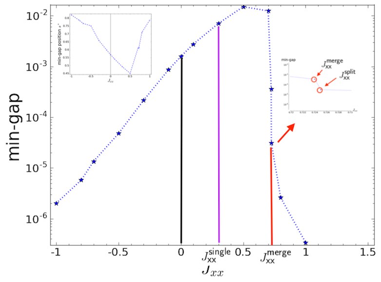
(b)

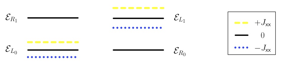
Figure 11: (a) Min-gap $\Delta$ vs $\mathsf{XX}$-coupler strength $J_{\mathsf{xx}}$ of ${\mathcal{H}}^{\mathsf{XX\!-\!Sys}}(J_{\mathsf{xx}},G_{\mathsf{driver}},G)$ for the weighted graph $G$ in Figure 5(a). $J^{\mathsf{merge}}_{\mathsf{xx}}\approx 0.724,J^{\mathsf{split}}_{\mathsf{xx}}\approx 0.725$. $J^{\mathsf{single}}_{\mathsf{xx}}\approx 0.3$. For $J_{\mathsf{xx}}\in(0,J^{\mathsf{single}}_{\mathsf{xx}}]$, $\Delta(J_{\mathsf{xx}})>\Delta(0)>\Delta(-J_{\mathsf{xx}})$ (“de-signed” is smaller); for $J_{\mathsf{xx}}>J^{\mathsf{merge}}_{\mathsf{xx}}$, $\Delta(J_{\mathsf{xx}})<\Delta(-J_{\mathsf{xx}})$ (“de-signed” is greater), but they are actually asymptotically the same. In this example, for $J_{\mathsf{xx}}\in(J^{\mathsf{single}}_{\mathsf{xx}},J^{\mathsf{merge}}_{\mathsf{xx}}]$, $\Delta(J_{\mathsf{xx}})>\Delta(-J_{\mathsf{xx}})$ (“de-signed” is smaller) but this is in general unknown as we do not know how small is the non-AC gap near $J^{\mathsf{merge}}_{\mathsf{xx}}$. For $J_{\mathsf{xx}}\in(0.3,0.5]$, the min-gap is a weak-AC gap which is not necessarily large (in the problem size). (b) For a small $J_{\mathsf{xx}}$, ${\mathcal{E}}_{L_{0}}(-J_{\mathsf{xx}})<{\mathcal{E}}_{L_{0}}(0)<{\mathcal{E}}_{L_{0}}(+J_{\mathsf{xx}})$ and ${\mathcal{E}}_{L_{1}}(-J_{\mathsf{xx}})<{\mathcal{E}}_{L_{1}}(0)<{\mathcal{E}}_{L_{1}}(+J_{\mathsf{xx}})$; while ${\mathcal{E}}_{R_{0}}$ and ${\mathcal{E}}_{R_{1}}$ stay the same because the $\mathsf{XX}$-couplers in the driver graph affect $L$ only. Also, ${\mathcal{E}}_{L_{1}}(-J_{\mathsf{xx}})-{\mathcal{E}}_{L_{0}}(-J_{\mathsf{xx}})={\mathcal{E}}_{L_{1}}(+J_{\mathsf{xx}})-{\mathcal{E}}_{L_{0}}(+J_{\mathsf{xx}})$ (c.f. Figure 1 in [18]). Both the anti-crossing point $s_{\mbox{\!\tiny$\times$}}$ and the width $\delta$ get shifted, result in either strengthened-AC ($-J_{\mathsf{xx}}$) or weakened-AC ($+J_{\mathsf{xx}}$) and ${\mathsf{AC\!\!-\!\!Gap}}(-J_{\mathsf{xx}})<{\mathsf{AC\!\!-\!\!Gap}}(0)<{\mathsf{AC\!\!-\!\!Gap}}(+J_{\mathsf{xx}})$.

We justify our Claim by three main observations below, supported by the numerical results of a scalable example. We leave a rigorous proof as future work. Nevertheless, our results already reveal the significance of the driver graph played in the non-stoquastic QA, and the essential difference of the ${\bf{EStoq}}{}$ and ${\bf{PNStoq}}{}$ due to different strength of $J_{\mathsf{xx}}$. The evolutions of ${\bf{EStoq}}{}$ QA and ${\bf{PNStoq}}{}$ QA can be very different. It is essential to distinguish them when considering non-stoquastic Hamiltonians. For example, our result in (I), where the non-stoquastic is ${\bf{EStoq}}{}$, already provides a counter-example to [18], as shown in Figure 11(a) (and in Figure 13 for the graph $G^{\prime}$ in the Appendix). In fact, it is more of a counter-argument, illustrated in Figure 11(b), to the intuition of Figure 1 in [18].

For simplicity, since $G_{\mathsf{driver}},G$ are fixed, we shall refer the system Hamiltonian by ${\mathcal{H}}^{\mathsf{XX\!-\!Sys}}(J_{\mathsf{xx}})$ for each $J_{\mathsf{xx}}$. Let ${\mathcal{E}}_{A_{i}}(J_{\mathsf{xx}},s^{*})\stackrel{{\scriptstyle\mathrm{def}}}{{=}}{\langle{{\mathcal{H}}^{\mathsf{XX\!-\!Sys}}(J_{\mathsf{xx}})(s^{*})}\rangle}_{A_{i},s^{*}}=\langle A_{i}(s^{*})|{\mathcal{H}}^{\mathsf{XX\!-\!Sys}}(J_{\mathsf{xx}})(s^{*})|A_{i}(s^{*})\rangle$ when (the eigenstate of ${\mathcal{H}}^{\mathsf{XX\!-\!Sys}}(J_{\mathsf{xx}})(s^{*})$) $|E_{i}(s^{*})\rangle\simeq|A_{i}(s^{*})\rangle$ for $i\in\{0,1\}$, $A\in\{L,R\},s^{*}\in\{s_{\mbox{\!\tiny$\times$}}^{-},s_{\mbox{\!\tiny$\times$}}^{+}\}$. We will consider the changes of the four energy values ${\mathcal{E}}_{L_{0}}(J_{\mathsf{xx}},s_{\mbox{\!\tiny$\times$}}^{-})$, ${\mathcal{E}}_{L_{1}}(J_{\mathsf{xx}},s_{\mbox{\!\tiny$\times$}}^{+})$, ${\mathcal{E}}_{R_{1}}(J_{\mathsf{xx}},s_{\mbox{\!\tiny$\times$}}^{-})$, ${\mathcal{E}}_{R_{0}}(J_{\mathsf{xx}},s_{\mbox{\!\tiny$\times$}}^{+})$ around the anti-crossing as $J_{\mathsf{xx}}$ changes. Since ${\mathcal{H}}^{\mathsf{XX\!-\!Sys}}(0)={\mathcal{H}}^{\mathsf{TFIM}}$ is stoquastic, by continuity, there exists a $J^{\mathsf{single}}_{\mathsf{xx}}>0$ such that ${\mathcal{H}}^{\mathsf{XX\!-\!Sys}}(J_{\mathsf{xx}})$ is eventually stoquastic, for $J_{\mathsf{xx}}\in(0,J^{\mathsf{single}}_{\mathsf{xx}}]$. Thus for, $J_{\mathsf{xx}}\in[-J^{\mathsf{single}}_{\mathsf{xx}},J^{\mathsf{single}}_{\mathsf{xx}}]$, the ground state coefficients $c_{i}(s)\geq 0$ for all $i$ and all $s\in[0,1]$.

Observation 1.

For sufficiently small $J_{\mathsf{xx}}>0$, ${\mathcal{H}}^{\mathsf{XX\!-\!Sys}}(J_{\mathsf{xx}})$ can be seen as a perturbed Hamiltonian from ${\mathcal{H}}^{\mathsf{XX\!-\!Sys}}(0)$, where the perturbation $V=(1-s)s\sum_{ij\in G_{\mathsf{driver}}}\sigma_{i}^{x}\sigma_{j}^{x}$. That is, ${\mathcal{H}}^{\mathsf{XX\!-\!Sys}}(J_{\mathsf{xx}})={\mathcal{H}}^{\mathsf{XX\!-\!Sys}}(0)+J_{\mathsf{xx}}V$. The entire evolution of ${\mathcal{H}}^{\mathsf{XX\!-\!Sys}}(J_{\mathsf{xx}})$ is a perturbed evolution of ${\mathcal{H}}^{\mathsf{XX\!-\!Sys}}(0)$. In particular, the ${(L,R)\!\!-\!\!{\footnotesize\textsc{Anti-crossing}}}$ of ${\mathcal{H}}^{\mathsf{XX\!-\!Sys}}(0)$ at $s_{\mbox{\!\tiny$\times$}}$ also evolves.

Observe that ${\langle{V}\rangle}_{L_{0},s}=\sum_{i\oplus j\in{\mathsf{E}}(G_{\mathsf{driver}})}c_{i}(s)c_{j}(s)>0$ because $c_{i}(s)>0,c_{j}(s)>0$ and ${\langle{V}\rangle}_{L_{1},s}=\sum_{i\oplus j\in{\mathsf{E}}(G_{\mathsf{driver}})}d_{i}(s)d_{j}(s)>0$ because $\mathsf{sgn}(d_{i}(s)d_{j}(s))=\mathsf{sgn}(c_{i}(s)c_{j}(s))>0$; while ${\langle{V}\rangle}_{R_{i},s}=0$ because there are no XX-couplers within $R$. For $J_{\mathsf{xx}}>0$, ${\mathcal{E}}_{L_{0}}(J_{\mathsf{xx}},s_{\mbox{\!\tiny$\times$}}^{-})>{\mathcal{E}}_{L_{0}}(0,s_{\mbox{\!\tiny$\times$}}^{-}),{\mathcal{E}}_{L_{1}}(J_{\mathsf{xx}},s_{\mbox{\!\tiny$\times$}}^{+})>{\mathcal{E}}_{L_{1}}(0,s_{\mbox{\!\tiny$\times$}}^{+})$ while ${\mathcal{E}}_{R_{0}}(J_{\mathsf{xx}},s_{\mbox{\!\tiny$\times$}}^{+})\approx{\mathcal{E}}_{R_{0}}(0,s_{\mbox{\!\tiny$\times$}}^{+}),{\mathcal{E}}_{R_{1}}(J_{\mathsf{xx}},s_{\mbox{\!\tiny$\times$}}^{-})\approx{\mathcal{E}}_{R_{1}}(0,s_{\mbox{\!\tiny$\times$}}^{-})$. This results in a weaker ${(L,R)\!\!-\!\!{\footnotesize\textsc{Anti-crossing}}}$ at $s_{\mbox{\!\tiny$\times$}}^{\prime}<s_{\mbox{\!\tiny$\times$}}$ with a larger $\delta^{\prime}>\delta$.

Since

$$\begin{cases}{\langle{H_{X}}\rangle}_{|E_{0}(s_{\mbox{\!\tiny$\times$}}^{-})\rangle}\approx{\langle{H_{X}}\rangle}_{L_{0},s_{\mbox{\!\tiny$\times$}}^{-}}\stackrel{{\scriptstyle\mathrm{def}}}{{=}}-2\sum_{l\in L}\sum_{k\in{\mathsf{nbr}}_{H_{X}}(l)}c_{l}(s_{\mbox{\!\tiny$\times$}}^{-})c_{k}(s_{\mbox{\!\tiny$\times$}}^{-})\\ {\langle{H_{{\mathsf{XX}}}}\rangle}_{|E_{0}(s_{\mbox{\!\tiny$\times$}}^{-})\rangle}\approx{\langle{H_{{\mathsf{XX}}}}\rangle}_{L_{0},s_{\mbox{\!\tiny$\times$}}^{-}}\stackrel{{\scriptstyle\mathrm{def}}}{{=}}2J_{\mathsf{xx}}\sum_{l\in L}\sum_{k\in{\mathsf{nbr}}_{H_{\mathsf{XX}}}(l)}c_{l}(s_{\mbox{\!\tiny$\times$}}^{-})c_{k}(s_{\mbox{\!\tiny$\times$}}^{-}),\\ \end{cases}$$

we have ${\langle{H_{X}}\rangle}_{|E_{0}(s_{\mbox{\!\tiny$\times$}}^{-})\rangle}<0$ and ${\langle{H_{{\mathsf{XX}}}}\rangle}_{|E_{0}(s_{\mbox{\!\tiny$\times$}}^{-})\rangle}$ is of the same sign of $J_{\mathsf{xx}}$. ${\langle{H_{D}}\rangle}_{|E_{1}(s_{\mbox{\!\tiny$\times$}}^{-})\rangle}={\langle{H_{X}}\rangle}_{|E_{1}(s_{\mbox{\!\tiny$\times$}}^{-})\rangle}$ as they are no $\mathsf{XX}$-couplers within R. Thus, as $J_{\mathsf{xx}}>0$ increases, the denominators in Eq. (10), ${\langle{\delta H}\rangle}_{|E_{0}(s_{\mbox{\!\tiny$\times$}}^{-})\rangle}-{\langle{\delta H}\rangle}_{|E_{1}(s_{\mbox{\!\tiny$\times$}}^{-})\rangle}$ and ${\langle{\delta H}\rangle}_{|E_{1}(s_{\mbox{\!\tiny$\times$}}^{+})\rangle}-{\langle{\delta H}\rangle}_{|E_{0}(s_{\mbox{\!\tiny$\times$}}^{+})\rangle}$, decrease, while the numerator in Eq. (10), $\delta$, increases, we have ${\mathsf{AC\!\!-\!\!Gap}}(J_{\mathsf{xx}})>{\mathsf{AC\!\!-\!\!Gap}}(0)$ by Corollary 2.4.

Conversely, $-J_{\mathsf{xx}}<0$, ${\mathcal{E}}_{L_{0}}(-J_{\mathsf{xx}},s_{\mbox{\!\tiny$\times$}}^{-})<{\mathcal{E}}_{L_{0}}(0,s_{\mbox{\!\tiny$\times$}}^{-}),{\mathcal{E}}_{L_{1}}(-J_{\mathsf{xx}},s_{\mbox{\!\tiny$\times$}}^{+})<{\mathcal{E}}_{L_{1}}(0,s_{\mbox{\!\tiny$\times$}}^{+})$, and it results in a stronger ${(L,R)\!\!-\!\!{\footnotesize\textsc{Anti-crossing}}}$ at $s_{\mbox{\!\tiny$\times$}}^{\prime\prime}>s_{\mbox{\!\tiny$\times$}}$ with a smaller $\delta^{\prime\prime}<\delta$ such that ${\mathsf{AC\!\!-\!\!Gap}}(0)>{\mathsf{AC\!\!-\!\!Gap}}(-J_{\mathsf{xx}})$. That is, we have ${\mathsf{AC\!\!-\!\!Gap}}(-J_{\mathsf{xx}})<{\mathsf{AC\!\!-\!\!Gap}}(0)<{\mathsf{AC\!\!-\!\!Gap}}(+J_{\mathsf{xx}})$. See Figure 9 for an example. By continuity, for $J_{\mathsf{xx}}\in[-J^{\mathsf{single}}_{\mathsf{xx}},J^{\mathsf{single}}_{\mathsf{xx}}]$, ${\mathsf{AC\!\!-\!\!Gap}}(J_{\mathsf{xx}})$ increases as $J_{\mathsf{xx}}$ increases. See Figure 11 of a plot of ${\mathsf{AC\!\!-\!\!Gap}}{}$ vs $J_{\mathsf{xx}}$ for ${\mathcal{H}}^{\mathsf{XX\!-\!Sys}}(J_{\mathsf{xx}},G_{\mathsf{driver}},G)$.

Observation 2.

If there is a $J_{\mathsf{xx}}$ such that $L$ is an arm of an anti-crossing in PNStoq ${\mathcal{H}}^{\mathsf{XX\!-\!Sys}}(G,J_{\mathsf{xx}},G_{\mathsf{driver}})$, then $L$ will be split into $L^{+}$ and $L^{-}$, with the coefficients for states in $L^{+}$ ($L^{-}$ resp.) being positive (negative resp.). When $|E_{0}(s)\rangle\simeq|L_{0}(s)\rangle$, the ground state energy

$$E_{0}(s)\approx(1-s)sJ_{\mathsf{xx}}\sum_{k\oplus k^{\prime}\in{\mathsf{E}}(G_{\mathsf{driver}})}c_{k}(s)c_{k^{\prime}}(s)+\sum_{k\in L^{+}\cup L^{-}}|c_{k}(s)|^{2}E_{k}.$$ (11)

Since $J_{\mathsf{xx}}>0$, the minimum of the (ground state) energy is attained when $L$ is split into $L^{+}$ and $L^{-}$ such that $c_{k}(s)c_{k^{\prime}}(s)<0$ for ${k\in L^{+},k^{\prime}\in L^{-}}$, and $\sum_{k\oplus k^{\prime}\in{\mathsf{E}}(G_{\mathsf{driver}})}c_{k}(s)c_{k^{\prime}}(s)$ is minimized. See Figure 8 for an illustration.

Furthermore, if we assume that $t_{i}\leq 2$, $L$ can be split into $L^{+}$ and $L^{-}$ such that the only $\mathsf{XX}$-neighboring is between one state in $L^{+}$ and another state in $L^{-}$. That is, there is no $\mathsf{XX}$-neighboring between states within $L^{+}$ or states within $L^{-}$. By $\mathsf{XX}$-neighboring we mean that there is exactly one XX-coupler between the two states. Since $|E_{1}(s)\rangle\approx|R_{1}(s)\rangle$ for $s\in[s_{1}(J_{\mathsf{xx}}),s_{2}(J_{\mathsf{xx}})]$, there can not have an anti-crossing between the first level and the second level during this interval. However, this does not immediately imply that the second-level gap is large, which is required in order to apply DQA-GS successfully. The second-level gap can still be small if the second-level energy $E_{2}(s)$ is close to $E_{1}(s)$ for $s\in[s_{1},s_{2}]$. However, it is likely that the second level energy $E_{2}(s)$ will be different for different $J_{\mathsf{xx}}$ while the first level energy $E_{1}(s)$ is independent with $J_{\mathsf{xx}}$. Therefore, there is a $J_{\mathsf{xx}}\in(J^{\mathsf{merge}}_{\mathsf{xx}},J^{\mathsf{double}}_{\mathsf{xx}}]$ such that the second-level gap is large.

Observation 3.

There exist $J^{\mathsf{split}}_{\mathsf{xx}}>0$ and $s_{c}$ such that ${\mathcal{H}}^{\mathsf{XX\!-\!Sys}}(J^{\mathsf{split}}_{\mathsf{xx}})$ has two anti-crossings bridged by $(L^{+},L^{-})$, namely, a ${(R,L)\!\!-\!\!{\footnotesize\textsc{Anti-crossing}}}$ at $s_{1}=s_{c}-\varepsilon$ and an ${(L,R)\!\!-\!\!{\footnotesize\textsc{Anti-crossing}}}$ at $s_{2}=s_{c}+\varepsilon$ for some $\varepsilon>0$. The necessary conditions (in Eq. (9)) for both ACs are satisfied. By the condition that ${\mathcal{E}}_{L_{0}}(J^{\mathsf{split}}_{\mathsf{xx}},s_{c})\approx{\mathcal{E}}_{R_{0}}(J^{\mathsf{split}}_{\mathsf{xx}},s_{c})\approx{\mathcal{E}}_{R_{0}}(0,s_{\mbox{\!\tiny$\times$}})$ and $s_{c}\approx s_{\mbox{\!\tiny$\times$}}$, we obtain $J^{\mathsf{split}}_{\mathsf{xx}}\approx\mu(\overline{E_{L}}-\overline{E_{R}})$ for some $\mu>0$, where $\overline{E_{L}}$ and $\overline{E_{R}}$ are the average energy (w.r.t problem Hamiltonian) in $L$ and $R$. As $J^{\mathsf{split}}_{\mathsf{xx}}$ decreases, there is a sharp exchange between the ground and first excited states and the two anti-crossings are merged, resulting in no AC at $J^{\mathsf{merge}}_{\mathsf{xx}}=J^{\mathsf{split}}_{\mathsf{xx}}-\epsilon$. See Figure 10 for an illustration. As $J_{\mathsf{xx}}$ increases from $J^{\mathsf{split}}_{\mathsf{xx}}$, the bridge length $2\varepsilon$ increases, the first AC weakens slightly, while the second AC strengthens slightly. There exists a $J^{\mathsf{double}}_{\mathsf{xx}}>J^{\mathsf{split}}_{\mathsf{xx}}$, such that when $J_{\mathsf{xx}}>J^{\mathsf{double}}_{\mathsf{xx}}$, the fist AC is too weak to be qualified as an anti-crossing.

$L$ and $R$ share some common vertices.

In our example, for illustrative purpose, $L$ and $R$ are not only disjoint subsets of $2^{[N]}$, but they are also disjoint in the ground set ($[N]$). However, this is not a required condition, as shown in $G^{\prime}$ in Figure 5(b) where the vertex $9$ appears both in some local minima and the global minimum. This is an important feature for otherwise the problem would be solved efficiently classically by solving $G\setminus L$.

Nested double-ACs or a double multi-level AC.

When there is a $t_{i}>2$, we take all the edges in the independent-cliques as the driver graph. However, in this case, there may be an AC between the first excited state and higher and we no longer can guarantee the large second-level gap. Instead, it may have a sequence of nested double-ACs (as shown in Figure 6(f)) or a double multi-level anti-crossing where the lowest excited states form a narrow band, as shown in Figure 14(a) in the Appendix for the 15-qubit instance in [10]. In this case, the system would undergo diabatic transitions to the higher excited states through a sequence of the first ACs of the nested double-ACs (or through the first AC of a double multi-level AC), and then returns to the ground state through the sequence of second ACs of the nested double-ACs (or through the second AC of a double multi-level AC). More details of the relationship between the driver graph structure and the nested double-ACs (or double multi-level ACs ) will be reported in our subsequent work.

Rules for constructing the driver graph.

In our above Claim, the driver graph $G_{\mathsf{driver}}$ is taken to be $G|_{L}$. Our arguments for the Observations actually reveal the intuition for constructing the driver graph. Namely, the idea is to include the $\mathsf{XX}$-couplers between local minima in $L$ (so to cause the split) and avoid including $\mathsf{XX}$-couplers that are coupling states in $R$ and its neighbors (so as not to weaken ${\mathcal{E}}_{R_{0}}$). We impose the independent-cliques structure in the local minima for the reason of justification, and also for the efficacy of identifying $G|_{L}$ with partial information of $L$, to be elaborated in the next section. We note that it is possible to relax the independent-cliques condition to almost-independent-cliques by allowing some edges between these cliques.

2.2.3 A General Procedure without Prior Knowledge of the Problem Structure

A natural question is: without knowing the problem structure, can one design an appropriate driver graph efficiently? As we note above, for the special GIC instances that we are considering, knowing the set $L$ (without any knowledge of $R$) will be sufficient to construct the appropriate driver graph. The idea follows that if we can identify some elements in $L$ (which is possible because these are the “wrong answers” from TFQA), it is possible to recover $G|_{L}$ explicitly and $L$ implicitly (as $L$ may consist of exponentially many maximal independent sets) by exploring the graph locally with a classical procedure, because of the special independent-cliques structure. More specifically, since we assume that the instance has an ${(L,R)\!\!-\!\!{\footnotesize\textsc{Anti-crossing}}}$ when running with TFQA algorithm, and if we further assume that the ${(L,R)\!\!-\!\!{\footnotesize\textsc{Anti-crossing}}}$ is the only super-polynomially small-gap in the system Hamiltonian, then with polynomial time, either by a stoquastic quantum annealer, or the simulated quantum annealing (SQA) [29, 30] , one can identify at least one local minimum $l_{0}$ in $L$, or a subset of local minima $P\subseteq L$ by repeating the procedure a polynomial number of times. This is (Step 1.1) of the Dic-Dac-Doa algorithm as described in Table 1.

Next, we identify an IC through $P$ (Step 1.2) as follows. First, based on the induced subgraph from the vertices in $P$, we identify a set of partial cliques of partites. (With some extra work, it is possible to screen out noisy local minima that are in $P$ but do not belong to the IC.) Then we greedily extend the partial cliques to include more vertices whose weights are similar to the weight of the partites. That is, we include the similar-weight vertices which are adjacent to the existing partites in the partial clique, and they are independent from other partites. Then we eliminate the vertices in the cliques found that are adjacent to some vertices in another clique to make sure the cliques are independent. This way we obtain a set of independent cliques of partites, IC, that generates a set of local minima $L$ containing $P$. The above procedure can be implemented in polynomial time. If $G|_{L}$ has a “clear cut boundary” (i.e. no ambiguous vertex which connects two cliques), we have $G[\mbox{IC}]=G|_{L}$. For example, the IC so discovered through a seed $l_{0}=\{1,3,6\}$ in Figure 5(b) will be the same as $G^{\prime}|_{L}$. However, the IC may not be unambiguous. Many different ICs are possible. Different procedures (e.g. with different vertex-weight allowances; or different vertex selection criteria) may be used to obtain different potential ICs.

To estimate a range of $J_{\mathsf{xx}}$ as in (Step 2.1), we first obtain an upper bound for the MWIS (corresponds to $-\overline{E^{R}}$). Such a good upper bound can be obtained through a weighted clique cover as used in the branch-and-bound algorithm for MWIS [26, 27, 28]. Together with the estimate bound for $\overline{E_{L}}$, we obtain a possible range $(0,U]$ for $J_{\mathsf{xx}}$. We then in (Step 2.2) run the QA a polynomial number of different $J_{\mathsf{xx}}$ evenly distributed in the range$(0,U]$, by annealing ${\mathcal{H}}^{\mathsf{XX\!-\!Sys}}(J_{\mathsf{xx}},G_{\mathsf{driver}},G)$ in polynomial time and record the best answer.

Quantum Speedup.

If the instance has the independent-cliques structure such that $G[\mbox{IC}]=G|_{L}$, and there is a $J_{\mathsf{xx}}\in(0,U]$ such that there is a double-AC in ${\mathcal{H}}^{\mathsf{XX\!-\!Sys}}(J_{\mathsf{xx}},G_{\mathsf{driver}},G)$ as described in Claim (II), the above algorithm Dic-Dac-Doa will successfully find the ground state through DQA-GS in polynomial time, with an $O(c^{\alpha})$ speedup over the ${(L,R)\!\!-\!\!{\footnotesize\textsc{Anti-crossing}}}$ plagued stoquastic algorithm where $\alpha={\mathsf{dist}}_{H_{D}}(L,R)$. It may have similar speedup for some other classical heuristics that developed in comparison with QA algorithms (see e.g. [30]). While Claim (II) remains to be more rigorously proved, it is worthwhile to point out that the mechanism of achieving speedup here is through a bridged double-AC which requires the necessity of +${\mathsf{XX}}$-interactions, so as to overcome the single-AC in the stoquastic case. At the same time, this is achieved through a “cancellation” effect, and not by removing the local minima from the graph as in the classical algorithm. This point perhaps would gain much appreciation when comparing with the classical branch-and-bound solver for the MWIS where a clique cover is pruned. From our perspective, this mechanism of achieving the speedup (by overcoming the local minima) does not seem to have a similar classical counterpart, c.f. [8].

Remark.

For $J_{\mathsf{xx}}\in(J^{\mathsf{single}}_{\mathsf{xx}},J^{\mathsf{merge}}_{\mathsf{xx}})$, there is no AC in ${\mathcal{H}}^{\mathsf{XX\!-\!Sys}}(J_{\mathsf{xx}},G_{\mathsf{driver}},G)$. However, the min-gap may still be exponentially small. If the min-gap is polynomially large, Dic-Dac-Doa would also successfully solve the problem adiabatically in polynomial time. It will be important to investigate the question whether for this range of $J_{\mathsf{xx}}$, the non-stoquastic but eventually stoquastic ${\mathcal{H}}^{\mathsf{XX\!-\!Sys}}(J_{\mathsf{xx}},G_{\mathsf{driver}},G)$ is VGP or if it can be efficiently simulated by QMC algorithms.

3 Discussion

In this paper, we point out the essential distinction of eventually stoquastic (EStoq) and proper-non-stoquastic (PNStoq) for the non-stoquastic Hamiltonians from the algorithmic perspective. The quantum evolutions of the EStoq QA and PNStoq QA can be very different, especially when comparing their spectral gaps with their de-signed counterparts. Furthermore, we demonstrate the essentiality of the design of the $\mathsf{XX}$-driver graph (which specifies which $\mathsf{XX}$-couplers to be included) that has not been considered by other previous work.

In particular, we describe a proper-non-stoquastic QA algorithm that can overcome the anti-crossing presented in the transeverse-field QA algorithm and achieve a quantum speedup for quantum optimization through DQA-GS, with the two essential ingredients: non-stoquastic +$\mathsf{XX}$-couplers and the structure of the $\mathsf{XX}$-driver graph. This is in contrast to the recent comments made in [5] that the “non-stoquasticity is desirable but not essential for quantum enhancement”, where neither the distinction of non-stoquasticity nor the structure of driver graph is taken into consideration. The essentiality of the PNStoq +$\mathsf{XX}$-couplers comes from the ability to overcome the inevitable single-AC small gap in the TFQA by “splitting” the AC into two bridged ACs (a double-AC) that would then enable DQA-GS to solve the problem efficiently. The possibility of constructing the desired driver graph efficiently is because one can make use of the “wrong answers” from the anti-crossing plagued TFQA, together with the imposed special independent-cliques condition. The quantum speedup through the idea of double-AC-enabled-DQA was first proposed in [6], where an oracular stoquastic QA algorithm for solving the glued-tree problem in polynomial time is presented. There the double-AC is formed by two identical anti-crossings (due to the symmetric evolution at the middle). In contrast, our double-AC is formed by two anti-symmetric anti-crossings that share a common arm of the opposite sign as the bridge. As we argue above, the proper-non-stoquastic interactions (which cause the negative amplitudes in the ground state) are essential in our argument to form the bridge. Admittedly, our algorithmic procedure still requires a more rigorous proof, nevertheless, we believe that we have provided enough arguments and evidence that are confirmed by (scalable) numerical examples. In particular, when the hard instances whose local minima subgraph is indeed the same as the graph $G[\mbox{IC}]$ discovered by our algorithm Dic-Dac-Doa, then there would be a double-AC or a sequenced of nested double-ACs or a narrow band that enable DQA to solve the problem successfully in polynomial time. This would achieve an exponential speedup over the stoquastic algorithm, and possible exponential speedup over the state-of-the-art classical algorithms for such instances.

Furthermore, there are some reasons to further support our arguments: (1) We make use of the exclusive quantum feature (negative amplitudes) in our algorithm. (2) The special structure of the GIC instances are believed to one of the obstacles for the efficient classical algorithms (heuristics or exact solvers). (3) Proper-non-stoquastic (with $\mathsf{XX}$-driver) may not be VGP[16], and thus not QMC-simulable.

The insights of this work are obtained based on the novel characterizations of a modified and generalized parametrization definition of an anti-crossing in the context of QOA. We demonstrate how the parametrized AC can be used as a tool to open up the ‘black-box’ of the QOA algorithm, and thus facilitate the analysis and design of adiabatic or diabatic QA algorithms. In particular, we derive the necessary conditions for the formation of an anti-crossing. This provides us algorithmic insight into the relationship between an anti-crossing and the structure of the local and global minima of the problem. In our subsequent work, we study with what extra conditions, the necessary conditions are also sufficient.

There are several future works to be followed: (1) We are developing a framework to better understand the role of the negative amplitudes play in the non-stoquastic Hamiltonians. (2) We construct a scalable family of GIC instances that are believed to be hard for the classical algorithms and the TFQA algorithms. We will also address the question of practical applications of GIC instances, and the relaxation of the independent-cliques condition to the almost-independent-cliques such that some edges between cliques are allowed. (3) We will investigate how to best obtain a subset of local minima to build the $\mathsf{XX}$-driver graph. There are also several different ways to improve the design of the $\mathsf{XX}$-driver graph. (4) We can consider the possible generalization of the AC definition to include a multi-level anti-crossing such that the anti-crossing is between one energy level and a band of of closely tie together energy levels (a pseudo degenerate state) which can make the analysis of the algorithm more robust. (5) The problem of the intertwined sparse universal hardware graph and the minor-embedding problem [32, 33], including both problem graph and driver graph, will also be addressed.

Finally, since proper-non-stoquastic Hamiltonians can be simulated by other quantum models with polynomial overhead, it is our hope that our method provides a quantum algorithm design paradigm for solving the optimization problems.

4 Methods

4.1 Proof of Proposition 2.2

Proof.

The derivation is based on the assumption of the linear interpolation between $H_{D}$ (driver Hamiltonian) and $H_{P}$ (problem Hamiltonian). That is, $H(s)=(1-s)H_{D}+sH_{P}$. (The catalyst version will be approximated.) Note that we can write $H(s)=H(s_{\mbox{\!\tiny$\times$}})+(s-s_{\mbox{\!\tiny$\times$}})(H_{P}-H_{D})$. The idea is based on the non-degenerate perturbation theory where the unperturbed Hamiltonian $H^{(0)}=H(s_{\mbox{\!\tiny$\times$}})$, and the perturbation $\delta H(=\frac{\delta H}{\delta s})=H_{P}-H_{D}$. We apply the perturbation to $H(s_{\mbox{\!\tiny$\times$}}+\lambda)=H(s_{\mbox{\!\tiny$\times$}})+\lambda\delta H$, where $|\lambda|$ is sufficiently small. (The standard non-degenerate perturbation theory usually apply to the positive small $\lambda$. See e.g. [23]. Here we apply to both positive and negative $\lambda$. For the small negative $\lambda$, one can think of it as it equivalently applies the negative sign to $\delta H$.) From the perturbation theory (see, e.g. [23] Chapter 1 page 8), we have the states and energies for $H(s_{\mbox{\!\tiny$\times$}}+\lambda)=H(s_{\mbox{\!\tiny$\times$}})+\lambda\delta H$:

$$\begin{cases}|E_{n}(s_{\mbox{\!\tiny$\times$}}+\lambda)\rangle=|E_{n}(s_{\mbox{\!\tiny$\times$}})\rangle-\lambda\sum_{k\neq n}\frac{\delta H_{kn}(s_{\mbox{\!\tiny$\times$}})}{E_{k}(s_{\mbox{\!\tiny$\times$}})-E_{n}(s_{\mbox{\!\tiny$\times$}})}|E_{k}(s_{\mbox{\!\tiny$\times$}})\rangle+O(\lambda^{2})\\ E_{n}(s_{\mbox{\!\tiny$\times$}}+\lambda)=E_{n}(s_{\mbox{\!\tiny$\times$}})+\lambda\delta H_{nn}(s_{\mbox{\!\tiny$\times$}})-\lambda^{2}\sum_{k\neq n}\frac{|\delta H_{kn}(s_{\mbox{\!\tiny$\times$}})|^{2}}{E_{k}(s_{\mbox{\!\tiny$\times$}})-E_{n}(s_{\mbox{\!\tiny$\times$}})}+O(\lambda^{3})\end{cases}$$ (12)

where $\delta H_{mn}(s_{\mbox{\!\tiny$\times$}})\equiv\langle E_{m}(s_{\mbox{\!\tiny$\times$}})|\delta H|E_{n}(s_{\mbox{\!\tiny$\times$}})\rangle$. By definition (condition (a)), $\Delta_{10}(s_{\mbox{\!\tiny$\times$}})=E_{1}(s_{\mbox{\!\tiny$\times$}})-E_{0}(s_{\mbox{\!\tiny$\times$}})<<E_{2}(s_{\mbox{\!\tiny$\times$}})-E_{0}(s_{\mbox{\!\tiny$\times$}})=\Delta_{20}(s_{\mbox{\!\tiny$\times$}})$, and $|\lambda|$ is sufficiently small, we apply the above formulae to $n=0,1$ and obtain:

$$\begin{cases}|E_{0}(s_{\mbox{\!\tiny$\times$}}+\lambda)\rangle\simeq|E_{0}(s_{\mbox{\!\tiny$\times$}})\rangle-\lambda\frac{\delta H_{10}(s_{\mbox{\!\tiny$\times$}})}{\Delta_{10}(s_{\mbox{\!\tiny$\times$}})}|E_{1}(s_{\mbox{\!\tiny$\times$}})\rangle\\ |E_{1}(s_{\mbox{\!\tiny$\times$}}+\lambda)\rangle\simeq|E_{1}(s_{\mbox{\!\tiny$\times$}})\rangle+\lambda\frac{\delta H_{10}(s_{\mbox{\!\tiny$\times$}})}{\Delta_{10}(s_{\mbox{\!\tiny$\times$}})}|E_{0}(s_{\mbox{\!\tiny$\times$}})\rangle\\ \end{cases}$$ (13)

and

$$\begin{cases}E_{0}(s_{\mbox{\!\tiny$\times$}}+\lambda)\doteq E_{0}(s_{\mbox{\!\tiny$\times$}})+\lambda\delta H_{00}(s_{\mbox{\!\tiny$\times$}})-\lambda^{2}\frac{|\delta H_{10}(s_{\mbox{\!\tiny$\times$}})|^{2}}{\Delta_{10}(s_{\mbox{\!\tiny$\times$}})}\\ E_{1}(s_{\mbox{\!\tiny$\times$}}+\lambda)\doteq E_{1}(s_{\mbox{\!\tiny$\times$}})+\lambda\delta H_{11}(s_{\mbox{\!\tiny$\times$}})+\lambda^{2}\frac{|\delta H_{10}(s_{\mbox{\!\tiny$\times$}})|^{2}}{\Delta_{10}(s_{\mbox{\!\tiny$\times$}})}\end{cases}$$ (14)

[where the error tolerance in $\doteq$ due to perturbation is $\epsilon_{p}<<\Delta_{10}(s_{\mbox{\!\tiny$\times$}})/\Delta_{20}(s_{\mbox{\!\tiny$\times$}}))$.] Eq.(14) thus gives rise to the two parabolas with $\beta_{0}=\delta H_{00}(s_{\mbox{\!\tiny$\times$}})$ and $\beta_{1}=\delta H_{11}(s_{\mbox{\!\tiny$\times$}})$ and $\alpha=\frac{|\delta H_{10}(s_{\mbox{\!\tiny$\times$}})|^{2}}{\Delta_{10}(s_{\mbox{\!\tiny$\times$}})}>0$. Furthermore, $\beta_{0}\simeq\beta_{1}$ (by Property (C4)). This proves Property (C1).

From Eq. (18), for all $k\in\widetilde{L}\cup\widetilde{R}$, we have

$$\begin{cases}c_{k}(s_{\mbox{\!\tiny$\times$}}+\lambda)\doteq c_{k}(s_{\mbox{\!\tiny$\times$}})-\lambda\frac{\delta H_{10}(s_{\mbox{\!\tiny$\times$}})}{\Delta_{10}(s_{\mbox{\!\tiny$\times$}})}d_{k}(s_{\mbox{\!\tiny$\times$}})\\ d_{k}(s_{\mbox{\!\tiny$\times$}}+\lambda)\doteq d_{k}(s_{\mbox{\!\tiny$\times$}})+\lambda\frac{\delta H_{10}(s_{\mbox{\!\tiny$\times$}})}{\Delta_{10}(s_{\mbox{\!\tiny$\times$}})}c_{k}(s_{\mbox{\!\tiny$\times$}})\end{cases}$$ (15)

for $\lambda\in[-\delta,\delta]$ (the error tolerance in $\doteq$ is $\epsilon_{p}$).

From condition (iv), we have $|L_{0}(s-\delta)|\approx 1-\gamma$ while $|L_{0}(s+\delta)|\approx 0$, we have $|c_{l}(s)|\downarrow$; and $|L_{1}(s+\delta)|\approx 1-\gamma$ while $|L_{1}(s-\delta)|\approx 0$, we have $|d_{l}(s)|\uparrow$, for all $l\in L$. Similarly, we have $|c_{r}(s)|\uparrow,|d_{r}(s)|\downarrow$, for all $r\in R$. This proves Property (C2).

To show Property (C3), we distinct two possible cases: (1) $\delta H_{10}(s_{\mbox{\!\tiny$\times$}})>0$ and (2) $\delta H_{10}(s_{\mbox{\!\tiny$\times$}})<0$. Assume case (1), i.e. $\delta H_{10}(s_{\mbox{\!\tiny$\times$}})>0$. For $l\in L$, from the above arguments for Property (C2), we $|c_{l}(s)|\downarrow,|d_{r}(s)|\uparrow$, i.e. $|c_{l}(s)|$ is decreasing while $|d_{r}(s)|$ is increasing. By Eq. (15) , $c_{l}(s)$ must be in the same sign of $d_{l}(s)$ (i.e. $c_{l}(s)d_{l}(s)>0$) (otherwise both would be increasing, a contradiction.) Similarly, we can deduce that $c_{r}(s)d_{r}(s)<0\mbox{ for }r\in R$. That is, we have

$$\left\{\begin{array}[]{l}L_{0}\mbox{ and }L_{1}\mbox{ in the same sign: }\mathsf{sgn}(c_{l}(s))\mathsf{sgn}(d_{l}(s))=+1\mbox{ for all }l\in L\\ R_{0}\mbox{ and }R_{1}\mbox{ in the opposite sign: }\mathsf{sgn}(c_{r}(s))\mathsf{sgn}(d_{r}(s))=-1\mbox{ for all }r\in R\\ \end{array}\right.$$

where $s:s_{\mbox{\!\tiny$\times$}}-\delta\leadsto s_{\mbox{\!\tiny$\times$}}+\delta$.

Similarly, we can show that for case (2):

$$\left\{\begin{array}[]{l}L_{0}\mbox{ and }L_{1}\mbox{ in the opposite sign: }\mathsf{sgn}(c_{l}(s))\mathsf{sgn}(d_{l}(s))=-1\mbox{ for all }l\in L\\ R_{0}\mbox{ and }R_{1}\mbox{ in the same sign: }\mathsf{sgn}(c_{r}(s))\mathsf{sgn}(d_{r}(s))=+1\mbox{ for all }r\in R\\ \end{array}\right.$$

where $s:s_{\mbox{\!\tiny$\times$}}-\delta\leadsto s_{\mbox{\!\tiny$\times$}}+\delta$. This proves Property (C3).

To prove Property (C4), substitute $\lambda=-\delta,+\delta$ to Eq. (15), we get

$$\begin{cases}c_{k}(s_{\mbox{\!\tiny$\times$}}-\delta)\doteq c_{k}(s_{\mbox{\!\tiny$\times$}})+\delta\frac{\delta H_{10}(s_{\mbox{\!\tiny$\times$}})}{\Delta_{10}(s_{\mbox{\!\tiny$\times$}})}d_{k}(s_{\mbox{\!\tiny$\times$}})\\ c_{k}(s_{\mbox{\!\tiny$\times$}}+\delta)\doteq c_{k}(s_{\mbox{\!\tiny$\times$}})-\delta\frac{\delta H_{10}(s_{\mbox{\!\tiny$\times$}})}{\Delta_{10}(s_{\mbox{\!\tiny$\times$}})}d_{k}(s_{\mbox{\!\tiny$\times$}})\end{cases}$$

Summing up the above two equations, we get $2c_{k}(s_{\mbox{\!\tiny$\times$}})\doteq c_{k}(s_{\mbox{\!\tiny$\times$}}-\delta)+c_{k}(s_{\mbox{\!\tiny$\times$}}+\delta)$. Similarly, $2d_{k}(s_{\mbox{\!\tiny$\times$}})\doteq d_{k}(s_{\mbox{\!\tiny$\times$}}-\delta)+d_{k}(s_{\mbox{\!\tiny$\times$}}+\delta)$. By the full-exchange condition in Eq.(3), we have $|c_{k}(s_{\mbox{\!\tiny$\times$}}-\delta)|\doteq|d_{k}(s_{\mbox{\!\tiny$\times$}}+\delta)|$ and $|c_{k}(s_{\mbox{\!\tiny$\times$}}+\delta)|\doteq|d_{k}(s_{\mbox{\!\tiny$\times$}}-\delta)|$, consequently we have $|c_{k}(s_{\mbox{\!\tiny$\times$}})|\doteq|d_{k}(s_{\mbox{\!\tiny$\times$}})|$. This proves Property (C4). ∎

Remark on the proof.

This derivation is based on the linear interpolation path. However, for the catalyst, we can similarly apply the arguments to the linear approximation near the anti-crossing point, with $\delta H=H_{P}-s_{\mbox{\!\tiny$\times$}}H_{D}$.

4.2 Proof of the Necessary Conditions

As in the proof of the properties of the anti-crossing, we express the system Hamiltonian in a perturbed form (but we are not applying the perturbation theory here; our arguments are exact). For any $s_{0}\in[0,1]$, $0<\lambda(<1-s_{0})$,

$$H(s_{0}+\lambda)=H(s_{0})+\lambda\delta H$$ (16)

where $\delta H=H_{P}-H_{D}$. Let ${\langle{\delta{\mathcal{H}}}\rangle}_{|\Psi\rangle}\stackrel{{\scriptstyle\mathrm{def}}}{{=}}\langle\Psi|\delta{\mathcal{H}}|\Psi\rangle$.

Lemma 4.1.

For any two levels $i,j\geq 0$, $s_{0}\in[0,1]$, and $0<\lambda(<1-s_{0})$, we have

$$E_{i}(s_{0}+\lambda)-E_{j}(s_{0})=\lambda\frac{\langle E_{j}(s_{0})|\delta H|E_{i}(s_{0}+\lambda)\rangle}{\langle{E_{j}(s_{0})}|E_{i}(s_{0}+\lambda)\rangle}$$ (17)

Proof.

Since $H(s_{0}+\lambda)|E_{i}(s_{0}+\lambda)\rangle=E_{i}(s_{0}+\lambda)|E_{i}(s_{0}+\lambda)\rangle$, we have

$$(E_{i}(s_{0}+\lambda)-H(s_{0}))|E_{i}(s_{0}+\lambda)\rangle=\lambda\delta H|E_{i}(s_{0}+\lambda)\rangle$$ (18)

Apply $\langle E_{j}(s_{0})|$ to the left of the above equation, we get Eq. (4.3). ∎

Proof.

(of Theorem 2.3) We apply Lemma 4.1 to an ${(L,R)\!\!-\!\!{\footnotesize\textsc{Anti-crossing}}}$ at $s_{\mbox{\!\tiny$\times$}}$ with width $\delta$, by setting $\{i,j\}=\{0,1\}$, and $s_{0}=s_{\mbox{\!\tiny$\times$}}^{-},s_{0}+\lambda=s_{\mbox{\!\tiny$\times$}}^{+}$. That is, $\lambda=2\delta$. We get

$$\begin{cases}E_{1}(s_{\mbox{\!\tiny$\times$}}^{+})-E_{0}(s_{\mbox{\!\tiny$\times$}}^{-})=2\delta\frac{\langle E_{0}(s_{\mbox{\!\tiny$\times$}}^{-})|\delta H|E_{1}(s_{\mbox{\!\tiny$\times$}}^{+})\rangle}{\langle{E_{0}(s_{\mbox{\!\tiny$\times$}}^{-})}|E_{1}(s_{\mbox{\!\tiny$\times$}}^{+})\rangle}\\ E_{0}(s_{\mbox{\!\tiny$\times$}}^{+})-E_{1}(s_{\mbox{\!\tiny$\times$}}^{-})=2\delta\frac{\langle E_{1}(s_{\mbox{\!\tiny$\times$}}^{-})|\delta H|E_{0}(s_{\mbox{\!\tiny$\times$}}^{+})\rangle}{\langle{E_{1}(s_{\mbox{\!\tiny$\times$}}^{-})}|E_{0}(s_{\mbox{\!\tiny$\times$}}^{+})\rangle}\end{cases}$$

By the full-exchange condition in Eq. (4), we have

$$\begin{cases}|{\langle{E_{0}(s_{\mbox{\!\tiny$\times$}}^{-})}|E_{1}(s_{\mbox{\!\tiny$\times$}}^{+})\rangle}|\approx|{\langle{L_{0}(s_{\mbox{\!\tiny$\times$}}^{-})}|L_{1}(s_{\mbox{\!\tiny$\times$}}^{+})\rangle}|\approx 1\\ |{\langle{E_{1}(s_{\mbox{\!\tiny$\times$}}^{-})}|E_{0}(s_{\mbox{\!\tiny$\times$}}^{+})\rangle}|\approx|{\langle{R_{1}(s_{\mbox{\!\tiny$\times$}}^{-})}|R_{0}(s_{\mbox{\!\tiny$\times$}}^{+})\rangle}|\approx 1.\end{cases}$$ (19)

We thus have

$$\begin{cases}E_{1}(s_{\mbox{\!\tiny$\times$}}^{+})-E_{0}(s_{\mbox{\!\tiny$\times$}}^{-})\approx 2\delta{\langle{\delta H}\rangle}_{|E_{0}(s_{\mbox{\!\tiny$\times$}}^{-})\rangle}\\ E_{0}(s_{\mbox{\!\tiny$\times$}}^{+})-E_{1}(s_{\mbox{\!\tiny$\times$}}^{-})\approx 2\delta{\langle{\delta H}\rangle}_{|E_{1}(s_{\mbox{\!\tiny$\times$}}^{-})\rangle}\end{cases}$$ (20)

By Property (C1),

$$E_{1}(s_{\mbox{\!\tiny$\times$}}^{+})-E_{0}(s_{\mbox{\!\tiny$\times$}}^{+})=E_{1}(s_{\mbox{\!\tiny$\times$}}^{-})-E_{0}(s_{\mbox{\!\tiny$\times$}}^{-})\doteq 2\alpha\delta^{2}$$ (21)

where $\alpha=\frac{|\langle E_{1}(s_{\mbox{\!\tiny$\times$}})|\delta H|E_{0}(s_{\mbox{\!\tiny$\times$}})\rangle|^{2}}{\Delta_{10}(s_{\mbox{\!\tiny$\times$}})}>0$. Subtract the two equations in Eq.(20), we thus get

$$\begin{cases}{\langle{\delta H}\rangle}_{|E_{0}(s_{\mbox{\!\tiny$\times$}}^{-})\rangle}-{\langle{\delta H}\rangle}_{|E_{1}(s_{\mbox{\!\tiny$\times$}}^{-})\rangle}\approx 2\eta^{2}\frac{\delta}{\Delta_{01}(s_{\mbox{\!\tiny$\times$}})}\\ {\langle{\delta H}\rangle}_{|E_{1}(s_{\mbox{\!\tiny$\times$}}^{+})\rangle}-{\langle{\delta H}\rangle}_{|E_{0}(s_{\mbox{\!\tiny$\times$}}^{+})\rangle}\approx 2\eta^{2}\frac{\delta}{\Delta_{01}(s_{\mbox{\!\tiny$\times$}})}\end{cases}$$ (22)

where $\eta=\langle E_{1}(s_{\mbox{\!\tiny$\times$}})|\delta H|E_{0}(s_{\mbox{\!\tiny$\times$}})\rangle$.

In particular, we have

$$\begin{cases}{\langle{\delta H}\rangle}_{|E_{0}(s_{\mbox{\!\tiny$\times$}}^{-})\rangle}>{\langle{\delta H}\rangle}_{|E_{1}(s_{\mbox{\!\tiny$\times$}}^{-})\rangle}\\ {\langle{\delta H}\rangle}_{|E_{1}(s_{\mbox{\!\tiny$\times$}}^{+})\rangle}>{\langle{\delta H}\rangle}_{|E_{0}(s_{\mbox{\!\tiny$\times$}}^{+})\rangle}\end{cases}$$ (23)

∎

4.3 Proofs of AC-gap Bound

Lemma 4.2.

Assume $\alpha={\mathsf{dist}}_{H_{D}}(L,R)>3.$

$$\Delta_{10}(s_{\mbox{\!\tiny$\times$}})=\Theta\left(\left|\sum_{i\in g(L),j\in g(R),\langle i|H_{D}|j\rangle\neq 0}c_{i}(s_{\mbox{\!\tiny$\times$}})c_{j}(s_{\mbox{\!\tiny$\times$}})\langle i|H_{D}|j\rangle\right|\right)$$ (24)

where $g(L)=\{i\in n(L):\exists j\in n(R)\mbox{ s.t. }\langle i|H_{D}|j\rangle\neq 0\}$, $g(R)=\{j\in n(R):\exists i\in n(L)\mbox{ s.t. }\langle i|H_{D}|j\rangle\neq 0\}$.

Proof.

By definition, $E_{i}(s_{\mbox{\!\tiny$\times$}})=\langle E_{i}(s_{\mbox{\!\tiny$\times$}})|H(s_{\mbox{\!\tiny$\times$}})|E_{i}(s_{\mbox{\!\tiny$\times$}})\rangle$ for $i=0,1$. Thus, we have

$$\Delta_{10}(s_{\mbox{\!\tiny$\times$}})=\langle E_{1}(s_{\mbox{\!\tiny$\times$}})|H(s_{\mbox{\!\tiny$\times$}})|E_{1}(s_{\mbox{\!\tiny$\times$}})\rangle-\langle E_{0}(s_{\mbox{\!\tiny$\times$}})|H(s_{\mbox{\!\tiny$\times$}})|E_{0}(s_{\mbox{\!\tiny$\times$}})\rangle$$ (25)

We assume that the anti-crossing is $(1-\epsilon_{v})$-full-exchange and it satisfies the approximate SAS property in (C4).

First, we show that if the SAS is exact, i.e.,

$$(*)\begin{cases}|E_{0}(s_{\mbox{\!\tiny$\times$}})\rangle=|\widetilde{L}(s_{\mbox{\!\tiny$\times$}})\rangle{\color[rgb]{1,0,0}+}|\widetilde{R}(s_{\mbox{\!\tiny$\times$}})\rangle\\ |E_{1}(s_{\mbox{\!\tiny$\times$}})\rangle=|\widetilde{L}(s_{\mbox{\!\tiny$\times$}})\rangle{\color[rgb]{1,0,0}-}|\widetilde{R}(s_{\mbox{\!\tiny$\times$}})\rangle\end{cases}$$

the $\mathsf{AC\!\!-\!\!Gap}$ is contributed from the coefficients of negligible states. Substitute (*) into Eq. (25), because of the cancellation of the opposite terms, we have $\Delta_{10}(s_{\mbox{\!\tiny$\times$}})=-4\langle\widetilde{L}(s_{\mbox{\!\tiny$\times$}})|H(s_{\mbox{\!\tiny$\times$}})|\widetilde{R}(s_{\mbox{\!\tiny$\times$}})\rangle$. By assumption that $\widetilde{L}\cap\widetilde{R}=\emptyset$, we have $\langle\widetilde{L}(s_{\mbox{\!\tiny$\times$}})|H_{P}|\widetilde{R}(s_{\mbox{\!\tiny$\times$}})\rangle=0$. Thus, $\Delta_{10}(s_{\mbox{\!\tiny$\times$}})\doteq-4(1-s)\langle\widetilde{L}(s_{\mbox{\!\tiny$\times$}})|H_{D}|\widetilde{R}(s_{\mbox{\!\tiny$\times$}})\rangle.$ If ${\mathsf{dist}}_{H_{D}}(L,R)>3$, it implies $\langle L|H_{D}|R\rangle=0$, and thus we have $\Delta_{10}(s_{\mbox{\!\tiny$\times$}})\doteq-4(1-s)\langle n(L)(s_{\mbox{\!\tiny$\times$}})|H_{D}|n(R)(s_{\mbox{\!\tiny$\times$}})\rangle$.

Let $g(L)=\{i\in n(L):\exists j\in n(R)\mbox{ s.t. }\langle i|H_{D}|j\rangle\neq 0\}$, $g(R)=\{j\in n(R):\exists i\in n(L)\mbox{ s.t. }\langle i|H_{D}|j\rangle\neq 0\}$ be the set of states that contribute non-zero values to the gap.

That is,

$$\Delta_{10}(s_{\mbox{\!\tiny$\times$}})) =\kappa\langle g(L)(s_{\mbox{\!\tiny$\times$}})|H_{D}|g(R)(s_{\mbox{\!\tiny$\times$}})\rangle$$

$$=\kappa\sum_{i\in g(L),j\in g(R),\langle i|H_{D}|j\rangle\neq 0}c_{i}(s_{\mbox{\!\tiny$\times$}})c_{j}(s_{\mbox{\!\tiny$\times$}})\langle i|H_{D}|j\rangle$$

$$=\kappa\sum_{i\in g(L),j\in g(R),\langle i|H_{D}|j\rangle\neq 0}d_{i}(s_{\mbox{\!\tiny$\times$}})d_{j}(s_{\mbox{\!\tiny$\times$}})\langle i|H_{D}|j\rangle$$

where $\kappa=-4(1-s)$.

When the AC is $(1-\epsilon_{v})$-full-exchange, the small error due to the differences in $c,d$ of the non-negligible states is absorbed by the above term. ∎

Remark.

As the AC becomes weaker, the error term due to the difference in $c,d$ of the non-negligible states can be large enough to dominate the gap size, in this case the min-gap will be $\omega(\zeta^{\alpha})$ (strictly greater than the order of $\zeta^{\alpha}$).

The above lemma implies that the non-zero contributions to the gap come from the (at least $(\alpha/2)!$ ) states in $g(L)$ and $g(R)$ from the ground state . Notice that we express the $\mathsf{AC\!\!-\!\!Gap}$ only on the ground state (it can be also on the first excited state as $c_{k}(s_{\mbox{\!\tiny$\times$}})\doteq d_{k}(s_{\mbox{\!\tiny$\times$}})$ ) instead of the difference between the two levels.

Next we show that the coefficients $c_{k}$ decrease in geometric order of its distance from $L,R$, and thus the dominated terms are those in the path of the shortest distance between $L,R$.

Proof.

(of Theorem 2.5) First, assume the anti-crossing is near the end of annealing (i.e. $s_{\mbox{\!\tiny$\times$}}\approx 1$) (with $R$ as the ground state, and $L$ as the first excited state) as in the perturbative crossing case.

Observe that: For $k\in n(R)$: $c_{k}(s_{\mbox{\!\tiny$\times$}}-\delta)\neq 0\longrightarrow c_{k}(s_{\mbox{\!\tiny$\times$}}+\delta)=0$, we have $c_{k}(s_{\mbox{\!\tiny$\times$}})\doteq 1/2c_{k}(s_{\mbox{\!\tiny$\times$}}-\delta)$.

For $k\in n(L)$: we have $d_{k}(s_{\mbox{\!\tiny$\times$}}-\delta)\neq 0\longrightarrow d_{k}(s_{\mbox{\!\tiny$\times$}}+\delta)=0$, thus $c_{k}(s_{\mbox{\!\tiny$\times$}})\doteq d_{k}(s_{\mbox{\!\tiny$\times$}})\doteq 1/2d_{k}(s_{\mbox{\!\tiny$\times$}}-\delta)$.

Both $c_{k}(s_{\mbox{\!\tiny$\times$}}-\delta)$ and $d_{k}(s_{\mbox{\!\tiny$\times$}}-\delta)$ can be computed from the high-order corrections using Brillouin-Wigner perturbation theory [24]. Let $H(\lambda)=H_{P}+\lambda H_{D}$, where the unperturbed problem Hamiltonian $H_{P}$, while the perturbation Hamiltonian is $H_{D}$. The high order corrections of the perturbed state is given by

$$|E_{n}(\lambda)\rangle=|n\rangle+\lambda\sum_{m_{1}\neq n}|m_{1}\rangle\frac{\langle m_{1}|H_{D}|n\rangle}{E_{n}(\lambda)-E_{m_{1}}}+\lambda^{2}\sum_{m_{1}\neq n}\sum_{m_{2}\neq n}|m_{1}\rangle\frac{\langle m_{1}|H_{D}|m_{2}\rangle\langle m_{2}|H_{D}|n\rangle}{(E_{n}(\lambda)-E_{m_{1}})(E_{n}(\lambda)-E_{m_{2}})}+\ldots$$

$$+\lambda^{k}\sum_{m_{1}\neq n}\sum_{m_{2}\neq n}\ldots\sum_{m_{k}\neq n}|m_{1}\rangle\frac{\langle m_{1}|H_{D}|m_{2}\rangle\langle m_{2}|H_{D}|m_{3}\rangle\ldots\langle m_{k}|H_{D}|n\rangle}{(E_{n}(\lambda)-E_{m_{1}})(E_{n}(\lambda)-E_{m_{2}})\ldots(E_{n}(\lambda)-E_{m_{k}})}+\ldots$$

where $E_{n}(\lambda)$ in the denominator is the (unknown) energy of the $|E_{n}(\lambda)\rangle$.

We apply the above perturbation formula to the ground state ($R$) to compute $c_{k}(s_{\mbox{\!\tiny$\times$}})$ for $k\in n(R)$, and to the first exited state ($L$) to compute $c_{k}(s_{\mbox{\!\tiny$\times$}})$ for $k\in n(L)$. [Using ${\mathcal{E}}_{R_{0}}(s_{\mbox{\!\tiny$\times$}}^{+})$ or ${\mathcal{E}}_{L_{0}}(s_{\mbox{\!\tiny$\times$}}^{-})$ for $E_{n}(\lambda)$.]

The coefficients decrease in an almost geometric order, that is, $c_{k}\approx a^{k}$ with $0<a<1$, $d_{k}\approx b^{k}$ with $0<b<1$. The larger $k$ ($H_{D}$-driver distance) the smaller the coefficients. Therefore it is the pairs with smallest distance $t$ (corresponding to the $t!$ shortest paths) between $L,R$ that dominate the gap size in Eq. (24) of Lemma, where $t={\mathsf{dist}}_{H_{D}}(L,R)$.

For the case that $s_{\mbox{\!\tiny$\times$}}<<1$, we can however shift the anti-crossing to near the end, using the scaling theorem in [4]. ∎

The above argument can be generalized (by re-deriving Brillouin-Wigner perturbation theory) to include when $L$ consists of the almost degenerate first excited states, and/or $R$ consists of $\mathsf{GS}$ and its LENS, when the property that coefficients decrease in geometric order of its distance still holds.

Appendix

Appendix A Maximum-Weight Independent Set (MWIS) Problem

The Maximum-Weight Independent Set (MWIS) problem (optimization version) is defined as:

Input: An undirected graph $G(=({\mathsf{V}}(G),{\mathsf{E}}(G)))$, where each vertex $i\in{\mathsf{V}}(G)=\{1,\ldots,n\}$ is weighted by a positive rational number $w_{i}$

Output: A subset $S\subseteq{\mathsf{V}}(G)$ such that $S$ is independent (i.e., for each $i,j\in S$, $i\neq j$, $ij\not\in{\mathsf{E}}(G)$) and the total weight of $S$ ($=\sum_{i\in S}w_{i}$) is maximized. Denote the optimal set by $\mathsf{mis}(G)$.

We recall a quadratic binary optimization formulation (QUBO) of the problem. More details can be found in [32].

Theorem A.1 (Theorem 5.1 in [32]).

If $\lambda_{ij}\geq\min\{w_{i},w_{j}\}$ for all $ij\in{\mathsf{E}}(G)$, then the maximum value of

$${\mathcal{Y}}(x_{1},\ldots,x_{n})=\sum_{i\in{\mathsf{V}}(G)}w_{i}x_{i}-\sum_{ij\in{\mathsf{E}}(G)}\lambda_{ij}x_{i}x_{j}$$ (26)

is the total weight of the MIS. In particular if $\lambda_{ij}>\min\{w_{i},w_{j}\}$ for all $ij\in{\mathsf{E}}(G)$, then $\mathsf{mis}(G)=\{i\in{\mathsf{V}}(G):x^{*}_{i}=1\}$, where $(x^{*}_{1},\ldots,x^{*}_{n})=\operatornamewithlimits{arg\ max}_{(x_{1},\ldots,x_{n})\in\{0,1\}^{n}}{\mathcal{Y}}(x_{1},\ldots,x_{n})$.

Here the function ${\mathcal{Y}}$ is called the pseudo-boolean function for MIS, where the boolean variable $x_{i}\in\{0,1\}$, for $i=1,\ldots,n$. The proof is quite intuitive in the way that one can think of $\lambda_{ij}$ as the energy penalty when there is an edge $ij\in{\mathsf{E}}(G)$. In this formulation, we only require $\lambda_{ij}>\min\{w_{i},w_{j}\}$, and thus there is freedom in choosing this parameter.

MIS-Ising Hamiltonian

By changing the variables ($x_{i}=\frac{1+s_{i}}{2}$ where $x_{i}\in\{0,1\},s_{i}\in\{-1,1\})$, it is easy to show that MIS is equivalent to minimizing the following function, known as the Ising energy function:

$${\mathcal{E}}(s_{1},\ldots,s_{n}) = \sum_{i\in{\mathsf{V}}(G)}h_{i}s_{i}+\sum_{ij\in{\mathsf{E}}(G)}J_{ij}s_{i}s_{j},$$ (27)

which is the eigenfunction of the following Ising Hamiltonian:

$${\mathcal{H}}_{\mathsf{Ising}}=\sum_{i\in{\mathsf{V}}(G)}h_{i}\sigma^{z}_{i}+\sum_{ij\in{\mathsf{E}}(G)}J_{ij}\sigma^{z}_{i}\sigma^{z}_{j}$$ (28)

where $h_{i}=\sum_{j\in{\mathsf{nbr}}(i)}\lambda_{ij}-2w_{i}$, (conversely $w_{i}=1/2(\sum_{j\in{\mathsf{nbr}}(i)}J_{ij}-h_{i})$), $J_{ij}=\lambda_{ij}$, ${\mathsf{nbr}}(i)=\{j:ij\in{\mathsf{E}}(G)\}$, for $i\in{\mathsf{V}}(G)$.

For convenience, we will refer to a Hamiltonian in such a form as an MIS-Ising Hamiltonian.

Appendix B Resolving the 15-qubit graph $G_{rm}$ in [10]

$$\begin{array}[h]{cc}\includegraphics[width=173.44534pt]{Q15-graph.pdf}&\includegraphics[width=173.44534pt]{Q15-W18-Jxx0.jpeg}\\ (a)&(b)\end{array}$$

Figure 12: (a) The 15-qubit graph $G_{rm}$ from [10]. Each vertex of $1..6$ has a weight $W_{G}$, while each vertex of $7..15$ (in three triangles) has a weight $W_{L}$. For $W_{L}<2W_{G}$, the first six vertices make the global minimum (MWIS), while every combination of 3 vertices each from one triangle is a maximal independent set, altogether making 27 degenerate local minima. (b) ${\mathcal{H}}^{\mathsf{XX\!-\!Sys}}({\mathcal{H}}_{X},G_{rm})$ has an anti-crossing with a small gap ($\lesssim 9e-3$) at $s_{\mbox{\!\tiny$\times$}}\approx 0.375$.

$$\begin{array}[h]{cc}\includegraphics[width=195.12767pt]{Q12-Jxx-mg-ann.png}&\includegraphics[width=195.12767pt]{Q15-mg-Jxx.png}\\ (a)G^{\prime}\mbox{ in Figure~{}\ref{fig:G1}(b)}&(b)G_{rm}\mbox{ in Figure~{}\ref{fig:Q15G}(a)}\end{array}$$

Figure 13: Min-gap $\Delta$ vs $\mathsf{XX}$-coupler strength $J_{\mathsf{xx}}$ of ${\mathcal{H}}^{\mathsf{XX\!-\!Sys}}(J_{\mathsf{xx}},G_{\mathsf{driver}},G)$ where (a) $G=G^{\prime}$ in Figure 5(b); (b) $G=G_{rm}$ in Figure 12(a). (a) For $J_{\mathsf{xx}}\in(0,0.5]$, $\Delta(J_{\mathsf{xx}})>\Delta(0)>\Delta(-J_{\mathsf{xx}})$ (“de-signed” is smaller). (b) $\Delta(+0.3)>\Delta(0)>\Delta(-0.3)$. For $J_{\mathsf{xx}}\in[0.5,2.2]$, there is no AC and the min-gap is at least $0.1$.

$$\begin{array}[h]{cc}\includegraphics[width=260.17464pt]{Q15-W18-Jxx25-E10.jpeg}&\includegraphics[width=130.08731pt]{Q15-W18-Jxx25-Zoom.jpeg}\\ (a){\mathcal{H}}^{\mathsf{XX\!-\!Sys}}(J_{\mathsf{xx}},G_{\mathsf{driver}},G_{rm}),J_{\mathsf{xx}}=2.5&(a2)s\in[s_{1},s_{2}]:E_{80}(s)>0.01\\ \includegraphics[width=173.44534pt]{Q15-W18-Jxx25-band.jpeg}&\includegraphics[width=173.44534pt]{Q15-W18-Jxx2.jpeg}\\ (a1)s\in[s_{1},s_{2}]:E_{k0}(s)<3e-12&(b){\mathcal{H}}^{\mathsf{XX\!-\!Sys}}(J_{\mathsf{xx}},G_{\mathsf{driver}},G_{rm}),J_{\mathsf{xx}}=2\\ \end{array}$$

Figure 14: The gap-spectrum for ${\mathcal{H}}^{\mathsf{XX\!-\!Sys}}(J_{\mathsf{xx}},G_{\mathsf{driver}},G_{rm})$ where the weighted graph $G_{rm}$ shown in Figure 12(a), with $W_{L}=1.8$, $W_{G}=1$, $G_{\mathsf{driver}}$ consists of the three triangles, (a) $J_{\mathsf{xx}}=2.5$; (b) $J_{\mathsf{xx}}=2.0$. (a) There is a double multi-level anti-crossing at $s_{1}=0.43$ and $s_{2}=0.6$. For $s\in[s_{1},s_{2}]$, $E_{k0}(s)<3e-12$ (shown in (a1)) for $k=1..7$, and $E_{80}(s)>0.01$ (shown in (a2)). The lowest 7 excited states ($|E_{1}\rangle\ldots|E_{7}\rangle$) form a narrow band (as if it is a pseudo-degenerate state). Similar to the diabatic cascade in [8], the system can diabatically transition to $|E_{7}(s)\rangle$ at $s_{1}$, and then through another diabatic transition back to $|E_{0}(s)\rangle$ at $s_{2}$, when annealing time is short. One can further verify if indeed DQA-GS can be successfully applied to this example through HOQST [34]. Remark: if one perturbs the vertex weights so as to break the $3^{3}$-fold degeneracy, one would obtain a sequence of nested double-ACs for some $J_{\mathsf{xx}}$. (b) For $J_{\mathsf{xx}}=2.0$, there is no AC with min-gap $=0.244$ at $0.523$. For $J_{\mathsf{xx}}\in[0.5,2.2]$, there is no AC and the min-gap is at least $0.1$.

The example graph $G_{rm}$ from [10] is shown in Figure 12 (a). The stoquastic QA ${\mathcal{H}}^{\mathsf{XX\!-\!Sys}}({\mathcal{H}}_{X},G_{rm})$ has an anti-crossing with a small gap ($\lesssim 9e-3$), as shown in Figure 12 (b). Taking the three triangles (three independent cliques) as the driver graph $G_{\mathsf{driver}}$ ${\mathcal{H}}^{\mathsf{XX\!-\!Sys}}(J_{\mathsf{xx}},G_{\mathsf{driver}},G_{rm})$ has no anti-crossing for $J_{\mathsf{xx}}\in[0.5,2.2]$. In particular, for $J_{\mathsf{xx}}=2.0$, min-gap is greater than $0.24$ at $0.523$, as shown in Figure 14(b). For $J_{\mathsf{xx}}=2.5$, ${\mathcal{H}}^{\mathsf{XX\!-\!Sys}}(J_{\mathsf{xx}},G_{\mathsf{driver}},G_{rm})$ has a double multi-level anti-crossing, as shown in Figure 14(a). DQA-GS can be applied to this example by a diabatic cascade at the first AC and then return to ground state through another diabatic cascade at the second AC. This example also illustrates the difference from DQA in [5] where the system remains in the subspace and does not necessarily return to the ground state.

References

- [1] T. Albash and D.A. Lidar. Adiabatic Quantum Computation. Rev. Mod. Phys. 90, 015002, 2018.
- [2] Sergey Bravyi, David P. Divincenzo, Roberto Oliveira, and Barbara M. Terhal. The complexity of stoquastic local hamiltonian problems, Quantum Info. Comput. 8, 361–385, 2008.
- [3] T. Albash. Role of Non-stoquastic Catalysts in Quantum Adiabatic Optimization. Phys. Rev. A., 99, 042334, 2019.
- [4] V. Choi. The Effects of the Problem Hamiltonian Parameters on the Minimum Spectral Gap in Adiabatic Quantum Optimization. Quantum Inf. Processing., 19:90, 2020. arXiv:quant-ph/1910.02985.
- [5] E.J. Crosson and D.A. Lidar. Prospects for Quantum Enhancement with Diabatic Quantum Annealing. arXiv:2008.09913v1, 2020.
- [6] R.D. Somma, D. Nagaj and M. Kieferova. Quantum Speedup by Quantum Annealing, Phys. Rev. Lett. 109, 050501, 2012.
- [7] Siddharth Muthukrishnan, Tameem Albash, Daniel A. Lidar. Sensitivity of quantum speedup by quantum annealing to a noisy oracle, Phys. Rev. A 99, 032324, 2019.
- [8] S. Muthukrishnan, T. Albash, and D.A. Lidar. Tunneling and speedup in quantum optimization for permutation-symmetric problems. Phys. Rev. X, 6, 031010, 2016.
- [9] S. Jansen, M.-B. Ruskai, and R. Seiler, Bounds for the adiabatic approximation with applications to quantum computation. J. Math. Phys. 48, 102111 (2007).
- [10] M.H.S. Amin, V. Choi. First order phase transition in adiabatic quantum computation. arXiv:quant-ph/0904.1387. Phys. Rev. A., 80 (6), 2009.
- [11] E. Farhi, J. Goldstone, D. Gosset, S. Gutmann, H. B. Meyer, and P. Shor, “Quantum Adiabatic Algorithms, Small Gaps, and Different Paths”, arXiv:0909.4766, 2009.
- [12] B. Altshuler, H Krovi, J Roland. Anderson localization makes adiabatic quantum optimization fail. Proc Natl Acad Sci USA, 107:12446–12450, 2010.
- [13] V. Choi. Different Adiabatic Quantum Algorithms for the NP-Complete Exact Cover Problem. Proc Natl Acad Sci USA, 108(7): E19-E20, 2011.
- [14] M. Wilkinson, Statistics of multiple avoided crossings. J. Phys. A: Math. Gen., 22, 2795-2805, 1989.
- [15] M. A. Qureshi, J. Zhong, P. Mason, J. J. Betouras,and A. M. Zagoskin. Pechukas-Yukawa formalism for Landau-Zener transitions in the presence of external noise. arXiv:1803.05034v2, 2018.
- [16] Itay Hen. Determining QMC simulability with geometric phases. https://arxiv.org/abs/2012.02022.
- [17] Milad Marvian, Daniel A. Lidar, and Itay Hen, On the computational complexity of curing non-stoquastic hamiltonians, Nature Communications 10, 1571, 2019.
- [18] Elizabeth Crosson, Tameem Albash, Itay Hen, A. P. Young. De-Signing Hamiltonians for Quantum Adiabatic Optimization. Quantum 4, 334 (2020).
- [19] Michael Jarret, Stephen P. Jordan. Adiabatic optimization without local minima Quantum Information and Computation, Vol. 15 No. 3/4 pg. 181-199 (2015).
- [20] Michael Jarret. Hamiltonian surgery: Cheeger-type gap inequalities for nonpositive (stoquastic), real, and Hermitian matrices. https://arxiv.org/abs/1804.06857.
- [21] Dimitrios Noutsos, On Perron-Frobenius property of matrices having some negative entries, Linear Algebra and its Applications, 412, 132–153, 2006.
- [22] A. Elhashash and D.B. Szyld. On general matrices having the Perron-Frobenius Property, Electronic Journal of Linear Algebra, Volume 17, 2008.
- [23] Barton Zwiebach. 8.06 Quantum Physics III. Spring 2018. Massachusetts Institute of Technology: MIT OpenCourseWare, https://ocw.mit.edu. License: Creative Commons BY-NC-SA.
- [24] Robert Littlejohn. Bound-State Perturbation Theory,Physics 221A, Fall 2019, Notes 22., http://bohr.physics.berkeley.edu/classes/221/1112/notes/pertth.pdf
- [25] S. Lamm, C. Schulz, D. Strash and R. Williger and H. Zhang. Exactly Solving the Maximum Weight Independent Set Problem on Large Real-World Graphs. 21st Workshop on Algorithm Engineering and Experiments (ALENEX19), 2019.
- [26] S. Held, W. Cook, & E.C. Sewell. Maximum-weight stable sets and safe lower bounds for graph coloring, Math. Prog. Comp. 4, 363–381 (2012).
-
[27]
J. Warren, I. Hicks.
Combinatorial branch-and-bound for the maximum weight independent set
problem.
Technical report, Texas A&M University (2006).
Available at
http://www.caam.rice.edu/~ivhicks/jeff.rev.pdf - [28] E. Balas, J. Xue. Weighted and unweighted maximum clique algorithms with upper bounds from fractional coloring. Algorithmica 15, 397–412 (1996).
- [29] G. E.Santoro, R. Martonak, E. Tosatti, and R. Car, Theory of quantum annealing of an Ising spin glass, Science 295, 2427–2430 (2002).
- [30] I. Hen, J. Job, T. Albash, T. F. Rønnow, M. Troyer, and D. Lidar. Probing for quantum speedup in spin glass problems with planted solutions, Phys. Rev. A 92, 042325 (2015).
- [31] V. Choi. Different Adiabatic Quantum Algorithms for the NP-Complete Exact Cover and 3SAT Problem. Quantum Information and Computation, Vol. 11, 0638–0648, 2011.
- [32] V. Choi. Minor-embedding in adiabatic quantum computation: I. The parameter setting problem. Quantum Inf. Processing., 7, 193–209, 2008.
- [33] V. Choi. Minor-embedding in adiabatic quantum computation: II. Minor-universal graph design. Quantum Inf. Processing., 10, 343–353, 2011.
- [34] Huo Chen, Daniel A. Lidar. HOQST: Hamiltonian Open Quantum System Toolkit https://arxiv.org/abs/2011.14046, 2020.