Continuous-time targeted minimum loss-based estimation of intervention-specific mean outcomes

Helene C. W. Rytgaard1,∗, Thomas A. Gerds1, and Mark J. van der Laan2
1Section of Biostatistics, University of Copenhagen, Denmark
2Devision of Biostatistics, University of California, Berkeley
Abstract

This paper studies the generalization of the targeted minimum loss-based estimation (TMLE) framework to estimation of effects of time-varying interventions in settings where both interventions, covariates, and outcome can happen at subject-specific time-points on an arbitrarily fine time-scale. TMLE is a general template for constructing asymptotically linear substitution estimators for smooth low-dimensional parameters in infinite-dimensional models. Existing longitudinal TMLE methods are developed for data where observations are made on a discrete time-grid.

We consider a continuous-time counting process model where intensity measures track the monitoring of subjects, and focus on a low-dimensional target parameter defined as the intervention-specific mean outcome at the end of follow-up. To construct our TMLE algorithm for the given statistical estimation problem we derive an expression for the efficient influence curve and represent the target parameter as a functional of intensities and conditional expectations. The high-dimensional nuisance parameters of our model are estimated and updated in an iterative manner according to separate targeting steps for the involved intensities and conditional expectations.

The resulting estimator solves the efficient influence curve equation. We state a general efficiency theorem and describe a highly adaptive lasso estimator for nuisance parameters that allows us to establish asymptotic linearity and efficiency of our estimator under minimal conditions on the underlying statistical model.

1 Introduction

We consider a continuous-time longitudinal data structure of $n\in\mathbb{N}$ independent and identically distributed observations of a multivariate process on a bounded interval of time $[0,\tau]$ with distribution $P_{0}$ belonging to a semiparametric statistical model $\mathcal{M}$. We are interested in assessing the effect of interventions on an outcome of interest under interventions that can happen at arbitrary points in time and are subject to time-dependent confounding. Our focus is on the construction of an asymptotically efficient substitution estimator of intervention-specific mean outcomes represented as a parameter $\Psi\,:\,\mathcal{M}\rightarrow\mathbb{R}$.

In all that follows, we use the words ‘intervention’ and ‘treatment’ synonymously. Recent developments in the field of causal inference have produced numerous methods to deal with effects of time-varying treatments in presence of time-varying confounding (Robins, 1986, 1987, 1989b, 1989a, 1992, 1998, 2000a; Robins et al., 2000; Robins, 2000b; Bang and Robins, 2005; Robins et al., 2008; van der Laan, 2010a, b; Petersen et al., 2014). These methods deal with settings with a fixed number of time-points at which subjects of a population are all measured and can be intervened upon.

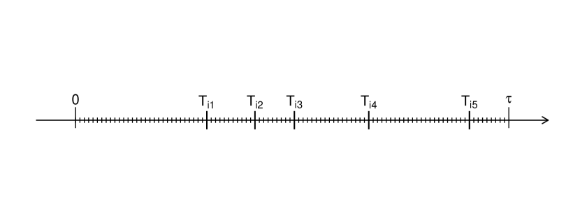
In the present work we consider a continuous-time model, utilizing a counting process framework (Andersen et al., 1993) where intensity processes define the rate of a finite number of continuous monitoring times for each subject conditional on their observed history, see Figure 1. Our approach is closely related to the work of Lok (2008) and of Røysland (2011, 2012), who propose continuous-time versions of structural nested models and marginal structural models (Robins, 1989b, a, 1992, 1998, 2000b, 2000a; Robins et al., 2000, 2008), respectively, using counting processes and martingale theory. Our parameter $\Psi(P_{0})$ is defined via the g-computation formula (Robins, 1986) in terms of interventions on the product integral representing the data-generating distribution.

To estimate $\Psi(P_{0})$, we proceed on the basis of the targeted minimum loss-based estimation (TMLE) framework (van der Laan and Rubin, 2006; van der Laan and Rose, 2011, 2018). TMLE is a general methodology for constructing regular and asymptotically linear substitution estimators for smooth low-dimensional parameters in infinite-dimensional models, combining flexible ensemble learning and semiparametric efficiency theory in a two-step procedure. The earliest of the TMLE developments for estimation of effects of time-varying treatments in longitudinal data structures (LTMLE) involve full likelihood estimation and targeting (van der Laan, 2010a, b; Stitelman et al., 2012) whereas the later (van der Laan and Gruber, 2012; Petersen et al., 2014) are based on the techniques of sequential regression originating from Bang and Robins (2005). All these methods rely on a discrete time-scale.

To construct our continuous-time TMLE algorithm we derive an expression for the efficient influence curve. The efficient influence curve is the canonical gradient of the functional $\Psi$ and is a central component in the construction of locally efficient estimators of a target parameter in general (Bickel et al., 1993). Semiparametric efficiency theory yields that, given a statistical model and a target parameter, a regular and asymptotically linear estimator is efficient if and only if its influence curve is equal to the efficient influence curve. Our estimation procedure is based on a representation of the target parameter in terms of intensities and conditional expectations for which we need initial estimators and a targeting updating algorithm. We propose such a targeting algorithm based on separate targeting steps for the intensities and for the conditional expectations that are iterated until convergence. The resulting estimator solves the efficient influence curve equation.

Our TMLE relies on initial estimators for the intensities and the conditional expectations that constitute our nuisance parameters. The TMLE framework allows us to take advantage of flexible and data-adaptive nuisance parameter estimation through super learning (van der Laan et al., 2007). A super learner is based on a library of candidate estimators for each nuisance parameter, and uses cross-validation to select the best combination of estimators. The general oracle inequality for cross-validation shows that the super learner performs asymptotically as well as the best combination of estimators in the library (van der Laan and Dudoit, 2003; van der Vaart et al., 2006). In particular, we discuss the highly adaptive lasso (HAL) (van der Laan, 2017) for all likelihood components. If this HAL estimator is included in the library of the super learner used for initial estimation, we can show that our TMLE estimator is asymptotically linear and efficient under minimal conditions on the model $\mathcal{M}$.

Refer to caption
Figure 1: Observations measured on a continuous scale, with five random time-points $T_{i1},\ldots,T_{i5}$ between time 00 and time $\tau$, referred to as monitoring times, where actual changes for the given subject $i$ are measured.

Our methods extend the existing longitudinal TMLE (LTMLE) to the continuous-time case. While the theory and asymptotic performance of LTMLE remain valid on any arbitrarily fine time-scale as long as it is discrete, we note the following. Sequential regression based LTMLE works by iterating through a sequence of regressions across all time-points and has been a popular choice over the full likelihood-based LTMLE that requires modeling of densities of potentially high-dimensional covariates. Our framework provides a unified methodology that covers both the continuous and the discrete-time case, where intensities of monitoring times are modeled separately and the regression approach can be used to deal with high-dimensional covariates. The substantial difference between LTMLE and our continuous-time TMLE lies in the limitation of LTMLE that one needs sufficiently many events at each time-point to fit the regressions. In contrast, our method can be applied when there are monitoring times with few events, or just one event.

1.1 Motivating applications

The methods developed here are applicable to a large variety of problems in pharmacoepidemiology. In this field of research, hazard ratios are often used as measures of the association of time-dependent exposure with time-to-event outcomes (see, e.g., Andersen et al., 2013; Karim et al., 2016; Kessing et al., 2019). However, the interpretation of hazard ratios as the measure of causal treatment effects is hampered for many reasons (Hernán, 2010; Martinussen et al., 2018). Furthermore, the time-dependent Cox model cannot be used in the presence of time-dependent confounding (Robins, 1986). In many applications, it is thus of great interest to formulate and estimate statistical parameters under hypothetical treatment interventions that have a causal interpretation under the right assumptions.

Specifically, it may be of interest to assess the effect of a (dynamic) drug treatment regime on the $\tau$-year risk of death. As an example, let $N^{a}(t)$ denote the process counting visits to a medical doctor who can prescribe the drug. Let the process $A(t)$ be information on the type and dose level of the drug prescribed at patient-specific times $T_{1}^{a}<T_{2}^{a}<\ldots<T^{a}_{N^{a}({\tau})}$ during the study period $[0,\tau]$. Further, let $N^{\ell}(t)$ denote the process counting doctor visits where health information $L(t)$ is collected. At visit $T^{a}_{k}$, the doctor considers the baseline characteristics $L_{0}$ of the patient, the treatment so far $\{(N^{a}(t),A(t)):t\in[0,T^{a}_{k-1}]\}$, and evaluates changes of covariates $\{(N^{\ell}(t),L(t)):t\in[0,T^{a}_{k})\}$ to decide to continue or to change the treatment. We are interested in the result of a hypothetical experiment that we would have liked to have conducted but did not. In our example, the causal effect resulting from such a hypothetical experiment could be the difference of the $\tau$-year risk of death under different (dynamic) treatment regimes.

A treatment regime is any a priori defined rule which can be applied at doctor visits during the study period to decide if the treatment should be changed or continued. For example, the intervention could state that the patient stays on an initially randomized drug throughout the entire study period. A dynamic treatment regime is an example of an adaptive intervention which allows the decision to depend on the current history of the patient. The rule could be that whenever the measurement of a blood marker value exceeds a certain threshold the dose level of the drug should be adapted. By comparison of the effects of different regimes we may further learn optimal strategies for treatment interventions based on patients’ medical past. In this article, we focus on interventions of the treatment process keeping the doctor visits where they naturally occur.

The data analysis is complicated by the fact that the observed data are subject to time-dependent confounding: At any point in time, doctors and patients make treatment decisions for reasons depending on treatment and covariate history. Furthermore, past treatment may further influence future values of covariates, such as biomarkers and diagnoses, and future treatment decisions. Additionally, a proportion of subjects in the population may be lost to follow-up (censored) which can likewise depend on prior treatment decisions and covariate values. Our estimation framework allows us to control for the history of all observed time-varying covariates and treatment choices that we believe could be predictive of both treatment decisions and censoring, and of the risk of death. Importantly, in the case where neither the treatment decision nor the censoring mechanism depend on any unrecorded health information, i.e., the observed history at any point in time is sufficient to predict the next treatment decision and the censoring at that time, the no unmeasured confounding assumption holds, and the estimated effects of hypothetical interventions based on the observed data can be interpreted causally.

1.2 Organization of article

The article is organized as follows. We first define the statistical estimation problem. Section 2 introduces the continuous-time longitudinal setting and presents the model of a single subject along with the likelihood. In particular, Section 2.2 defines interventions on the likelihood, Section 2.4 defines the target parameter, and Section 2.5 provides the efficient influence function for the estimation problem. In Section 2.4.1, we briefly review the assumptions under which the target parameter identifies the causal effect of interest. Section 3 presents a representation of the target parameter in terms of intensities and conditional expectations for which we need to construct an estimation procedure. Section 4 states a general theorem for asymptotically efficient substitution estimation. Section 5 introduces targeted minimum loss-based estimation (TMLE) for the considered estimation problem. Section 6 describes initial estimation of the likelihood components needed for the targeting updating steps and for estimation of the target parameter that fulfills the criteria of the efficiency theorem. Section 7 presents a particular TMLE algorithm for estimation of the target parameter in the continuous-time setting that involves separate targeting for conditional expectations and intensities, pooled over time. Section 8 reviews inference for the TMLE estimator. Section 9 presents the results of a simulation study as a demonstration of the methods and a proof-of-concept. Section 10 closes with a discussion.

2 Formulation of the statistical estimation problem

We start out defining the data structure, the statistical estimation problem and the target parameter. An overview of our notation can be found in Appendix C.1.

2.1 Notation and setup

We represent the subject-specific information in terms of a counting process model (Andersen et al., 1993). Suppose $n\in\mathbb{N}$ subjects of a population are followed in a bounded interval of time $[0,\tau]$. Let $(N^{a},N^{\ell},N^{c},N^{d})$ be a multivariate counting process generating random times at which treatment, covariates, censoring status and survival status may change. At jump times of $N^{a}$ we observe changes in a treatment regime $A(t)$ taking values in finite set $\mathcal{A}$ and at jump times of $N^{\ell}$ we observe changes of a covariate vector $L(t)$ with values in a compact subset of $\mathbb{R}^{d}$. The processes $N^{c}$ and $N^{d}$ generate changes in censoring status and death status, respectively. Furthermore, $L_{0}$ denotes a vector of baseline covariates measured at time 00, and $Y$ a real valued outcome variable measured at time $\tau$. We assume that there are no events at time zero, and that realizations of all processes are càdlàg functions on $[0,\tau]$. Let $(\mathcal{F}_{t})_{t\geq 0}$ denote the filtration generated by the history of the observed processes up to time $t$. Specifically, we have $\mathcal{F}_{0}=\sigma(L_{0})$.

Let $T_{1}^{a}<T_{2}^{a}<\ldots<T^{a}_{N^{a}({\tau})}$ and $T_{1}^{\ell}<T_{2}^{\ell}<\ldots<T^{\ell}_{N^{\ell}({\tau})}$ be the random times at which the treatment regime $A$ and the covariate process $L$ may change, and let $T^{c}$ and $T^{d}$ be the right-censoring time and the survival time, respectively. By definition, $N^{a}(t)$ and $N^{\ell}(t)$ are the subject-specific counts of treatment and covariate monitoring times in $[0,t]$. The actual end of follow-up for a subject is $\min(T^{c},T^{d},\tau)$ and the total number of unique event times before time $t$ is,

$$K(t)=\#\big{\{}\{T_{1}^{a},\ldots,T^{a}_{N^{a}(t)}\}\cup\{T_{1}^{\ell},\ldots,T^{\ell}_{N^{\ell}(t)}\}\cup\{T^{c},T^{d}\}\big{\}}.$$ (1)

For each subject, the number of change points of the multivariate counting process on $[0,\tau]$, $K=K({\tau})$, is finite.

For $x=a,\ell,d,c$, we denote by $\Lambda_{0}^{x}$ the cumulative intensity that characterizes the compensator of $N^{x}$. We further denote by $M^{x}=N^{x}-\Lambda_{0}^{x}$ the corresponding martingale. Heuristically, we have that

$\displaystyle P(N^{x}(dt)=1\,|\,\mathcal{F}_{t-})=\mathbb{E}[N^{x}(dt)\,|\,\mathcal{F}_{t-}]=d\Lambda_{0}^{x}(t\,|\,\mathcal{F}_{t-}),$

where the increment $N^{x}(dt)$ is non-zero and equal to 1 if and only if there is a jump of $N^{x}$ in the infinitesimal interval $[t,t+dt)$ (Andersen et al., 1993; Gill, 1994).

We assume that the processes $A$ and $L$ only change at monitoring times. The distribution of the treatment $A(t)$ at any time $t$ where $N^{a}(t)$ jumps is denoted $\pi_{0,t}(a\,|\,\mathcal{F}_{t-})=P(A(t)=a\,|\,\mathcal{F}_{t-})$, $a\in\mathcal{A}$, and the distribution of covariates $L(t)$ at any time $t$ where $N^{\ell}(t)$ jumps is characterized by a conditional density $\mu_{0,t}(\ell\,|\,\mathcal{F}_{t-})$ with respect to a dominating measure $\nu_{L}$. We assume that $A(t)=A(t-)$ and $L(t)=L(t-)$ otherwise. Lastly, the probability distribution of baseline covariates $L_{0}$ is characterized by the conditional density $\mu_{0,L_{0}}$ with respect to a dominating measure $\nu_{L_{0}}$.

2.1.1 Observations

For subject $i$, with $i=1,\dots,n$ independent subjects, let $\{T_{i,k}\}_{k=1}^{K_{i}(t)}$ denote the ordered set of unique event times up to time $t$. The observed data for subject $i$ in a bounded interval $[0,t]$, $t\leq\tau$, is given by:

$\displaystyle\bar{O}_{i}(t)=\big{\{}\big{(}L_{0,i},s,N_{i}^{a}(s),A_{i}(s),N_{i}^{\ell}(s),L_{i}(s),N_{i}^{d}(s),N_{i}^{c}(s)\big{)}\,:\,s\in\{T_{i,k}\}_{k=1}^{K_{i}(t)}\big{\}}.$ (2)

We also use the shorthand notation $O_{i}=\bar{O}_{i}(\tau)$ and denote by $\mathcal{O}$ the space where $O_{i}$ takes its values. Let $\mathbb{P}_{n}$ denote the empirical distribution of the data $\{O_{i}\}_{i=1}^{n}$. For a dataset with $n$ observations, we use,

$\displaystyle\qquad 0={t}_{0}<{t}_{1}<\cdots<{t}_{{K}_{n}},$ (3)

with ${K}_{n}=\sum_{i=1}^{n}K_{i}$, to denote the ordered sequence of unique times of changes $\cup_{i=1}^{n}\cup_{k=1}^{K_{i}}\{T_{i,k}\}$.

The distribution $P_{0}$ of the observed data $O$ factorizes according to the time-ordering, going from one infinitesimal time interval to the next with $d\Lambda_{0}^{x}(t\,|\,\mathcal{F}_{t-})$ representing the conditional probability of an event of $N^{x}$ in $[t,t+dt)$, for $x=a,\ell,d,c$ (Andersen et al., 1993, Section II.7). Accordingly, we express the likelihood as

$\displaystyle\begin{split}dP_{0}(O)=\qquad\qquad\qquad\qquad\qquad\qquad\qquad\qquad\qquad\qquad\qquad\qquad\qquad\qquad\qquad\\ \mu_{0,L_{0}}(L_{0})\Prodi_{t\in(0,\tau]}\big{(}d\Lambda_{0}^{\ell}(t\,|\,\mathcal{F}_{t-})\,\mu_{0,t}(L(t)\,|\,\mathcal{F}_{t-})\big{)}^{N^{\ell}(dt)}\big{(}1-d\Lambda_{0}^{\ell}(t\,|\,\mathcal{F}_{t-})\big{)}^{1-N^{\ell}(dt)}\\ \Prodi_{t\in(0,\tau]}\big{(}d\Lambda_{0}^{a}(t\,|\,\mathcal{F}_{t-})\,\pi_{0,t}(A(t)\,|\,\mathcal{F}_{t-})\big{)}^{N^{a}(dt)}\big{(}1-d\Lambda_{0}^{a}(t\,|\,\mathcal{F}_{t-})\big{)}^{1-N^{a}(dt)}\\ \Prodi_{t\in(0,\tau]}\big{(}d\Lambda_{0}^{c}(t\,|\,\mathcal{F}_{t-})\big{)}^{N^{c}(dt)}\big{(}1-d\Lambda_{0}^{c}(t\,|\,\mathcal{F}_{t-})\big{)}^{1-N^{c}(dt)}\\ \Prodi_{t\in(0,\tau]}\big{(}d\Lambda_{0}^{d}(t\,|\,\mathcal{F}_{t-})\big{)}^{N^{d}(dt)}\big{(}1-d\Lambda_{0}^{d}(t\,|\,\mathcal{F}_{t-})\big{)}^{1-N^{d}(dt)},\end{split}$ (4)

with $\prodi$ denoting the product integral (Gill and Johansen, 1990; Andersen et al., 1993, Section II.6). A particularly nice aspect of the product-integral representation is that it gives a unified presentation for the discrete and the continuous time case.

2.2 Interventions

We are interested in estimating the effect of dynamic treatment regimes (Robins, 2002; Murphy et al., 2001; Hernán et al., 2006; van der Laan and Petersen, 2007) corresponding to hypothetical experiments, under hypothetical interventions, where data had been generated differently. An intervention defines a rule specifying treatment at each intervention time point given the data so far. In our setting, we allow the number and schedule of the intervention time-points to be subject-specific and to occur in continuous time. We thus distinguish between interventions that control the treatment decision mechanism, but not the conditional distribution governing the schedule of the intervention time points, and interventions that control the distribution of treatment decisions as well as the distribution of the intervention times. In our motivating pharmacoepidemiological applications from Section 1.1, an intervention only on the treatment decision mechanism could for example specify a treatment regime where a particular drug treatment should be continued or discontinued, while the frequency of doctor visits are kept as they would naturally occur for the subjects of the population had they followed that treatment regime. In addition to the treatment regimes of interest, interventions always control the censoring mechanism, such that, in the hypothetical experiment, all subjects are followed for the entire study period $[0,\tau]$.

The observed data are generated by the distribution $P_{0}$ which factorizes as displayed in (4). We define interventions directly on $P_{0}$, by replacing a subset of its components by an intervention-specific choice. To formulate this, we decompose the observed data distribution $P_{0}$ into two parts which we refer to as the interventional part ($G_{0}$) and the non-interventional part ($Q_{0}$), respectively. We parametrize $P_{0}$ accordingly,

$\displaystyle d{P}_{0}=d{P_{Q_{0},G_{0}}}=\Prodi_{t\in[0,\tau]}dQ_{0,t}\,dG_{0,t},$

with $dG_{0,t}(o)$ and $dQ_{0,t}(o)$ denoting the conditional measures, given the observed history, corresponding to the interventional part and the non-interventional part at time $t$, respectively. We use $g_{0,t}$ to denote the density of $G_{0,t}$ and likewise $q_{0,t}$ to denote the density of $Q_{0,t}$, both with respect to appropriate dominating measures.

Now, an intervention involves replacing $G_{0}$ by some $G^{*}$ encoding how treatment and censoring is generated conditional on the available history in the hypothetical experiment. In its generality, this is what is referred to as a randomized plan in Gill and Robins (2001, Sections 6 and 7), or a stochastic intervention (Robins et al., 2004; Dawid and Didelez, 2010), but it includes static and dynamic interventions (Hernán et al., 2006; Chakraborty and Moodie, 2013) plans as special cases as we explain below. Which components we include in $G_{0}$, and thus intervene upon, depends on what kinds of effects we are interested in and thus what scientific question we wish to address. Consider the following options.

Definition 1 (Interventions on treatment assigned).

An intervention on treatment assigned involves replacing $\pi_{0,t}$ by some choice $\pi_{t}^{*}$. Thus, the interventional part includes the treatment and the censoring mechanism:

$\displaystyle\begin{split}dG_{0,t}(O)=\big{(}\pi_{0,t}(A(t)\,|\,\mathcal{F}_{t-})\big{)}^{N^{a}(dt)}\big{(}d\Lambda_{0}^{c}(t\,|\,\mathcal{F}_{t-})\big{)}^{N^{c}(dt)}\\ \big{(}1-d\Lambda_{0}^{c}(t\,|\,\mathcal{F}_{t-})\big{)}^{1-N^{c}(dt)}.\end{split}$ (5)

The intervention prevents censoring and specifies the treatment regime $\pi_{t}^{*}$, such that

$$dG_{t}^{*}(O)=\big{(}1-N^{c}(t))\,\pi_{t}^{*}(A(t)\,|\,\mathcal{F}_{t-}).$$

The distribution of the intervention times is not intervened upon, i.e., $\Lambda_{0}^{a}$ is included in the non-interventional part.

When the interventional treatment distributions are degenerated and, for example, set to a single value $a^{*}\in\mathcal{A}$ throughout the entire study period,

$\displaystyle\pi_{t}^{*}(A(t)\,|\,\mathcal{F}_{t-})=\mathbb{1}\{A(t)=a^{*}\}.$ (6)

We refer to $\pi_{t}^{*}$ as a static intervention since it deterministically sets $A(t)=a^{*}$ (at treatment monitoring times). A dynamic intervention, on the other hand, defines $\pi^{*}_{t}$ that assigns $A(t)$ deterministically dependent on the subject’s observed past.

Definition 2 (Intervention on treatment and schedule).

The interventional part includes the treatment, the schedule of intervention times, and the censoring mechanism:

$\displaystyle\begin{split}dG_{0,t}(O)=\big{(}d\Lambda_{0}^{a}(t\,|\,\mathcal{F}_{t-})\,\pi_{0,t}(A(t)\,|\,\mathcal{F}_{t-})\big{)}^{N^{a}(dt)}\big{(}1-d\Lambda_{0}^{a}(t\,|\,\mathcal{F}_{t-})\big{)}^{1-N^{a}(dt)}\\ \big{(}d\Lambda_{0}^{c}(t\,|\,\mathcal{F}_{t-})\big{)}^{N^{c}(dt)}\big{(}1-d\Lambda_{0}^{c}(t\,|\,\mathcal{F}_{t-})\big{)}^{1-N^{c}(dt)}.\end{split}$

The intervention prevents censoring and specifies a treatment regime by $\pi_{t}^{*}$ and $\Lambda^{a,*}$, such that,

$\displaystyle dG^{*}_{t}(O)=\big{(}d\Lambda^{a,*}(t\,|\,\mathcal{F}_{t-})\,\pi^{*}_{t}(A(t)\,|\,\mathcal{F}_{t-})\big{)}^{N^{a}(dt)}\big{(}1-d\Lambda^{a,*}(t\,|\,\mathcal{F}_{t-})\big{)}^{1-N^{a}(dt)}.$

An intervention on the schedule of treatment decisions involves replacing the intensity $\Lambda_{0}^{a}$ by some choice $\Lambda^{a,*}$. In the context of the applications described in Section 1.1, this could be to decrease or increase the frequency of doctor visits, for instance to ensure at least a monthly visit.

To focus our presentation, we continue with $dG_{0,t}$ as defined by (5) according to Definition 1, considering interventions only on the treatment decision $\pi_{t}$ and on the censoring mechanism $\Lambda^{c}$. Note that this defines the non-interventional part as

$\displaystyle dQ_{0,t}(O)$ $\displaystyle=\big{(}d\Lambda_{0}^{a}(t\,|\,\mathcal{F}_{t-})\big{)}^{N^{a}(dt)}\big{(}1-d\Lambda_{0}^{a}(t\,|\,\mathcal{F}_{t-})\big{)}^{1-N^{a}(dt)}$
$\displaystyle\qquad\big{(}d\Lambda_{0}^{\ell}(t\,|\,\mathcal{F}_{t-})\,\mu_{0,t}(L(t)\,|\,\mathcal{F}_{t-})\big{)}^{N^{\ell}(dt)}\big{(}1-d\Lambda_{0}^{\ell}(t\,|\,\mathcal{F}_{t-})\big{)}^{1-N^{\ell}(dt)}$
$\displaystyle\qquad\big{(}d\Lambda_{0}^{d}(t\,|\,\mathcal{F}_{t-})\big{)}^{N^{d}(dt)}\big{(}1-d\Lambda_{0}^{d}(t\,|\,\mathcal{F}_{t-})\big{)}^{1-N^{d}(dt)},$

for $t>0$.

2.3 Statistical model

Let $\mathcal{Q}$ denote the parameter set for the non-interventional part $Q=(\mu_{t},{\Lambda}^{a}(t),$ $\Lambda^{\ell}(t),\Lambda^{d}(t))_{t\in[0,\tau]}$ and $\mathcal{G}$ the parameter set for the interventional part $G=(\pi_{t},{\Lambda}^{c}(t))_{t\in[0,\tau]}$. We consider a statistical model $\mathcal{M}$ as follows:

$\displaystyle\mathcal{M}=\bigg{\{}P\,:\,dP=dP_{Q,G}=\Prodi_{t\in[0,\tau]}dQ_{t}dG_{t},\,\,G\in\mathcal{G},\,Q\in\mathcal{Q}\bigg{\}}.$ (7)

In Section 6 we summarize results that require $Q,G$ to be contained in the set of càdlàg functions, i.e., functions that are right-continuous with left-hand limits, with bounded sectional variation norm. For now we leave $\mathcal{Q},\mathcal{G}$ unspecified.

2.4 Target parameter

Suppose an intervention $G^{*}$ is given. We define the post-interventional distribution for any $P\in\mathcal{M}$ by replacing $G$ by $G^{*}$ in $P_{Q,G}$. The resulting $P_{Q,G^{*}}$ is commonly referred to as the g-computation formula (Robins, 1986; Gill and Robins, 2001). We will also denote this by $P^{G^{*}}$. Based on the data $O=\bar{O}(\tau)$, our overall aim is to estimate the expectation of the outcome of interest $Y$ under the g-computation formula. That is, we are interested in the parameter $\Psi^{G^{*}}\,:\,\mathcal{M}\rightarrow\mathbb{R}$ given by

$\displaystyle\Psi^{G^{*}}(P)=\mathbb{E}_{P^{G^{*}}}\big{[}Y\big{]}=\int_{{\mathcal{O}}}y\,\Prodi_{t\in[0,\tau]}dQ_{t}(o)\,dG_{t}^{*}(o),$ (8)

where the notation $\mathbb{E}_{P^{G^{*}}}$ refers to the expectation operator with respect to the post-interventional measure $P^{G^{*}}=P_{Q,G^{*}}$.

In this paper we focus on an all-cause mortality outcome, $Y={N}^{d}(\tau)$, so that (8) is the expected risk of dying by time $\tau$ under the distribution defined by the g-computation formula. We emphasize, however, that in principle $Y$ can be defined as any mapping of the observed past $\mathcal{F}_{\tau}$ as long as $Y$ takes value in a compact set. We denote by $\psi_{0}:=\Psi^{G^{*}}(P_{0})$, the true value of the target parameter. The target parameter is identifiable from the observed data under the following positivity assumption.

Assumption 1 (Positivity).

We assume absolute continuity of $P_{Q,{G}^{*}}$ with respect to $P_{Q,{G}}$, i.e., $P_{Q,{G}^{*}}\ll P_{Q,{G}}$. This implies existence of the Radon-Nikodym derivative $dP_{Q,{G}^{*}}/dP_{Q,{G}}=\prodi_{s<\tau}dG^{*}_{s}/dG_{s}$.

The g-computation formula arising from replacing the observed $G_{0}$ by $G^{*}$ and the resulting target parameter in (8) are well-defined statistical quantities by Assumption 1.

2.4.1 Causal parameter and causal interpretability

Causal interpretability of the g-computation formula in the setting of discrete data is provided by Robins’ work (Robins, 1986, 1987, 1989b) under the assumptions of no unmeasured confounding and positivity (for a nice review, see, Hernan and Robins, 2020, Part III). This work is further generalized by Gill and Robins (2001) to continuously varying covariates and treatments. Our setting differs from theirs in that subjects are measured at random times on a continuous scale: Our g-computation formula is represented as a product integral over times where something actually happens, whereas the g-computation formula of Gill and Robins (2001) consists of a finite product over times of a discrete grid. Nevertheless, note that the counting processes only have finitely many changes in the compact time interval $[0,\tau]$, and that interventions on the treatment decision are in fact only applied at a finite number of (random) times. Thus, the ‘traditional’ causal assumptions as stated by Gill and Robins (2001) can be applied at the random times to ensure the causal interpretation of the g-computation formula (Gill and Robins, 2001, Theorem 2).

Particularly, consider $G^{*}$ that defines an intervention on the treatment assigned according to a distribution $\pi^{*}_{t}$. Let $O^{G^{*}}$ be the counterfactual random variable representing the data that would have been observed, had $G^{*}$ been adhered to rather than the factual $G$ throughout the follow-up period. The causal parameter of interest is $\mathbb{E}[Y^{G^{*}}]$, the expected value of $Y$ when imposing the intervention $G^{*}$. For our setting with random treatment monitoring times, $T_{1}^{a}<T_{2}^{a}<\ldots<T^{a}_{N^{a}({\tau})}$, we formulate the no unmeasured confounding assumption for the treatment decision as follows:

Assumption 2 (No unmeasured confounding).

$Y^{G^{*}}\!\mathchoice{\mathrel{\hbox to0.0pt{$\displaystyle\perp$\hss}\mkern 2.0mu{\displaystyle\perp}}}{\mathrel{\hbox to0.0pt{$\textstyle\perp$\hss}\mkern 2.0mu{\textstyle\perp}}}{\mathrel{\hbox to0.0pt{$\scriptstyle\perp$\hss}\mkern 2.0mu{\scriptstyle\perp}}}{\mathrel{\hbox to0.0pt{$\scriptscriptstyle\perp$\hss}\mkern 2.0mu{\scriptscriptstyle\perp}}}A(T^{a}_{k})\,|\,\bar{O}(T^{a}_{k}-)$, for all $k=1,\ldots,N^{a}({\tau})$.

Assumption 1 and Assumption 2 together yield that our target parameter identifies the expected value of the counterfactual outcome, i.e., $\Psi^{G^{*}}(P)=\mathbb{E}[Y^{G^{*}}]$, had the treatment decisions been governed by $\pi^{*}_{t}$.

In settings where one intervenes not only on the treatment decisions but also on the mechanism of the timing of treatment monitoring, an additional assumption equivalent to Assumption 2 is needed. Specifically, causal interpretability of $\Psi^{G^{*}}(P)$ is in that case achieved if the counterfactual outcome $Y^{G^{*}}$ is independent of the time to the next treatment monitoring event conditional on the observed history up to any event time $T_{k}$.

2.5 Canonical gradient

The canonical gradient of the pathwise derivative of the target parameter characterizes the information bound of the estimation problem relative to the statistical model $\mathcal{M}$ (Bickel et al., 1993). The canonical gradient is also known as the efficient influence curve. The following theorem provides a representation of the canonical gradient for our statistical model $\mathcal{M}$ and target parameter $\Psi^{G^{*}}\,:\,\mathcal{M}\rightarrow\mathbb{R}$. We will use this representation to construct an asymptotically efficient estimator.

We follow a general recipe to derive our expression for the canonical gradient. For this, consider the submodel $\mathcal{M}_{G}\subset\mathcal{M}$ that assumes $G$ to be known and let $\mathscr{T}_{G}(P)$ denote the tangent space at $P$ in the submodel $\mathcal{M}_{G}$. The canonical gradient can be found as the projection of any other gradient of the pathwise derivative of $\Psi\,:\,\mathcal{M}_{G}\rightarrow\mathbb{R}$ at $P$ onto the tangent space $\mathscr{T}_{G}(P)$ (van der Laan and Robins, 2003). Thus, we need to characterize the tangent space $\mathscr{T}_{G}(P)$ and construct an initial gradient to project onto $\mathscr{T}_{G}(P)$. Note that the tangent space $\mathscr{T}_{G}(P)$ is generated by fluctuations only of the conditional distributions of $Q$ since $G$ is known. To construct an initial gradient, we can use the influence curve of an inverse probability weighted estimator of $\psi_{0}$ in $\mathcal{M}_{G}$. The detailed derivations can be found in Appendix A.

Theorem 1 (Canonical gradient).

The canonical gradient $D^{*}(P)$ at $P$ in $\mathcal{M}$ can be represented as follows:

$\displaystyle D^{*}(P)=\mathbb{E}_{P^{G^{*}}}[Y\,|\,\mathcal{F}_{0}]-\Psi^{G^{*}}(P)$
$\displaystyle\,\,\,+\,\int_{0}^{\tau}\Prodi_{s<t}\frac{dG^{*}_{s}}{dG_{s}}\Big{(}\mathbb{E}_{P^{G^{*}}}[Y\,|\,L(t),N^{\ell}(t),\mathcal{F}_{t-}]-\mathbb{E}_{P^{G^{*}}}[Y\,|\,N^{\ell}(t),\mathcal{F}_{t-}]\Big{)}N^{\ell}(dt)$
$\displaystyle\,+\,\int_{0}^{\tau}\Prodi_{s<t}\frac{dG^{*}_{s}}{dG_{s}}\Big{(}\mathbb{E}_{P^{G^{*}}}[Y\,|\,\Delta N^{\ell}(t)=1,\mathcal{F}_{t-}]-\mathbb{E}_{P^{G^{*}}}[Y\,|\,\Delta N^{\ell}(t)=0,\mathcal{F}_{t-}]\Big{)}M^{\ell}(dt)$
$\displaystyle\,+\,\int_{0}^{\tau}\Prodi_{s<t}\frac{dG^{*}_{s}}{dG_{s}}\Big{(}\mathbb{E}_{P^{G^{*}}}[Y\,|\,\Delta N^{a}(t)=1,\mathcal{F}_{t-}]-\mathbb{E}_{P^{G^{*}}}[Y\,|\,\Delta N^{a}(t)=0,\mathcal{F}_{t-}]\Big{)}M^{a}(dt)$
$\displaystyle\,+\,\int_{0}^{\tau}\Prodi_{s<t}\frac{dG^{*}_{s}}{dG_{s}}\Big{(}1-\mathbb{E}_{P^{G^{*}}}[Y\,|\,N^{d}(t)=0,\mathcal{F}_{t-}]\Big{)}M^{d}(dt).$

We here follow notation of Andersen et al. (1993) and use $\Delta$ to denote the difference operator defined by $\Delta X=X-X_{-}$ for a càdlàg process $X$.

3 Representation of the target parameter by iterated expectations

Estimation of the target parameter requires evaluation of a large integral. We here present a parametrization of the target parameter in terms of a nested sequence of conditional expectations which is central for our estimation procedure. As for the discrete-time analogue (Bang and Robins, 2005; Robins, 2000b), the parametrization is defined backwards through time, starting at the end of the study period $\tau$. The main difference to the discrete-time representation is that the time-points where events happen are random.

The notation that we present in this section will be used throughout the remainder of the paper. For $P\in\mathcal{M}$ and a fixed regime $G^{*}$ according to Definition 1, we define for $t\in[0,\tau]$:

$\displaystyle Z_{t}^{G^{*}}$ $\displaystyle:=\mathbb{E}_{P^{G^{*}}}\big{[}Y\,\big{|}\,L(t),N^{\ell}(t),N^{a}(t),N^{d}(t),\mathcal{F}_{t-}\big{]}=\int Y\,\Prodi_{s\geq t}dG^{*}_{s}\,\Prodi_{s>t}dQ_{s}.$ (9)

Note that the conditioning set of $Z_{t}^{G^{*}}$ excludes the interventional part at time $t$. We further denote the conditional expectation where $L(t)$ has been integrated out by:

$\displaystyle\begin{split}Z_{t,L(t)}^{G^{*}}:=&\,\mathbb{E}_{P^{G^{*}}}\big{[}Y\,\big{|}\,N^{\ell}(t),N^{a}(t),N^{d}(t),\mathcal{F}_{t-}\big{]}\\[3.00003pt] =&\,\mathbb{E}_{P^{G^{*}}}\big{[}Z_{t}^{G^{*}}\,\big{|}\,N^{\ell}(t),N^{a}(t),N^{d}(t),\mathcal{F}_{t-}\big{]}\\ =&\,\int\bigg{(}\int Y\,\Prodi_{s\geq t}dG^{*}_{s}\,\Prodi_{s>t}dQ_{s}\bigg{)}d\mu_{0,t}(L(t)\,|\,\mathcal{F}_{t-}).\end{split}$ (10)

The notation using the subscript ‘$L(t)$’ in $Z_{t,L(t)}^{G^{*}}$ to refer to $L(t)$ being integrated out follows the notation of van der Laan and Gruber (2012).

Lemma 1.

Define, for any $P\in\mathcal{M}$:

$\displaystyle{\bm{Z}}={\bm{Z}}(P):=\big{(}{Z}^{G^{*}}_{t},{Z}^{G^{*}}_{t,L(t)},{\Lambda}^{\ell}(t),{\Lambda}^{a}(t),{\Lambda}^{d}(t)\big{)}_{t\in[0,\tau]}.$ (11)

Particularly, let $\bm{Z}_{0}={\bm{Z}}(P_{0})$. The target parameter $\Psi^{G^{*}}$ defined in (8) can be represented as a functional of $P$ only through $\bm{Z}$.

Proof.

See Appendix A.8. ∎

In line with the sequential regression representation of Bang and Robins (2005), we may thus utilize that $\bm{Z}$ rather than $P$ itself can be used to evaluate the target parameter. Our aim is to estimate $\bm{Z}$ in an optimal way. The canonical gradient presented in Theorem 1 can be represented as a functional of $\bm{Z}$ and $G$; this will guide the construction of estimators for $\bm{Z}$ as a result of our efficiency theorem in Section 4.

4 Efficiency theorem for substitution estimation

In the previous section we have demonstrated that the target parameter can be represented as a functional of $P\in\mathcal{M}$ through $\bm{Z}$. We define a substitution estimator of the target parameter $\psi_{0}=\Psi(P_{0})$ based on an estimator $\hat{\bm{Z}}_{n}$ for $\bm{Z}_{0}$. The following theorem states the general conditions for asymptotic efficiency of such substitution estimation of $\psi_{0}$. Particularly, efficient estimation requires estimation of the relevant parts of the data-generating distribution that enter the expression of the efficient influence curve. Thus, an efficient estimator $\hat{P}_{n}$ is characterized by both $\hat{\bm{Z}}_{n}$ and $\hat{G}_{n}$. The proof of the theorem follows proofs in similar work (see, e.g., van der Laan and Rubin, 2006; van der Laan, 2017; van der Laan and Rose, 2011, Theorem A.5), is short and relies on an analysis of the separate terms of a von Mises expansion of the target parameter. In Section 6 we summarize results on initial estimators that meet the regularity conditions under minimal smoothness conditions on $\mathcal{M}$. Throughout we use the notation $Pf=\int fdP$ and $\|f\|_{P}=\sqrt{Pf^{2}}$.

We show in Appendix A.7 that the difference $\Psi^{G^{*}}(P)-\Psi^{G^{*}}(P_{0})$ admits the following presentation:

$\displaystyle\Psi^{G^{*}}(P)-\Psi^{G^{*}}(P_{0})=-P_{0}D^{*}(P)+R_{2}(P,P_{0}),\qquad P\in\mathcal{M},$ (12)

where $D^{*}(P)$ is the canonical gradient and the second-order remainder $R_{2}(P,P_{0})$ is given by:

$\displaystyle\begin{split}&R_{2}(P,P_{0})=\Psi^{G^{*}}(P)-\Psi^{G^{*}}(P_{0})+P_{0}D^{*}(P)\\ &\,=\int_{0}^{\tau}\int_{\mathcal{O}}Y\,\frac{1}{{\bar{g}}_{t}}\big{(}\bar{g}_{0,t}-{\bar{g}}_{t}\big{)}\Prodi_{s\leq\tau}dG_{s}^{*}\Prodi_{s<t}dQ_{0,s}\,\big{(}dQ_{0,t}-d{Q}_{t}\big{)}\Prodi_{s>t}d{Q}_{s}.\end{split}$ (13)

Here we have used the notation:

$\displaystyle\bar{g}_{t}=\Prodi_{s<t}g_{s},\quad\text{and,}\quad\bar{g}_{0,t}=\Prodi_{s<t}g_{0,s},$

with ${g}_{t}$ being the density of the interventional part $dG_{t}$ as defined in Section 2.2.

Theorem 2.

Consider an estimator $\hat{P}_{n}$ for $P_{0}$, such that

$\displaystyle\mathbb{P}_{n}D^{*}(\hat{P}_{n})=o_{P}(n^{-1/2}).$ (14)

If the following conditions 1 and 2 hold true,

  1. Condition 1)

    $R_{2}(\hat{P}_{n},P_{0})=o_{P}(n^{-1/2})$,

  2. Condition 2)

    $D^{*}(\hat{P}_{n})$ belongs to a Donsker class, and $P_{0}\big{(}D^{*}(\hat{P}_{n})-D^{*}(P_{0})\big{)}^{2}$ converges to zero in probability,

then

$\displaystyle\Psi^{G^{*}}(\hat{P}_{n})-\Psi^{G^{*}}(P_{0})=\mathbb{P}_{n}D^{*}(P_{0})+o_{P}(n^{-1/2}),$

that is, $\Psi^{G^{*}}(\hat{P}_{n})$ is asymptotically linear at $P_{0}$ with influence curve $D^{*}(P_{0})$ and is thus asymptotically efficient among all locally regular estimators at $P_{0}$.

Proof.

The proof of the theorem relies on the expansion (12). Applying the representation at $\hat{P}_{n}^{*}$ and using Equation (14) from the theorem yields

$\displaystyle\Psi^{G*}(\hat{P}_{n})-\Psi^{G*}(P_{0})={(\mathbb{P}_{n}-P_{0})D^{*}(\hat{P}_{n})}+R_{2}(\hat{P}_{n},P_{0})+o_{P}(n^{-1/2}).$

It is now a result of empirical process theory (see, e.g., van der Vaart, 2000, Lemma 19.24) that condition 2 implies

$\displaystyle{(\mathbb{P}_{n}-P_{0})\big{(}D^{*}(\hat{P}_{n})-D^{*}({P}_{0})\big{)}}=o_{P}(n^{-1/2}),$

which finishes the proof. ∎

If we are able to construct estimators $\hat{P}_{n}$ that meet the conditions of Theorem 2 and solve Equation (14), the so-called efficient influence curve equation, then the resulting substitution estimator $\Psi^{G^{*}}(\hat{P}_{n})$ is asymptotically linear and efficient. In the following, we comment on conditions 1 and 2.

Remark 1 (Second-order remainder).

The second-order remainder expressed in (13) displays a double robustness structure (van der Laan and Robins, 2003) in the sense that,

$\displaystyle R_{2}(P,P_{0})=0\quad\text{if}\quad\bar{g}_{t}=\bar{g}_{0,t}\quad\text{or}\quad q_{t}=q_{0,t}.$

When ${\bar{G}}_{t}$ is bounded away from zero, the product structure of the remainder $R_{2}(P,P_{0})$ yields, by use of the Cauchy-Schwartz inequality, an upper bound in terms of the $L_{2}(P_{0})$-norm of $(\bar{g}_{0,t}-{\bar{g}}_{t})$ and the $L_{2}(P_{0})$-norm of $({q}_{0,t}-{{q}}_{t})$:

$\displaystyle\int_{0}^{\tau}\|\bar{g}_{0,t}-\bar{g}_{t}\|_{P_{0}}\,\|q_{0,t}-q_{t}\|_{P_{0}}\,dt.$

Here we have further used that $Y\in[0,1]$. The required convergence rate $R_{2}(\hat{P}_{n},P_{0})=o_{P}(n^{-1/2})$ will for example be achieved if we estimate both parts at a rate faster than $o_{P}(n^{-1/4})$. In Section 6 we apply recent results on highly adaptive lasso (HAL) estimation (van der Laan, 2017) to show that such estimators do exist.

Remark 2 (Donsker class conditions).

In Section B.1 we give conditions under which $D^{*}(\hat{P}_{n})\in\mathscr{F}$ where $\mathscr{F}=\{D^{*}(P)\,:\,P\}$ is a Donsker class. The key is that there is a finite number of monitoring times per subject, so that any subject contributes with finitely many terms to the likelihood. Then the canonical gradient can be written as a well-behaved mapping of the nuisance parameters such that Donsker properties of the nuisance parameters will translate into Donsker properties of the efficient influence curve. An important Donsker class is the class of càdlàg functions with finite variation.

Theorem 2 tells us what we need for efficient estimation of our target parameter. The next sections deal with construction of such an estimator.

5 Targeted minimum loss-based estimation (TMLE)

We present a TMLE procedure for construction of an estimator that will satisfy the conditions of Theorem 2. In summary, this consists of, first, constructing initial estimators for the components of $\bm{Z}$ and $G$, and, second, setting up an algorithm for performing an update of the collection of initial estimators that guarantees that it solves the efficient influence curve equation (14).

We also refer to the second step as the targeting step or the targeting algorithm. It involves for each component of $\bm{Z}$ a choice of a loss function and a corresponding path indexed by $\varepsilon\in\mathbb{R}$ through the initial estimator of that component such that the generated score at $\varepsilon=0$ gives a desired part of the canonical gradient. The general targeting algorithm involves iterative updating steps that are repeated until convergence, at which point the efficient influence curve equation (14) is solved.

A certain amount of extra notation is needed. For $t\in(0,\tau]$, we define the “clever weights” as the Radon-Nikodym derivative

$\displaystyle h^{G^{*}}_{t}$ $\displaystyle=\Prodi_{s<t}\frac{dG^{*}_{s}}{dG_{s}},$ (15)

that only depends on the $G$-part of the likelihood, and the “clever covariates”,

$\displaystyle h^{\ell}_{t}$ $\displaystyle=\mathbb{E}_{P^{G^{*}}}[Y\,|\,\Delta N^{\ell}(t)=1,\mathcal{F}_{t-}]-\mathbb{E}_{P^{G^{*}}}[Y\,|\,\Delta N^{\ell}(t)=0,\mathcal{F}_{t-}],$ (16)
$\displaystyle h^{a}_{t}$ $\displaystyle=\mathbb{E}_{P^{G^{*}}}[Y\,|\,\Delta N^{a}(t)=1,\mathcal{F}_{t-}]-\mathbb{E}_{P^{G^{*}}}[Y\,|\,\Delta N^{a}(t)=0,\mathcal{F}_{t-}],$ (17)
$\displaystyle h^{d}_{t}$ $\displaystyle=1-\mathbb{E}_{P^{G^{*}}}[Y\,|\,N^{d}(t)=0,\mathcal{F}_{t-}],$ (18)

that only depend on $\bm{Z}$. This now allows us to write the canonical gradient as,

$\displaystyle D^{*}(P)=Z^{G^{*}}_{t=0}-\Psi^{G^{*}}(P)$
$\displaystyle\qquad+\,\int_{0}^{\tau}h^{G^{*}}_{t}\big{(}Z_{t}^{G^{*}}-Z_{t,L(t)}^{G^{*}}\big{)}dN^{\ell}(t)+\sum_{x\in\{a,\ell,d\}}\int_{0}^{\tau}h^{G^{*}}_{t}\,h^{x}_{t}\,dM^{x}(t).$ (19)

In the following, we define loss functions and one-dimensional parametric submodels for each component of $\bm{Z}$ such that the scores are equal to the respective terms of (19). These will be used to construct our targeting algorithm in Section 7. We consider each term of (19) separately and define loss functions and submodels for $Z^{G^{*}}_{t,L(t)}$ (Section 5.1) and for each of the conditional intensities $\Lambda^{x}$, $x=a,\ell,d$ (Section 5.2).

Before we do so, we remark upon another particular approach taken in the discrete-time setting (van der Laan, 2010a; Stitelman et al., 2012) that could also be applied to our problem. Note that, in this paper, we focus on the parametrization of the target parameter $\Psi^{G^{*}}$ in terms of $\bm{Z}$ as presented in Section 3, but we could instead construct initial estimators for all likelihood components, i.e., all conditional densities and intensities, and construct a targeted updating step for each of these components as is done in the discrete-time case. Here we focus on $\bm{Z}$ rather than the full likelihood so that we can avoid targeting the conditional density of the potential high-dimensional $L(t)$. This will make the targeting step simpler and computationally more efficient.

5.1 Loss function and submodel for $Z^{G^{*}}_{t,L(t)}$

We need a loss function and a submodel for $Z^{G^{*}}_{t,L(t)}$ such that the score of the submodel equals the first term of (19). This term consists of an integral over a difference between $Z_{t}^{G^{*}}$ and $Z_{t,L(t)}^{G^{*}}$; thus, we will define our loss function and submodel for $Z^{G^{*}}_{t,L(t)}$ for a given $Z_{t}^{G^{*}}$. Particularly, we define the time-point specific logarithmic loss for ${Z}_{t,L(t)}^{G^{*}}$, indexed by ${Z}_{t}^{G^{*}}$:

$$\mathscr{L}_{t,{Z}_{t}^{G^{*}}}\big{(}{Z}_{t,L(t)}^{G^{*}}\big{)}={Z}^{G^{*}}_{t}\log{Z}^{G^{*}}_{t,L(t)}+\big{(}1-{Z}^{G^{*}}_{t}\big{)}\log\big{(}1-{Z}^{G^{*}}_{t,L(t)}\big{)}.$$

With this loss function, the parametric submodel

$$\text{logit}\,{Z}^{G^{*}}_{t,L(t)}(\varepsilon)=\text{logit}\,{Z}^{G^{*}}_{t,L(t)}+\varepsilon h_{t}^{G^{*}},$$

has the desired property that

$$\frac{d}{d\varepsilon}\,\mathscr{L}_{t,{Z}_{t}^{G^{*}}}\big{(}{Z}_{t,L(t)}^{G^{*}}(\varepsilon)\big{)}\,\Big{|}_{\varepsilon=0}={h}^{G^{*}}_{t}\,\big{(}{Z}^{G^{*}}_{t}-{Z}^{G^{*}}_{t,L(t)}\big{)}.$$

Correspondingly, we define the integrated loss for ${\bar{Z}}^{G^{*}}_{\tau,L(\tau)}=({Z}^{G^{*}}_{s,L(s)}\,:\,0\leq s\leq\tau)$, indexed by ${\bar{Z}}^{G^{*}}_{\tau}=({Z}^{G^{*}}_{s}\,:\,0\leq s\leq\tau)$,

$\displaystyle\bar{\mathscr{L}}_{{\bar{Z}}_{\tau}^{G^{*}}}\big{(}{\bar{Z}}_{\tau,L(\tau)}^{G^{*}}(\varepsilon)\big{)}=\int_{0}^{\tau}\mathscr{L}_{t,{Z}_{t}^{G^{*}}}\big{(}{Z}_{t,L(t)}^{G^{*}}(\varepsilon)\big{)}\,dN^{\ell}(t),$

for which we have that

$\displaystyle\frac{d}{d\varepsilon}\bar{\mathscr{L}}_{{\bar{Z}}_{\tau}^{G^{*}}}\big{(}{\bar{Z}}_{\tau,L(\tau)}^{G^{*}}(\varepsilon)\big{)}\,\Big{|}_{\varepsilon=0}$ $\displaystyle=\int_{0}^{\tau}\frac{d}{d\varepsilon}\,\mathscr{L}_{t,{Z}_{t}^{G^{*}}}\big{(}{Z}_{t,L(t)}^{G^{*}}(\varepsilon)\big{)}\,\Big{|}_{\varepsilon=0}\,dN^{\ell}(t)$
$\displaystyle=\int_{0}^{\tau}{h}^{G^{*}}_{t}\,\big{(}{Z}^{G^{*}}_{t}-{Z}^{G^{*}}_{t,L(t)}\big{)}\,dN^{\ell}(t),$

which, as we wanted, equals the first term of the part of the canonical gradient expressed in (19).

5.2 Loss function and submodel for the intensities ${\Lambda}^{x}(t)$

We consider the case that $\Lambda^{x}$ is absolutely continuous and denote by $\lambda^{x}$ the intensity rate such that $\Lambda^{x}(t\,|\,\mathcal{F}_{t-})$ $=\int_{0}^{t}\lambda^{x}(s\,|\,\mathcal{F}_{s-})ds$. For each $x=a,\ell,d$, we specify a proportional hazard type submodel for $\Lambda^{x}$ with time-dependent covariates as follows:

$\displaystyle\begin{split}d\Lambda^{x}(t;\varepsilon)&=d\Lambda^{x}(t)\exp(\varepsilon{h}^{G^{*}}_{t}{h}^{x}_{t}),\end{split}$ (20)

together with the partial log-likelihood loss function:

$\displaystyle\mathscr{L}_{x}({\Lambda}^{x})$ $\displaystyle=\log\bigg{(}\Prodi_{t\in[0,\tau]}\big{(}\lambda^{x}(t)\big{)}^{N^{x}(dt)}\big{(}1-d\Lambda^{x}(t)\big{)}^{1-N^{x}(dt)}\bigg{)}$
$\displaystyle=\int_{0}^{\tau}\log\lambda^{x}(t)\,dN^{x}(t)-\int_{0}^{\tau}d\Lambda^{x}(t).$

For this pair of submodel and loss function we have the desired property that

$\displaystyle\frac{d}{d\varepsilon}\,\mathscr{L}_{x}({\Lambda}^{x}(\cdot\,;\varepsilon))\,\Big{|}_{\varepsilon=0}$ $\displaystyle=\frac{d}{d\varepsilon}\,\bigg{(}\int_{0}^{\tau}\Big{(}\log{\lambda}^{x}(t)+\varepsilon{h}^{G^{*}}_{t}{h}^{x}_{t}\Big{)}\,dN^{x}(t)\,-$
$\displaystyle\qquad\qquad\qquad\qquad\quad\int_{0}^{\tau}\exp\big{(}\varepsilon{h}^{G^{*}}_{t}{h}^{x}_{t}\big{)}{d\Lambda}^{x}(t)\bigg{)}\bigg{|}_{\varepsilon=0}$
$\displaystyle=\int_{0}^{\tau}{h}^{G^{*}}_{t}{h}^{x}_{t}\,dN^{x}(t)-\int_{0}^{\tau}{h}^{G^{*}}_{t}{h}^{x}_{t}\,{d\Lambda}^{x}(t)$
$\displaystyle=\int_{0}^{\tau}{h}^{G^{*}}_{t}{h}^{x}_{t}\,\big{(}dN^{x}(t)-d{\Lambda}^{x}(t)\big{)},$

is equal to the corresponding terms of the canonical gradient as expressed in (19).

6 Initial estimation of nuisance parameters

To carry out our targeting algorithm, we need initial estimators for the following time-sequences of conditional densities, conditional expectations, and conditional intensities:

$$\begin{split}G&=\big{(}\pi_{t},{\Lambda}^{c}(t)\big{)}_{t\in[0,\tau]},\qquad\text{and,}\\ {\bm{Z}}&=\big{(}{Z}^{G^{*}}_{t},{Z}^{G^{*}}_{t,L(t)},{\Lambda}^{\ell}(t),{\Lambda}^{a}(t),{\Lambda}^{d}(t)\big{)}_{t\in[0,\tau]}.\end{split}$$ (21)

To establish conditions 1 and 2 of Theorem 2 under as weak as possible restrictions on our model $\mathcal{M}$, which in turn yields the asymptotic efficiency of our TMLE estimator, we propose highly adaptive lasso (HAL) estimation (van der Laan, 2017) for each of the quantities displayed in (21). In the present work, the aim of introducing HAL estimation is mainly theoretical; we can apply earlier results established by van der Laan (2017) on convergence properties for the HAL estimator under one key assumption that the nuisance parameters can be parametrized by functions that are càdlàg with finite sectional variation norm.

We refer to Appendix B for a more detailed characterization of HAL estimation and specifically the conditions on our model $\mathcal{M}$ that are sufficient to establish asymptotic efficiency of the TMLE estimator when initial estimators are constructed using HAL. The present section gives a short account of the HAL results that can be summarized as follows:

  1. 1.

    The nuisance parameters that characterize the statistical model $\mathcal{M}$ can be discontinuous or non-differentiable, we only need them to be parametrizable by functions that are càdlàg and have finite sectional variation norm. Such functions generate a signed measure (Gill et al., 1995; van der Laan, 2017) and can be represented in terms of its measures over sections (Gill et al., 1995) corresponding to an infinite linear combination of indicator basis functions.

  2. 2.

    The HAL estimator is defined as the minimizer of the loss-specific empirical risk over the space of càdlàg functions with sectional variation norm bounded by a constant. In practice this can be solved by $L_{1}$-penalized (Lasso) regression (Tibshirani, 1996) where indicator basis functions are the covariates and the point-mass assigned to support points are the corresponding coefficients. Specifically, the sectional variation norm equals the sum of the absolute values of the coefficients, i.e., the $L_{1}$-norm of the vector of coefficients.

  3. 3.

    The highly adaptive lasso estimators attain the sufficient $n^{-1/4}$ convergence rate (a rate that has been further improved to $n^{-1/3}\log(n)^{d/2}$ for dimension $d$ by Bibaut and van der Laan, 2019). Thus, by Remark 1 on the double robustness of the estimation problem, the use of HAL for estimation of the nuisance parameters in (21) allows us to establish condition 1 of Theorem 2.

  4. 4.

    The class of functions that are càdlàg and have finite sectional variation norm is a Donsker class and the canonical gradient is a well-behaved mapping of the nuisance parameters. This yields that $D^{*}(P)\in\mathscr{F}$ where $\mathscr{F}=\{D^{*}(P)\,:\,P\}$ is a Donsker class and thus provides the basis to establish condition 2 of Theorem 2.

To further optimize the estimation of the quantities in (21), we use a super learner that selects the best performing estimator from a prespecified library of candidate algorithms by minimizing the cross-validated empirical risk. The super learner performs asymptotically no worse than any algorithm included in its library, a property known as the oracle inequality (van der Laan and Dudoit, 2003; van der Vaart et al., 2006). Accordingly, a super learner that includes the HAL estimator in its library will converge at the same rate as the HAL estimator. Appendix C provides a short description of super learning.

7 Targeting algorithm

Based on the loss functions and submodels defined in Sections 5.15.2, we here present a targeting algorithm for updating the collection of initial estimators for $\bm{Z}_{0}$ for a given estimator $\hat{G}_{n}$ for $G_{0}$ on $[0,\tau]$. We index the initial estimator for $\bm{Z}$ by $m=0$ as follows:

$\displaystyle\hat{\bm{Z}}_{n}^{m=0}=\Big{(}\hat{Z}^{G^{*}}_{t,m=0},\hat{Z}^{G^{*}}_{t,L(t),m=0},\hat{\Lambda}^{\ell}_{m=0}(t),\hat{\Lambda}^{a}_{m=0}(t),\hat{\Lambda}^{d}_{m=0}(t)\Big{)}_{t\in[0,\tau]}.$

Our targeting algorithm involves separate updating steps for current estimators $\hat{Z}^{G^{*}}_{t,L(t),m}$ and $\hat{\Lambda}^{x}_{m}(t)$, $x=a,\ell,d$, from $m$ to $m+1$, $m=0,1,\ldots$, carried out simultaneously for all time-points. Our algorithm is overall centered around the representation of the target parameter by iterated expectations that we introduced in Section 3, with the separate updating steps ensuring that we solve the individual terms of the efficient influence curve equation. To describe the algorithm, recall that, as introduced in Display (3),

$\displaystyle\qquad 0={t}_{0}<{t}_{1}<\cdots<{t}_{{K}_{n}},$

denotes the ordered sequence of unique times of changes $\cup_{i=1}^{n}\cup_{k=1}^{K_{i}}\{T_{i,k}\}$ across all subjects of the dataset. Evaluated at time $t_{r}$, the conditional expectations $Z^{G^{*}}_{t}$ and $Z^{G^{*}}_{t,L(t)}$ from Section 3 can be written:

$\displaystyle{Z}_{t_{r}}^{G^{*}}=\mathbb{E}_{P^{G^{*}}}[Y\,|\,L(t_{r}),N^{\ell}(t_{r}),N^{a}(t_{r}),N^{d}(t_{r}),\mathcal{F}_{t_{r-1}}],$ (22)
$\displaystyle{Z}_{t_{r},L(t_{r})}^{G^{*}}=\mathbb{E}_{P^{G^{*}}}[Y\,|\,N^{\ell}(t_{r}),N^{a}(t_{r}),N^{d}(t_{r}),\mathcal{F}_{t_{r-1}}].$ (23)

Further, at each $t_{r}$, we need to estimate the sequence of conditional expectations:

$\displaystyle\mathbb{E}_{P^{G^{*}}}[Y\,|\,N^{a}(t_{r}),N^{d}(t_{r}),\mathcal{F}_{t_{r-1}}],$ (24)
$\displaystyle\mathbb{E}_{P^{G^{*}}}[Y\,|\,N^{d}(t_{r}),\mathcal{F}_{t_{r-1}}],$ (25)
$\displaystyle\mathbb{E}_{P^{G^{*}}}[Y\,|\,\mathcal{F}_{t_{r-1}}].$ (26)

Based on current estimators $\hat{\bm{Z}}^{{m}}_{n}$, we construct estimators for (22)–(26) for all $r=1,\ldots,{K}_{n}$, which further yield estimators for $\hat{h}^{\ell}_{t_{r},m},\hat{h}^{a}_{t_{r},m},\hat{h}^{d}_{t_{r},m}$ for the clever covariates $h^{\ell}_{t_{r}},h^{a}_{t_{r}}$, $h^{d}_{t_{r}}$. A more detailed description of this procedure is given in Appendix C.2. Estimators $\hat{h}_{t_{r}}^{G^{*}}$, $r=1,\ldots,{K}_{n}$, for the clever weights are obtained by substituting the estimator $\hat{G}_{n}$ for ${G}$ in (15).

7.1 Updating the estimator for ${Z}^{G^{*}}_{t_{r},L(t_{r})}$

The updating step for the time-sequence $(\hat{Z}^{G^{*}}_{t_{r},L(t_{r}),m})_{1\leq r\leq{K}_{n}}$ of estimators for the conditional expectations (23) is defined according to the loss function and submodel from Section 5.1, given the estimated clever weights $(\hat{h}_{t_{r}}^{G^{*}})_{1\leq r\leq{K}_{n}}$, as:

$\displaystyle\hat{\bar{Z}}^{G^{*}}_{\tau,L(\tau),m+1}:=\hat{\bar{Z}}^{G^{*}}_{\tau,L(\tau),m}(\hat{\varepsilon}_{n}).$

Here, $\hat{\varepsilon}_{n}$ is estimated from the data by:

$\displaystyle\hat{\varepsilon}_{n}:=\underset{\varepsilon}{\text{argmin}}\,\mathbb{P}_{n}\,\bar{\mathscr{L}}_{\hat{\bar{Z}}_{\tau,m}^{G^{*}}}\big{(}\hat{\bar{Z}}_{t_{r},L(t_{r}),m}^{G^{*}}(\varepsilon)\big{)},$

and the now updated estimators $\hat{\bar{Z}}^{G^{*}}_{\tau,L(\tau),m+1}=\big{(}\hat{Z}^{G^{*}}_{t_{r},L(t_{r}),m+1}\big{)}_{1\leq r\leq{K}_{n}}$ solves the desired part of the efficient influence curve equation

$\displaystyle\mathbb{P}_{n}\int_{0}^{\tau}\hat{h}^{G^{*}}_{t}\big{(}\hat{Z}^{G^{*}}_{t,m}-\hat{Z}^{G^{*}}_{t,L(t),m+1}\big{)}\,d{N}^{\ell}(t)=0.$

Notably, this updating step is carried out only at subject-specific time-points $t_{r}\in\{T^{\ell}_{1},\ldots,T^{\ell}_{N^{\ell}(\tau)}\}$, where changes in $L(t)$ are observed.

7.2 Updating the estimators for the intensities

For each of $x=\ell,a,d$, the updating step for the current estimator $\hat{\Lambda}^{x}_{m}$ for the intensity $\Lambda^{x}$ uses the estimated time-sequence of clever weights $(\hat{h}_{t_{r}}^{G^{*}})_{1\leq r\leq{K}_{n}}$ and the time-sequence $(\hat{h}^{x}_{t_{r},m})_{1\leq r\leq{K}_{n}}$ of current estimators for the relevant clever covariate. Based on the loss function and submodel as defined in Section 5.2, $\hat{\varepsilon}_{x}$ is now estimated from the observed data by:

$\displaystyle\hat{\varepsilon}_{x}:=\underset{\varepsilon}{\text{argmax}}\,\,\mathbb{P}_{n}\,\mathscr{L}_{x}\big{(}\hat{\Lambda}^{x}_{m}(\cdot\,;\varepsilon)\big{)}.$

We denote the corresponding updated intensity by $\hat{\Lambda}^{x}_{m+1}=\hat{\Lambda}^{x}_{m}(\cdot\,;\hat{\varepsilon}_{x})$, which now solves

$\displaystyle\mathbb{P}_{n}\int_{0}^{\tau}\hat{h}^{G^{*}}_{t}\hat{h}^{x}_{t,m}\,\big{(}dN^{x}(t)-d\hat{\Lambda}_{m+1}^{x}(t)\big{)}=0,$

the equation of interest.

7.3 Iterating the targeting steps

The updated estimators for ${Z}^{G^{*}}_{t,L(t)}$ and the intensities across time yield updated estimators for the sequence of conditional expectations (22)–(26) and thus for the clever covariates. This process constitutes the targeting iteration from $m$ to $m+1$, corresponding to updating $\hat{\bm{Z}}_{n}^{m}$ into $\hat{\bm{Z}}_{n}^{m+1}$. The process is now repeated iteratively for $m=0,1,2,\ldots$, moving from a current collection of estimators $\hat{\bm{Z}}_{n}^{m}$ to an updated collection of estimators $\hat{\bm{Z}}_{n}^{m+1}$. At each step $m$, the efficient score equation is evaluated

$\displaystyle\mathbb{P}_{n}D^{*}(\hat{\bm{Z}}_{n}^{m},\hat{G}_{n})$ $\displaystyle=\mathbb{P}_{n}\,\bigg{(}\hat{Z}_{0,m}^{G^{*}}+\,\int_{0}^{\tau}\hat{h}_{t}\,\big{(}\hat{Z}_{t,m}^{G^{*}}-\hat{Z}_{t,L(t),m}^{G^{*}}\big{)}\,dN^{\ell}(t)$
$\displaystyle\quad\qquad+\sum_{x\in\{a,\ell,d\}}\int_{0}^{\tau}\hat{h}_{t}\,\hat{h}^{x}_{t,m}\,\big{(}dN^{x}(t)-d\hat{\Lambda}^{x}_{m}(t)\big{)}\bigg{)}-\Psi^{G^{*}}(\hat{\bm{Z}}_{n}^{m}),$

and the iterations from $m$ to $m+1$ are continued until

$\displaystyle|\,\mathbb{P}_{n}D^{*}(\hat{\bm{Z}}_{n}^{m},\hat{G}_{n})\,|<s_{n},$

for some choice of stopping criterion $s_{n}=o_{P}(n^{-1/2})$. We can for example use $s_{n}=\sigma/(n^{-1/2}\log n)$, where $\sigma^{2}$ is the variance of the efficient influence function which we can estimate by substituting the current estimators $\hat{\bm{Z}}_{n}^{m}$. Letting $m^{*}:=\min(m\,:\,|\,\mathbb{P}_{n}D^{*}(\hat{\bm{Z}}_{n}^{m},\hat{G}_{n})\,|<s_{n})$, we denote the final estimator by $\hat{\bm{Z}}^{*}_{n}=\hat{\bm{Z}}^{m^{*}}_{n}$, where

$\displaystyle\hat{\bm{Z}}^{m^{*}}_{n}=\Big{(}\hat{Z}^{G^{*}}_{t,m^{*}},\hat{Z}^{G^{*}}_{t,L(t),m^{*}},\hat{\Lambda}_{m^{*}}^{\ell}(t),\hat{\Lambda}_{m^{*}}^{a}(t),\hat{\Lambda}_{m^{*}}^{d}(t)\Big{)}_{t\in[0,\tau]}.$

8 Inference for the targeted substitution estimator

In Section 6 we have summarized results that yield the existence of initial estimators that fulfill the regularity conditions of Theorem 2. In Section 7 we have presented a targeting algorithm that maps the initial estimator $\hat{\bm{Z}}_{n}^{m=0}$ into a targeted estimator $\hat{\bm{Z}}_{n}^{*}$ that solves the efficient influence curve equation (14). In the end we estimate the target parameter by:

$\displaystyle\hat{\psi}^{G^{*}}_{n}=\mathbb{P}_{n}\,\hat{Z}^{G^{*}}_{t=0,m^{*}},$

but we note that $\hat{\psi}^{G^{*}}_{n}$ is equal to the substitution estimator $\Psi^{G^{*}}(\hat{P}^{*}_{n})$, where $\hat{P}^{*}_{n}$ is characterized by $(\bm{Z}^{*}_{n},\hat{G}_{n})$. Specifically, the components of $\hat{\bm{Z}}_{n}^{*}$ are compatible with a probability distribution $\hat{P}_{n}^{*}$ whose conditional expectations of $Y$ given the relevant histories coincide with those of $\hat{\bm{Z}}_{n}^{*}$.

Theorem 2 implies asymptotic efficiency of $\hat{\psi}^{G^{*}}_{n}$, and we can use the asymptotic normal distribution

$\displaystyle\sqrt{n}\,\big{(}\Psi^{G^{*}}(\hat{P}^{*}_{n})-\Psi^{G^{*}}(P_{0})\big{)}\overset{\mathcal{D}}{\rightarrow}\mathcal{N}(0,{P}_{0}D^{*}({P}_{0})^{2}),$

to provide an approximate two-sided confidence interval. Here

$\displaystyle\hat{\sigma}_{n}^{2}:=\mathbb{P}_{n}\{D^{*}(\hat{P}^{*}_{n})\}^{2},$ (27)

can be used to estimate the variance of the TMLE estimator.

9 Empirical study

We demonstrate our methods by describing the application to simulated data, using the proposed algorithm to estimate the contrast between a treatment rule that sets $A(t)=1$ and a treatment rule that sets $A(t)=0$. One could think of a randomized trial where subjects in the study population are initially randomized to receive treatment or no treatment, but may switch treatment over time depending on the value of time-varying covariates. This is a setting where a standard Cox regression, as mentioned in Section 1.1, does not apply. Our focus is here to confirm our theory by evaluating the targeting algorithm, and, further, to compare our new algorithm to the existing longitudinal TMLE (LTMLE).

We consider a setting where subjects of a population are followed for $\tau$ days of follow-up time. On any given day, subjects may change treatment, covariates, may be lost to follow-up (right-censored), or may experience the outcome of interest. Both the treatment and the censoring mechanisms are subject to time-dependent confounding. The data are simulated such that the number of monitoring times per subject are approximately the same across different $\tau$. Thus, the larger $\tau$ is, the less events are observed at single monitoring times. Throughout we let $n=1,000$.

9.1 Setup

In all simulations, we generate data from a sequence of logistic regressions allowing time-varying treatment and covariates to affect one another, keeping effects time-constant. Throughout, we let $L_{0}\in\{1,\ldots,6\}$, $A_{0}\in\{0,1\}$, $A(t)\in\{0,1\}$ and $L(t)\in\{0,1\}$. We draw observations $A_{0}$ such that large values of $L_{0}$ increase the probability of $A_{0}=1$. Subjects for which $A_{0}=0$ and with current covariate value equal to 1 are more likely to begin treatment by time $t$. Further, current treatment increases the probability of $L(t)=1$. Both the baseline treatment $A_{0}$ and the time-varying treatment $A(t)$ have a negative main effect on the outcome process $N^{d}(t)$. Moreover, $A_{0}$ has a different effect within levels of $L(t)$, and $L(t)$ has a positive main effect. At last, the censoring process $N^{c}(t)$ depends on both $A_{0}$ and current covariates.

9.2 Parameter of interest

Our parameter of interest is the contrast between the intervention-specific mean outcomes under the regime that imposes $A(t)=1$ (subjects adhering to treatment) to the regime that imposes $A(t)=0$ (subjects adhering to no treatment). Both regimes also impose no censoring throughout follow-up. Thus, our interventions are specified as follows, following Definition 1:

$\displaystyle\text{Intervention 0: }\qquad dG^{0}_{t}(O)=\big{(}1-A(t)\big{)}^{N^{a}(dt)}\big{(}1-N^{c}(t)\big{)},$
$\displaystyle\text{Intervention 1: }\qquad dG^{1}_{t}(O)=\big{(}A(t)\big{)}^{N^{a}(dt)}\big{(}1-N^{c}(t)\big{)}.\qquad\qquad\qquad\quad$

We let $\psi^{1}$ denote the intervention-specific mean outcome under Intervention 1 and $\psi^{0}$ the intervention-specific mean outcome under Intervention 0. Our target parameter is the corresponding difference:

$\displaystyle\Psi(P)=\int YdP_{Q,G^{1}}-\int YdP_{Q,G^{0}}=\psi^{1}-\psi^{0}.$

As usual, the true value is denoted by $\psi_{0}=\Psi(P_{0})$. There is no unmeasured confounding, so that our parameter can be interpreted causally as the treatment effect we would see in the real world if subjects had been treated ($A(t)=1$) compared to not ($A(t)=0$). Note that $\psi_{0}<0$ reflects a protecting effect of the treatment. Throughout, we estimate $\psi_{0}^{1}$ and $\psi_{0}^{0}$ separately and report results for the estimated difference $\psi_{0}=\psi_{0}^{1}-\psi_{0}^{0}$.

9.3 Simulations

Overall, we seek to investigate the following:

  1. 1.

    The distribution of $\sqrt{n}\,(\hat{\psi}^{*}_{n}-\psi_{0})$ under correctly specified parametric models for initial estimation of the nuisance parameters.

  2. 2.

    Comparison to LTMLE estimation when data are given on a discrete grid with small $\tau$.

  3. 3.

    Robustness properties of our TMLE estimator: What happens when we misspecify the distribution of, for example, the outcome process.

As in Section 8, we use ${\sigma}^{2}$ to denote the variance of the canonical gradient and $\hat{\sigma}^{2}_{n}$ its estimator. We are generally interested in the coverage of confidence intervals based on $\hat{\sigma}^{2}_{n}$.

Comparison to LTMLE

For small $\tau$, we can compare our estimation procedure to the results from the existing LTMLE implementation (Lendle et al., 2017). Table 1 shows the results of estimating the contrast $\psi_{0}=\psi_{0}^{1}-\psi_{0}^{0}$ when $\tau=5$ and when $\tau=50$, using LTMLE and using our algorithm. The table illustrates the deterioration of LTMLE when $\tau$ increases; for the simulations with $\tau=50$, the estimated standard error from LTMLE is completely off.

LTMLE $\tau=5$ $\tau=30$ $\tau=50$
$\psi_{0}$ -0.135 -0.138 -0.148
$\hat{\psi}^{\mathrm{ltmle}}_{n,M}$ -0.135 -0.136 -0.149
Bias -0.001 0.002 -0.001
Cov (95%) 0.941 0.972 0.986
$\sqrt{\mathrm{MSE}}$ 0.034 0.048 0.039
$\hat{\sigma}_{n,M}$ 0.034 0.051 0.052
contTMLE $\tau=5$ $\tau=30$ $\tau=50$
$\psi_{0}$ -0.135 -0.138 -0.148
$\hat{\psi}^{*}_{n,M}$ -0.137 -0.137 -0.147
Bias -0.001 0.001 0.001
Cov (95%) 0.947 0.956 0.953
$\sqrt{\mathrm{MSE}}$ 0.033 0.034 0.035
$\hat{\sigma}_{n,M}$ 0.033 0.035 0.034
Table 1: Results from a simulation study with $\tau=5,30,50$ days of follow-up. Left: Results from applying existing LTMLE software. Right: Results from applying our algorithm (contTMLE). The row $\psi_{0}$ shows the true value of the target parameter, and the rows $\hat{\psi}_{n,M}$ and $\hat{\sigma}_{n,M}$ show averages of estimates across the $M=1000$ simulation repetitions.

Performance of estimation and double robustness

We investigate the distribution of $\sqrt{n}\,(\hat{\psi}^{*}_{n}-\psi_{0})$ under correctly specified and misspecified parametric models used for the initial estimation. For the latter, we leave out all time-varying variables when estimating the outcome distribution. Table 2 shows the results of estimating the contrast $\psi_{0}=\psi_{0}^{1}-\psi_{0}^{0}$ with $\tau=30,50,100$ days of follow-up. In the last setting, LTMLE cannot be applied due to too few events at single monitoring times. The results in the table illustrate that our algorithm achieve appropriate coverage across $\tau$, and that the targeting step of our algorithm removes bias from the initial estimation. In these simulations we further see that our TMLE estimation based on misspecified initial estimators is able to achieve very similar results to our TMLE estimators based on correctly specified initial estimators.

Correctly specified initial estimation
$\tau=30$ $\tau=50$ $\tau=100$
$\psi_{0}$ -0.138 -0.148 -0.130
$\hat{\psi}^{\mathrm{init}}_{n,M}$ -0.138 -0.147 -0.129
$\hat{\psi}^{*}_{n,M}$ -0.137 -0.147 -0.129
Bias (init) 0.000 0.001 0.001
Bias (tmle) 0.001 0.001 0.001
Cov (95%) 0.956 0.953 0.945
$\sqrt{\mathrm{MSE}}$ 0.034 0.035 0.035
$\hat{\sigma}_{n,M}$ 0.035 0.034 0.034
Misspecified initial estimation
$\tau=30$ $\tau=50$ $\tau=100$
$\psi_{0}$ -0.138 -0.148 -0.130
$\hat{\psi}^{\mathrm{init}}_{n,M}$ -0.119 -0.135 -0.128
$\hat{\psi}^{*}_{n,M}$ -0.138 -0.147 -0.129
Bias (init) 0.019 0.013 0.001
Bias (tmle) 0.000 0.001 0.000
Cov (95%) 0.936 0.955 0.944
$\sqrt{\mathrm{MSE}}$ 0.035 0.033 0.034
$\hat{\sigma}_{n,M}$ 0.035 0.034 0.034
Table 2: Results from a simulation study with $\tau=30,50,100$ days of follow-up. The initial estimator is denoted $\hat{\psi}^{\mathrm{init}}_{n}$ and the targeted estimator is denoted $\hat{\psi}^{*}_{n}$. Left: Results from applying our algorithm with correctly specified initial estimation. Right: Results from applying our algorithm with misspecified initial estimation. The row $\psi_{0}$ shows the true value of the target parameter, and the rows $\hat{\psi}^{*}_{n,M}$, $\hat{\psi}^{\mathrm{init}}_{n,M}$ and $\hat{\sigma}_{n,M}$ show averages of estimates across the $M=1000$ simulation repetitions. As desired, the targeting algorithm corrects the bias of the initial estimator. It is further noted that the results for the TMLE estimator with misspecified and correctly specified initial estimation are very similar.

9.4 Conclusions on the empirical findings

Based on our simulations we draw the following conclusions:

  1. 1.

    The confidence intervals based on the estimate of the efficient influence curve have valid coverage in the simulations when the initial estimation is correctly specified.

  2. 2.

    Our new estimation algorithm produces similar results to the existing LTMLE for the settings where LTMLE applies. When $\tau$ gets larger, and thus observation sparsity increases, LTMLE breaks down.

  3. 3.

    Misspecification of the $Q$-part of the likelihood, such as the distribution of the outcome process, leads to biased initial estimation. This bias is corrected for by our targeting procedure.

10 Discussion

The current paper lays the groundwork for targeted minimum loss based estimation of intervention-specific mean outcomes based on a continuous-time counting process model. Our generalization of the TMLE methodology is motivated by the problems arising when estimating interventional effects from observational data, where observations are made without a schedule and potentially over very long time horizons. We have developed our TMLE based on a continuous-time model to cover any time-scale. The advantage is that we can track the information of changes in continuous time, hereby preserving the original time-order of treatment and covariates.

We have derived the efficient influence function for the estimation problem, and we have proposed a particular targeting algorithm to construct an estimator that solves the efficient influence curve equation. Contrary to the existing discrete-time longitudinal TMLE method (LTMLE) that involves a regression step separately for every time-point, even if nothing is observed at that time-point, our proposed TMLE algorithm allows us to smooth information across time. In a sense, the estimation procedure we have presented amounts to doing a sequential regression for each infinitesimal time interval, but simultaneously by pooling over all $t$.

A substantial advantage of the proposed setting for estimation of interventional effects is that it provides a framework for studying various types of interventions. In this paper, we have focused on interventions on censoring ($\Lambda^{c}$) and treatment decision ($\pi_{t}$), and in our simulations we considered only an intervention that imposed ‘treatment’ compared to ‘no treatment’. As discussed in Section 1.1 and Section 2.2, other interventions on treatment decision and interventions on the treatment monitoring intensity $\Lambda^{a}$ are possible within the same framework: The targeting procedure remains the same, although, for the latter, $\Lambda^{a}$ is taken out of the non-interventional part, and thus out of the targeting procedure. In future work we will consider stochastic and optimal interventions (Murphy, 2003, 2005; Hernán et al., 2006; Zhang et al., 2013, 2012) both on the treatment decision and on the treatment monitoring. One intervention of interest could be to replace $\Lambda^{a}$ by $\Lambda^{a,*}$ that only depends, for example, on the time since last treatment monitoring to ensure a regime where subjects are monitored regularly.

It is evident from the general analysis of TMLE that the performance of the final estimator depends on how well the nuisance parameters are estimated. In the continuous-time setting, the nuisance parameters comprise regressions of the intensity of changes and regressions of the time-dependent means. We have shown that we can construct HAL estimators for all required components such as to fulfill the conditions needed for asymptotic efficiency. To improve the estimation of nuisance parameters, it is desirable to set up large libraries consisting of flexible models and estimators for the conditional means and intensities that can then be fed into the super learner. In general, one should adapt the choices to the application at hand, considering the length of the time interval, the marginal intensity rates of the changes of action and covariates as well as the sample size and outcome prevalence.

We further point out that our targeting algorithm does not depend on the conditional density $\mu_{t}$ of the covariates $L(t)$; although we may use $\mu_{t}$ to provide an initial estimator for the conditional expectations, we are not committed to doing so. The fact is that it can be a big advantage to avoid estimation of $\mu_{t}$ altogether. In future work we investigate in more detail how to construct an estimator, for instance based on inverse probability weighted regression, that we map into an estimator that fulfills the representation in terms of iterated expectations of Lemma 1.

Future work will further deal with a general implementation of our TMLE procedure, beyond the simple settings of our simulation study. In addition to the applications outlined in Section 1.1, another important area of application is that of randomized trials where subjects crossover, start additional treatment and drop out. Here our methods can be applied to supplement the intention-to-treat analysis.

Acknowledgements

The authors would like to thank the anonymous reviewers for helpful comments and suggestions that led to substantial improvement in the presentation.

Supplementary material

Appendix A Analysis of the estimation problem

The first part of this appendix (Sections A.1A.4) is concerned with the derivation of the canonical gradient as presented in Theorem 1. In the second part, we compute the second-order remainder (Sections A.6A.7) and prove Lemma 1 from Section 3 (Section A.8). We refer to the main text with respect to notation; additional notation is introduced in the sections of the appendix where necessary.

A.1 Canonical gradient

An estimator is asymptotically efficient if and only if it is regular and asymptotically linear with influence curve equal to the canonical gradient. This makes the canonical gradient a central component in the construction of an asymptotically efficient estimator (Bickel et al., 1993; van der Vaart, 2000; Tsiatis, 2007). We here derive the canonical gradient for our statistical model $\mathcal{M}$ and target parameter $\Psi^{G^{*}}\,:\,\mathcal{M}\rightarrow\mathbb{R}$. In the following, consider the submodel $\mathcal{M}_{G}\subset\mathcal{M}$ that assumes $G$ to be known and let $\mathscr{T}_{G}(P)$ denote the tangent space at $P$ in the submodel $\mathcal{M}_{G}$. To derive the canonical gradient, we characterize the tangent space $\mathscr{T}_{G}(P)$ and construct an initial gradient of the pathwise derivative of $\Psi^{G^{*}}\,:\,\mathcal{M}_{G}\rightarrow\mathbb{R}$ at $P$. Relying on the factorization of any $P\in\mathcal{M}$ into a $G$-part and a $Q$-part, the canonical gradient can then be found as the projection of the initial gradient onto the tangent space $\mathscr{T}_{G}(P)$ (van der Laan and Robins, 2003). Note that the tangent space $\mathscr{T}_{G}(P)$ is generated by fluctuations of the conditional distributions of $Q$ only since $G$ is known. We deal with this in Section A.3. Furthermore, to construct an initial gradient, we can use the influence curve of any regular and asymptotically linear (RAL) estimator of $\Psi^{G^{*}}\,:\,\mathcal{M}_{G}\rightarrow\mathbb{R}$. In Section A.2, we construct an inverse probability weighted estimator (Hernán et al., 2000, 2002, 2001; van der Laan and Robins, 2003), the influence curve of which we will use as an initial gradient. In Section A.4 we provide projection formulas and in Section A.5 we collect the results of the lemmas of Section A.4 to provide the final proof of Theorem 1.

A.2 Initial gradient

To obtain an initial gradient, we construct an asymptotically linear estimator given the submodel $\mathcal{M}_{G}\subset\mathcal{M}$ that assumes that $G$ is known and derive its influence function. To this end, we note the following representation of the target parameter, for any $P\in\mathcal{M}$,

$\displaystyle\Psi^{G^{*}}(P)$ $\displaystyle=\mathbb{E}_{P^{G^{*}}}\big{[}Y\big{]}=\int y\,\Prodi_{t\in[0,\tau]}dQ_{t}(o)\,dG_{t}^{*}(o)$
$\displaystyle=\int y\,\Prodi_{t\leq\tau}d{G}_{t}^{*}(o)\frac{d{G}_{t}(o)}{d{G}_{t}(o)}\,d{Q}_{t}(o)$
$\displaystyle=\int\bigg{(}y\,\Prodi_{t\leq\tau}\frac{d{G}_{t}^{*}(o)}{d{G}_{t}(o)}\bigg{)}\Prodi_{t\leq\tau}d{G}_{t}(o)\,d{Q}_{t}(o)$
$\displaystyle=\mathbb{E}\bigg{[}Y\,\Prodi_{t\leq\tau}\frac{d{G}_{t}^{*}(O)}{d{G}_{t}(O)}\bigg{]}.$

This suggests that we can estimate $\Psi^{G^{*}}\,:\,\mathcal{M}_{G}\rightarrow\mathbb{R}$ with an inverse probability weighted estimator as follows:

$\displaystyle\hat{\psi}^{G^{*}}_{n,\mathrm{IPW}}:=\mathbb{P}_{n}\bigg{(}\Prodi_{t\leq\tau}\frac{d{G}_{t}^{*}}{d{G}_{t}}\,Y\bigg{)}=\frac{1}{n}\sum_{i=1}^{n}\Prodi_{t\leq\tau}\frac{d{G}_{t}^{*}(O_{i})}{d{G}_{t}(O_{i})}\,Y_{i}$ (28)

The IPW estimator as written in (28) is a sample mean. It follows then directly that it is a linear (and thereby also asymptotically linear) estimator at any $P\in\mathcal{M}_{G}$ with influence curve:

$\displaystyle D^{G^{*}}_{\mathrm{IPW}}(P)(O)=\Prodi_{t\leq\tau}\frac{d{G}_{t}^{*}(O)}{d{G}_{t}(O)}\,Y-\Psi^{G^{*}}(P).$ (29)

Since $D^{G^{*}}_{\mathrm{IPW}}(P)$ is an influence curve of a RAL estimator of $\Psi^{G^{*}}$ in $\mathcal{M}_{G}$, we can derive the canonical gradient by projecting $D^{G^{*}}_{\mathrm{IPW}}(P)$ onto $\mathscr{T}_{G}(P)$.

A.3 Tangent space

In the following we characterize the tangent space $\mathscr{T}_{G}(P)$. Based on the factorization of the probability distribution of the observed data, such that the likelihood from Display (4) of Section 2.1.1 consists of separate terms for each of $\mu_{L_{0}}$, $(\mu_{t})_{t\geq 0}$ and $\Lambda^{x}$, $x=a,\ell,d$, the tangent space $\mathscr{T}_{G}$ is given as the orthogonal sum of the individual tangent spaces:

$\displaystyle\mathscr{T}_{G}=\mathscr{T}_{\mu_{0}}\oplus\mathscr{T}_{\mu}\oplus\mathscr{T}_{\Lambda^{a}}\oplus\mathscr{T}_{\Lambda^{\ell}}\oplus\mathscr{T}_{\Lambda^{d}}.$ (30)

In the following, $L_{2}(P)$ is used to denote the Hilbert space of measurable functions $h\,:\,\mathcal{O}\rightarrow\mathbb{R}$ with $Ph^{2}<\infty$. The following lemmas characterize the tangent spaces in (30). The notation $h\in\sigma(X)$, for some random variable $X$, means that $h$ is measurable with respect to the $\sigma$-algebra generated by $X$, and can thus be written as a function of $X$.

Lemma 2.

The tangent space $\mathscr{T}_{\mu_{L_{0}}}$ associated with the density $\mu_{L_{0}}$ of $L_{0}$ is given by:

$\displaystyle\mathscr{T}_{\mu_{L_{0}}}(P)$ $\displaystyle=\big{\{}h\in\mathcal{F}_{0}\,:\,\mathbb{E}_{P}[h]=0\big{\}}\cap L_{2}(P).$
Proof.

We put no restrictions on the density $\mu_{L_{0}}$, so the corresponding tangent space $\mathscr{T}_{\mu_{L_{0}}}$ is the entire Hilbert space of measurable square-integrable functions of $L_{0}$ with mean zero (van der Vaart (2000), Example 25.16).∎

Lemma 3.

The tangent space $\mathscr{T}_{\mu}$ associated with the conditional density $\mu_{t}$ of $L(t)$ is given by:

$\displaystyle\mathscr{T}_{\mu}(P)=\bigg{\{}\int_{0}^{\tau}h_{t}\,N^{\ell}(dt)\,:\,h_{t}\in\sigma(L(t),N^{\ell}(t),\mathcal{F}_{t-})\,\wedge\,$
$\displaystyle\mathbb{E}_{P}\big{[}h_{t}\,\big{|}\,N^{\ell}(t),\mathcal{F}_{t-}\big{]}=0\bigg{\}}\cap L_{2}(P).$
Proof.

Consider the parametric submodel:

$\displaystyle\mu_{t,\varepsilon,h_{t}}(o)=\big{(}1+\varepsilon h_{t}(o)\big{)}\,\mu_{t}(o),$

for $\varepsilon\geq 0$, with $h_{t}\,:\,\mathcal{O}\rightarrow\mathbb{R}$ such that $h_{t}\in\sigma(L(t),\mathcal{F}_{t-})$. To ensure that $\mu_{t,\varepsilon,h}$ for all $\varepsilon>0$ actually gives rise to a well-defined probability measure, note that:

$\displaystyle\int_{\mathcal{O}}\,\mu_{t,\varepsilon,h_{t}}\,d\nu^{\ell}=\underbrace{\int_{\mathcal{O}}\mu_{t}\,d\nu^{\ell}}_{=1}+\,\varepsilon\int_{\mathcal{O}}h_{t}\,\mu_{t}\,d\nu^{\ell}=1\quad\text{ if and only if }$
$\displaystyle\quad\int_{\mathcal{O}}h_{t}\,\mu_{t}\,d\nu^{\ell}=\mathbb{E}[h_{t}\,\big{|}\mathcal{F}_{t-}]=0.$

The contribution to the log-likelihood is

$\displaystyle\log{dP_{\varepsilon,h_{t}}}(o)=\int_{0}^{\tau}\log\Big{(}\big{(}1+\varepsilon h_{t}(o)\big{)}\,\mu_{t}(o)\Big{)}N^{\ell}(dt),$

and we derive the score accordingly

$\displaystyle\frac{d}{d\varepsilon}\log{dP_{\varepsilon,h_{t}}}(o)\bigg{|}_{\varepsilon=0}$ $\displaystyle=\frac{d}{d\varepsilon}\bigg{(}\int_{0}^{\tau}\log\Big{(}\big{(}1+\varepsilon h_{t}(o)\big{)}\,\mu_{t}(o)\Big{)}N^{\ell}(dt)\bigg{)}\bigg{|}_{\varepsilon=0}$
$\displaystyle=\int_{0}^{\tau}h_{t}(o)\,N^{\ell}(dt).$

This shows that the tangent space is given by:

$\displaystyle\mathscr{T}_{\mu}(P)=\bigg{\{}\int_{0}^{\tau}h_{t}\,N^{\ell}(dt)\,:\,h_{t}\in\sigma(L(t),N^{\ell}(t),\mathcal{F}_{t-})\,\wedge\,$
$\displaystyle\mathbb{E}_{P}\big{[}h_{t}\,\big{|}\,N^{\ell}(t),\mathcal{F}_{t-}\big{]}=0\bigg{\}}\cap L_{2}(P).$

The following lemma deals with the tangent spaces $\mathscr{T}_{\Lambda^{a}}$, $\mathscr{T}_{\Lambda^{\ell}}$, $\mathscr{T}_{\Lambda^{d}}$.

Lemma 4.

The tangent space $\mathscr{T}_{\Lambda^{x}}$ associated with the intensity $\Lambda^{x}$ of $N^{x}$ is given by:

$\displaystyle\mathscr{T}_{\Lambda^{x}}(P)$ $\displaystyle=\bigg{\{}\int_{0}^{\tau}h_{t}\,\big{(}N^{x}(dt)-\Lambda^{x}(dt)\big{)}\,:\,h_{t}\in\mathcal{F}_{t-}\bigg{\}}\cap L_{2}(P),\quad x=a,\ell,d.$
Proof.

For $x=a,\ell,d$, let $h_{t}\,:\,\mathcal{O}\rightarrow\mathbb{R}$ be such that $h_{t}\in\mathcal{F}_{t-}$ and consider the class of submodels

$\displaystyle\lambda^{x}_{\varepsilon,h_{t}}(t\,|\,\mathcal{F}_{t-})=\exp\big{(}\varepsilon h_{t}(o)\big{)}\lambda^{x}(t\,|\,\mathcal{F}_{t-}).$

These are valid submodels since $\lambda^{x}_{0,h_{t}}(t\,|\,\mathcal{F}_{t-})=\lambda^{x}(t\,|\,\mathcal{F}_{t-})$ and $\lambda^{x}_{\varepsilon,h_{t}}(t\,|\,\mathcal{F}_{t-})>0$ for all $t$. The contribution to the log-likelihood is

$\displaystyle\log{dP_{\varepsilon,h_{t}}}(o)=\int_{0}^{\tau}\big{(}\varepsilon h_{t}(o)+\log\lambda^{x}(t\,|\,\mathcal{F}_{t-})\big{)}N^{x}(dt)\,-$
$\displaystyle\int_{0}^{\tau}\exp\big{(}\varepsilon h_{t}(o)\big{)}\,\lambda^{x}(t\,|\,\mathcal{F}_{t-})dt,$

and we derive the score

$\displaystyle\frac{d}{d\varepsilon}\log{dP_{\varepsilon,h_{t}}}(o)\bigg{|}_{\varepsilon=0}$ $\displaystyle=\frac{d}{d\varepsilon}\bigg{(}\int_{0}^{\tau}\big{(}\varepsilon h_{t}(o)+\log\lambda^{x}(t\,|\,\mathcal{F}_{t-})dt\big{)}N^{x}(dt)\,-$
$\displaystyle\qquad\qquad\qquad\quad\int_{0}^{\tau}\exp\big{(}\varepsilon h_{t}(o)\big{)}\,\lambda^{x}(t\,|\,\mathcal{F}_{t-})dt\bigg{)}\bigg{|}_{\varepsilon=0}$
$\displaystyle=\int_{0}^{\tau}h_{t}(o)\,N^{x}(dt)-\int_{0}^{\tau}h_{t}(o)\,\lambda^{x}(t\,|\,\mathcal{F}_{t-})dt.$

Thus, the tangent space is given by:

$\displaystyle\mathscr{T}_{\Lambda^{x}}(P)$ $\displaystyle=\bigg{\{}\int_{0}^{\tau}h_{t}\,\big{(}N^{x}(dt)-\lambda^{x}(t\,|\,\mathcal{F}_{t-})dt\big{)}\,:\,h_{t}\in\mathcal{F}_{t-}\bigg{\}},$

for $x=a,\ell,d$. ∎

A.4 Projection onto tangent spaces

We have characterized the tangent space $\mathscr{T}_{G}$ and provided an initial gradient $D^{G^{*}}_{\mathrm{IPW}}(P)$. We can now compute the canonical gradient by projecting $D^{G^{*}}_{\mathrm{IPW}}(P)$ onto $\mathscr{T}_{G}$.

We denote the projection onto a tangent space $\mathscr{T}$ by $\Pi(\cdot\,|\,\mathscr{T})$. The orthogonal sum decomposition of $\mathscr{T}_{G}$ implies that:

$\displaystyle\begin{split}\Pi(D^{G^{*}}_{\mathrm{IPW}}(P)\,|\,\mathscr{T}_{G}(P))=\Pi(D^{G^{*}}_{\mathrm{IPW}}(P)\,|\,\mathscr{T}_{\mu_{L_{0}}}(P))+\Pi(D^{G^{*}}_{\mathrm{IPW}}(P)\,|\,\mathscr{T}_{\mu}(P))\\ +\sum_{x=a,\ell,d}\Pi(D^{G^{*}}_{\mathrm{IPW}}(P)\,|\,\mathscr{T}_{\Lambda^{x}}(P)).\end{split}$ (31)

The individual projections are given in the following lemmas.

Lemma 5.

The projection of $D^{G^{*}}_{\mathrm{IPW}}(P)$ onto the tangent space $\mathscr{T}_{\mu_{L_{0}}}(P)$ is given by:

$\displaystyle\Pi(D^{G^{*}}_{\mathrm{IPW}}(P)\,|\,\mathscr{T}_{\mu_{L_{0}}}(P))=\mathbb{E}_{P^{G^{*}}}[Y\,|\,\mathcal{F}_{0}]-\Psi^{G^{*}}(P).$
Proof.

Recall that $\mathscr{T}_{\mu_{L_{0}}}(P)=\big{\{}h\in\mathcal{F}_{0}\,:\,\mathbb{E}_{P}[h]=0\big{\}}\cap L_{2}(P)$. We suggest that the projection of $D^{G^{*}}_{\mathrm{IPW}}(P)$ onto $\mathscr{T}_{\mu_{L_{0}}}(P)$ is given by:

$\displaystyle\widetilde{\Pi}(D^{G^{*}}_{\mathrm{IPW}}(P)\,|\,\mathscr{T}_{\mu_{L_{0}}}(P))=\mathbb{E}[D^{G^{*}}_{\mathrm{IPW}}(P)\,|\,L_{0}]-\mathbb{E}[D^{G^{*}}_{\mathrm{IPW}}(P)].$ (32)

We verify that (32) is in fact the projection by first noting that:

$\displaystyle\widetilde{\Pi}(D^{G^{*}}_{\mathrm{IPW}}(P)\,|\,\mathscr{T}_{\mu_{L_{0}}}(P))\in\mathscr{T}_{\mu_{L_{0}}}(P).$

Fix an arbitrary element $S\in\mathscr{T}_{\mu_{L_{0}}}(P)$. We see that:

$\displaystyle\mathbb{E}\Big{[}\Big{(}D^{G^{*}}_{\mathrm{IPW}}(P)-\widetilde{\Pi}(D^{G^{*}}_{\mathrm{IPW}}(P)\,|\,\mathscr{T}_{\mu_{L_{0}}}(P))\Big{)}S\Big{]}$
$\displaystyle\qquad=\mathbb{E}\Big{[}\Big{(}D^{G^{*}}_{\mathrm{IPW}}(P)-\big{(}\mathbb{E}[D^{G^{*}}_{\mathrm{IPW}}(P)\,|\,L_{0}]-\mathbb{E}[D^{G^{*}}_{\mathrm{IPW}}(P)]\big{)}\Big{)}S\Big{]}$
$\displaystyle\qquad=\mathbb{E}\big{[}\mathbb{E}[D^{G^{*}}_{\mathrm{IPW}}(P)\,|\,L_{0}]S\big{]}=\mathbb{E}\big{[}\mathbb{E}[D^{G^{*}}_{\mathrm{IPW}}(P)\,|\,L_{0}]\mathbb{E}[S\,|\,L_{0}]\big{]}=0.$

Hence, $\Pi(D^{G^{*}}_{\mathrm{IPW}}(P)\,|\,\mathscr{T}_{\mu_{L_{0}}}(P))=\widetilde{\Pi}(D^{G^{*}}_{\mathrm{IPW}}(P)\,|\,\mathscr{T}_{\mu_{L_{0}}}(P))$. Finally we rewrite (32) as follows:

$\displaystyle\widetilde{\Pi}(D^{G^{*}}_{\mathrm{IPW}}(P)\,|\,\mathscr{T}_{\mu_{L_{0}}}(P))$
$\displaystyle\quad=\mathbb{E}\bigg{[}\Prodi_{t\leq\tau}\frac{d{G}_{t}^{*}(O)}{d{G}_{t}(O)}Y-\Psi^{G^{*}}(P)\,\bigg{|}\,L_{0}\bigg{]}-\mathbb{E}\bigg{[}\Prodi_{t\leq\tau}\frac{d{G}_{t}^{*}(O)}{d{G}_{t}(O)}Y-\Psi^{G^{*}}(P)\bigg{]}$
$\displaystyle\quad=\mathbb{E}_{P^{G^{*}}}[Y\,|\,L_{0}]-\Psi^{G^{*}}(P),$

noting that $\mathcal{F}_{0}=\sigma(L_{0})$ and using the same technique as in Section A.2. This completes the proof. ∎

Lemma 6.

The projection of $D^{G^{*}}_{\mathrm{IPW}}(P)$ onto the tangent space $\mathscr{T}_{\mu}(P)$ is given by:

$\displaystyle\Pi(D^{G^{*}}_{\mathrm{IPW}}(P)\,|\,\mathscr{T}_{\mu}(P))$
$\displaystyle\,\,=\int_{0}^{\tau}\Big{(}\mathbb{E}[D^{G^{*}}_{\mathrm{IPW}}(P)\,|\,L(t),N^{\ell}(t),\mathcal{F}_{t-}]-\mathbb{E}[D^{G^{*}}_{\mathrm{IPW}}(P)\,|\,N^{\ell}(t),\mathcal{F}_{t-}]\Big{)}N^{\ell}(dt).$
Proof.

We suggest that the projection is given by:

$\displaystyle\begin{split}&\widetilde{\Pi}(D^{G^{*}}_{\mathrm{IPW}}(P)\,|\,\mathscr{T}_{\mu}(P))\\ &\,=\int_{0}^{\tau}\Big{(}\mathbb{E}[D^{G^{*}}_{\mathrm{IPW}}(P)\,|\,L(t),N^{\ell}(t),\mathcal{F}_{t-}]-\mathbb{E}[D^{G^{*}}_{\mathrm{IPW}}(P)\,|\,N^{\ell}(t),\mathcal{F}_{t-}]\Big{)}N^{\ell}(dt).\end{split}$

To verify that $\widetilde{\Pi}(D^{G^{*}}_{\mathrm{IPW}}(P)\,|\,\mathscr{T}_{\mu}(P))$ is in fact the projection, first note that $\widetilde{\Pi}\big{(}D^{G^{*}}_{\mathrm{IPW}}(P)\,|\,\mathscr{T}_{\mu}(P)\big{)}\in\mathscr{T}_{\mu}(P)$. What remains to be shown is that:

$\displaystyle\mathbb{E}\left[\Big{(}D^{G^{*}}_{\mathrm{IPW}}(P)-\widetilde{\Pi}\big{(}D^{G^{*}}_{\mathrm{IPW}}(P)\,|\,\mathscr{T}_{\mu}(P)\big{)}\Big{)}S\right]=0,$ (33)

for any $S\in\mathscr{T}_{\mu}(P)$. Since $S\in\mathscr{T}_{\mu}(P)$, we can write

$\displaystyle S=\int_{0}^{\tau}h^{S}_{t}\,N^{\ell}(dt),$

for some $h^{S}_{t}\in\sigma(L(t),N^{\ell}(t),\mathcal{F}_{t-})$ such that $\mathbb{E}_{P}\big{[}h^{S}_{t}\,\big{|}\,N^{\ell}(t),\mathcal{F}_{t-}\big{]}=0$. Now, the second term of (33) can be written as follows

$\displaystyle\mathbb{E}\left[\widetilde{\Pi}\big{(}D^{G^{*}}_{\mathrm{IPW}}(P)\,|\,\mathscr{T}_{\mu}(P)\big{)}\,S\right]$
$\displaystyle\quad=\mathbb{E}\bigg{[}\int_{0}^{\tau}\mathbb{E}\Big{[}\Big{(}\mathbb{E}[D^{G^{*}}_{\mathrm{IPW}}(P)\,|\,L(t),N^{\ell}(t),\mathcal{F}_{t-}]\,-$
$\displaystyle\qquad\qquad\qquad\qquad\qquad\qquad\quad\,\,\mathbb{E}[D^{G^{*}}_{\mathrm{IPW}}(P)\,|\,N^{\ell}(t),\mathcal{F}_{t-}]\Big{)}\,h^{S}_{t}\,\Big{|}\,N^{\ell}(t),\mathcal{F}_{t-}\Big{]}N^{\ell}(dt)\bigg{]}$
$\displaystyle\quad=\mathbb{E}\bigg{[}\int_{0}^{\tau}\Big{(}\mathbb{E}\big{[}\mathbb{E}[h^{S}_{t}D^{G^{*}}_{\mathrm{IPW}}(P)\,|\,L(t),N^{\ell}(t),\mathcal{F}_{t-}]\big{]}\,-$
$\displaystyle\qquad\qquad\qquad\qquad\qquad\quad\,\mathbb{E}\big{[}\mathbb{E}[D^{G^{*}}_{\mathrm{IPW}}(P)\,|\,N^{\ell}(t),\mathcal{F}_{t-}]\underbrace{\mathbb{E}[h^{S}_{t}\,|\,N^{\ell}(t),\mathcal{F}_{t-}]}_{=0}\big{]}\Big{)}N^{\ell}(dt)\bigg{]}$
$\displaystyle\quad=\mathbb{E}\left[\int_{0}^{\tau}h^{S}_{t}D^{G^{*}}_{\mathrm{IPW}}(P)\,N^{\ell}(dt)\right]=\mathbb{E}\big{[}D^{G^{*}}_{\mathrm{IPW}}(P)S\big{]},$

where we have used the law of iterated expectations. Hence, we conclude that $\widetilde{\Pi}\big{(}D^{G^{*}}_{\mathrm{IPW}}(P)\,|\,\mathscr{T}_{\mu}(P)\big{)}=\Pi\big{(}D^{G^{*}}_{\mathrm{IPW}}(P)\,|\,\mathscr{T}_{\mu}(P)\big{)}$. ∎

Lemma 7.

The projection of $D^{G^{*}}_{\mathrm{IPW}}(P)$ onto the tangent space $\mathscr{T}_{\Lambda^{x}}(P)$ is given by:

$\displaystyle\Pi(D^{G^{*}}_{\mathrm{IPW}}(P)\,|\,\mathscr{T}_{\Lambda^{x}}(P))=\int_{0}^{\tau}\Big{(}\mathbb{E}[D^{G^{*}}_{\mathrm{IPW}}(P)\,|\,\Delta N^{x}(t)=1,\mathcal{F}_{t-}]\,\,-$
$\displaystyle\qquad\qquad\qquad\mathbb{E}[D^{G^{*}}_{\mathrm{IPW}}(P)\,|\,\Delta N^{x}(t)=0,\mathcal{F}_{t-}]\Big{)}\big{(}N^{x}(dt)-\Lambda^{x}(dt)\big{)},$

for $x=a,\ell,d$.

Proof.

Define:

$\displaystyle\begin{split}&\widetilde{\Pi}(D^{G^{*}}_{\mathrm{IPW}}(P)\,|\,\mathscr{T}_{\Lambda^{x}}(P))=\int_{0}^{\tau}\Big{(}\mathbb{E}[D^{G^{*}}_{\mathrm{IPW}}(P)\,|\,\Delta N^{x}(t)=1,\mathcal{F}_{t-}]\,\,-\\ &\qquad\qquad\qquad\mathbb{E}[D^{G^{*}}_{\mathrm{IPW}}(P)\,|\,\Delta N^{x}(t)=0,\mathcal{F}_{t-}]\Big{)}\big{(}N^{x}(dt)-\Lambda^{x}(dt)\big{)}.\end{split}$ (34)

To verify that $\widetilde{\Pi}(D^{G^{*}}_{\mathrm{IPW}}(P)\,|\,\mathscr{T}_{\Lambda^{x}}(P))$ is in fact the projection, first note that $\widetilde{\Pi}\big{(}D^{G^{*}}_{\mathrm{IPW}}(P)\,|\,\mathscr{T}_{\Lambda^{x}}(P)\big{)}\in\mathscr{T}_{\Lambda^{x}}(P)$. What remains to be shown is that $D^{G^{*}}_{\mathrm{IPW}}-\widetilde{\Pi}\big{(}D^{G^{*}}_{\mathrm{IPW}}(P)\,|\,\mathscr{T}_{\Lambda^{x}}(P)\big{)}$ is orthogonal to all $S\in\mathscr{T}_{\Lambda^{x}}(P)$, i.e.,

$\displaystyle\mathbb{E}\left[\Big{(}D^{G^{*}}_{\mathrm{IPW}}(P)-\widetilde{\Pi}\big{(}D^{G^{*}}_{\mathrm{IPW}}(P)\,|\,\mathscr{T}_{\Lambda^{x}}(P)\big{)}\Big{)}S\right]=0.$ (35)

Since $S\in\mathscr{T}_{\Lambda^{x}}(P)$, we can write:

$\displaystyle S=\int_{0}^{\tau}h^{S}_{t}\,M^{x}(dt),$

for some $h^{S}_{t}\in\mathcal{F}_{t-}$.

For the proof, we will use that (see, e.g., Fleming and Harrington, 2011, Theorem 2.6.1):

$\displaystyle\mathbb{E}[M^{x}(dt)^{2}\mid\mathcal{F}_{t-}]=\langle M^{x},M^{x}\rangle(dt)=(1-\Delta\Lambda^{x}(t))d\Lambda^{x}(t),$

where $\Delta\Lambda^{x}(t)=\Lambda^{x}(t)-\Lambda^{x}(t-)$. Furthermore, by Fleming and Harrington (2011, Theorem 2.4.4),

$\displaystyle\mathbb{E}\bigg{[}\int_{0}^{t}H_{1}(s)dM^{x}(s)\int_{0}^{t}H_{2}(u)dM^{x}(u)\bigg{]}=\mathbb{E}\bigg{[}\int_{0}^{t}H_{1}(s)H_{2}(s)\langle M^{x},M^{x}\rangle(ds)\bigg{]},$

for $H_{1}(t),H_{2}(t)\in\mathcal{F}_{t-}$.

Applying this to the second term of (35), we see that

$\displaystyle\begin{split}&\mathbb{E}\left[\widetilde{\Pi}\big{(}D^{G^{*}}_{\mathrm{IPW}}(P)\,|\,\mathscr{T}_{\Lambda^{x}}(P)\big{)}S\right]=\mathbb{E}\bigg{[}\int_{0}^{\tau}\Big{(}\mathbb{E}[D^{G^{*}}_{\mathrm{IPW}}(P)\,|\,\Delta N^{x}(t)=1,\mathcal{F}_{t-}]\\ &\qquad\qquad\quad-\,\mathbb{E}[D^{G^{*}}_{\mathrm{IPW}}(P)\,|\,\Delta N^{x}(t)=0,\mathcal{F}_{t-}]\Big{)}h^{S}_{t}\,\big{(}1-\Delta\Lambda^{x}(t)\big{)}\Lambda^{x}(dt)\bigg{]}.\end{split}$ (36)

We want to show that

$\displaystyle\mathbb{E}\left[D^{G^{*}}_{\mathrm{IPW}}(P)S\right]=\mathbb{E}\left[\widetilde{\Pi}\big{(}D^{G^{*}}_{\mathrm{IPW}}(P)\,|\,\mathscr{T}_{\Lambda^{x}}(P)\big{)}S\right].$

We now rewrite the left hand side of the previous display as follows:

$\displaystyle\mathbb{E}\left[D^{G^{*}}_{\mathrm{IPW}}(P)S\right]$
$\displaystyle\quad=\mathbb{E}\bigg{[}D^{G^{*}}_{\mathrm{IPW}}(P)\int_{0}^{\tau}h^{S}_{t}M^{x}(dt)\bigg{]}=\mathbb{E}\bigg{[}\int_{0}^{\tau}D^{G^{*}}_{\mathrm{IPW}}(P)h^{S}_{t}M^{x}(dt)\bigg{]};$
for small $\delta>0$ we apply iterated expectations
$\displaystyle\quad=\mathbb{E}\bigg{[}\int_{0}^{\tau}h^{S}_{t}\mathbb{E}[D^{G^{*}}_{\mathrm{IPW}}(P)\big{(}N^{x}(dt)-\Lambda^{x}(dt)\big{)}\,\big{|}\,N^{x}(t+\delta)-N^{x}(t-),\mathcal{F}_{t-}]\bigg{]}$
$\displaystyle\quad=\mathbb{E}\bigg{[}\int_{0}^{\tau}h^{S}_{t}\bigg{(}\sum_{u=0,1}\mathbb{E}[D^{G^{*}}_{\mathrm{IPW}}(P)\,\big{|}\,N^{x}(t+\delta)-N^{x}(t-)=u,\mathcal{F}_{t-}]$
$\displaystyle\qquad\qquad\qquad\qquad\qquad\mathbb{1}\{N^{x}(t+\delta)-N^{x}(t-)=u\}\bigg{)}\big{(}N^{x}(dt)-\Lambda^{x}(dt)\big{)}\bigg{]},$
which in turns when letting $\delta\rightarrow 0$ yields
$\displaystyle\quad=\mathbb{E}\bigg{[}\int_{0}^{\tau}h^{S}_{t}\bigg{(}\sum_{u=0,1}\mathbb{E}[D^{G^{*}}_{\mathrm{IPW}}(P)\,\big{|}\,\Delta N^{x}(t)=u,\mathcal{F}_{t-}]$
$\displaystyle\qquad\qquad\qquad\qquad\quad\quad\big{(}\Delta N^{x}(t)\big{)}^{u}\big{(}1-\Delta N^{x}(t)\big{)}^{1-u}\bigg{)}\big{(}N^{x}(dt)-\Lambda^{x}(dt)\big{)}\bigg{]}.$
Now define $H_{t}^{u}:=h_{t}^{S}\mathbb{E}[D^{G^{*}}_{\mathrm{IPW}}(P)\,\big{|}\,\Delta N^{x}(t)=u,\mathcal{F}_{t-}]$ for $u=0,1$, and note that $H_{t}^{u}\in\mathcal{F}_{t-}$; then we can write the above formula as
$\displaystyle\quad\begin{cases}\mathbb{E}\big{[}\int_{0}^{\tau}H_{t}^{1}\Delta N^{x}(t)\big{(}N^{x}(dt)-\Lambda^{x}(dt)\big{)}\big{]},&\text{ if }u=1,\\ \mathbb{E}\big{[}\int_{0}^{\tau}H_{t}^{0}\big{(}1-\Delta N^{x}(t)\big{)}\big{(}N^{x}(dt)-\Lambda^{x}(dt)\big{)}\big{]},&\text{ if }u=0,\end{cases}$
which, since $\int_{0}^{\tau}H_{t}^{0}(N^{x}(dt)-\Lambda^{x}(dt))$ is a martingale such that $\mathbb{E}[\int_{0}^{\tau}H_{t}^{0}(N^{x}(dt)-\Lambda^{x}(dt))]=0$, is
$\displaystyle\quad\begin{cases}\mathbb{E}\big{[}\int_{0}^{\tau}H_{t}^{1}\Delta N^{x}(t)\big{(}N^{x}(dt)-\Lambda^{x}(dt)\big{)}\big{]},&\text{ if }u=1,\\ -\mathbb{E}\big{[}\int_{0}^{\tau}H_{t}^{0}\Delta N^{x}(t)\big{(}N^{x}(dt)-\Lambda^{x}(dt)\big{)}\big{]},&\text{ if }u=0,\end{cases}$
so that we can now continue and write
$\displaystyle\quad=\mathbb{E}\bigg{[}\int_{0}^{\tau}\big{(}H_{t}^{1}-H_{t}^{0}\big{)}\Delta N^{x}(t)\big{(}N^{x}(dt)-\Lambda^{x}(dt)\big{)}\bigg{]}$
$\displaystyle\quad\overset{*}{=}\mathbb{E}\bigg{[}\int_{0}^{\tau}\big{(}H_{t}^{1}-H_{t}^{0}\big{)}\big{(}N^{x}(dt)-\Delta N^{x}(t)\Lambda^{x}(dt)\big{)}\bigg{]}$
$\displaystyle\quad\overset{**}{=}\mathbb{E}\bigg{[}\int_{0}^{\tau}\big{(}H_{t}^{1}-H_{t}^{0}\big{)}\big{(}\mathbb{E}[N^{x}(dt)\mid\mathcal{F}_{t-}]-\mathbb{E}[\Delta N^{x}(t)\mid\mathcal{F}_{t-}]\Lambda^{x}(dt)\big{)}\bigg{]}$
$\displaystyle\quad=\mathbb{E}\bigg{[}\int_{0}^{\tau}\big{(}H_{t}^{1}-H_{t}^{0}\big{)}\big{(}\Lambda^{x}(dt)-\Delta\Lambda^{x}(t)\Lambda^{x}(dt)\big{)}\bigg{]}$
$\displaystyle\quad=\mathbb{E}\bigg{[}\int_{0}^{\tau}\big{(}H_{t}^{1}-H_{t}^{0}\big{)}\big{(}1-\Delta\Lambda^{x}(t)\big{)}\Lambda^{x}(dt)\bigg{]}$
$\displaystyle\quad=\mathbb{E}\bigg{[}\int_{0}^{\tau}h_{t}^{S}\big{(}\mathbb{E}[D^{G^{*}}_{\mathrm{IPW}}(P)\,\big{|}\,\Delta N^{x}(t)=1,\mathcal{F}_{t-}]$
$\displaystyle\qquad\qquad\quad-\,\mathbb{E}[D^{G^{*}}_{\mathrm{IPW}}(P)\,\big{|}\,\Delta N^{x}(t)=0,\mathcal{F}_{t-}]\big{)}\big{(}1-\Delta\Lambda^{x}(t)\big{)}\Lambda^{x}(dt)\bigg{]}.$

At $*$ we used that:

$\displaystyle\int_{0}^{\tau}\Delta N^{x}(t)\big{(}N^{x}(dt)-\Lambda^{x}(dt)\big{)}$ $\displaystyle=\sum_{t\leq\tau}\Delta N^{x}(t)\big{(}\Delta N^{x}(t)-\Delta\Lambda^{x}(t)\big{)}$
$\displaystyle=\sum_{t\leq\tau}\Delta N^{x}(t)-\Delta N^{x}(t)\Delta\Lambda^{x}(t)$
$\displaystyle=\int_{0}^{\tau}\big{(}N^{x}(dt)-\Delta N^{x}(t)\Lambda^{x}(dt)\big{)},$

and at $**$ we used that $H^{1}_{t},H^{0}_{t}\in\mathcal{F}_{t-}$. We see that the right hand side displayed above is equal to the right hand side of (36). Thus, we conclude that

$\displaystyle\mathbb{E}\left[\widetilde{\Pi}\big{(}D^{G^{*}}_{\mathrm{IPW}}(P)\,|\,\mathscr{T}_{\Lambda^{x}}(P)\big{)}S\right]=\mathbb{E}\big{[}D^{G^{*}}_{\mathrm{IPW}}(P)S\big{]},$

which verifies (35). Hence, $\widetilde{\Pi}(D^{G^{*}}_{\mathrm{IPW}}(P)\,|\,\mathscr{T}_{\Lambda^{x}}(P))=\Pi(D^{G^{*}}_{\mathrm{IPW}}(P)\,|\,\mathscr{T}_{\Lambda^{x}}(P))$. ∎

A.5 Proof of Theorem 1

We are now ready to prove Theorem 1 by applying the results of Section A.4. For this purpose, recall that $dG_{t}(O)$ and $dQ_{t}(O)$ denote the conditional measures of the interventional and non-interventional parts of the likelihood at time $t$ given the observed history $\mathcal{F}_{t-}$. In the proof we will use the following equation repeatedly:

$\displaystyle\mathbb{E}_{P^{G^{*}}}\big{[}Y\mid\mathcal{F}_{t-}\big{]}=\int y\,\Prodi_{s\geq t}dQ_{s}(o)\,dG_{s}^{*}(o)$
$\displaystyle=\int y\,\Prodi_{s\geq t}d{G}_{s}^{*}(o)\,\Prodi_{s\geq t}\frac{d{G}_{s}(o)}{d{G}_{s}(o)}\,\Prodi_{s\geq t}dQ_{s}(o)$
$\displaystyle=\int\bigg{(}y\,\Prodi_{s\geq t}\frac{d{G}^{*}_{s}(o)}{d{G}_{s}(o)}\bigg{)}\Prodi_{s\geq t}dQ_{s}(o)\,dG_{s}(o)=\mathbb{E}\bigg{[}Y\,\Prodi_{s\geq t}\frac{d{G}^{*}_{s}(O)}{d{G}_{s}(O)}\,\bigg{|}\,\mathcal{F}_{t-}\bigg{]}.$
Proof.

(Theorem 1). Collecting the results of Lemma 57, we can now compute the canonical gradient by the decomposition of the projection operator from display (31) as follows:

$\displaystyle D^{*}(P)=\Pi(D^{G^{*}}_{\mathrm{IPW}}(P)\mid\mathscr{T}_{G})$
$\displaystyle\,\,=\mathbb{E}_{P^{G^{*}}}[Y\,|\,\mathcal{F}_{0}]-\Psi^{G^{*}}(P)$
$\displaystyle\quad+\int_{0}^{\tau}\Big{(}\mathbb{E}[D^{G^{*}}_{\mathrm{IPW}}(P)\,|\,L(t),N^{\ell}(t),\mathcal{F}_{t-}]-\mathbb{E}[D^{G^{*}}_{\mathrm{IPW}}(P)\,|\,N^{\ell}(t),\mathcal{F}_{t-}]\Big{)}N^{\ell}(dt)$
$\displaystyle\quad+\sum_{x\in\{\ell,a,d\}}\int_{0}^{\tau}\Big{(}\mathbb{E}[D^{G^{*}}_{\mathrm{IPW}}(P)\,|\,\Delta N^{x}(t)=1,\mathcal{F}_{t-}]\,\,-$
$\displaystyle\qquad\qquad\qquad\qquad\qquad\mathbb{E}[D^{G^{*}}_{\mathrm{IPW}}(P)\,|\,\Delta N^{x}(t)=0,\mathcal{F}_{t-}]\Big{)}\big{(}N^{x}(dt)-\Lambda^{x}(dt)\big{)}.$

Recall that:

$\displaystyle D^{G^{*}}_{\mathrm{IPW}}(P)(O)=\Prodi_{s\leq\tau}\frac{dG^{*}_{s}(O)}{dG_{s}(O)}\,Y-\Psi^{G^{*}}(P).$

Consider first:

$\displaystyle\mathbb{E}[D^{G^{*}}_{\mathrm{IPW}}(P)\,|\,L(t),N^{\ell}(t),\mathcal{F}_{t-}]-\mathbb{E}[D^{G^{*}}_{\mathrm{IPW}}(P)\,|\,N^{\ell}(t),\mathcal{F}_{t-}]$
$\displaystyle\quad=\mathbb{E}\bigg{[}\bigg{(}\Prodi_{s<t}\frac{dG^{*}_{s}}{dG_{s}}\bigg{)}\bigg{(}\Prodi_{s\geq t}\frac{dG^{*}_{s}}{dG_{s}}\bigg{)}\,Y\,\Big{|}\,L(t),N^{\ell}(t),\mathcal{F}_{t-}\bigg{]}$
$\displaystyle\qquad\qquad\qquad-\,\,\mathbb{E}\bigg{[}\bigg{(}\Prodi_{s<t}\frac{dG^{*}_{s}}{dG_{s}}\bigg{)}\bigg{(}\Prodi_{s\geq t}\frac{dG^{*}_{s}}{dG_{s}}\bigg{)}\,Y\,\Big{|}\,N^{\ell}(t),\mathcal{F}_{t-}\bigg{]}$
$\displaystyle\quad=\Prodi_{s<t}\frac{dG^{*}_{s}}{dG_{s}}\bigg{(}\mathbb{E}\bigg{[}\bigg{(}\Prodi_{s\geq t}\frac{dG^{*}_{s}}{dG_{s}}\bigg{)}\,Y\,\Big{|}\,L(t),N^{\ell}(t),\mathcal{F}_{t-}\bigg{]}$
$\displaystyle\qquad\qquad\qquad\qquad\qquad\,\,-\,\,\mathbb{E}\bigg{[}\bigg{(}\Prodi_{s\geq t}\frac{dG^{*}_{s}}{dG_{s}}\bigg{)}\,Y\,\Big{|}\,N^{\ell}(t),\mathcal{F}_{t-}\bigg{]}\bigg{)}$
$\displaystyle\quad=\Prodi_{s<t}\frac{dG^{*}_{s}}{dG_{s}}\Big{(}\mathbb{E}_{P^{G^{*}}}\big{[}\,Y\,|\,L(t),N^{\ell}(t),\mathcal{F}_{t-}\big{]}-\mathbb{E}_{P^{G^{*}}}\big{[}\,Y\,|\,N^{\ell}(t),\mathcal{F}_{t-}\big{]}\Big{)},$

and, by the same line of argument:

$\displaystyle\mathbb{E}[D^{G^{*}}_{\mathrm{IPW}}(P)\,|\,\Delta N^{x}(t)=1,\mathcal{F}_{t-}]-\mathbb{E}[D^{G^{*}}_{\mathrm{IPW}}(P)\,|\,\Delta N^{x}(t)=0,\mathcal{F}_{t-}]$
$\displaystyle\quad=\Prodi_{s<t}\frac{dG^{*}_{s}}{dG_{s}}\Big{(}\mathbb{E}_{P^{G^{*}}}\big{[}\,Y\,|\,\Delta N^{x}(t)=1,\mathcal{F}_{t-}\big{]}-\mathbb{E}_{P^{G^{*}}}\big{[}\,Y\,|\,\Delta N^{x}(t)=0,\mathcal{F}_{t-}\big{]}\Big{)}.$

Finally, note that:

$\displaystyle\mathbb{E}_{P^{G^{*}}}\big{[}\,Y\,|\,\Delta N^{d}(t)=1,\mathcal{F}_{t-}\big{]}=1.$

This gives the expression for the canonical gradient displayed in Theorem 1. ∎

A.6 Corollary 1

The following corollary provides an alternative representation of the canonical gradient, that is utilized to analyze the estimation problem in Section A.7. In the following, we use $\bar{\mathcal{O}}_{t}$ to denote the space where $\bar{O}(t)$ takes its values and $\underaccent{\bar}{\mathcal{O}}_{t}$ the space where $\underaccent{\bar}{O}(t)=\{O(s)\,:\,t\leq s\leq\tau\}$ takes its values.

Corollary 1 (Canonical gradient).

We can rewrite the canonical gradient from Theorem 1 for $\Psi^{G^{*}}\,:\,\mathcal{M}\rightarrow\mathbb{R}$ as follows:

$\displaystyle D^{*}(P)=\mathbb{E}_{P^{G^{*}}}[Y\,|\,\mathcal{F}_{0}]-\Psi^{G^{*}}(P)$
$\displaystyle\qquad+\int_{0}^{\tau}\Prodi_{s<t}\frac{dG^{*}_{s}}{dG_{s}}\int_{\underaccent{\bar}{\mathcal{O}}_{t}}Y\bigg{(}\Prodi_{s>t}dQ_{s}\Prodi_{s\geq t}dG^{*}_{s}-\Prodi_{s\geq t}dQ_{s}dG^{*}_{s}\bigg{)}.$
Proof.

Defining

$\displaystyle Z^{G^{*}}(dt):=\mathbb{E}_{P^{G^{*}}}[Y\,|\,L(t),N^{\ell}(dt),N^{a}(dt),N^{d}(dt),\mathcal{F}_{t-}]-\mathbb{E}_{P^{G^{*}}}[Y\,|\,\mathcal{F}_{t-}],$

the last line of the representation for $D^{G^{*}}(P)$ displayed in the corollary can be written

$\displaystyle\int_{0}^{\tau}\Prodi_{s<t}\frac{dG^{*}_{s}}{dG_{s}}\int_{\underaccent{\bar}{\mathcal{O}}_{t}}Y\bigg{(}\Prodi_{s>t}dQ_{s}\Prodi_{s\geq t}dG^{*}_{s}-\Prodi_{s\geq t}dQ_{s}dG^{*}_{s}\bigg{)}=\int_{0}^{\tau}\bigg{(}\Prodi_{s<t}\frac{dG^{*}_{s}}{dG_{s}}\bigg{)}Z^{G^{*}}(dt).$

To prove the corollary, it is sufficient to show that

$\displaystyle Z^{G^{*}}(dt)$ $\displaystyle=\Big{(}\mathbb{E}[Y\mid L(t),\Delta N^{\ell}(t)=1,\mathcal{F}_{t-}]$
$\displaystyle\qquad\qquad\qquad\qquad\qquad\quad-\,\mathbb{E}[Y\mid L(t),\Delta N^{\ell}(t)=1,\mathcal{F}_{t-}]\Big{)}N^{\ell}(dt)$
$\displaystyle\qquad+\sum_{x\in\{\ell,a,d\}}\Big{(}\mathbb{E}_{P^{G^{*}}}[Y\mid\Delta N^{x}(t)=1,\mathcal{F}_{t-}]$
$\displaystyle\qquad\qquad\qquad\quad-\,\mathbb{E}_{P^{G^{*}}}[Y\mid\Delta N^{x}(t)=0,\mathcal{F}_{t-}]\Big{)}\big{(}N^{x}(dt)-\Lambda^{x}(dt)\big{)}.$

We expand $Z^{G^{*}}(dt)$ as follows

$\displaystyle\mathbb{E}_{P^{G^{*}}}[Y\,|\,L(t),N^{\ell}(dt),N^{a}(dt),N^{d}(dt),\mathcal{F}_{t-}]$
$\displaystyle\underbrace{\qquad\qquad\qquad\qquad\qquad-\,\mathbb{E}_{P^{G^{*}}}[Y\,|\,N^{\ell}(dt),N^{a}(dt),N^{d}(dt),\mathcal{F}_{t-}]}_{=:Z_{1}^{G^{*}}(dt)}$
$\displaystyle\qquad\,+\,\,\underbrace{\mathbb{E}_{P^{G^{*}}}[Y\,|\,N^{\ell}(dt),N^{a}(dt),N^{d}(dt),\mathcal{F}_{t-}]-\mathbb{E}_{P^{G^{*}}}[Y\,|\,\mathcal{F}_{t-}]}_{=:Z_{2}^{G^{*}}(dt)}.$

Since $L(t)$ only changes at jumps of $N^{\ell}(t)$, it follows that

$\displaystyle Z^{G^{*}}_{1}(dt)=\big{(}\mathbb{E}[Y\mid L(t),\Delta N^{\ell}(t)=1,\mathcal{F}_{t-}]-\mathbb{E}[Y\mid\Delta N^{\ell}(t)=1,\mathcal{F}_{t-}]\big{)}N^{\ell}(dt).$

Next, considering $Z^{G^{*}}_{2}(dt)$, we note that

$\displaystyle Z^{G^{*}}_{2}(dt)$ $\displaystyle=\mathbb{E}_{P^{G^{*}}}[Y\,|\,N^{\ell}(dt),N^{a}(dt),N^{d}(dt),\mathcal{F}_{t-}]$
$\displaystyle\qquad-\,\Lambda^{\ell}(dt)\,\mathbb{E}_{P^{G^{*}}}[Y\,|\,\Delta N^{\ell}(t)=1,\mathcal{F}_{t-}]$
$\displaystyle\qquad-\,\Lambda^{a}(dt)\,\mathbb{E}_{P^{G^{*}}}[Y\,|\,\Delta N^{a}(t)=1,\mathcal{F}_{t-}]$
$\displaystyle\qquad-\,\Lambda^{d}(dt)\,\mathbb{E}_{P^{G^{*}}}[Y\,|\,\Delta N^{d}(t)=1,\mathcal{F}_{t-}]$
$\displaystyle\qquad-\,\big{(}1-\Lambda^{\ell}(dt)-\Lambda^{a}(dt)-\Lambda^{d}(dt)\big{)}$
$\displaystyle\quad\qquad\qquad\mathbb{E}_{P^{G^{*}}}[Y\,|\,\Delta N^{\ell}(t)=0,\Delta N^{a}(t)=0,\Delta N^{d}(t)=0,\mathcal{F}_{t-}],$
assuming for ease of presentation that the processes $N^{\ell}$, $N^{a}$ and $N^{d}$ do not jump at the same time. Collecting terms now yields that
$\displaystyle Z^{G^{*}}_{2}(dt)$ $\displaystyle=\sum_{x\in\{\ell,a,d\}}\Big{(}\mathbb{E}_{P^{G^{*}}}[Y\mid\Delta N^{x}(t)=1,\mathcal{F}_{t-}]$
$\displaystyle\qquad\quad\qquad-\,\mathbb{E}_{P^{G^{*}}}[Y\mid\Delta N^{x}(t)=0,\mathcal{F}_{t-}]\Big{)}\big{(}N^{x}(dt)-\Lambda^{x}(dt)\big{)},$

which finishes the proof. ∎

A.7 Representation of the second-order remainder $R_{2}(P,P_{0})$

As in Section A.6, we use $\bar{\mathcal{O}}_{t}$ to denote the space where $\bar{O}(t)$ takes its values and $\underaccent{\bar}{\mathcal{O}}_{t}$ the space where $\underaccent{\bar}{O}(t)=\{O(s)\,:\,t\leq s\leq\tau\}$ takes its values. We now express $P_{0}D^{*}(P)$ for any $P\in\mathcal{M}$ using the representation of the canonical gradient in Corollary 1 as follows:

$\displaystyle\int_{\mathcal{O}}$ $\displaystyle D^{*}(P)\,dP_{0}$
$\displaystyle\,=\int_{\bar{\mathcal{O}}_{t}}\int_{0}^{\tau}\Prodi_{s<t}\frac{dG^{*}_{s}}{dG_{s}}\bigg{(}\bigg{(}\int_{\underaccent{\bar}{\mathcal{O}}_{t}}Y\Prodi_{s>t}dQ_{s}\Prodi_{s\geq t}dG^{*}_{s}\bigg{)}\Prodi_{s\leq t}dQ_{0,s}\Prodi_{s<t}dG_{0,s}$
$\displaystyle\qquad\qquad\qquad\qquad\qquad\qquad-\,\bigg{(}\int_{\underaccent{\bar}{\mathcal{O}}_{t}}Y\Prodi_{s\geq t}dQ_{s}dG^{*}_{s}\bigg{)}\Prodi_{s<t}dQ_{0,s}dG_{0,s}\bigg{)}$
$\displaystyle\,=\int_{0}^{\tau}\int_{{\mathcal{O}}}\Prodi_{s<t}\frac{dG^{*}_{s}}{dG_{s}}\bigg{(}Y\,\Prodi_{s\geq t}dG^{*}_{s}\,\Prodi_{s>t}dQ_{s}\Prodi_{s<t}dG_{0,s}\,\Prodi_{s\leq t}dQ_{0,s}\,-$
$\displaystyle\qquad\qquad\qquad\qquad\qquad\qquad\qquad\qquad Y\,\Prodi_{s\geq t}dG^{*}_{s}\,dQ_{s}\Prodi_{s<t}dG_{0,s}\,dQ_{0,s}\bigg{)}$
$\displaystyle\,=\int_{0}^{\tau}\int_{\mathcal{O}}Y\,\Prodi_{s<t}\frac{dG^{*}_{s}}{dG_{s}}\Prodi_{s<t}dG_{0,s}dQ_{0,s}\,\big{(}dQ_{0,t}-dQ_{t}\big{)}\Prodi_{s\geq t}dG^{*}_{s}\Prodi_{s>t}dQ_{s}$
$\displaystyle\,=\int_{0}^{\tau}\int_{\mathcal{O}}Y\,\Prodi_{s<t}\frac{dG_{0,s}}{dG_{s}}\Prodi_{s<t}dG_{s}^{*}dQ_{0,s}\,\big{(}dQ_{0,t}-dQ_{t}\big{)}\Prodi_{s\geq t}dG^{*}_{s}\Prodi_{s>t}dQ_{s}$
$\displaystyle\,=\int_{0}^{\tau}\int_{\mathcal{O}}Y\,\bigg{(}\Prodi_{s<t}\frac{dG_{0,s}}{dG_{s}}-1\bigg{)}\,\Prodi_{s\leq\tau}dG_{s}^{*}\Prodi_{s<t}dQ_{0,s}\,\big{(}dQ_{0,t}-dQ_{t}\big{)}\Prodi_{s>t}dQ_{s}$ ($*1$)
=+0τ𝒪Y\Prodisτ𝑑Gs\Prodis<t𝑑Q0,s(dQ0,tdQt)\Prodis>t𝑑Qsabsentsuperscriptsubscript0𝜏subscript𝒪𝑌subscript\Prodi𝑠𝜏differential-dsuperscriptsubscript𝐺𝑠subscript\Prodi𝑠𝑡differential-dsubscript𝑄0𝑠𝑑subscript𝑄0𝑡𝑑subscript𝑄𝑡subscript\Prodi𝑠𝑡differential-dsubscript𝑄𝑠\displaystyle\,\color[rgb]{1,1,1}\definecolor[named]{pgfstrokecolor}{rgb}{1,1,1}\pgfsys@color@gray@stroke{1}\pgfsys@color@gray@fill{1}=+\int_{0}^{\tau}\int_{\mathcal{O}}Y\,\Prodi_{s\leq\tau}dG_{s}^{*}\Prodi_{s<t}dQ_{0,s}\,\big{(}dQ_{0,t}-dQ_{t}\big{)}\Prodi_{s>t}dQ_{s} ($*2$)
$\displaystyle\quad=\underbrace{R_{2}(P,P_{0})}_{(*1)}+\underbrace{\Psi^{G^{*}}(P_{0})-\Psi^{G^{*}}(P)}_{(*2)}.$

Next we apply the Duhamel equation (Andersen et al., 1993) which in our setting yields that:

$\displaystyle\Prodi_{s\leq\tau}dQ_{0,s}-\Prodi_{s\leq\tau}dQ_{s}=\int_{t\leq\tau}\Prodi_{s<t}dQ_{0,s}(dQ_{0,t}-dQ_{t})\Prodi_{s>t}dQ_{s}.$

This allows us to establish the relation $(*2)=\Psi^{G^{*}}(P_{0})-\Psi^{G^{*}}(P)$, applying the Duhamel equation at the fourth equality:

$\displaystyle\Psi^{G^{*}}(P_{0})-\Psi^{G^{*}}(P)=\mathbb{E}_{P^{G^{*}}_{0}}\big{[}Y\big{]}-\mathbb{E}_{P^{G^{*}}}\big{[}Y\big{]}$
$\displaystyle\qquad=\int_{\mathcal{O}}Y\,\Prodi_{s\in[0,\tau]}dG^{*}_{s}\,dQ_{0,s}-\int_{\mathcal{O}}Y\,\Prodi_{s\in[0,\tau]}dG^{*}_{s}\,dQ_{s}$
$\displaystyle\qquad=\int_{\mathcal{O}}Y\,\Prodi_{s\in[0,\tau]}dG^{*}_{s}\,\bigg{(}\Prodi_{s\in[0,\tau]}dQ_{0,s}-\Prodi_{s\in[0,\tau]}dQ_{s}\bigg{)}$
$\displaystyle\qquad=\int_{\mathcal{O}}Y\,\Prodi_{s\in[0,\tau]}dG^{*}_{s}\,\bigg{(}\int_{0}^{\tau}\Prodi_{s\in[0,t)}dQ_{0,s}\,\big{(}dQ_{0,t}-dQ_{t}\big{)}\Prodi_{s\in(t,\tau]}dQ_{s}\bigg{)}$
$\displaystyle\qquad=\int_{0}^{\tau}\int_{\mathcal{O}}Y\,\Prodi_{s\in[0,\tau]}dG^{*}_{s}\,\Prodi_{s\in[0,t)}dQ_{0,s}\,\big{(}dQ_{0,t}-dQ_{t}\big{)}\Prodi_{s\in(t,\tau]}dQ_{s}.$

This again implies that:

$\displaystyle\Psi^{G^{*}}(P)-\Psi^{G^{*}}(P_{0})=-P_{0}D^{*}(P)+R_{2}(P,P_{0}),$ (37)

with the second-order remainder $R_{2}(P,P_{0})$ given by $(*1)$ above:

$\displaystyle R_{2}(P,P_{0})$
$\displaystyle\,\,=\int_{0}^{\tau}\int_{\mathcal{O}}Y\,\bigg{(}\Prodi_{s<t}\frac{dG_{0,s}}{dG_{s}}-1\bigg{)}\,\Prodi_{s\leq\tau}dG_{s}^{*}\Prodi_{s<t}dQ_{0,s}\,\big{(}dQ_{0,t}-d{Q}_{t}\big{)}\Prodi_{s>t}d{Q}_{s}$
$\displaystyle\,\,=\int_{0}^{\tau}\int_{\mathcal{O}}Y\,\frac{1}{\bar{g}_{t}}\big{(}\bar{g}_{0,t}-\bar{g}_{t}\big{)}\Prodi_{s\leq\tau}dG_{s}^{*}\Prodi_{s<t}dQ_{0,s}\,\big{(}dQ_{0,t}-d{Q}_{t}\big{)}\Prodi_{s>t}d{Q}_{s}.$

A.8 Proof of Lemma 1

For the proof of Lemma 1 recall that:

$\displaystyle Z_{t}^{G^{*}}$ $\displaystyle=\int Y\,\Prodi_{s\geq t}dG^{*}_{s}\,\Prodi_{s>t}dQ_{s},$
$\displaystyle Z_{t,L(t)}^{G^{*}}$ $\displaystyle=\,\int\bigg{(}\int Y\,\Prodi_{s\geq t}dG^{*}_{s}\,\Prodi_{s>t}dQ_{s}\bigg{)}d\mu_{0,t}(L(t)\,|\,\mathcal{F}_{t-}).$

where $dG_{t}(O)$ and $dQ_{t}(O)$ denote the conditional measure of the interventional and non-interventional parts of the likelihood at time $t$ given the observed history $\mathcal{F}_{t-}$. Particularly, these are defined as:

$\displaystyle\begin{split}dG_{t}(O)=\big{(}\pi_{t}(A(t)\,|\,\mathcal{F}_{t-})\big{)}^{N^{a}(dt)}\big{(}d\Lambda^{c}(t\,|\,\mathcal{F}_{t-})\big{)}^{N^{c}(dt)}\\ \big{(}1-d\Lambda^{c}(t\,|\,\mathcal{F}_{t-})\big{)}^{1-N^{c}(dt)},\end{split}$ (38)

and

$\displaystyle\begin{split}dQ_{t}(O)&=\big{(}d\Lambda_{0}^{a}(t\,|\,\mathcal{F}_{t-})\big{)}^{N^{a}(dt)}\big{(}1-d\Lambda^{a}(t\,|\,\mathcal{F}_{t-})\big{)}^{1-N^{a}(dt)}\\ &\qquad\big{(}d\Lambda^{\ell}(t\,|\,\mathcal{F}_{t-})\,\mu_{0,t}(L(t)\,|\,\mathcal{F}_{t-})\big{)}^{N^{\ell}(dt)}\big{(}1-d\Lambda^{\ell}(t\,|\,\mathcal{F}_{t-})\big{)}^{1-N^{\ell}(dt)}\\ &\qquad\big{(}d\Lambda^{d}(t\,|\,\mathcal{F}_{t-})\big{)}^{N^{d}(dt)}\big{(}1-d\Lambda^{d}(t\,|\,\mathcal{F}_{t-})\big{)}^{1-N^{d}(dt)}.\end{split}$ (39)

Recall also that our statistical model $\mathcal{M}$ is defined by:

$\displaystyle\mathcal{M}=\bigg{\{}P\,:\,dP=dP_{Q,G}=\Prodi_{t\in[0,\tau]}dQ_{t}dG_{t},\,\,G\in\mathcal{G},\,Q\in\mathcal{Q}\bigg{\}},$

so that any $P\in\mathcal{M}$ admits a factorization into a $G$-part and a $Q$-part.

The statement of Lemma 1 is that the target parameter $\Psi^{G^{*}}\,:\,\mathcal{M}\rightarrow\mathbb{R}$, defined by

$\displaystyle\Psi^{G^{*}}(P)=\int Y\,\Prodi_{t\leq\tau}dQ_{t}\,dG_{t}^{*},$ (40)

can be represented as a functional of $P\in\mathcal{M}$ only through $\bm{Z}$

$\displaystyle{\bm{Z}}={\bm{Z}}(P):=\big{(}{Z}^{G^{*}}_{t},{Z}^{G^{*}}_{t,L(t)},{\Lambda}^{\ell}(t),{\Lambda}^{a}(t),{\Lambda}^{d}(t)\big{)}_{t\in[0,\tau]}.$

The basic idea of the proof is to use Fubini’s theorem repeatedly to rearrange the order of integration and thereby rewrite the target parameter (40) in terms of iterated integrals.

Proof.

(Lemma 1). Fix $P\in\mathcal{M}$ such that

$\displaystyle dP=\Prodi_{t\leq\tau}dQ_{t}dG_{t},$

with $dQ_{t}$ and $dG_{t}$ as defined by Equations (38)–(39) above. For the sequence of time-points, $0={t}_{0}=t_{0}<{t}_{1}<\cdots<{t}_{R}\leq t_{R+1}=\tau$, we can evaluate the distribution of $Y$ to write the target parameter as:

$\displaystyle\Psi^{G^{*}}(P)$ $\displaystyle=\,\,\underset{0=t_{0}<{t}_{1}<\cdots<{t}_{R}\leq\tau}{\int}Y\,\prod_{r=0}^{R}\Prodi_{t\in(t_{r-1},t_{r}]}dQ_{t}\,dG_{t}^{*}\Prodi_{t\in(t_{R},\tau]}dQ_{t}\,dG_{t}^{*}.$

This can also be written as:

$\displaystyle\Psi^{G^{*}}(P)=\!\!\!\!\underset{0=t_{0}<{t}_{1}<\cdots<{t}_{R}\leq\tau}{\int}\underbrace{\bigg{(}\int Y\Prodi_{t\in(t_{R},\tau]}dG_{t}^{*}\bigg{)}}_{\mathclap{E_{P^{G^{*}}}[Y\mid L(\tau),N^{\ell}(\tau),N^{a}(\tau),N^{d}(\tau),\mathcal{F}_{t_{R}}]=Y}}\,\Prodi_{t\in(t_{R},\tau]}dQ_{t}\,\prod_{r=0}^{R}\Prodi_{t\in(t_{r-1},t_{r}]}dQ_{t}\,dG_{t}^{*}$
$\displaystyle\,\,=\!\!\!\!\!\!\!\!\underset{0=t_{0}<{t}_{1}<\cdots<{t}_{R}}{\int}\bigg{(}\underbrace{\int Y\,\Prodi_{t\in(t_{R},\tau]}\big{(}d\Lambda^{d}(t)\big{)}^{N^{d}(dt)}\big{(}1-d\Lambda^{d}(t)\big{)}^{1-N^{d}(dt)}}_{\mathbb{E}_{P}[Y\mid\mathcal{F}_{t_{R}}]}\bigg{)}\prod_{r=0}^{R}\Prodi_{t\in(t_{r-1},t_{r}]}\!\!\!\!dQ_{t}\,dG_{t}^{*}$
$\displaystyle\,\,=\!\!\!\!\!\!\!\!\underset{0=t_{0}<{t}_{1}<\cdots<{t}_{R}}{\int}\bigg{(}\underbrace{\int\mathbb{E}_{P}[Y\mid\mathcal{F}_{t_{R}}]\Prodi_{t\in(t_{R-1},t_{R}]}dG^{*}_{t}}_{\mathclap{E_{P^{G^{*}}}[Y\mid L(t_{R}),N^{\ell}(t_{R}),N^{a}(t_{R}),N^{d}(t_{R}),\mathcal{F}_{t_{R-1}}]=Z_{t_{R}}^{G^{*}}}}\bigg{)}\Prodi_{t\in(t_{R-1},t_{R}]}\!\!\!dQ_{t}\,\prod_{r=0}^{R-1}\Prodi_{t\in(t_{r-1},t_{r}]}\!\!\!\!dQ_{t}\,dG_{t}^{*}$
$\displaystyle\,\,=\!\!\!\!\!\!\!\!\underset{0=t_{0}<{t}_{1}<\cdots<{t}_{R}}{\int}Z_{t_{R}}^{G^{*}}\Prodi_{t\in(t_{R-1},t_{R}]}dQ_{t}\,\prod_{r=0}^{R-1}\Prodi_{t\in(t_{r-1},t_{r}]}\!\!\!\!dQ_{t}\,dG_{t}^{*}.$

Next, recall that

$\displaystyle\Prodi_{t\in(t_{R-1},t_{R}]}dQ_{t}=\Prodi_{t\in(t_{R-1},t_{R}]}\big{(}d\Lambda^{a}(t)\big{)}^{N^{a}(dt)}\big{(}1-d\Lambda^{a}(t)\big{)}^{1-N^{a}(dt)}$
$\displaystyle\qquad\qquad\qquad\qquad\qquad\big{(}d\Lambda^{\ell}(t)\,\mu_{t}(L(t))d\nu_{L}(L(t))\big{)}^{N^{\ell}(dt)}\big{(}1-d\Lambda^{\ell}(t)\big{)}^{1-N^{\ell}(dt)}$
$\displaystyle\qquad\qquad\qquad\qquad\qquad\big{(}d\Lambda^{d}(t)\big{)}^{N^{d}(dt)}\big{(}1-d\Lambda^{d}(t)\big{)}^{1-N^{d}(dt)},$

where we have suppressed the conditioning on $\mathcal{F}_{t-}$ to simplify the presentation. We use this to rewrite the following:

$\displaystyle\int Z_{t_{R}}^{G^{*}}\,\Prodi_{t\in(t_{R-1},t_{R}]}dQ_{t}=\int Z_{t_{R}}^{G^{*}}\Prodi_{t\in(t_{R-1},t_{R}]}\big{(}\mu_{t}(L(t))d\nu_{L}(L(t))\big{)}^{N^{\ell}(dt)}$
$\displaystyle\qquad\qquad\qquad\qquad\qquad\qquad\qquad\big{(}d\Lambda^{\ell}(t)\big{)}^{N^{\ell}(dt)}\big{(}1-d\Lambda^{\ell}(t)\big{)}^{1-N^{\ell}(dt)}$
$\displaystyle\qquad\qquad\qquad\qquad\qquad\qquad\qquad\big{(}d\Lambda^{a}(t)\big{)}^{N^{a}(dt)}\big{(}1-d\Lambda^{a}(t)\big{)}^{1-N^{a}(dt)}$
$\displaystyle\qquad\qquad\qquad\qquad\qquad\qquad\qquad\big{(}d\Lambda^{d}(t)\big{)}^{N^{d}(dt)}\big{(}1-d\Lambda^{d}(t)\big{)}^{1-N^{d}(dt)}$
$\displaystyle\qquad\qquad=\int\underbrace{\bigg{(}\int Z_{t_{R}}^{G^{*}}\Prodi_{t\in(t_{R-1},t_{R}]}\big{(}\mu_{t}(L(t))d\nu_{L}(L(t))\big{)}^{N^{\ell}(dt)}\bigg{)}}_{=Z_{t_{R},L(t_{R})}}$
$\displaystyle\qquad\qquad\quad\qquad\qquad\quad\!\!\Prodi_{t\in(t_{R-1},t_{R}]}\big{(}d\Lambda^{\ell}(t)\big{)}^{N^{\ell}(dt)}\big{(}1-d\Lambda^{\ell}(t)\big{)}^{1-N^{\ell}(dt)}$
$\displaystyle\qquad\qquad\qquad\quad\qquad\qquad\qquad\quad\big{(}d\Lambda^{a}(t)\big{)}^{N^{a}(dt)}\big{(}1-d\Lambda^{a}(t)\big{)}^{1-N^{a}(dt)}$
$\displaystyle\qquad\qquad\qquad\quad\qquad\qquad\qquad\quad\big{(}d\Lambda^{d}(t)\big{)}^{N^{d}(dt)}\big{(}1-d\Lambda^{d}(t)\big{)}^{1-N^{d}(dt)}$
$\displaystyle\qquad\qquad=\int Z^{G^{*}}_{t_{R},L(t_{R})}\Prodi_{t\in(t_{R-1},t_{R}]}\big{(}d\Lambda^{\ell}(t)\big{)}^{N^{\ell}(dt)}\big{(}1-d\Lambda^{\ell}(t)\big{)}^{1-N^{\ell}(dt)}$
$\displaystyle\qquad\qquad\quad\qquad\qquad\qquad\qquad\big{(}d\Lambda^{a}(t)\big{)}^{N^{a}(dt)}\big{(}1-d\Lambda^{a}(t)\big{)}^{1-N^{a}(dt)}$
$\displaystyle\qquad\qquad\quad\qquad\qquad\qquad\qquad\big{(}d\Lambda^{d}(t)\big{)}^{N^{d}(dt)}\big{(}1-d\Lambda^{d}(t)\big{)}^{1-N^{d}(dt)}.$

Combined with

$\displaystyle\int\bigg{(}\int Z_{t_{R}}^{G^{*}}\,\Prodi_{t\in(t_{R-1},t_{R}]}dQ_{t}\bigg{)}\Prodi_{t\in(t_{R-2},t_{R-1}]}dG^{*}_{t}$
$\displaystyle\qquad=E_{P^{G^{*}}}[Y\mid L(t_{R-1}),N^{\ell}(t_{R-1}),N^{a}(t_{R-1}),N^{d}(t_{R-1}),\mathcal{F}_{t_{R-2}}]=Z_{t_{R-1}}^{G^{*}}$

we have that:

$\displaystyle Z_{t_{R-1}}^{G^{*}}=\int\bigg{(}\int Z^{G^{*}}_{t_{R},L(t_{R})}\Prodi_{t\in(t_{R-1},t_{R}]}\big{(}d\Lambda^{\ell}(t)\big{)}^{N^{\ell}(dt)}\big{(}1-d\Lambda^{\ell}(t)\big{)}^{1-N^{\ell}(dt)}$
$\displaystyle\qquad\qquad\qquad\qquad\qquad\quad\qquad\qquad\big{(}d\Lambda^{a}(t)\big{)}^{N^{a}(dt)}\big{(}1-d\Lambda^{a}(t)\big{)}^{1-N^{a}(dt)}$
$\displaystyle\qquad\qquad\qquad\qquad\big{(}d\Lambda^{d}(t)\big{)}^{N^{d}(dt)}\big{(}1-d\Lambda^{d}(t)\big{)}^{1-N^{d}(dt)}\bigg{)}\Prodi_{t\in(t_{R-2},t_{R-1}]}dG^{*}_{t}.$

Hence, $Z_{t_{R},L(t_{R})},\Lambda^{\ell},\Lambda^{a},\Lambda^{d}$ together with the specified intervention $G^{*}$ completely characterizes $Z_{t_{R-1}}^{G^{*}}$. Further, the target parameter is now reduced to:

$\displaystyle\Psi^{G^{*}}(P)=\,\,\underset{0<{t}_{1}<\cdots<{t}_{R-1}}{\int}Z_{t_{R-1}}^{G^{*}}\,\Prodi_{t\in(t_{R-2},t_{R-1}]}dQ_{t}\,\prod_{r=0}^{R-2}\Prodi_{t\in(t_{r-1},t_{r}]}dQ_{t}\,dG_{t}^{*}$

By backwards induction, applying the same arguments as above, we see that

$\displaystyle Z_{t_{r}}^{G^{*}}=\int\bigg{(}\int Z^{G^{*}}_{t_{r+1},L(t_{r+1})}\Prodi_{t\in(t_{r},t_{r+1}]}\big{(}d\Lambda^{\ell}(t)\big{)}^{N^{\ell}(dt)}\big{(}1-d\Lambda^{\ell}(t)\big{)}^{1-N^{\ell}(dt)}$
$\displaystyle\qquad\quad\qquad\qquad\qquad\qquad\qquad\quad\qquad\big{(}d\Lambda^{a}(t)\big{)}^{N^{a}(dt)}\big{(}1-d\Lambda^{a}(t)\big{)}^{1-N^{a}(dt)}$
$\displaystyle\qquad\qquad\qquad\qquad\quad\big{(}d\Lambda^{d}(t)\big{)}^{N^{d}(dt)}\big{(}1-d\Lambda^{d}(t)\big{)}^{1-N^{d}(dt)}\bigg{)}\Prodi_{t\in(t_{r-1},t_{r}]}dG^{*}_{t},$

for any $r=R,\ldots,0$, and further that

$\displaystyle\Psi^{G^{*}}(P)=\,\,\underset{0=t_{0}<{t}_{1}<\cdots<{t}_{r}}{\int}Z_{t_{r}}^{G^{*}}\,\Prodi_{t\in(t_{r-1},t_{r}]}dQ_{t}\prod_{l=0}^{r-1}\Prodi_{t\in(t_{l-1},t_{l}]}dQ_{t}\,dG_{t}^{*}.$

We finally note that $Z_{t_{0}}^{G^{*}}=\mathbb{E}_{P^{G^{*}}}[Y\mid L_{0}]$, and thus:

$\displaystyle\Psi^{G^{*}}(P)=\int Z_{t_{0}}^{G^{*}}\mu_{L_{0}}(L_{0})d\nu_{L_{0}}(L_{0}).$

In total, this shows that the target parameter defined in (40) can be characterized entirely by the time-sequence of conditional expectations, $Z_{t}^{G^{*}}$, $Z_{t,L(t)}^{G^{*}}$, and the conditional intensities $\Lambda^{\ell},\Lambda^{a},\Lambda^{d}$. This was the statement of Lemma 1. ∎

Appendix B Highly adaptive lasso (HAL)

This appendix is concerned with highly adaptive lasso (HAL) estimation of the nuisance parameters of our estimation problem. The appendix is structured as follows. Section B.1 gives the general integral representation of càdlàg functions with finite sectional variation norm. Section B.2 outlines parametrizations of the nuisance parameters and states the assumptions required to prove the HAL convergence results. Section B.3 defines the HAL estimator. Section B.4 presents the theoretical results for HAL. Section B.5 provides the proofs. We need a fair amount of extra notation that will be introduced when needed throughout the sections of this appendix.

B.1 Càdlàg functions with finite sectional variation norm

Let $\mathbb{D}^{k}([0,\eta])$ denote the Banach space of $k$-variate càdlàg functions on $[0,\eta]\subset\mathbb{R}^{k}$, $\eta\in\mathbb{R}^{k}_{+}$. We define the sectional variation norm of $f\in\mathbb{D}^{k}([0,\eta])$ as the sum of the variation norms of the sections of $f$ (Gill et al., 1995):

$\displaystyle\|f\|_{\mathrm{v}}=|f(0)|+\sum_{\mathcal{S}\subset\{1,\ldots,k\}}\int_{(0(\mathcal{S}),\eta(\mathcal{S})]}|f(dx(\mathcal{S}),0(\mathcal{S}^{c}))|.$ (41)

Here, $\sum_{\mathcal{S}\subset\{1,\ldots,k\}}$ is the sum over all subsets of $\{1,\ldots,k\}$, ${x}(\mathcal{S})=(x_{j})_{j\in\mathcal{S}}$ corresponds to the $\mathcal{S}$-specific coordinates of $x$, $x({\mathcal{S}^{c}})=(x_{j})_{j\not\in\mathcal{S}}$ are the coordinates in the complement of the index set $\mathcal{S}$, and ${x}\rightarrow f(x(\mathcal{S}),0(\mathcal{S}^{c}))$ is the $\mathcal{S}$-specific section of $f$ that sets the coordinates in the complement of $\mathcal{S}$ equal to zero. Furthermore, let

$\displaystyle\mathscr{F}_{\mathrm{v},\mathscr{M}}=\big{\{}f\in\mathbb{D}^{k}([0,\eta])\,:\,\|f\|_{\mathrm{v}}\leq\mathscr{M}\big{\}},$

denote the subset of càdlàg functions with sectional variation norm bounded by a constant $\mathscr{M}<\infty$. Any $f\in\mathscr{F}_{\mathrm{v},\mathscr{M}}$ admits an integral representation in terms of the measures generated by its $\mathcal{S}$-specific sections (Gill et al., 1995) which is used to define the HAL estimator.

B.1.1 Representation of càdlàg functions with finite variation norm

Any $f\in\mathscr{F}_{\mathrm{v},\mathscr{M}}$ admits an integral representation as follows (Gill et al., 1995):

$\displaystyle f(x)=f(0)+\sum_{\mathcal{S}\subset\{1,\ldots,k\}}\int_{(0(\mathcal{S}),x(\mathcal{S})]}f(du(\mathcal{S}),0(\mathcal{S}^{c})).$

Particularly, consider a function $f\in\mathscr{F}_{\mathrm{v},\mathscr{M}}$ defined on a finite set of support points $\{s_{j}\}_{j\in\mathcal{I}}$ indexed by $\mathcal{I}$. The above integral representation of $f\in\mathscr{F}_{\mathrm{v},\mathscr{M}}$ can be written in terms of a finite linear combination of indicator basis functions as follows:

$\displaystyle f(x)=f(0)+\sum_{\mathcal{S}\subset\{1,\ldots,k\}}\sum_{j\in\mathcal{I}}\mathbb{1}\{s_{j}(\mathcal{S})\leq x(\mathcal{S})\}f(ds_{j}(\mathcal{S}),0(\mathcal{S}^{c})),$ (42)

where $f(ds_{j}(\mathcal{S}),0(\mathcal{S}^{c}))$ is the point-mass that the $\mathcal{S}$th section function assigns to the $j$th support point $s_{j}(\mathcal{S})$.

Now, define the indicator basis functions $\phi_{\mathcal{S},j}(x)=\mathbb{1}\{s_{j}(\mathcal{S})\leq x(\mathcal{S})\}$ and the corresponding coefficients $\beta_{\mathcal{S},j}=f(ds_{j}(\mathcal{S}),0(\mathcal{S}^{c}))$. Then we can write (42) as:

$\displaystyle f(x)=\beta_{0}+\sum_{\mathcal{S}\subset\{1,\ldots,k\}}\sum_{j\in\mathcal{I}}\phi_{\mathcal{S},j}(x)\beta_{\mathcal{S},j}.$ (43)

We further note that the sectional variation norm (c.f., (41)) of $f$ is the sum of the absolute values of its coefficients:

$\displaystyle\|f\|_{\mathrm{v}}=\|\beta\|_{1}=|\beta_{0}|+\sum_{\mathcal{S}\subset\{1,\ldots,k\}}\sum_{j\in\mathcal{I}(\mathcal{S})}|\beta_{\mathcal{S},j}|.$ (44)

Generally, the HAL estimator is defined as the minimizer of the empirical risk over all linear combinations of indicator basis functions under the constraint that the sectional variation norm, i.e., the absolute value of the coefficients, is smaller than or equal to a finite constant. We get back to this in Section B.3.

B.2 Parametrization of nuisance parameters

In this section we detail parametrizations of our nuisance parameters to apply the tools from the previous section to define HAL estimation. To formulate the assumptions we need, recall first that, for any subject, $\bar{O}(t)$ only changes at the observed event times $T_{1},\ldots,T_{K({t})}$. It is essential to our analysis that we at any point in time $t$ can represent the observed data $\bar{O}(t)$ in terms of a finite-dimensional vector. For this purpose, we define:

$\displaystyle\bar{O}_{k}=\big{\{}\big{(}L_{0},s,dN^{a}(s),A(s),dN^{\ell}(s),L(s),dN^{d}(s),dN^{c}(s)\big{)}:s\in\{T_{j}\}_{j=0}^{k}\big{\}},$

where $\{T_{k}\}_{k=1}^{K}$ denotes the ordered set of unique event times of one subject. Then $\bar{O}_{k}\in\mathbb{R}^{kd^{\prime}+d_{0}}$ where $d^{\prime}\in\mathbb{N}$ denotes the dimension of an observation at a monitoring time $T_{k}$, i.e.,

$\displaystyle\big{(}T_{k},dN^{a}(T_{k}),A(T_{k}),dN^{\ell}(T_{k}),L(T_{k}),dN^{d}(T_{k}),dN^{c}(T_{k})\big{)}\in\mathbb{R}^{d^{\prime}},$

and $d_{0}\in\mathbb{N}$ is the dimension of $L_{0}$. Following the notation from Section B.1, where ${x}(\mathcal{S})=(x_{j})_{j\in\mathcal{S}}$ denotes the $\mathcal{S}$-specific coordinates of $x$, we use $\bar{O}_{k}(\mathcal{S})$ to denote the $\mathcal{S}$-specific coordinates of $\bar{O}_{k}$ for an index set $\mathcal{S}\subset\{1,\ldots,{kd^{\prime}+d_{0}}\}$.

Recall that we need initial estimators for the following time-sequence of conditional densities, conditional expectations, and conditional intensities:

$$\begin{split}G&=\big{(}\pi_{t},{\Lambda}^{c}(t)\big{)}_{t\in[0,\tau]},\qquad\text{and,}\\ {\bm{Z}}&=\big{(}{Z}^{G^{*}}_{t},{Z}^{G^{*}}_{t,L(t)},{\Lambda}^{\ell}(t),{\Lambda}^{a}(t),{\Lambda}^{d}(t)\big{)}_{t\in[0,\tau]}.\end{split}$$

For estimation of ${Z}^{G^{*}}_{t}$ and ${Z}^{G^{*}}_{t,L(t)}$, we will proceed by estimating the conditional density $\mu_{t}$ directly. Then we construct substitution estimators for ${Z}^{G^{*}}_{t}$ and ${Z}^{G^{*}}_{t,L(t)}$ based on estimators for $\mu_{t},\Lambda^{\ell}(t),\Lambda^{a}(t),\Lambda^{d}(t)$ by evaluating the g-computation formula. Accordingly, we define parametrizations and loss functions for the conditional densities $\pi_{t}$ and $\mu_{t}$, and for the conditional intensities $\Lambda^{c},\Lambda^{\ell},\Lambda^{a},\Lambda^{d}$.

B.2.1 Parametrizations and loss functions

We parametrize the conditional density $\mu_{t}$ of $L(t)$ in terms of a function $f^{L}(t,\bar{O}(t))$, the conditional distribution $\pi_{t}$ of $A(t)$ in terms of $f^{A}(t,\bar{O}(t))$, and the intensities $\Lambda^{x}(t)$ in terms of $f^{x}(t,\bar{O}(t))$, $x=\ell,a,c,d$.

To keep the notation simple, we assume that $A(t)$ and $L(t)$ are binary such that $\pi_{t}$ and $\mu_{t}$ can be parametrized as follows:

$\displaystyle\pi_{t}(1\,|\,\bar{O}(t))$ $\displaystyle=\text{expit}(f^{A}(t,\bar{O}(t))),,$

and

$\displaystyle\mu_{t}(1\,|\,\bar{O}(t))$ $\displaystyle=\text{expit}(f^{L}(t,\bar{O}(t))).$

For the intensities, $\Lambda^{x}$, $x=\ell,a,d,c$, we consider the continuous case. We parametrize the intensity process $\lambda^{x}$ for which $\Lambda^{x}(t\,|\,\mathcal{F}_{t-})=\int_{0}^{t}\lambda^{x}(s\,|\,\mathcal{F}_{s-})ds$ as follows:

$\displaystyle\lambda^{x}(t\,|\,\bar{O}(t))=\exp(f^{x}(t,\bar{O}(t))),\qquad x=\ell,a,d,c.$

Now, all required nuisance parameters are represented by a function $f^{x}$, $x\in\{L,A,c,a,\ell,d\}$. We further parametrize each $f^{x}$ in terms of a sequence of real-valued functions $(t,\bar{O}_{k})\mapsto f^{x}_{k}(t,\bar{O}_{k})$ with a fixed-dimensional support, such that:

$\displaystyle f^{x}(t,\bar{O}(t))=\sum_{k=0}^{K}\mathbb{1}\{K(t)=k\}\,f_{k}^{x}(t,\bar{O}_{k}),\quad x\in\{L,A,c,a,\ell,d\}.$ (45)

The following assumption is central: It will allow us to define HAL estimators and it provides the basis for establishing condition 2 of Theorem 2. Assumption 3 is formulated for $f_{k}^{x}$ defined by Display (45), but translates to $f^{x}$ because the sum in (45) is finite.

Assumption 3 (Càdlàg and finite variation).

We assume that $f^{x}_{k}\in\mathscr{F}_{\mathrm{v},\mathscr{M}^{x}}$ for all $k\leq K$ and all $x=L,A,c,a,\ell,d$, that is, $f^{x}_{k}$ is càdlàg and has sectional variation norm bounded by a constant $\mathscr{M}^{x}<\infty$.

For $x=L,A,c,a,\ell,d$, let $(O,f^{x})\mapsto\mathscr{L}_{x}(f^{x})(O)$ be the log-likelihood loss. For example, for $x=L$, $(O,f^{L})\mapsto\mathscr{L}_{L}(f^{L})(O)$ is defined as:

$\displaystyle\mathscr{L}_{L}(f^{L})(O)$ $\displaystyle=\sum_{k=0}^{K}\Delta N^{\ell}(t_{k})\big{(}L(k)\log\big{(}1+\exp(-f_{k}^{L}(T_{k},\bar{O}_{k}))\big{)}$
$\displaystyle\qquad\qquad\,+\big{(}1-L(k)\big{)}\log\big{(}1+\exp(f_{k}^{L}(T_{k},\bar{O}_{k}))\big{)}\big{)},$

whereas for $x=\ell$, in the continuous case considered in Section B.2.1, it is:

$\displaystyle\mathscr{L}_{\ell}(f^{\ell})(O)$ $\displaystyle=\sum_{k=1}^{K}\Delta N^{\ell}(t_{k})f^{\ell}_{k}(t_{k},\bar{O}_{k})$
$\displaystyle\qquad\qquad-\,(t_{k}-t_{k-1})\exp(f^{\ell}_{k-1}(t_{k-1},\bar{O}_{k-1})).$

We denote by $f^{x}_{0}=\text{argmin}_{f^{x}}P_{0}\mathscr{L}_{x}(f^{x})$, the minimizer of the risk under $P_{0}$. Since the log-likelihood is strictly proper (Gneiting and Raftery, 2007), the data-generating $f_{0}^{x}$ attains this minimum. We define the sum loss function $(O,f^{Q})\mapsto\mathscr{L}_{Q}(f^{Q})(O)$ for the $Q$-factor of the likelihood, i.e.,

$\displaystyle\mathscr{L}_{Q}(f^{Q})=\mathscr{L}_{L}(f^{L})+\mathscr{L}_{\ell}(f^{\ell})+\mathscr{L}_{a}(f^{a})+\mathscr{L}_{d}(f^{d}),$

where $f^{Q}=(f^{L},f^{\ell},f^{a},f^{d})$, and, also, the sum loss function $(O,f^{G})\mapsto\mathscr{L}_{G}(f^{G})(O)$ for the $G$-factor of the likelihood, i.e.,

$\displaystyle\mathscr{L}_{G}(f^{G})=\mathscr{L}_{A}(f^{A})+\mathscr{L}_{c}(f^{c}),$

where $f^{G}=(f^{A},f^{c})$. Note that minimizing the sum of a set of loss functions is the same as minimizing them separately.

Assumption 4 below guarantees the oracle properties of the cross-validation selector (van der Laan and Dudoit, 2003; van der Vaart et al., 2006). We note that (46) holds for most common loss functions.

Assumption 4 (Bounded loss functions).

We assume that the loss functions are uniformly bounded in the sense that $\sup_{f^{x},O}\mathscr{L}_{x}(f^{x})(O)<\infty$ a.s. where the supremum is over the support of $P_{0}$, i.e., all possible realizations of $O$ for a single subject, and all $f^{x}$ such that $f^{x}_{k}\in\mathscr{F}_{\mathrm{v},\mathscr{M}^{x}}$. In addition, we assume that,

$\displaystyle\begin{split}\underset{f^{G}}{\sup}\,\,\frac{\|\mathscr{L}_{G}({f}^{G})-\mathscr{L}_{G}(f^{G}_{0})\|_{P_{0}}^{2}}{\mathscr{D}_{G}({f}^{G},f^{G}_{0})}<\infty,\\ \underset{f^{Q}}{\sup}\,\,\frac{\|\mathscr{L}_{Q}({f}^{Q})-\mathscr{L}_{Q}(f^{Q}_{0})\|_{P_{0}}^{2}}{\mathscr{D}_{Q}({f}^{Q},f^{Q}_{0})}<\infty,\end{split}$ (46)

where $\mathscr{D}({f},f_{0}):=P_{0}\mathscr{L}({f})-P_{0}\mathscr{L}(f_{0})$ denotes the loss-based dissimilarity measure.

As detailed in Appendix B.1.1, the representation of a càdlàg function with finite sectional variation norm becomes a finite sum over indicator basis functions when the function is defined on a discrete support. The HAL estimator for $f^{x}$ is defined as the minimizer of the empirical risk over all measures with a particular support defined by the actual observations $\{O_{i}\}_{i=1}^{n}$.

B.3 The HAL estimator

We apply the representation of Section B.1.1 to $(t,\bar{O}_{k})\mapsto f^{x}_{k}(t,\bar{O}_{k})$, which, again, translates into a representation for $f^{x}$ by (45). Then we can define the HAL estimator for $f^{x}$ as the minimizer of the empirical risk over all linear combinations of indicator basis function for a specific set of support points under the constraint that the sectional variation norm is bounded by the constant $\mathscr{M}^{x}$. By selecting the particular support defined by the $n$ observations $\{O_{i}\}_{i=1}^{n}$, the minimizer of the finite-dimensional minimization problem equals the minimizer of the empirical risk over all measures $f^{x}$ with sectional variation norm smaller than $\mathscr{M}^{x}$.

Specifically, let $\mathcal{I}_{k}$ be the index set for the unique observed values of $\bar{O}_{k}$. Recall that $\bar{O}_{k}(\mathcal{S})$ denotes the $\mathcal{S}$-specific coordinates $\bar{O}_{k}$, and that ${t}_{0}<\cdots<{t}_{{K}_{n}}$ is the ordered sequence of unique times of changes. Consider functions ${f}^{x}_{k,\beta}$ such that $\bar{O}_{k}\mapsto{f}^{x}_{k,\beta}(t,\bar{O}_{k})$ has support $\{s_{k,j}\}_{j\in\mathcal{I}_{k}}$ and $t\mapsto{f}^{x}_{k,\beta}(t,\bar{O}_{k})$ has support $\{{t}_{0},\ldots,{t}_{{K}_{n}}\}$. Separating the representation of ${f}^{x}_{k,\beta}$ along the lines of Section B.1.1 into terms involving the time axis and terms involving $\bar{O}_{k}$ gives:

$\displaystyle f_{k,\beta}^{x}(t,\bar{O}_{k})=\sum_{r=0}^{{K}_{n}}\mathbb{1}\{{t}_{r}\leq t\}\bigg{(}\beta^{x}_{k,r,0}+\!\!\!\!\!\!\!\sum_{\mathcal{S}\subset\{1,\ldots,kd^{\prime}+d_{0}\}}\sum_{j\in\mathcal{I}_{k}}\phi^{x}_{k,\mathcal{S},j}(\bar{O}_{k})\beta^{x}_{k,r,\mathcal{S},j}\bigg{)}.$ (47)

Here, $\beta_{k,r,\mathcal{S},j}$ is the measure that the $\mathcal{S}$th section of $f_{k,\beta}^{x}$ assigns to the $j$th support point for ${t}_{r}\leq t$ and $\phi_{k,\mathcal{S},j}(\bar{O}_{k})=\mathbb{1}\{s_{k,j}(\mathcal{S})\leq\bar{O}_{k}(\mathcal{S})\}$ is the indicator that the support point $s_{k,j}(\mathcal{S})$ is smaller than or equal to $\bar{O}_{k}(\mathcal{S})$.

Corresponding to the representation $f^{x}_{k,\beta}$ for $f^{x}_{k}$ in (47) we have an equivalent representation $f_{\beta}^{x}$ for $f^{x}$. Now we can define the HAL estimator as follows:

$\displaystyle\hat{f}_{n}^{x}=\underset{f_{\beta}^{x}\,:\,\|f_{\beta}^{x}\|_{\mathrm{v}}\leq\mathscr{M}^{x}}{\text{argmin}}\mathbb{P}_{n}\mathscr{L}_{x}(f_{\beta}^{x}).$ (48)

Particularly, the sectional variation norm of the finite sum representation (47) equals the sum of the absolute values of the coefficients by (44) so that we can replace the constraint $\|f_{\beta}^{x}\|_{\mathrm{v}}\leq\mathscr{M}^{x}$ in (48) by $\|f_{\beta}^{x}\|_{1}\leq\mathscr{M}^{x}$. Hence, we can compute the HAL estimator for each $f^{x}$, $x=L,A,\ell,a,d,c$, by:

$\displaystyle\hat{f}_{n}^{x}=\underset{f_{\beta}^{x}\,:\,\|\beta\|_{1}\leq\mathscr{M}^{x}}{\text{argmin}}\mathbb{P}_{n}\mathscr{L}_{x}(f_{\beta}^{x}),$ (49)

corresponding to $L_{1}$-penalized (Lasso) regression (Tibshirani, 1996) with the indicator functions $\phi^{x}_{k,\mathcal{S},j}(\bar{O}_{k})$ as covariates and $\beta^{x}_{k,r,\mathcal{S},j}$ as corresponding coefficients. For the log-likelihood loss and the squared error loss functions, standard software can be used to find the estimators (49), including selection of $\mathscr{M}^{x}$ by cross-validation. Table 3 in Appendix C gives a brief overview.

B.4 Theoretical results for HAL

We collect here the theoretical results for HAL estimation. These results rely on Assumptions 3 and 4 of Section B.2.1.

Lemma 8.

The canonical gradient can be written as $D^{*}(P)=D^{*}(f^{x}\,:\;x=L,A,c,a,\ell,d)$. If $\prodi_{s<t}d{G}_{t}^{*}/d{G}_{t}$ is uniformly bounded for all $t$, then:

$\displaystyle\big{\{}D^{*}(f^{x}:x=L,A,c,a,\ell,d)\big{\}}$

is a Donsker class.

Proof.

See Section B.5.1. ∎

Theorem 3.

For the loss functions $O\mapsto\mathscr{L}_{x}(f^{x})(O)$, for $x=Q,G$, we have, under Assumptions 3 and 4, that

$\displaystyle\mathscr{D}_{G}(\hat{f}^{G}_{n},f^{G}_{0})$ $\displaystyle=P_{0}\mathscr{L}_{G}(\hat{f}^{G}_{n})-P_{0}\mathscr{L}_{G}(f^{G}_{0})=o_{P}(n^{-1/2}),$
$\displaystyle\mathscr{D}_{Q}(\hat{f}^{Q}_{n},f^{Q}_{0})$ $\displaystyle=P_{0}\mathscr{L}_{Q}(\hat{f}^{Q}_{n})-P_{0}\mathscr{L}_{Q}(f^{Q}_{0})=o_{P}(n^{-1/2}),$

and further that $\|\hat{f}^{G}_{n}-{f}^{G}_{0}\|_{P_{0}}=o_{P}(n^{-1/4})$ and $\|\hat{f}^{Q}_{n}-{f}^{Q}_{0}\|_{P_{0}}=o_{P}(n^{-1/4})$.

Proof.

See Section B.5.2. On a final note, we remark that the $n^{-1/4}$ rate can be improved to $n^{-1/3}\log(n)^{d/2}$ as established by Bibaut and van der Laan (2019). ∎

In summary, Theorem 3 combined with Remark 1 implies that using HAL for initial estimation fulfills condition 1 of Theorem 2. Moreover, under our nonparametric smoothness assumptions (Assumption 3), the first part of condition 2 of Theorem 2 holds by Lemma 8. The second part of condition 2 can be seen to hold by Lemma 8, the functional delta method, and Hadamard differentiability of the product integral (Gill and Johansen, 1990; van der Vaart, 2000).

B.5 Proofs of results

We here prove the HAL results. Particularly, Section B.5.1 establishes Donsker properties of the canonical gradient (Lemma 8) and the loss functions (Lemma 9), and Section B.5.2 presents the final HAL convergence proof.

B.5.1 Donsker class conditions

Lemma 8 (see Section B.4) gives the Donsker properties of the efficient influence function. The subsequent Lemma 9 gives Donsker properties of the loss functions as needed for the HAL proof of Theorem 3.

Proof.

(Lemma 8).
Consider the following representation of the efficient influence curve,

$\displaystyle D^{*}(P)$ $\displaystyle=\int_{0}^{\tau}\bigg{(}\Prodi_{s<t}\frac{dG^{*}_{s}}{dG_{s}}\bigg{)}\,\Big{(}\int Y\Prodi_{s>t}dQ_{s}\Prodi_{s\geq t}dG^{*}_{s}-\int Y\Prodi_{s\geq t}dQ_{s}dG^{*}_{s}\Big{)}.$

First, consider:

$\displaystyle\Prodi_{s<t}d{G}_{s}(O)=\prod_{k=1}^{K(t)}\big{(}d\Lambda^{c}(T_{k})\big{)}^{\Delta N^{c}(T_{k})}\big{(}\pi_{T_{k}}(A(T_{k}))\big{)}^{\Delta N^{a}(T_{k})}\Prodi_{s\in(0,t)}\big{(}1-d\Lambda^{c}(s)\big{)},$

and, in the same way,

$\displaystyle\Prodi_{s\geq t}d{G}_{s}(O)=\prod_{k=K(t)+1}^{K}\big{(}d\Lambda^{c}(T_{k})\big{)}^{\Delta N^{c}(T_{k})}\big{(}\pi_{T_{k}}(A(T_{k}))\big{)}^{\Delta N^{a}(T_{k})}\Prodi_{s\in(t,\tau)}\big{(}1-d\Lambda^{c}(s)\big{)},$

with corresponding versions of $\prodi_{s<t}d{G}^{*}_{s}$ and $\prodi_{s\geq t}dG^{*}_{s}$. Note that we have suppressed the conditioning on $\mathcal{F}_{t-}$ to simplify the presentation. Similarly:

$\displaystyle\Prodi_{s<t}d{Q}_{s}(O)=\prod_{k=1}^{K(t)}\big{(}d\Lambda^{\ell}(T_{k})\big{)}^{\Delta N^{\ell}(T_{k})}\big{(}\mu_{T_{k}}(L(T_{k}))\big{)}^{\Delta N^{\ell}(T_{k})}\Prodi_{s\in(0,t)}\big{(}1-d\Lambda^{\ell}(s)\big{)}$
$\displaystyle\prod_{k=1}^{K(t)}\big{(}d\Lambda^{a}(T_{k})\big{)}^{\Delta N^{a}(T_{k})}\Prodi_{s\in(0,t)}\big{(}1-d\Lambda^{a}(s)\big{)}$
$\displaystyle\prod_{k=1}^{K(t)}\big{(}d\Lambda^{d}(T_{k})\big{)}^{\Delta N^{d}(T_{k})}\Prodi_{s\in(0,t)}\big{(}1-d\Lambda^{d}(s)\big{)},$

and

$\displaystyle\Prodi_{s\geq t}d{Q}_{s}(O)=\prod_{k=K(t)+1}^{K}\big{(}d\Lambda^{\ell}(T_{k})\big{)}^{\Delta N^{\ell}(T_{k})}\big{(}\mu_{T_{k}}(L(T_{k}))\big{)}^{\Delta N^{\ell}(T_{k})}\Prodi_{s\in(t,\tau)}\big{(}1-d\Lambda^{\ell}(s)\big{)}$
$\displaystyle\prod_{k=1}^{K(t)}\big{(}d\Lambda^{a}(T_{k})\big{)}^{\Delta N^{a}(T_{k})}\Prodi_{s\in(t,\tau)}\big{(}1-d\Lambda^{a}(s)\big{)}$
$\displaystyle\prod_{k=1}^{K(t)}\big{(}d\Lambda^{d}(T_{k})\big{)}^{\Delta N^{d}(T_{k})}\Prodi_{s\in(t,\tau)}\big{(}1-d\Lambda^{d}(s)\big{)}.$

We now plug in our particular parametrizations from Section B.2.1:

$\displaystyle\pi_{T_{k}}(A(T_{k}))$ $\displaystyle=\text{expit}(f_{k}^{A}(T_{k},\bar{O}_{k-1}))^{A(T_{k})}\big{(}1-\text{expit}(f_{k}^{A}(T_{k},\bar{O}_{k-1})),$
$\displaystyle\mu_{T_{k}}(L(T_{k}))$ $\displaystyle=\text{expit}(f_{k}^{L}(T_{k},\bar{O}_{k-1}))^{L(T_{k})}\big{(}1-\text{expit}(f_{k}^{L}(T_{k},\bar{O}_{k-1})),$

and

$\displaystyle d\Lambda^{x}(T_{k})$ $\displaystyle=\exp\big{(}f_{k-1}^{x}(T_{k-1},\bar{O}_{k-1})\big{)}(T_{k}-T_{k-1}),$
$\displaystyle\Prodi_{s\in(0,t)}\big{(}1-d\Lambda^{x}(s)\big{)}$ $\displaystyle=\prod_{r=1}^{K_{n}}\Prodi_{s\in(t_{r},\min(t,t_{r+1}))}\big{(}1-d\Lambda^{x}(s)\big{)}$
$\displaystyle\!\!\!\!\!\!\!\!\!\!\!\!\!\!\!\!\!\!=\exp\bigg{(}\sum_{r=1}^{K_{n}}\mathbb{1}\{t_{r}<t\}\big{(}\min(t,t_{r+1})-t_{r}\big{)}\exp(f_{K(t_{r})}^{x}(t_{r},\bar{O}_{K(t_{r})}))\bigg{)},$
$\displaystyle\Prodi_{s\in(t,\tau)}\big{(}1-d\Lambda^{x}(s)\big{)}$ $\displaystyle=\prod_{r=1}^{K_{n}}\Prodi_{s\in(\max(t,t_{r}),t_{r+1})}\big{(}1-d\Lambda^{x}(s)\big{)}$
$\displaystyle\!\!\!\!\!\!\!\!\!\!\!\!\!\!\!\!\!\!=\exp\bigg{(}\sum_{r=1}^{K_{n}}\mathbb{1}\{t_{r+1}\geq t\}\big{(}t_{r+1}-\max(t,t_{r})\big{)}\exp(f_{K(t_{r})}^{x}(t_{r},\bar{O}_{K(t_{r})}))\bigg{)},$

for $x=c,a,\ell,d$. This shows the first statement of Lemma 8. By assumption, $f^{x}_{k}$ is uniformly bounded. Furthermore, $\prodi_{s<t}d{G}_{s}^{*}/d{G}_{s}$ is uniformly bounded away from zero which preserves the Donsker property of the ratio. Since the set of càdlàg functions with finite variation norm is a Donsker class and since the Donsker property is preserved under Lipschitz transformations and also under products and sums (van der Vaart and Wellner, 1996), we conclude that $\big{\{}D^{*}(f^{x}:x=L,A,c,a,\ell,d)\big{\}}$ is a Donsker class. ∎

Lemma 9.

For a set of constants $\mathscr{M}^{x}<\infty$, $x=L,A,a,\ell,d,c$, we have that $\big{\{}\mathscr{L}_{x}(f^{x})\big{\}}$ is a Donsker class.

Proof.

The log-likelihood loss $\mathscr{L}_{A}$ for $f^{A}$ can be written:

$\displaystyle\mathscr{L}_{A}(f^{A})(O)=\sum_{k=0}^{K}-\Delta N^{a}(T_{k})\Big{(}A(T_{k})\log\big{(}1+\exp(-f_{k}^{A}(T_{k},\bar{O}_{k}))\big{)}$
$\displaystyle+\,\big{(}1-A(T_{k})\big{)}\log\big{(}1+\exp(f_{k}^{A}(T_{k},\bar{O}_{k}))\big{)}\Big{)},$

and correspondingly for log-likelihood loss $\mathscr{L}_{L}$ for $f^{L}$:

$\displaystyle\mathscr{L}_{L}(f^{L})(O)=\sum_{k=0}^{K}-\Delta N^{\ell}(T_{k})\Big{(}L(T_{k})\log\big{(}1+\exp(-f_{k}^{L}(T_{k},\bar{O}_{k}))\big{)}$
$\displaystyle+\,\big{(}1-L(T_{k})\big{)}\log\big{(}1+\exp(f_{k}^{L}(T_{k},\bar{O}_{k}))\big{)}\Big{)}.$

For $x=c,a,\ell,d$, we write the loss function as:

$\displaystyle\mathscr{L}_{x}(f^{x})(O)$ $\displaystyle=\sum_{k=1}^{K}\Delta N^{x}(t_{k})f^{x}_{k}(t_{k},\bar{O}_{k})$
$\displaystyle\qquad\qquad-\,\sum_{r=1}^{K_{n}}(t_{r}-t_{r-1})\exp(f^{x}_{K(t_{r})-1}(t_{r-1},\bar{O}_{K(t_{r})-1})).$

By Assumption 3, $f^{x}_{k}$ is uniformly bounded. Further note that $\inf_{f^{x}_{k}}\,(1+\exp(f^{x}_{k}))$ $\geq 0$. Accordingly, $f^{x}_{k}$ only ranges over values on which $z\mapsto\exp(z)$ and $z\mapsto\log\,z$ are Lipschitz continuous functions. Since the set of càdlàg functions with finite variation norm is a Donsker class and since the Donsker property is preserved under Lipschitz transformations and also under products and sums (van der Vaart and Wellner, 1996) we conclude that $\mathscr{L}_{x}(f^{x})$ for all $x=L,A,c,a,\ell,d$ is a Donsker class. ∎

B.5.2 HAL proof (Theorem 3)

We refer to the general HAL proof (van der Laan, 2017). What we need to show is that:

$\displaystyle\mathscr{D}_{x}(\hat{f}^{x}_{n},f^{x}_{0})$ $\displaystyle=P_{0}\mathscr{L}_{x}(\hat{f}^{x}_{n})-P_{0}\mathscr{L}_{x}(f^{x}_{0})=o_{P}(n^{-1/2}),$ (50)

for $x=Q,G$. By the general HAL proof, we have that $\mathscr{D}_{x}(\hat{f}^{x}_{n},f^{x}_{0})$ is bounded by:

$\displaystyle-(\mathbb{P}_{n}-P_{0})\big{(}\mathscr{L}_{x}(\hat{f}^{x}_{n})-\mathscr{L}_{x}(f^{x}_{0})\big{)}.$

Since $\mathscr{L}_{x}(\hat{f}^{x}_{n})-\mathscr{L}_{x}(f^{x}_{0})$ falls in a Donsker class (Lemma 9) it follows that $\mathscr{D}_{x}(\hat{f}^{x}_{n},f^{x}_{0})=O_{P}(n^{-1/2})$ which, again, implies that $P_{0}(\mathscr{L}_{x}(\hat{f}^{x}_{n})-\mathscr{L}_{x}(f^{x}_{0}))^{2}=O_{P}(n^{-1/2})$. The latter implication relies on (46) stated in Assumption 4, and holds for the squared error loss and the log-likelihood loss as long as these are uniformly bounded (c.f., Assumption 4). It then follows by the Donsker theorem that $-(\mathbb{P}_{n}-P_{0})(\mathscr{L}_{x}(\hat{f}^{x}_{n})-\mathscr{L}_{x}(f^{x}_{0}))=o_{P}(n^{-1/2})$ which gives $\mathscr{D}_{x}(\hat{f}^{x}_{n},f^{x}_{0})=o_{P}(n^{-1/2})$.

Finally, since the loss-based dissimilarity (i.e., the Kullback-Leibler divergence) behaves as the squared $L_{2}(P_{0})$-norm (see, for example, van der Laan, 2017, Lemma 4), it follows that $\mathscr{D}_{x}(\hat{f}^{x}_{n},f^{x}_{0})=o_{P}(n^{-1/2})$ implies $\|\hat{f}^{x}_{n}-{f}^{x}_{0}\|_{P_{0}}=o_{P}(n^{-1/4})$.

Appendix C Overview

C.1 Overview of notation

$L_{0}\in\mathbb{R}^{d_{0}}$ baseline covariate vector
$A(t)\in\mathcal{A}$ treatment decision at time $t$
$L(t)\in\mathbb{R}^{d}$ covariate vector $t$
$N^{a}(t)$ counting process recording changes in treatment
$N^{\ell}(t)$ counting process recording changes in covariates
$N^{c}(t)$ counting process recording changes in censoring status
$N^{d}(t)$ counting process recording changes in death status
$\Lambda^{x}$ the cumulative intensity characterizing the compensator of $N^{x}$, and
$M^{x}=N^{x}-\Lambda^{x}$ the corresponding martingale, $x=a,\ell,c,d$
$\pi_{t}$ the conditional density of $A(t)$; $\pi_{0,t}(a\,|\,\mathcal{F}_{t-})=P(A(t)=a\,|\,\mathcal{F}_{t-})$
$\mu_{t}$ the conditional density of $L(t)$; $\mu_{0,t}(\ell\,|\,\mathcal{F}_{t-})$
$K(t)$ the subject-specific total number of unique events in $[0,t]$ p. 1
$K=K({\tau})$ the subject-specific total number of unique events in $[0,\tau]$
$T^{a}_{1}<\cdots<T^{a}_{N^{a}(\tau)}$ the subject-specific jump times of $N^{a}$
$T^{\ell}_{1}<\cdots<T^{\ell}_{N^{\ell}(\tau)}$ the subject-specific jump times of $N^{\ell}$
$T_{1}<\cdots<T_{K}$ subject-specific unique event times
$O=\bar{O}(\tau)$ subject-specific observed data in $[0,\tau]$ p. 2
$P_{0}\in\mathcal{M}$ the distribution of $O$ p. 4
$\mathcal{M}$ the statistical model containing $P_{0}$ p. 7
$G$, $g$ interventional part of $P\in\mathcal{M}$ and its density p. 5
$Q$, $q$ non-interventional part of $P\in\mathcal{M}$ and its density
$G^{*}$, $g^{*}$ intervention and its density
$P_{Q,G^{*}}=P^{G^{*}}$ the post-interventional distribution defined by the g-computation formula
$\Psi^{G^{*}}\,:\,\mathcal{M}\rightarrow\mathbb{R}$ target parameter for fixed intervention $G^{*}$ p. 8
$\bm{Z}$ $\bm{Z}=({Z}^{G^{*}}_{t},{Z}^{G^{*}}_{t,L(t)},{\Lambda}^{\ell}(t),{\Lambda}^{a}(t),{\Lambda}^{d}(t))_{t\in[0,\tau]}$ p. 11
$Z^{G^{*}}_{t}$ $Z^{G^{*}}_{t}=\mathbb{E}_{P^{G^{*}}}\big{[}Y\,\big{|}\,L(t),N^{\ell}(t),N^{a}(t),N^{d}(t),\mathcal{F}_{t-}\big{]}$, $t\in[0,\tau]$ p. 10
$Z^{G^{*}}_{t,L(t)}$ $Z^{G^{*}}_{t,L(t)}=\mathbb{E}_{P^{G^{*}}}\big{[}Y\,\big{|}\,N^{\ell}(t),N^{a}(t),N^{d}(t),\mathcal{F}_{t-}\big{]}$, $t\in[0,\tau]$ p. 10
$h^{G^{*}}_{t}$ clever weights, $t\in(0,\tau]$ p. 15
$h^{\ell}_{t},h^{a}_{t},h^{d}_{t}$ clever covariates, $t\in(0,\tau]$ p. 16
$O_{1},\ldots,O_{n}\sim P_{0}$ observed data p. 2
$\mathbb{P}_{n}$ the empirical distribution of $\{O_{i}\}_{i=1}^{n}$
$t_{0}<t_{1}<\dots<t_{{K}_{n}}$ the ordered sequence of unique times of changes $\cup_{i=1}^{n}\{T_{i,k}\}_{k=1}^{K_{i}}$ p. 3
${K}_{n}=\sum_{i=1}^{n}K_{i}$ the total number of observation times for the data $\{O_{i}\}_{i=1}^{n}$
$\hat{G}_{n}$ estimator for $G_{0}$ on $[0,\tau]$
$\hat{\bm{Z}}^{m}_{n}$ estimator for $\bm{Z}$
$\hat{P}_{n}^{*}$ targeted estimator, characterized by $(\hat{\bm{Z}}^{*}_{n},\hat{G}_{n})$, where $\hat{\bm{Z}}^{*}_{n}=\hat{\bm{Z}}^{m=m^{*}}_{n}$
$\hat{\psi}^{G^{*}}_{n}=\Psi^{G^{*}}(\hat{P}^{*}_{n})$ TMLE estimator for the target parameter

C.2 Details of targeting algorithm

We here provide a more detailed description of the targeting procedure (Section 7). As in Section 7, we here use the notation:

$\displaystyle{Z}_{t_{r}}^{G^{*}}=\mathbb{E}_{P^{G^{*}}}[Y\,|\,L(t_{r}),N^{\ell}(t_{r}),N^{a}(t_{r}),N^{d}(t_{r}),\mathcal{F}_{t_{r-1}}],$ (51)
$\displaystyle{Z}_{t_{r},L(t_{r})}^{G^{*}}=\mathbb{E}_{P^{G^{*}}}[Y\,|\,N^{\ell}(t_{r}),N^{a}(t_{r}),N^{d}(t_{r}),\mathcal{F}_{t_{r-1}}],$ (52)

for $r=1,\ldots,{K}_{n}$. Further, we now introduce:

$\displaystyle{Z}_{t_{r},N^{\ell}(t_{r})}^{G^{*}}$ $\displaystyle=\mathbb{E}_{P^{G^{*}}}[Y\,|\,N^{a}(t_{r}),N^{d}(t_{r}),\mathcal{F}_{t_{r-1}}],$ (53)
$\displaystyle{Z}_{t_{r},N^{a}(t_{r})}^{G^{*}}$ $\displaystyle=\mathbb{E}_{P^{G^{*}}}[Y\,|\,N^{d}(t_{r}),\mathcal{F}_{t_{r-1}}]$ (54)
$\displaystyle{Z}_{t_{r},N^{d}(t_{r})}^{G^{*}}$ $\displaystyle=\mathbb{E}_{P^{G^{*}}}[Y\,|\,\mathcal{F}_{t_{r-1}}],$ (55)

where the subscript ‘$N^{x}(t_{r})$’, $x=\ell,a,d$, tells us what was last integrated out over the interval $(t_{r-1},t_{r}]$. Given current estimators $\hat{\bm{Z}}_{n}^{m}$ for $\bm{Z}$, we construct estimators,

$\displaystyle\hat{Z}^{G^{*}}_{t_{r},m},\hat{Z}^{G^{*}}_{t_{r},L(t_{r}),m},\hat{Z}^{G^{*}}_{t_{r},N^{\ell}(t_{r}),m},\hat{Z}^{G^{*}}_{t_{r},N^{a}(t_{r}),m},\hat{Z}^{G^{*}}_{t_{r},N^{d}(t_{r}),m},$

for (51)–(55). Moreover, given estimators for (51)–(55), we construct estimators $\hat{h}^{\ell}_{t_{r},m},\hat{h}^{a}_{t_{r},m},\hat{h}^{d}_{t_{r},m}$ for the clever covariates $h^{\ell}_{t_{r}},h^{a}_{t_{r}},h^{d}_{t_{r}}$ by:

$\displaystyle\hat{h}^{\ell}_{t_{r},m}$ $\displaystyle=\sum_{\delta=0,1}(2\delta-1)\hat{Z}^{G^{*}}_{t_{r},L(t_{r}),m}(N^{\ell}(t_{r})=N^{\ell}(t_{r-1})+\delta),$
$\displaystyle\hat{h}^{a}_{t_{r},m}$ $\displaystyle=\sum_{\delta=0,1}(2\delta-1)\hat{Z}^{G^{*}}_{t_{r},N^{\ell}(t_{r}),m}(N^{a}(t_{r})=N^{a}(t_{r-1})+\delta),$
$\displaystyle\hat{h}^{d}_{t_{r},m}$ $\displaystyle=1-\hat{Z}^{G^{*}}_{t_{r},N^{a}(t_{r}),m}(N^{d}(t_{r})=0).$

Now we can carry out the individual targeting update steps as described in Sections 7.1 and 7.2. This gives:

$\displaystyle\hat{Z}^{G^{*}}_{t_{r},L(t_{r}),k}$ $\displaystyle\mapsto\hat{Z}^{G^{*}}_{t_{r},L(t_{r}),k+1}$
$\displaystyle\hat{\Lambda}^{\ell}_{m}$ $\displaystyle\mapsto\hat{\Lambda}^{\ell}_{m+1}\qquad\qquad\qquad\qquad\qquad\qquad\qquad\qquad\qquad\qquad$
$\displaystyle\hat{\Lambda}^{a}_{m}$ $\displaystyle\mapsto\hat{\Lambda}^{a}_{m+1}\qquad\qquad\qquad\qquad\qquad\qquad\qquad\qquad\qquad\qquad$
$\displaystyle\hat{\Lambda}^{d}_{m}$ $\displaystyle\mapsto\hat{\Lambda}^{d}_{m+1}\qquad\qquad\qquad\qquad\qquad\qquad\qquad\qquad\qquad\qquad$

Starting with $\hat{Z}^{G^{*}}_{t_{r},L(t_{r}),m+1}$, we use $\hat{\Lambda}^{\ell}_{m+1}$ to integrate out $N^{\ell}(t_{r})$ to obtain the updated $\hat{Z}^{G^{*}}_{t_{r},N^{\ell}(t_{r}),m+1}$. Similarly, we use $\hat{\Lambda}^{a}_{m+1}$ to obtain the updated $\hat{Z}^{G^{*}}_{t_{r},N^{a}(t_{r}),m+1}$ based on $\hat{Z}^{G^{*}}_{t_{r},N^{\ell}(t_{r}),m+1}$ and lastly $\hat{\Lambda}^{d}_{m+1}$ to obtain $\hat{Z}^{G^{*}}_{t_{r},N^{d}(t_{r}),m+1}$ based on $\hat{Z}^{G^{*}}_{t_{r},N^{a}(t_{r}),m+1}$.

To proceed, recall that $\hat{Z}^{G^{*}}_{t_{r},N^{d}(t_{r}),m+1}$ estimates $\mathbb{E}_{P^{G^{*}}}[Y\,|\,\mathcal{F}_{t_{r-1}}]$, i.e.,

$\displaystyle\mathbb{E}_{P^{G^{*}}}[Y\,|\,N^{c}(t_{r-1}),A(t_{r-1}),L(t_{r-1}),N^{\ell}(t_{r-1}),N^{a}(t_{r-1}),N^{d}(t_{r-1}),\mathcal{F}_{t_{r-2}}].$

The distributions of $N^{c}(t_{r-1}),A(t_{r-1})$ are specified by our intervention $G^{*}$, so that we can now further obtain an updated $\hat{Z}^{G^{*}}_{t_{r-1},m+1}$ from $\hat{Z}^{G^{*}}_{t_{r},N^{d}(t_{r}),m+1}$ by integrating out $N^{c}(t_{r-1}),A(t_{r-1})$ according to $dG_{t}^{*}$ over $(t_{r-2},t_{r-1}]$. For example, if our intervention imposes no censoring and sets $A(t)$ to $a^{*}$ throughout (see Equation (6) in Section 2.2), then we have:

$\displaystyle\hat{Z}^{G^{*}}_{t_{r-1},m+1}=\hat{Z}^{G^{*}}_{t_{r},N^{d}(t_{r}),m+1}(N^{c}(t_{r-1})=0,A(t_{r-1})=a^{*}).$

This means that we now have updated estimators:

$\displaystyle\hat{Z}^{G^{*}}_{t_{r},m+1},\hat{Z}^{G^{*}}_{t_{r},L(t_{r}),m+1},\hat{Z}^{G^{*}}_{t_{r},N^{\ell}(t_{r}),m+1},\hat{Z}^{G^{*}}_{t_{r},N^{a}(t_{r}),m+1},\hat{Z}^{G^{*}}_{t_{r},N^{d}(t_{r}),m+1},$

for the entire sequence (51)–(55). We can now proceed with the next update $m+1$ to $m+2$ in the same way as outlined above.

C.3 Overview: Super learning

In this section we briefly describe super learning (van der Laan et al., 2007) adapted to our setting. The super learner is a machine learning method also known as stacked regression (Wolpert, 1992; Breiman, 1996). In the following, let $x$ run through $\{L,A,c,a,\ell,d\}$. In Section B.2.1 we outlined how all the nuisance parameters can be represented by a function $f^{x}$. Super learning for $f^{x}$ involves the following ingredients:

  1. 1.

    A collection of candidate estimators $\{\hat{f}^{x}_{j}\}_{1\leq j\leq J}$ for $f^{x}$.

  2. 2.

    A loss function $(O,f^{x})\mapsto\mathscr{L}_{x}(f^{x})(O)$.

In Section B.2.1 we defined log-likelihood loss functions $(O,f^{x})\mapsto\mathscr{L}_{x}(f^{x})(O)$. The super learner identifies the best performing of the estimators in the collection $\{\hat{f}^{x}_{j}\}_{1\leq j\leq J}$ by minimizing the empirical risk obtained via $V$-fold cross-validation. A $V$-fold cross-validation scheme defines $v=1,\ldots,V$ sample splits into a training sample, $\{1,\ldots,n\}\setminus\mathrm{Val}(v)$, used to construct the estimator, and a validation sample, $\mathrm{Val}(v)\subset\{1,\ldots,n\}$, used to evaluate it.

Let $\mathbb{P}^{v}_{n},\mathbb{P}^{-v}_{n}$ denote the empirical distribution of the validation and the training sample, respectively. Let $\hat{f}^{x}_{j}(\mathbb{P}^{-v}_{n})$ denote the $j$th estimator obtained on the training sample. We define the loss function based cross-validation selector as follows:

$\displaystyle\hat{j}^{x}_{n}=\underset{j\in\{1,\ldots,J\}}{\mathrm{argmin}}\frac{1}{V}\sum_{v=1}^{V}\mathbb{P}^{v}_{n}\mathscr{L}_{x}(\hat{f}^{x}_{j}(\mathbb{P}^{-v}_{n})),$

which yields the super learner $\hat{f}^{J}_{n}=\hat{f}^{x}_{\hat{j}^{x}_{n}}$.

C.4 Preliminaries on HAL implementation

HAL estimation using R software.
hal9001::fit_hal(X, Y, family=family)
generates a HAL design matrix consisting of basis functions corresponding
to covariates and interactions
makes a call to:
glmnet::glmnet(x=X, y=Y, family=family)
automatically selects a CV-optimal value of this regularization parameter:
glmnet::cv.glmnet(x=X, y=Y, family=family)
Logistic regression:
X HAL design matrix
Y outcome variable (factor with two levels)
family ’binomial’
Squared error loss:
X HAL design matrix
Y outcome variable (real-valued)
family ’gaussian’
Intensity estimation with Poisson likelihood:
X HAL design matrix
Y Number of events observed for each combination of covariates
R The amount of risk time for each combination of covariates
log(R) is included as an offset in the regression formula
family ’poisson’
Intensity estimation with partial likelihood:
X HAL design matrix
Y outcome variable (two-column matrix with ’time’ and ’status’)
family ’cox’
Table 3:

Appendix D Webappendix

We here show the claim from Section 5.1 that:

$$\frac{d}{d\varepsilon}\,\mathscr{L}_{t,{Z}_{t}^{G^{*}}}\big{(}{Z}_{t,L(t)}^{G^{*}}(\varepsilon)\big{)}\,\Big{|}_{\varepsilon=0}={h}^{G^{*}}_{t}\,\big{(}{Z}^{G^{*}}_{t}-{Z}^{G^{*}}_{t,L(t)}\big{)},$$

when

$$\mathscr{L}_{t,{Z}_{t}^{G^{*}}}\big{(}{Z}_{t,L(t)}^{G^{*}}\big{)}={Z}^{G^{*}}_{t}\log{Z}^{G^{*}}_{t,L(t)}+\big{(}1-{Z}^{G^{*}}_{t}\big{)}\log\big{(}1-{Z}^{G^{*}}_{t,L(t)}\big{)}.$$

and

$$\text{logit}\,{Z}^{G^{*}}_{t,L(t)}(\varepsilon)=\text{logit}\,{Z}^{G^{*}}_{t,L(t)}+\varepsilon h_{t}^{G^{*}}.$$

Recall that:

$\displaystyle\text{expit}(x)=\frac{e^{x}}{1+e^{x}}=\frac{1}{1+e^{-x}},\qquad\text{logit}(x)=\log\left(\frac{x}{1-x}\right),$

such that

$\displaystyle\text{expit}(\text{logit}(x))=x,$

and

$\displaystyle\text{expit}(-\text{logit}(x))$ $\displaystyle=\text{expit}(-\log(x)+\log(1-x))$
$\displaystyle=\text{expit}(\log(1-x)-\log(x))$
$\displaystyle=\text{expit}(\text{logit}(1-x))=1-x.$

Furthermore, it is easily seen that

$\displaystyle\log(\text{expit}(x))$ $\displaystyle=-\log(1+e^{-x}),$
$\displaystyle\log(1-\text{expit}(x))$ $\displaystyle=-\log(1+e^{x}),$

so that

$\displaystyle\frac{d}{dx}\log(\text{expit}(x))$ $\displaystyle=\frac{e^{-x}}{1+e^{-x}}=\text{expit}(-x),$
$\displaystyle\frac{d}{dx}\log(1-\text{expit}(x))$ $\displaystyle=-\frac{e^{x}}{1+e^{x}}=-\text{expit}(x).$

Now we can differentiate the composite functions

$\displaystyle\frac{d}{d\varepsilon}\log(\text{expit}(\text{logit}(x)+\varepsilon h))$ $\displaystyle=h\,\text{expit}(-(\text{logit}(x)+\varepsilon h)),$
$\displaystyle\frac{d}{d\varepsilon}\log(1-\text{expit}(\text{logit}(x)+\varepsilon h))$ $\displaystyle=-h\,\text{expit}(\text{logit}(x)+\varepsilon h),$

where setting $\varepsilon=0$ gives

$\displaystyle\frac{d}{d\varepsilon}\log(\text{expit}(\text{logit}(x)+\varepsilon h))\Big{|}_{\varepsilon=0}$ $\displaystyle=h\,\text{expit}(-(\text{logit}(x)))=1-x,$
$\displaystyle\frac{d}{d\varepsilon}\log(1-\text{expit}(\text{logit}(x)+\varepsilon h))\Big{|}_{\varepsilon=0}$ $\displaystyle=-h\,\text{expit}(\text{logit}(x))=x.$

Applying these steps to $\mathscr{L}_{t,{Z}_{t}^{G^{*}}}\big{(}{Z}_{t,L(t)}^{G^{*}}(\varepsilon)\big{)}$ now gives:

$\displaystyle\frac{d}{d\varepsilon}\,\mathscr{L}_{t,{Z}_{t}^{G^{*}}}\big{(}{Z}_{t,L(t)}^{G^{*}}(\varepsilon)\big{)}\,\Big{|}_{\varepsilon=0}$ $\displaystyle={Z}^{G^{*}}_{t}h_{t}^{G^{*}}(1-{Z}^{G^{*}}_{t,L(t)})-(1-{Z}^{G^{*}}_{t})h_{t}^{G^{*}}{Z}^{G^{*}}_{t,L(t)}$
$\displaystyle={Z}^{G^{*}}_{t}h_{t}^{G^{*}}-h_{t}^{G^{*}}{Z}^{G^{*}}_{t,L(t)}=h_{t}^{G^{*}}\big{(}{Z}^{G^{*}}_{t}-{Z}^{G^{*}}_{t,L(t)}\big{)},$

which completes the proof.

References

  • Andersen et al. (2013) Andersen, J. T., M. Petersen, E. Jimenez-Solem, K. Broedbaek, E. W. Andersen, N. L. Andersen, S. Afzal, C. Torp-Pedersen, N. Keiding, and H. E. Poulsen (2013). Trimethoprim use in early pregnancy and the risk of miscarriage: a register-based nationwide cohort study. Epidemiology & Infection 141(8), 1749–1755.
  • Andersen et al. (1993) Andersen, P. K., O. Borgan, R. D. Gill, and N. Keiding (1993). Statistical models based on counting processes. Springer, New York.
  • Bang and Robins (2005) Bang, H. and J. M. Robins (2005). Doubly robust estimation in missing data and causal inference models. Biometrics 61(4), 962–973.
  • Bibaut and van der Laan (2019) Bibaut, A. F. and M. J. van der Laan (2019, July). Fast rates for empirical risk minimization over càdlàg functions with bounded sectional variation norm. arXiv e-prints, arXiv:1907.09244.
  • Bickel et al. (1993) Bickel, P. J., C. A. J. Klaassen, Y. Ritov, and J. A. Wellner (1993). Efficient and adaptive inference in semiparametric models.
  • Breiman (1996) Breiman, L. (1996). Stacked regressions. Machine learning 24(1), 49–64.
  • Chakraborty and Moodie (2013) Chakraborty, B. and E. E. Moodie (2013). Statistical methods for dynamic treatment regimes. Springer.
  • Dawid and Didelez (2010) Dawid, A. P. and V. Didelez (2010). Identifying the consequences of dynamic treatment strategies: A decision-theoretic overview. Statistics Surveys 4, 184–231.
  • Fleming and Harrington (2011) Fleming, T. R. and D. P. Harrington (2011). Counting processes and survival analysis, Volume 169. John Wiley & Sons.
  • Gill (1994) Gill, R. D. (1994). Lectures on survival analysis. In Lectures on Probability Theory, pp.  115–241. Springer.
  • Gill and Johansen (1990) Gill, R. D. and S. Johansen (1990). A survey of product-integration with a view toward application in survival analysis. The annals of statistics 18(4), 1501–1555.
  • Gill and Robins (2001) Gill, R. D. and J. M. Robins (2001). Causal inference for complex longitudinal data: the continuous case. Annals of Statistics, 1785–1811.
  • Gill et al. (1995) Gill, R. D., M. J. van der Laan, and J. A. Wellner (1995). Inefficient estimators of the bivariate survival function for three models, Volume 31. Annales de l’Institut Henri Poincaré.
  • Gneiting and Raftery (2007) Gneiting, T. and A. E. Raftery (2007). Strictly proper scoring rules, prediction, and estimation. Journal of the American statistical Association 102(477), 359–378.
  • Hernán (2010) Hernán, M. A. (2010). The hazards of hazard ratios. Epidemiology (Cambridge, Mass.) 21(1), 13.
  • Hernán et al. (2000) Hernán, M. Á., B. Brumback, and J. M. Robins (2000). Marginal structural models to estimate the causal effect of zidovudine on the survival of hiv-positive men. Epidemiology, 561–570.
  • Hernán et al. (2001) Hernán, M. A., B. Brumback, and J. M. Robins (2001). Marginal structural models to estimate the joint causal effect of nonrandomized treatments. Journal of the American Statistical Association 96(454), 440–448.
  • Hernán et al. (2002) Hernán, M. A., B. A. Brumback, and J. M. Robins (2002). Estimating the causal effect of zidovudine on cd4 count with a marginal structural model for repeated measures. Statistics in medicine 21(12), 1689–1709.
  • Hernán et al. (2006) Hernán, M. A., E. Lanoy, D. Costagliola, and J. M. Robins (2006). Comparison of dynamic treatment regimes via inverse probability weighting. Basic & clinical pharmacology & toxicology 98(3), 237–242.
  • Hernan and Robins (2020) Hernan, M. A. and J. M. Robins (2020). Causal Inference. Boca Raton, Fl: Chapman & Hall/CRC.
  • Karim et al. (2016) Karim, M. E., P. Gustafson, J. Petkau, H. Tremlett, the Long-Term Benefits, and A. E. of Beta-Interferon for Multiple Sclerosis (BeAMS) Study Group (2016). Comparison of statistical approaches for dealing with immortal time bias in drug effectiveness studies. American journal of epidemiology 184(4), 325–335.
  • Kessing et al. (2019) Kessing, L. V., H. C. Rytgaard, T. A. Gerds, M. Berk, C. T. Ekstrøm, and P. K. Andersen (2019). New drug candidates for depression – a nationwide population-based study. Acta Psychiatrica Scandinavica 139(1), 68–77.
  • Lendle et al. (2017) Lendle, S. D., J. Schwab, M. L. Petersen, and M. J. van der Laan (2017). ltmle: An R package implementing targeted minimum loss-based estimation for longitudinal data. Journal of Statistical Software 81(1), 1–21.
  • Lok (2008) Lok, J. J. (2008). Statistical modeling of causal effects in continuous time. The Annals of Statistics 36(3), 1464–1507.
  • Martinussen et al. (2018) Martinussen, T., S. Vansteelandt, and P. K. Andersen (2018). Subtleties in the interpretation of hazard ratios. arXiv preprint arXiv:1810.09192.
  • Murphy (2003) Murphy, S. A. (2003). Optimal dynamic treatment regimes. Journal of the Royal Statistical Society: Series B (Statistical Methodology) 65(2), 331–355.
  • Murphy (2005) Murphy, S. A. (2005). An experimental design for the development of adaptive treatment strategies. Statistics in medicine 24(10), 1455–1481.
  • Murphy et al. (2001) Murphy, S. A., M. J. van der Laan, J. M. Robins, and C. P. P. R. Group (2001). Marginal mean models for dynamic regimes. Journal of the American Statistical Association 96(456), 1410–1423.
  • Petersen et al. (2014) Petersen, M., J. Schwab, S. Gruber, N. Blaser, M. Schomaker, and M. van der Laan (2014). Targeted maximum likelihood estimation for dynamic and static longitudinal marginal structural working models. Journal of causal inference 2(2), 147–185.
  • Robins (1986) Robins, J. (1986). A new approach to causal inference in mortality studies with a sustained exposure period—application to control of the healthy worker survivor effect. Mathematical modelling 7(9-12), 1393–1512.
  • Robins (1989a) Robins, J. (1989a). The control of confounding by intermediate variables. Statistics in medicine 8(6), 679–701.
  • Robins (1992) Robins, J. (1992). Estimation of the time-dependent accelerated failure time model in the presence of confounding factors. Biometrika 79(2), 321–334.
  • Robins et al. (2008) Robins, J., L. Orellana, and A. Rotnitzky (2008). Estimation and extrapolation of optimal treatment and testing strategies. Statistics in medicine 27(23), 4678–4721.
  • Robins (1987) Robins, J. M. (1987). Addendum to “a new approach to causal inference in mortality studies with a sustained exposure period—application to control of the healthy worker survivor effect”. Computers & Mathematics with Applications 14(9-12), 923–945.
  • Robins (1989b) Robins, J. M. (1989b). The analysis of randomized and non-randomized aids treatment trials using a new approach to causal inference in longitudinal studies. Health service research methodology: a focus on AIDS, 113–159.
  • Robins (1998) Robins, J. M. (1998). Marginal structural models. 1997 proceedings of the american statistical association, section on bayesian statistical science (pp. 1–10). Retrieved from.
  • Robins (2000a) Robins, J. M. (2000a). Marginal structural models versus structural nested models as tools for causal inference. In Statistical models in epidemiology, the environment, and clinical trials, pp.  95–133. Springer.
  • Robins (2000b) Robins, J. M. (2000b). Robust estimation in sequentially ignorable missing data and causal inference models. In Proceedings of the American Statistical Association, Volume 1999, pp.  6–10.
  • Robins (2002) Robins, J. M. (2002). Analytic methods for estimating hiv-treatment and cofactor effects. In Methodological Issues in AIDS Behavioral Research, pp. 213–288. Springer.
  • Robins et al. (2000) Robins, J. M., M. A. Hernan, and B. Brumback (2000). Marginal structural models and causal inference in epidemiology. Epidemiology 11(5), 550–560.
  • Robins et al. (2004) Robins, J. M., M. A. Hernán, and U. Siebert (2004). Effects of multiple interventions. Comparative quantification of health risks: global and regional burden of disease attributable to selected major risk factors 1, 2191–2230.
  • Røysland (2011) Røysland, K. (2011). A martingale approach to continuous-time marginal structural models. Bernoulli 17(3), 895–915.
  • Røysland (2012) Røysland, K. (2012). Counterfactual analyses with graphical models based on local independence. The Annals of Statistics 40(4), 2162–2194.
  • Stitelman et al. (2012) Stitelman, O. M., V. De Gruttola, and M. J. van der Laan (2012). A general implementation of tmle for longitudinal data applied to causal inference in survival analysis. The international journal of biostatistics 8(1).
  • Tibshirani (1996) Tibshirani, R. (1996). Regression shrinkage and selection via the lasso. Journal of the Royal Statistical Society: Series B (Methodological) 58(1), 267–288.
  • Tsiatis (2007) Tsiatis, A. (2007). Semiparametric theory and missing data. Springer Science & Business Media.
  • van der Laan (2010a) van der Laan, M. J. (2010a). Targeted maximum likelihood based causal inference: Part I. The International Journal of Biostatistics 6(2).
  • van der Laan (2010b) van der Laan, M. J. (2010b). Targeted maximum likelihood based causal inference: Part II. The international journal of biostatistics 6(2).
  • van der Laan (2017) van der Laan, M. J. (2017). A generally efficient targeted minimum loss based estimator based on the highly adaptive lasso. The International Journal of Biostatistics 13(2).
  • van der Laan and Dudoit (2003) van der Laan, M. J. and S. Dudoit (2003). Unified cross-validation methodology for selection among estimators and a general cross-validated adaptive epsilon-net estimator: Finite sample oracle inequalities and examples.
  • van der Laan and Gruber (2012) van der Laan, M. J. and S. Gruber (2012). Targeted minimum loss based estimation of causal effects of multiple time point interventions. The international journal of biostatistics 8(1).
  • van der Laan and Petersen (2007) van der Laan, M. J. and M. L. Petersen (2007). Causal effect models for realistic individualized treatment and intention to treat rules. The international journal of biostatistics 3(1).
  • van der Laan et al. (2007) van der Laan, M. J., E. C. Polley, and A. E. Hubbard (2007). Super learner. Statistical applications in genetics and molecular biology 6(1).
  • van der Laan and Robins (2003) van der Laan, M. J. and J. M. Robins (2003). Unified methods for censored longitudinal data and causality. Springer Science & Business Media.
  • van der Laan and Rose (2011) van der Laan, M. J. and S. Rose (2011). Targeted learning: causal inference for observational and experimental data. Springer Science & Business Media.
  • van der Laan and Rose (2018) van der Laan, M. J. and S. Rose (2018). Targeted learning in data science: causal inference for complex longitudinal studies. Springer.
  • van der Laan and Rubin (2006) van der Laan, M. J. and D. Rubin (2006). Targeted maximum likelihood learning. The International Journal of Biostatistics 2(1).
  • van der Vaart (2000) van der Vaart, A. W. (2000). Asymptotic statistics, Volume 3. Cambridge university press.
  • van der Vaart et al. (2006) van der Vaart, A. W., S. Dudoit, and M. J. van der Laan (2006). Oracle inequalities for multi-fold cross validation. Statistics & Decisions 24(3), 351–371.
  • van der Vaart and Wellner (1996) van der Vaart, A. W. and J. A. Wellner (1996). Weak convergence. In Weak convergence and empirical processes, pp.  16–28. Springer.
  • Wolpert (1992) Wolpert, D. H. (1992). Stacked generalization. Neural networks 5(2), 241–259.
  • Zhang et al. (2012) Zhang, B., A. A. Tsiatis, E. B. Laber, and M. Davidian (2012). A robust method for estimating optimal treatment regimes. Biometrics 68(4), 1010–1018.
  • Zhang et al. (2013) Zhang, B., A. A. Tsiatis, E. B. Laber, and M. Davidian (2013). Robust estimation of optimal dynamic treatment regimes for sequential treatment decisions. Biometrika 100(3), 681–694.