AdaBoost and robust one-bit compressed sensing

Abstract

This paper studies binary classification in robust one-bit compressed sensing with adversarial errors. It is assumed that the model is overparameterized and that the parameter of interest is effectively sparse. AdaBoost is considered, and, through its relation to the max-$\ell_{1}$-margin-classifier, prediction error bounds are derived. The developed theory is general and allows for heavy-tailed feature distributions, requiring only a weak moment assumption and an anti-concentration condition. Improved convergence rates are shown when the features satisfy a small deviation lower bound. In particular, the results provide an explanation why interpolating adversarial noise can be harmless for classification problems. Simulations illustrate the presented theory.

, , and

1 Introduction

Classification is a fundamental statistical problem in data science, with applications ranging from genomics to character recognition. AdaBoost, proposed by Freund and Schapire [26] and further developed in [52], is a popular and successful algorithm from the machine learning literature to tackle such classifications problems. It is based on building an additive model with coefficients $\tilde{\beta}_{T}$ composed of simple classifiers such as regression trees and then using the binary classification rule $\textnormal{sgn}(\langle\tilde{\beta}_{T},\cdot\rangle)$. At each iteration another simple classifier is added to the model, minimizing a weighted loss-function. Alternatively, AdaBoost can be viewed as a variant of mirror-gradient-descent for the exponential loss [8, 24]. Empirically, it often achieves the best generalization performance when it is overparameterized and runs long after the training error equals zero [19].

However, a theoretical understanding of the generalization properties of AdaBoost, that explains this behaviour, is still missing. Early theoretical results on the generalization error of AdaBoost and other classification algorithms were based on margin-theory [4, 35] and entropy bounds. In high-dimensional situations, where the dimension of the features and number of base classifiers is larger than the number of observations $n$, these become meaningless. Another approach to explain the success of AdaBoost and other boosting algorithms is based on regularization through early stopping [30, 61, 10]. However, by their nature these bounds can not explain generalization performance when the number of iterations grows large and the empirical training error equals zero. In the population setting [9] showed that the generalization risk of AdaBoost converges to the Bayes risk, but this does also not indicate any performance guarantees for finite data.

A more thorough understanding has developed through the lens of optimisation. Already in [26] it was shown that each iteration of AdaBoost decreases the training error. Moreover, in [8, 24], a close connection to the exponential loss was pointed out and studied. Building on these results, [48, 61, 50] discovered that overparameterized AdaBoost, when run long enough with vanishing learning rate $\epsilon$ (see Algorithm 1), has $\ell_{1}$-margin converging to the maximal $\ell_{1}$-margin. In particular, this means that given training data $(X_{i},y_{i})_{i=1}^{n}$, where the $y_{i}$ are binary and the $X_{i}$ are $p$-dimensional feature vectors, and where $\tilde{\beta}_{T}$ denotes the output of AdaBoost with the canonical basis as simple classifiers, learning rate $\epsilon$ and run-time $T$, we have

$$\min_{1\leq i\leq n}\frac{\langle y_{i}X_{i},\tilde{\beta}_{T}\rangle}{\|\tilde{\beta}_{T}\|_{1}}\xrightarrow{\begin{subarray}{c}T\rightarrow\infty\\ \epsilon\rightarrow 0\end{subarray}}\max_{\beta\neq 0}\min_{1\leq i\leq n}\frac{\langle y_{i}X_{i},\beta\rangle}{\|\beta\|_{1}}=:\gamma,$$ (1)

provided that $\gamma$ is positive. The above holds universally for boosting algorithms that are derived from exponential type loss functions and various possible adaptive step-sizes. For these, general non-asymptotic bounds have been developed in [43, 53].

Any vector $\hat{\beta}$ that maximizes the right hand side in (1) is proportional to an output of

$$\hat{\beta}\in\operatorname*{arg\,min}\left\{\left\|\beta\right\|_{1}~{}~{}\text{subject to}~{}~{}\min_{1\leq i\leq n}y_{i}\langle X_{i},\beta\rangle\geq 1\right\}.$$ (2)

From the representation (2), it can be seen that, if $\hat{\beta}$ is well-defined, then $\hat{\beta}$ interpolates the data in the sense that $\langle X_{i},\hat{\beta}\rangle$ and $y_{i}$ have matching signs for all $i$. Similarly, neural networks and random forests are typically massively overparameterized and trained until they interpolate the data. Empirically, it has been shown that this can lead to smaller test errors compared to algorithms with a smaller number of parameters [55, 6]. Statistical learning theory based on empirical risk minimization techniques and entropy bounds can not explain these empirical findings and a mathematical understanding of this phenomenon has only began to form in recent years. The prevalent explanation so far is that, similar as in (1), these algorithms approximate max-margin solutions [53, 51, 32]. As in (2), an algorithm that maximises a margin is equivalent to a minimum-norm-interpolator. It is then argued that this leads to implicit regularization and hence a good fit.

The study of minimum-norm interpolating algorithms has mainly been investigated in three settings so far. The first line of research has focused on a random matrix regime where the number of data points and parameters are proportional. Here precise asymptotic results can be obtained, see for instance [44, 20] for max-$\ell_{2}$-margin interpolation, [38] for max-$\ell_{1}$-margin interpolation and consequently AdaBoost, [40] for 2-layer-neural networks in regression and [29] for minimum-$\ell_{2}$-norm linear regression. However, these results do not exploit possible low-dimensional structure such as sparsity and they also require a large enough, constant, noise-level, leading to inconsistent estimators.

Another line of work has focused on non-asymptotic results in an Euclidean setting with features that have a covariance matrix with decaying eigenvalues, see [41] for classification with support-vector machines (SVM) and [7, 17] for linear regression. These results rely crucially on Euclidean geometry, which gives explicit formulas for the estimators under consideration, and also do not lead to improved convergence rates in the presence of low-dimensional intrinsic structure.

A third line of work originates in the compressed sensing literature. Here low-dimensional intrinsic structure and often small noise levels, including adversarial noise, are studied. Small noise might be a realistic assumption for many classification data sets from the machine learning literature. On data sets such as CIFAR-10 [25] or MNIST [57] state of the art algorithms achieve test errors smaller than $0.5\%$, implying that the proportion of flipped labels in the full data set is also small. On the theoretical side, pioneering work by Wojtaszczyk [56] has shown that minimum-$\ell_{1}$-norm interpolation, introduced by [14] as basis pursuit, is robust to small, adversarial errors in sparse linear regression. This has recently been extended to other minimum-norm-solutions in linear regression [18], phase-retrieval [33] and heavy-tailed features in sparse linear regression [34].

Sparsity enables to model the possibility that only few variables are sufficient to predict well and allows for easier model interpretation. In binary classification, a sparse model with adversarial errors can be described by having access to a dataset $\mathcal{D}_{n}=(X_{i},y_{i})_{i=1}^{n}$, where the features $(X_{i})$’s are i.i.d random vectors in $\mathbb{R}^{p}$ distributed as $X$ and $X=(x_{1},\cdots,x_{p})$ where $x_{j}\overset{i.i.d.}{\thicksim}\mu$ for some distribution $\mu$. For $s>0$ we are given an effectively $s$-sparse $\beta^{*}\in\mathcal{S}^{p-1}$, i.e. a vector $\beta^{*}$ such that $\|\beta^{*}\|_{2}=1$ and $\|\beta^{*}\|_{1}\leq\sqrt{s}$. Finally, for a set $\mathcal{O}\subset[n]$ we have

$$y_{i}=\begin{cases}\text{sgn}\left(\langle X_{i},\beta^{*}\rangle\right)~{}~{}~{}~{}~{}~{}~{}i\notin\mathcal{O}\\ -\text{sgn}\left(\langle X_{i},\beta^{*}\rangle\right)~{}~{}~{}~{}~{}~{}i\in\mathcal{O}.\end{cases}$$ (3)

The set $\mathcal{O}$ contains the indices of the data that is labeled incorrectly. We do not impose any modelling assumptions on $\mathcal{O}$. $\mathcal{O}$ may be random, deterministic or adversarially depend on all features $(X_{i})_{i=1}^{n}$, but we impose that the proportion of flipped labels is small such that $|\mathcal{O}|=o(n)$. In the applied mathematics literature, this model is called robust one-bit compressed sensing and in learning theory agnostic learning of (sparse) half-spaces.

As far as we know, there are no theoretical results for estimators that necessarily interpolate in the model (3) when $\mathcal{O}\neq\emptyset$. In the noiseless case where $\mathcal{O}=\emptyset$ and for standard Gaussian measurements, [45] have proposed and investigated an interpolating estimator, similarly defined as (2) with the minimum replaced by an average and an additional matching sign constraint. In particular, they showed that this estimator is able to consistently estimate the direction of $\beta^{*}$.

Subsequent work where the model (3) and variants of it were considered, has focused on regularized estimators in order to adapt to noise or to generalize the required assumptions. First results for the model (3) and a computable algorithm were obtained by [46], where a convex program was proposed and investigated. If $\beta^{*}$ is exactly $s$-sparse, i.e. it has at most $s$ non-zero entries, the attainable convergence rates can be improved and faster performance guarantees were obtained by [31, 62, 1]. Further works investigated non-Gaussian measurements [2], active learning [1, 59, 60], overcomplete dictionaries [5] and random shifts of $\langle X_{i},\beta^{*}\rangle$, called dithering, [36, 21].

In this paper, we consider the performance of AdaBoost in the overparameterized regime with small and adversarial noise. We additionally assume that $\beta^{*}$ is effectively $s$-sparse. We leverage the relation in (1) between AdaBoost and the max-$\ell_{1}$-margin estimator (2) to analyze AdaBoost (as described below in Algorithm 1). In particular, we show that when $p\gtrsim n$ and the feature vectors fulfill a weak moment assumption and an anti-concentration assumption, then with high probability AdaBoost has vanishing prediction error, provided $\left(s+|\mathcal{O}|\right)\log^{c}(p)=o(n)$ for some constant $c>0$ and sufficiently many iterations $T=O(n)$ of AdaBoost are performed. Moreover, when the features are Gaussian or student-t (with at least $c\log(p)$ degrees of freedom) distributed, we obtain prediction and Euclidean estimation error bounds that scale as

$$\left(\frac{\left(s+|\mathcal{O}|\right)\log^{c}(p)}{n}\right)^{1/3},$$ (4)

which is among the best available convergence guarantees in the one-bit compressed sensing literature so far.

These results are, as far as we know, the first non-asymptotic guarantee for overparameterized and data interpolating AdaBoost in a sparse and noisy setting. We illustrate our theory with Laplace, uniform, Gaussian and student-t (with at least $c\log(p)$ degrees of freedom) distributed features. Moreover, our main result also explains why interpolating data can perform well in the presence of adversarial noise, providing an explanation to the question raised in [58]. Numerical experiments complement our theoretical results.
Compared to [38] we consider a completely different regime. In their setting sparsity can not be assumed and the noise level can neither be adversarial nor small. Hence, in [38] consistent estimation of the direction of $\beta^{*}$ is impossible and the resulting generalization error is close to $1/2$ when $p$ is large compared to $n$.

Notation

The Euclidean norm is denoted by $\|\cdot\|_{2}$ and induced by the inner product $\langle\cdot,\cdot\rangle$, $\|\cdot\|_{1}$ denotes the $\ell_{1}$-norm and $\|\cdot\|_{\infty}$ the $\ell_{\infty}$-norm for both vectors and matrices. $B_{1}^{p}$ and $B_{2}^{p}$ denote the unit $\ell_{1}$-ball and $\ell_{2}$-ball in $\mathbb{R}^{p}$, respectively. In addition, we write $\mathcal{S}^{p-1}$ for the $p$-dimensional unit sphere. By $c$, we denote a generic, strictly positive constant, that may change value from line to line. Moreover, for two sequences $a_{n},b_{n}$ we write $a_{n}\lesssim b_{n}$ if $a_{n}\leq cb_{n}~{}\forall n$. Similarly, $a_{n}\gtrsim b_{n}$ if $b_{n}\lesssim a_{n}$ and $a_{n}\asymp b_{n}$ if $a_{n}\lesssim b_{n}$ and $b_{n}\lesssim a_{n}$. When an assumption reads ’Suppose $a_{n}\lesssim b_{n}$’ this means that we assume that for a small enough constant $c>0$ we have $a_{n}\leq cb_{n}~{}\forall n$. By $[p]$ we denote the enumeration $\{1,\dots,p\}$, by $\{e_{j}\}_{j\in[p]}$ the set of canonical basis vectors in $\mathbb{R}^{p}$ and by $X_{i}$ the $i$-th column of the matrix $\mathbb{X}=[X_{1},\dots,X_{n}]$ of feature vectors. We denote the sign function, $\text{sgn}\left(x\right)=\mathbf{1}(x>0)-\mathbf{1}(x<0)$. Throughout this article, we use bold letters to denote random matrices, upper case letters for random vectors and lower case letters for random variables. For example we write $\mathbb{X}=(X_{i})_{i\in[n]}\in\mathbb{R}^{p\times n}$ and $X_{i}=(x_{i,1},\cdots,x_{i,p})\in\mathbb{R}^{p}$.

2 Main results

2.1 Model and assumptions

We consider a binary classification model, which allows for adversarial flips. In particular, we assume that we have access to a dataset $(y_{i},X_{i})_{i\in[n]}$. The $X_{i}$’s are i.i.d random vectors in $\mathbb{R}^{p}$ distributed as $X$ and $X=(x_{1},\cdots,x_{p})$, where $x_{j}\overset{i.i.d.}{\thicksim}\mu$ for some distribution $\mu$ that is symmetric and has zero mean and unit variance. Assuming unit variance is not restrictive, as both the considered loss functions and the observed data are scaling invariant. The $y_{i}$’s are generated via

$$y_{i}=\begin{cases}&\text{sgn}\left(\langle X_{i},\beta^{*}\rangle\right)~{}~{}~{}~{}~{}~{}~{}i\notin\mathcal{O}\\ &-\text{sgn}\left(\langle X_{i},\beta^{*}\rangle\right)~{}~{}~{}~{}~{}i\in\mathcal{O}.\end{cases}$$ (5)

The set $\mathcal{O}\subset[n]$ is the set of the indices of the mislabeled data. We assume that the fraction of flipped labels is asymptotically vanishing, $|\mathcal{O}|=o(n)$, but that $\mathcal{O}$ may be picked by an adversary and depend on the data. In particular, this includes parametric noise models such as logistic regression or additive Gaussian noise inside the sign-function above, as long as the variance of the noise decays to zero as $n$ goes to infinity. We assume that $\beta^{*}\in\mathcal{S}^{p-1}$ is effectively $s$-sparse, that is $\|\beta^{*}\|_{1}\leq\sqrt{s}$.
For stating our results we will treat all other parameters that do not depend on $p,n,s$ and $|\mathcal{O}|$ as fixed constants. Moreover, we always assume tacitly that $p\geq cn$, for a large enough constant $c>0.$

We measure the accuracy of recovery by the prediction error

$$d(\tilde{\beta},\beta^{*}):=\mathbb{P}\left(\text{sgn}\left(\langle X_{n+1},\tilde{\beta}\rangle\right)\neq\text{sgn}\left(\langle X_{n+1},\beta^{*}\rangle\right)\bigg{|}(y_{i},X_{i})_{i\in[n]}\right),$$ (6)

where $X_{n+1}$ is an independent copy of $X$. This is the quantity which is used empirically to measure the quality of classifiers such as neural networks on standard image benchmark data sets [57, 25].

We now formulate the three main assumptions used throughout this article. They describe the tail-behaviour and behaviour around zero of the features.

For the tail-behaviour, the only assumption we make is a weak moment assumption of order $\log(p)$.

Definition 2.1.

A centered, scalar random variable $x$ fulfills the weak moment assumption (of order $log(p)$) with parameter $\zeta\geq 1/2$ if

$$\left(\mathbb{E}|x|^{q}\right)^{1/q}\lesssim q^{\zeta}\quad\forall~{}1\leq q\leq\max(1,\log(p)).$$

For a matrix $\mathbb{X}$ or a vector $X$ we say that they satisfy the weak moment assumption if their entries satisfy the weak moment assumption.

This assumption is weaker than commonly assumed sub-Gaussian or sub-exponential tail behaviour and allows for feature distributions with heavy-tails such as the student-t-distribution with $c\log(p)$ degrees of freedom. Under the weak moment assumption we are able to control the $\ell_{\infty}$ norm of $X=(x_{1},\cdots,x_{p})$ composed of i.i.d random variables satisfying the weak moment assumption with polynomial deviation (see Proposition B.1). Assuming sub-Gaussianity of the $x_{j}$’s does not lead to improvement of the convergence rates in our main results except for logarithmic factors. This is different to the theory developed in [21] where the exponent in the obtained convergence results depends on whether the features are sub-Gaussian or heavy-tailed.
The next two assumptions measure the behaviour of the feature distribution around zero.

Definition 2.2.

A random vector $X\in\mathbb{R}^{p}$ fulfills an anti-concentration assumption with parameter $\alpha\in(0,1]$ if

$$\sup_{\beta\in\mathcal{S}^{p-1}}\mathbb{P}(|\langle X,\beta\rangle|\leq\varepsilon)\lesssim\varepsilon^{\alpha}~{}\forall~{}p^{-1}\leq\varepsilon\leq 1.$$ (7)

We say that a matrix $\mathbb{X}\in\mathbb{R}^{p\times n}$ satisfies the anti-concentration assumption with $\alpha\in(0,1]$ if each column of $\mathbb{X}$ satisfies (7).

Assuming that $\mathbb{X}$ satisfies an anti-concentration assumption will be a necessity for our results, as it ensures that for fixed vector $\beta$, the scalar $|\langle X_{i},\beta\rangle|$ is not too close to zero for too many indices $i\in[n]$. This in turn would lead to a tiny $\ell_{1}$-margin and many discontinuities of $\text{sgn}\left(\langle X_{i},\beta\rangle\right)$ at $\beta$, rendering it impossible to prove uniform results.

Similar anti-concentration assumptions were previously introduced in the learning theory literature in the non-sparse setting, see e.g. [12, 22, 23], and were shown to be satisfied by isotropic log-concave distributions [12] via an uniform upper bound for the density of $\langle\beta,X\rangle$.

The next assumption is an optional counterpart to Definition 2.2 and leads to improved convergence rates if it is satisfied.

Definition 2.3.

A random vector $X\in\mathbb{R}^{p}$ fulfills a small deviation assumption with parameter $\theta>0$ if

$$\inf_{\beta\in\mathcal{S}^{p-1}}\mathbb{P}(|\langle X,\beta\rangle|\leq\varepsilon)\gtrsim\varepsilon^{\theta}~{}\forall~{}p^{-1}\leq\varepsilon\leq 1.$$ (8)

We say that a matrix $\mathbb{X}\in\mathbb{R}^{p\times n}$ satisfies the small deviation assumption with parameter $\theta>0$ if each column of $\mathbb{X}$ satisfies (8).

In [22] a stronger small-deviation assumption was formulated, assuming an uniform lower bound on the density of two-dimensional projections of $X$. This property is satisfied by isotropic log-concave distributions [12] and implies (8) with $\theta=1$.

2.2 Main results

2.2.1 AdaBoost, max $\ell_{1}$-margin and a bound in terms of the margin

AdaBoost, proposed by Freund and Schapire [26], is an algorithm where an additive model for an unnormalized version of $\beta^{*}$ is built by iteratively adding weak classifiers to the model. To facilitate our analysis, we assume that the features $X_{i}$’s are i.i.d. distributed and that the weak classifiers can be identified with the standard basis vectors in $\mathbb{R}^{p}$. We consider AdaBoost as described in Algorithm 1. The main difference to the original proposal by [26] consists of the choice of the step-size $\alpha_{t}$, which is obtained by minimizing a quadratic upper bound for the loss-function at each step [53].

Input: Binary data $(y_{i})_{i\in[n]}$, features $\mathbb{X}=(X_{i})_{i\in[n]}$, run-time $T$, learning rate $\epsilon$

Output: Vector $\tilde{\beta}_{T}\in\mathbb{R}^{p}$

1 Initialize $\tilde{\beta}_{0,i}=0$ and rescale features $\mathbb{X}=\mathbb{X}/\|\mathbb{X}\|_{\infty}$

32 For $t=1,\dots T$ repeat

• Update weights $w_{t,i}=\frac{\exp(-y_{i}\langle X_{i},\tilde{\beta}_{t-1}\rangle)}{\sum_{j=1}^{n}\exp(-y_{j}\langle X_{j},\tilde{\beta}_{t-1}\rangle)}$, $i=1,\dots,n$

• Select coordinate: $v_{t}=\operatorname*{arg\,max}_{v\in\{e_{j}\}_{j=1}^{p}}|\sum_{i=1}^{n}w_{t,i}y_{i}\langle X_{i},v\rangle|$

• Compute adaptive stepsize $\alpha_{t}=\sum_{i=1}^{n}w_{t,i}y_{i}\langle X_{i},v_{t}\rangle$

• Update $\tilde{\beta}_{t}=\tilde{\beta}_{t-1}+\epsilon\alpha_{t}v_{t}$

Return $\tilde{\beta}_{T}$

Algorithm 1 AdaBoost for binary classification

Alternative to the interpretation by Freund and Schapire [26], AdaBoost can be viewed as a form of mirror gradient descent on the exponential loss-function [8, 24]. It is thus natural to expect that it converges to the infimum of the loss-function and eventually interpolates the labels if possible. In fact, a stronger statement holds: As described in (1), AdaBoost with infinitesimally small learning rate and a growing number of iterations $T$ converges to a solution that maximizes the $\ell_{1}$-margin [48, 61, 53].

This holds even non-asymptotically [53] for many variants of AdaBoost and includes both the exponential and logistic loss-function as well as various choices of adaptive stepsizes $\alpha_{t}$, for instance logarithmic as originally proposed by [26], line search [52, 61] or quadratic as in Algorithm 1.

To present non-asymptotic results and to ensure that our theory can potentially be applied to other variants of AdaBoost, we introduce the following definition of an approximation of the largest $\ell_{1}$-margin: We say that $\tilde{\beta}\in\mathbb{R}^{p}$ provides an approximation of the max $\ell_{1}$-margin if

$$\min_{1\leq i\leq n}\frac{y_{i}\langle X_{i},\tilde{\beta}\rangle}{\|\tilde{\beta}\|_{1}}\geq\frac{1}{2}\max_{\beta\neq 0}\min_{1\leq i\leq n}\frac{y_{i}\langle X_{i},\beta\rangle}{\|\beta\|_{1}}=:\frac{\gamma}{2},$$ (9)

The quantity $\gamma$ is called the max $\ell_{1}$-margin. Moreover, the factor $1/2$ can be substituted by any other positive constant smaller than one.

The following theorem gives a bound for the prediction error for any $\tilde{\beta}$ that provides an approximation of the max $\ell_{1}$-margin. The bound itself depends on the max $\ell_{1}$-margin $\gamma$. If the features fulfill an additional small deviation assumption, we obtain improved convergence rates.

Theorem 2.1.

Assume $p\gtrsim n$ and that $\mathbb{X}=(X_{i})_{i\in[n]}$ has i.i.d. zero mean and unit variance entries and satisfies the weak moment assumption with $\zeta\geq 1/2$ and the anti-concentration assumption with $\alpha\in(0,1]$. Let $\tilde{\beta}$ be an approximation of the margin and suppose that $\tilde{\beta}$ satisfies with probability at least $1-t$ that $\gamma\geq\gamma_{0}$. Define

$$\eta=\left(\frac{\log^{2\zeta+1}(p)\log(n)}{\gamma_{0}^{2}n}\right)^{\frac{1}{2+\alpha}},$$

and assume that $\eta\lesssim 1$. Moreover, assume that $|\mathcal{O}|\lesssim\eta^{\alpha}n.$ Then with probability at least $1-cp^{-1}-t$ we have that

$$d\left({\tilde{\beta}},\beta^{*}\right)\lesssim\eta^{\alpha}.$$

Moreover, if $\mathbb{X}$ satisfies a small deviation assumption with $\theta>0$ and $|\mathcal{O}|\lesssim\eta^{\alpha\left(1+\frac{2}{\theta}\right)}n,$ then, with probability at least $1-cp^{-1}-t$, we have that

$$d\left({\tilde{\beta}},\beta^{*}\right)\lesssim\eta^{\alpha\left(1+\frac{2}{\theta}\right)}.$$

The proof of Theorem 2.1 involves two main arguments: a bound for the ratio $\|\tilde{\beta}\|_{1}/\|\tilde{\beta}\|_{2}$ in terms of the max $\ell_{1}$-margin and a sparse hyperplane tesselation result that adapts a proof technique introduced by [21]. For the bound on the ratio we argue by contradiction and show that with high probability no $\beta$ can simultaneously approximate the margin and have small Euclidean norm. If the small deviation assumption is satisfied we obtain an improved bound on the ratio by using a more involved discretisation argument via Maurey’s emirical method [13, 49, 15]. For the sparse hyperplane tesselation result, we argue similarly as [21], but use again Maurey’s empirical method instead of their net argument. Compared to a discretisation argument via nets (as in [21, 46]) this has the advantage that we are able to deal with features that only fulfill the weak moment assumption, while still retaining the same rate (up to logarithmic factors) as in the sub-Gaussian case. By contrast, the obtained convergence rates in [21] depend on whether the features are sub-Gaussian or not.

The following lemma shows that AdaBoost, as described in Algorithm 1, provides an approximation of the max $\ell_{1}$-margin, when it is run long enough. The proof is a simple adaptation of results by [53] to our setting.

Lemma 2.1.

Consider the AdaBoost Algorithm 1 and suppose that $p\gtrsim n$ and that $\mathbb{X}=(X_{i})_{i\in[n]}$ satisfies the weak moment assumption with $\zeta\geq 1/2$. Suppose that $\gamma>0$, that the learning rate $\epsilon$ satisfies $\epsilon\leq 1/6$ and that

$$T\gtrsim\log^{2\zeta+1}(np)/(\epsilon^{2}\gamma^{2}).$$

Then, the output of Algorithm 1 provides an approximation of the max $\ell_{1}$-margin with probability at least $1-p^{-1}$.

Hence, both for algorithmic (Lemma 2.1) as well as recovery guarantees (Theorem 2.1), it is necessary to obtain a lower bound on the max $\ell_{1}$-margin $\gamma$.

2.2.2 A bound for the max $\ell_{1}$-margin

In this section, we obtain a lower on the max $\ell_{1}$-margin $\gamma$, holding with large probability.

Theorem 2.2.

Assume that $p\gtrsim n$ and that $\mathbb{X}=(X_{i})_{i\in[n]}$ has i.i.d. symmetric, zero mean and unit variance entries and satisfies the weak moment assumption with $\zeta\geq 1/2$ and the anti-concentration assumption with $\alpha\in(0,1]$. Then, we have with probability at least $1-cn^{-1}$ that

$$\gamma\gtrsim\left[\frac{n}{\log(ep/n)}\left(s+\frac{\log^{1+2\zeta}(n)|\mathcal{O}|}{\log(ep/n)}+\log^{1+2\zeta}(n)\right)^{\frac{\alpha}{2}}\right]^{-\frac{1}{2+\alpha}}.$$ (10)

Crucial for the proof of Theorem 2.2 is the fact that, defining

$$\hat{\beta}\in\operatorname*{arg\,min}\left\{\|\beta\|_{1}~{}~{}\text{subject to}~{}~{}y_{i}\langle X_{i},\beta\rangle\geq 1,~{}~{}i=1,\dots,n\right\},$$ (11)

we have the relation $\gamma=1/\|\hat{\beta}\|_{1}$ (see Lemma 4.1). Hence, to obtain a lower bound for $\gamma$ it suffices to obtain an upper bound for $\|\hat{\beta}\|_{1}$, which we accomplish by explicitly constructing a $\beta$ that fulfills the constraints in (11). In particular, we use the $\ell_{1}$-quotient property [56, 34] to find a perturbation of $\beta^{*}$ that has sufficiently small $\ell_{1}$-norm while still fulfilling the constraint $y_{i}\langle X_{i},\beta\rangle\geq 1$ for all $i\in[n]$.

The following proposition shows that even in an idealized setting with no noise and isotropic Gaussian features, where $\alpha=1$ (see Corollary 2.3), the lower bound on the margin in Theorem 2.2 is, in general, tight (up to logarithmic factors).

Proposition 2.1.

Suppose $p\gtrsim n$, $\mathcal{O}=\emptyset$ and that the entries of $\mathbb{X}$ are i.i.d. $\mathcal{N}(0,1)$ distributed. Then, for any $\beta^{*}\in\mathcal{S}^{p-1}$ which satisfies $\|\beta^{*}\|_{\infty}\lesssim 1/\sqrt{s}$, we have that

$$\mathbb{E}\gamma\lesssim\left(\frac{\log(p)}{n}\frac{1}{\sqrt{s}}\right)^{1/3}.$$ (12)

2.2.3 Rates for AdaBoost

Combining Theorems 2.1 and 2.2 with Lemma 2.1 we obtain the following corollary, that shows convergence rates for AdaBoost.

Corollary 2.1.

Grant the assumptions of Theorem 2.2 and assume that for some large enough constant $\kappa_{1}=\kappa_{1}(\alpha,\zeta)$ the AdaBoost Algorithm 1 is run for

$$T\gtrsim\left(n\left(s+|\mathcal{O}|\right)^{\frac{\alpha}{2}}\right)^{\frac{2}{2+\alpha}}\log^{\kappa_{1}}(p)\epsilon^{-2}$$

iterations with learning rate $\epsilon\leq 1/6$. Then, with probability at least $1-cn^{-1}$, the output $\tilde{\beta}_{T}$ of AdaBoost Algorithm 1 satisfies for some constant $\kappa_{2}=\kappa_{2}(\alpha,\zeta)$

$$d\left({\tilde{\beta}_{T}},\beta^{*}\right)\lesssim\left(\frac{(s+|\mathcal{O}|)\log^{\kappa_{2}}(p)}{n}\right)^{\frac{\alpha}{(2+\alpha)^{2}}}.$$

Moreover, if $\mathbb{X}$ satisfies a small deviation assumption with $\theta>0$, then, with probability at least $1-cn^{-1}$

$$d\left({\tilde{\beta}_{T}},\beta^{*}\right)\lesssim\left(\frac{(s+|\mathcal{O}|)\log^{\kappa_{2}}(p)}{n}\right)^{\frac{\alpha\left(1+\frac{2}{\theta}\right)}{(2+\alpha)^{2}}}.$$

As for consistency $(s+|\mathcal{O}|)\log^{\kappa_{2}}(p)=o(n)$ is required, it is ensured that in this relevant regime AdaBoost is an approximation of the max $\ell_{1}$-margin if we run AdaBoost for $T\asymp n\log(p)^{\kappa_{1}}/\epsilon^{-2}$ iterations. Hence, by contrast to other algorithms such as gradient descent (e.g. section 9.3.1 in [11]) where often a logarithmic number of iterations in $n$ suffices, we require in the worst case an approximately linear number of iterations in $n$ to ensure consistency of AdaBoost.

2.2.4 Examples

We now illustrate our developed theory for some specific feature distributions. First, for the density of the $x_{j}$’s being continuous, bounded and unimodal, we are able to show that the anti-concentration condition holds with parameter $\alpha=1/2$.

Corollary 2.2.

Assume that $\mathbb{X}=(X_{i})_{i\in[n]}$ has i.i.d. symmetric, zero mean and unit variance entries and satisfies the weak moment assumption with $\zeta\geq 1/2$. Assume that the $x_{ij}$’s have density $f$ that is continuous, bounded by a constant, and unimodal, i.e. $f(a\varepsilon)\geq f(\varepsilon)~{}\forall a\in(0,1),\varepsilon\in\mathbb{R}$. Then $\mathbb{X}$ satisfies the anti-concentration condition with parameter $\alpha=1/2$. In particular, this includes features that are distributed according to the uniform, Gaussian, student-t with $d\gtrsim\log(p)$, $d\in\mathbb{N},$ degrees of freedom distributions (with $\zeta=1/2$) and the Laplace distribution (with $\zeta=1$). Hence, when $p\gtrsim n$ and AdaBoost is for some constant $\kappa_{1}=\kappa_{1}(\zeta)$ run for at least

$$T\gtrsim\left(n\left(s+|\mathcal{O}|\right)^{\frac{1}{4}}\right)^{\frac{4}{5}}\log(p)^{\kappa_{1}}\epsilon^{-2}$$

iterations, then with probability at least $1-cn^{-1}$ we have that for some constant $\kappa_{2}=\kappa_{2}(\zeta)$

$$d(\tilde{\beta}_{T},\beta^{*})\lesssim\left(\frac{(s+|\mathcal{O}|)\log^{\kappa_{2}}(p)}{n}\right)^{\frac{2}{25}}.$$

When the features are Gaussian or student-t with at least $c\log(p)$ degrees of freedom distributed, we are able to improve upon this and show that the anti-concentration and small deviation conditions are both fulfilled with parameters $\alpha=\theta=1$. Moreover, for these distributions the prediction and Euclidean estimation error are closely related such that we are also able to obtain error bounds in this distance.

Corollary 2.3.

Assume that the entries of $\mathbb{X}=(X_{i})_{i\in[n]}$ are i.i.d. $\mathcal{N}(0,1)$ or $\sqrt{(d-2)/d}t_{d}$ distributed for $\log(p)\lesssim d$, $d\in\mathbb{N}$, $p\gtrsim 1$. Then $\mathbb{X}$ satisfies the anti-concentration and small deviation assumptions with $\alpha=\theta=1$ and the weak moment assumption with $\zeta=1/2$. In particular, when $p\gtrsim n$, and after at least

$$T\gtrsim\left(n\left(s+|\mathcal{O}|\right)^{\frac{1}{2}}\right)^{\frac{2}{3}}\log(p)^{\kappa_{1}}\epsilon^{-2}$$

iterations of AdaBoost, we have with probability at least $1-cn^{-1}$ that for some constant $\kappa_{2}$

$$d(\tilde{\beta}_{T},\beta^{*})\lesssim\left(\frac{(s+|\mathcal{O}|)\log^{\kappa_{2}}(p)}{n}\right)^{1/3}.$$

Moreover, on the same event, we have that

$$\left\|\frac{\tilde{\beta}_{T}}{\|\tilde{\beta}_{T}\|_{2}}-\beta^{*}\right\|_{2}\lesssim\left(\frac{(s+|\mathcal{O}|)\log^{\kappa_{2}}(p)}{n}\right)^{1/3}.$$ (13)

We now compare the convergence guarantees for AdaBoost with Gaussian or student-t distributed features with the state of the literature, where mostly Gaussian features and Euclidean estimation error were considered. When $\mathcal{O}=\emptyset$ the performance guarantee in (13) is better than existing bounds for regularized algorithms [46, 62] and match, up to logarithmic factors, the best available bounds that can be obtained by combining the tesselation result in Proposition 4.6 with Plan and Vershynin’s [45] linear programming estimator. A straightforward adaptation of the proofs from [21] for the tesselation to our setting, would lead to an exponent of $1/4$ in (13) in case of the student-t distribution with at least $c\log(p)$ degrees of freedom. We achieve improved rates by replacing the net dicretization from [21] with a more involved Maurey argument.

For Gaussian features and in the presence of adversarial errors, the convergence rate obtained in (13) improves over the rate for the regularized estimator by [46] if $(|\mathcal{O}|/n)^{4}=o(s/n)$ and otherwise their algorithm achieves faster convergence rates, in both cases up to logarithmic factors. If $\beta^{*}$ is exactly $s$-sparse, i.e. at most $s$ entries of $\beta^{*}$ are non-zero, then the rate in (13) is sub-optimal in the dependence on $s\log(p)/n$ and $|\mathcal{O}|/n$ and faster rates were obtained for a (non-interpolating) regularized estimator in [1] for strongly log-concave features.

2.3 Simulations

In this subsection, we provide simulations for various feature distributions to illustrate our theoretical results qualitatively. Alongside Theorem 2.1, we show the empirical prediction error as a function of the sample size $n$ and the number of corrupted labels $|\mathcal{O}|$. Moreover, to accompany Theorem 2.2, we plot the margin as a function of $n$.

As illustrated in Corollary 2.2, the developed theory applies to various distributions of the entries of the features $X_{ij}$, such as continuous, bounded and unimodal distributions. To highlight the universality of our theory, simulations were performed for the standard normal distribution $\mathcal{N}(0,1)$, the student-t distribution with $\log(p)$ degrees of freedom, the uniform distribution with unit variance , and the Laplace distribution with zero location and unit scale parameter.

The ground truth $\beta^{*}$ was generated randomly, with an $s$-sparse Rademacher prior. That is, $s$ out of the possible $p$ entries are chosen at random, and set to $\pm 1/\sqrt{s}$ with equal probability. The remaining entries are set to zero, making $\beta^{*}$ $s$-sparse, with $||\beta^{*}||_{2}=1$. The indices for the set of corruptions $\mathcal{O}$ was chosen uniformly at random , such that a predetermined number of labels is corrupted. The sparsity was chosen as $s=5$. As Theorem 2.1 assumes $p\gtrsim n$, we let $p=10n$. AdaBoost was executed as described in Algorithm 1, using step size $\epsilon=0.2$. The number of steps performed was $T=(n\sqrt{s+|\mathcal{O}|})^{2/3}\log(p)/\epsilon^{2}$ steps, imitating the setting in Corollary 2.3. The simulated are averaged over twenty iterations.

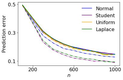
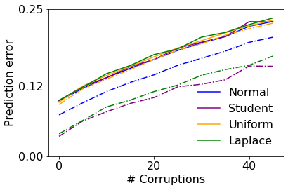
Figure 1: On the left, we plot the prediction error for $|\mathcal{O}|=40$ corruptions, against the number of samples $n$, for various features. On the right, we show for $n=500$ how the prediction error changes as the number of randomly flipped labels $|\mathcal{O}|$ decreases. The solid lines represent the max-$\ell_{1}$-margin estimators $\hat{\beta}$ (2). The dash-dotted lines are instances of AdaBoost $\tilde{\beta}_{T}$, as defined in Algorithm 1.

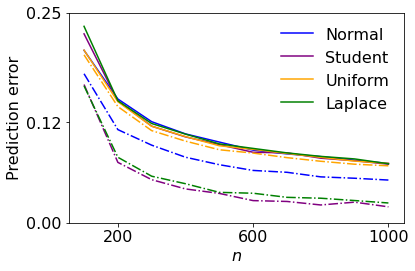
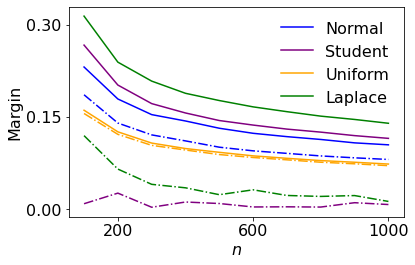
Figure 2: On the left, we consider the same setting as in Figure 2, however in the case of noiseless data $|\mathcal{O}|=0$. On the right, we plot for noiseless data the margins $\gamma$ of the max-$\ell_{1}$-margin estimators, as defined in (1), as well as the $\ell_{1}$-margins of AdaBoost $\tilde{\beta}_{T}$.

The two plots in Figure 2 show the noisy case, while noise is absent in the two plots in Figure 2. For the max-$\ell_{1}$-margin estimator the prediction error for all simulated features appears to behave identically. By contrast, the $\ell_{1}$-margin differs widely across the features by a multiplicative constant, but shows the same asymptotic behaviour.

As stated in Lemma 2.1, we see that the margin of AdaBoost is close to the max $\ell_{1}$-margin and that the performance of AdaBoost is similar to the performance of the max-$\ell_{1}$-margin classifier. The proximity of AdaBoost to its limit appears to depend on the distribution of the features. In particular, the simulations suggest that heavier tails lead to slower convergence. This is reasonable, considering that AdaBoost rescales the features with their $\ell_{\infty}$-norm, see Algorithm 1. This is particularly visible when comparing the uniform distribution, for which the max-$\ell_{1}$-margin estimator and AdaBoost seem to behave almost identically, to the student-t distribution, for which the margin is close to zero for some $n$.

3 Conclusion

In this paper, we have shown that AdaBoost, as described in Algorithm 1, achieves consistent recovery in the presence of small, adversarial errors, despite being overparameterized and interpolating the observations. Our results hold under weak assumptions on the tail behaviour and the behaviour around zero of the feature distribution. In addition, for Gaussian features the derived convergence rates in Corollary 2.3 are comparable to convergence rates of state-of-the-art regularized estimators [46]. This is a first step for the understanding of overparameterized and interpolating AdaBoost and other interpolating algorithms and shows why such algorithms can generalize well in high-dimensional and noisy situations, despite interpolating the data.

However, in the presence of well-behaved noise, as in logistic regression, our bounds are suboptimal and require that the fraction of mislabeled data points decays to zero. By contrast, regularized estimators [46] are able to achieve faster convergence rates in such settings and do not require that the fraction of mislabeled data is asymptotically vanishing to achieve consistency.

Many open question do remain. The convergence rate for Gaussian features in Corollary 2.3 is among the best available results if $\beta^{*}$ is allowed to be genuinely effectively sparse. However, it is not clear whether the exponent in (13) is optimal, and further research about information theoretic lower bounds is needed. When $\beta^{*}$ is exactly sparse, the convergence rate in (13) is sub-optimal and better results for log-concave features have been obtained by [1] for a regularized estimator. Moreover, for noiseless data and exact sparse $\beta^{*}$ our simulations suggest that AdaBoost attains a faster rate than in the noisy case. It thus remains as an interesting further research question how to show that AdaBoost attains faster convergence rates for noiseless data and when $\beta^{*}$ is exact sparse.

Finally, our results rely heavily on the anti-concentration assumption in Definition 2.2, which is not fulfilled for Rademacher features. Assuming additionally $\|\beta^{*}\|_{\infty}=o(1)$ [2] obtained convergence rates for the regularized estimator proposed in [46]. It is straightforward to adapt our lower bound on the max-$\ell_{1}$-margin in Theorem 2.2 to such a setting. However, by contrast, it is not clear how to modify the uniform tesselation result used in the proof of Theorem 2.1 and consequently show convergence rates for AdaBoost without anti-concentration.

4 Proofs

4.1 Proof of Theorem 2.1

Proof.

Let $\tilde{\beta}$ be an approximation of the max $\ell_{1}$-margin. Defining $\bar{\beta}:=2\tilde{\beta}/\left(\gamma_{0}\|\tilde{\beta}\|_{1}\right)$ we have on an event of probability at least $1-t$ that

$$\min_{i\in[n]}y_{i}\langle X_{i},\bar{\beta}\rangle\geq 1,$$

and $\bar{\beta}\in r_{n}B_{1}^{p}$ for $r_{n}=2/\gamma_{0}$. It follows that $\|\tilde{\beta}\|_{1}/\|\tilde{\beta}\|_{2}=\|\bar{\beta}\|_{1}/\|\bar{\beta}\|_{2}$, which we bound by applying the following proposition.

Proposition 4.1.

Assume $p\gtrsim n$ and that $\mathbb{X}=(X_{i})_{i\in[n]}$ has i.i.d. zero mean and unit variance entries and satisfies the weak moment assumption with $\zeta\geq 1/2$. Let $r_{n}>0$ be such that

$$r_{n}\lesssim\sqrt{\frac{n}{\log^{2\zeta+1}(p)\log(n)}}.$$

Then, with probability at least $1-cp^{-1}$ for any $\beta\in\mathbb{R}^{p}$ such that $\|\beta\|_{1}\leq r_{n}$ and $\min_{i\in[n]}y_{i}\langle X_{i},\beta\rangle\geq 1$, we have that

$$\frac{\|\beta\|_{1}}{\|\beta\|_{2}}\lesssim r_{n}.$$

Moreover, assume that $\mathbb{X}$ fulfills a small deviation assumption with parameter $\theta>0$. Then with probability at least $1-cp^{-1}$, for any $\beta\in\mathbb{R}^{p}$ such that $\|\beta\|_{1}\leq r_{n}$ and $\min_{i\in[n]}y_{i}\langle X_{i},\beta\rangle\geq 1$, we have that

$$\frac{\|\beta\|_{1}}{\|\beta\|_{2}}\lesssim\frac{r_{n}}{\tau_{n}},$$

where

$$\tau_{n}\asymp\left[\frac{n}{\log^{2\zeta+1}(p)\log(n)r_{n}^{2}}\right]^{\frac{1}{\theta}}.$$

Having obtained a bound for the ratio $\|\tilde{\beta}\|_{1}/\|\tilde{\beta}\|_{2}$, we next use a sparse hyperplane tesselation result for the pseudo-metric $d$, arguing by contradiction. Since $d$ is scaling invariant, i.e. $d(\beta,\tilde{\beta})=d(\beta,\tilde{\beta}/\|\tilde{\beta}\|_{2})$ it suffices to consider only elements on the unit sphere.

Proposition 4.2.

Assume $p\gtrsim n$ and that $\mathbb{X}=(X_{i})_{i\in[n]}$ has i.i.d. zero mean and unit variance entries and satisfies the weak moment assumption with $\zeta\geq 1/2$ and the anti-concentration assumption with $\alpha\in(0,1]$. For $a>0$, define

$$\eta=c\left(a^{2}\frac{\log^{2\zeta+1}(p)\log(n)}{n}\right)^{\frac{1}{2+\alpha}},$$ (14)

and assume $\eta\leq 1/2$. Define

$$\mathcal{B}(a,\eta)=\left\{\beta\in\mathbb{R}^{p}:~{}d(\beta,\beta^{*})\geq c\eta^{\alpha}\right\}.$$

Then with probability at least $1-cp^{-1}$ we have, uniformly for $\beta\in aB_{1}^{p}\cap\mathcal{S}^{p-1}\cap\mathcal{B}(a,\eta)$

$$\frac{1}{n}\sum_{i=1}^{n}\mathbf{1}\left(\text{sgn}\left(\langle X_{i},\beta\rangle\right)\neq\text{sgn}\left(\langle X_{i},\beta^{*}\rangle\right)\right)\gtrsim\eta^{\alpha}.$$

Now, we apply Proposition 4.6 with $a\asymp r_{n}$. Since $|\mathcal{O}|\lesssim\eta^{\alpha}$ by assumption, we get

$$\frac{1}{n}\sum_{i=1}^{n}\mathbf{1}\left(\text{sgn}\left(\langle X_{i},\tilde{\beta}/\|\tilde{\beta}\|_{2}\rangle\right)\neq\text{sgn}\left(\langle X_{i},\beta^{*}\rangle\right)\right)=\frac{|\mathcal{O}|}{n}\lesssim\eta^{\alpha},$$

and hence, adjusting constants, we have on an event of probability at least $1-t-cp^{-1}$ that $\tilde{\beta}/\|\tilde{\beta}\|_{2}\notin\mathcal{B}(a,\eta)$ and hence on the same event $d(\tilde{\beta},\beta^{*})\lesssim\eta^{\alpha}$.

When $\mathbb{X}$ satisfies the small deviation assumption with parameter $\theta>0$, we apply Proposition 4.6 with $a\asymp r_{n}/\tau_{n}$. Since $|\mathcal{O}|\lesssim\eta^{\alpha\left(1+\frac{2}{\theta}\right)}$ by assumption, we conclude the proof using the same reasoning. ∎

4.2 Upper and lower bounds for the max $\ell_{1}$-margin

4.2.1 Proof of Theorem 2.2

We start this section with the following lemma. A proof is given in [38].

Lemma 4.1 (Proposition A.2 in [38]).

Suppose that

$$\gamma:=\max_{\beta\neq 0}\min_{1\leq i\leq n}\frac{y_{i}\langle X_{i},\beta\rangle}{\|\beta\|_{1}}>0.$$

Then, we have that $\gamma^{-1}=\|\hat{\beta}\|_{1}$, where

$$\hat{\beta}\in\operatorname*{arg\,min}_{\beta\in\mathbb{R}^{p}}\left\{\|\beta\|_{1}\quad\textnormal{subject to}\quad y_{i}\langle X_{i},\beta\rangle\geq 1\right\}.$$ (15)

Hence, in order to lower bound $\gamma$ it suffices to upper bound $\|\hat{\beta}\|_{1}$, which is accomplished in the following proposition.

Proposition 4.3.

Assume $p\gtrsim n$ and that $\mathbb{X}=(X_{i})_{i\in[n]}$ has i.i.d. symmetric, zero mean and unit variance entries and satisfies the weak moment assumption with $\zeta\geq 1/2$ and the anti-concentration assumption with $\alpha\in(0,1]$. Then with probability at least $1-cn^{-2}$ we have that

$$\|\hat{\beta}\|_{1}\lesssim\left[\frac{n}{\log(ep/n)}\left(s+\frac{\log^{1+2\zeta}(n)|\mathcal{O}|}{\log(ep/n)}+\log^{1+2\zeta}(n)\right)^{\alpha/2}\right]^{1/(2+\alpha)}.$$ (16)

Proof.

We prove Proposition 4.3 by explicitly constructing a $\beta$ that fulfills the constraints in (15). For $\varepsilon>0$, we define a lifting function $f_{\varepsilon}:\mathbb{R}\rightarrow\mathbb{R}$

$$f_{\varepsilon}(x):=\left\{\begin{array}[]{ll}x-\varepsilon&\mbox{if }0\leq x\leq\varepsilon\\ x+\varepsilon&\mbox{if }-\varepsilon\leq x<0\\ 0&\mbox{otherwise. }\end{array}\right.$$

For $i\in[n]$, we denote

$$z_{i}=\begin{cases}&f_{\varepsilon}\big{(}\langle X_{i},\beta^{*}\rangle)~{}~{}~{}~{}~{}~{}~{}~{}~{}~{}~{}~{}~{}~{}~{}~{}~{}~{}~{}i\notin\mathcal{O}\\ &2\langle X_{i},\beta^{*}\rangle-f_{\varepsilon}\big{(}\langle X_{i},\beta^{*}\rangle)~{}~{}~{}i\in\mathcal{O}\\ \end{cases}$$

and $Z=(z_{1},\cdots,z_{n})^{T}$. Finally, we define

$$\hat{\nu}\in\operatorname*{arg\,min}_{\beta\in\mathbb{R}^{p}}\|\beta\|_{1}\quad\text{subject to}~{}~{}\langle X_{i},\beta\rangle=z_{i},~{}~{}~{}i=1,\dots,n.$$ (17)

By definition of $\hat{\nu}$, if $i\in\mathcal{O}$, we have the decomposition

$$\langle X_{i},\beta^{*}-\hat{\nu}\rangle =-\langle X_{i},\beta^{*}\rangle+f_{\varepsilon}\big{(}\langle X_{i},\beta^{*}\rangle\big{)}$$

$$=\left\{\begin{array}[]{ll}-\langle X_{i},\beta^{*}\rangle&\mbox{if }|\langle X_{i},\beta\rangle^{*}|\geq\varepsilon\\ -\varepsilon&\mbox{if }0\leq\langle X_{i},\beta^{*}\rangle\leq\varepsilon\\ \varepsilon&\mbox{if }-\varepsilon\leq\langle X_{i},\beta^{*}\rangle<0.\end{array}\right.$$

A similar decomposition with each equation above multiplied with $-1$ holds if $i\notin\mathcal{O}$. Hence, we have that $\text{sgn}\left(\langle X_{i},\beta^{*}-\hat{\nu}\rangle\right)=y_{i}$ and $|\langle X_{i},\beta^{*}-\hat{\nu}\rangle|\geq\varepsilon$ for $i=1,\dots,n$. It follows that

$$\|\hat{\beta}\|_{1}\leq\frac{\|\beta^{*}-\hat{\nu}\|_{1}}{\varepsilon}\leq\frac{\sqrt{s}}{\varepsilon}+\frac{\|\hat{\nu}\|_{1}}{\varepsilon}.$$

We now apply Proposition B.1 and obtain that with probability at least $1-2\exp(-2n)$

$$\|\hat{\nu}\|_{1}\lesssim\frac{\|Z\|_{2}}{\sqrt{\log(ep/n)}}+\|Z\|_{\infty}.$$

By Lemma B.1 we have with probability at least $1-n^{-2}$ that

$$\|Z\|_{\infty}\leq\varepsilon+\max_{i\in[n]}|\langle X_{i},\beta^{*}\rangle|\lesssim\varepsilon+\log^{1/2+\zeta}(n).$$

It is left to bound $\|Z\|_{2}$. By the triangle inequality, we have that

$$\|Z\|_{2}\leq 2\sqrt{\sum_{i\in\mathcal{O}}|\langle X_{i},\beta^{*}\rangle|^{2}}+\sqrt{\sum_{i=1}^{n}f_{\varepsilon}(\langle X_{i},\beta^{*}\rangle)^{2}}.$$ (18)

By Lemma B.1 we have with probability at least $1-n^{-2}$

$$\sum_{i\in\mathcal{O}}|\langle X_{i},\beta^{*}\rangle|^{2}\leq|\mathcal{O}|\max_{i\in[n]}|\langle X_{i},\beta^{*}\rangle|^{2}\lesssim|\mathcal{O}|\log^{1+2\zeta}(n).$$

We next bound the second term on the right hand side in (18). Indeed, we have that

$$\frac{1}{n}\sum_{i=1}^{n}f_{\varepsilon}(\langle X_{i},\beta^{*}\rangle)^{2} =\frac{1}{n}\sum_{i=1}^{n}(|\langle X_{i},\beta^{*}\rangle|-\varepsilon)^{2}\mathbf{1}(|\langle X_{i},\beta^{*}\rangle|\leq\varepsilon)$$

$$\leq\frac{\varepsilon^{2}}{n}\sum_{i=1}^{n}\mathbf{1}(|\langle X_{i},\beta^{*}\rangle|\leq\varepsilon)$$ (19)

Let $p_{\varepsilon}=\mathbb{P}(|\langle X_{1},\beta^{*}\rangle|\leq\varepsilon)$. By Hoeffding’s inequality, Theorem 3.1.2 in [28], we have with probability at least $1-\exp(-2n\varepsilon^{2\alpha})$ that

$$\frac{1}{n}\sum_{i=1}^{n}f_{\varepsilon}(\langle X_{i},\beta^{*}\rangle)^{2}\leq\frac{\varepsilon^{2}}{n}\sum_{i=1}^{n}\mathbf{1}(|\langle X_{i},\beta^{*}\rangle|\leq\varepsilon)\leq\varepsilon^{2}\left(p_{\varepsilon}+\varepsilon^{\alpha}\right)\lesssim\varepsilon^{2+\alpha},$$

where the last inequality holds by the anti-concentration assumption and for $p^{-1}\leq\varepsilon\leq 1$. Hence, summarizing, we have with probability at least $1-e^{-2n\varepsilon^{2\alpha}}-n^{-2}-2\exp(-2n)$ that

$$\|\hat{\nu}\|_{1}\lesssim\frac{\log^{1/2+\zeta}(n)|\mathcal{O}|^{1/2}+n^{1/2}\varepsilon^{1+\alpha/2}}{\sqrt{\log(ep/n)}}+\varepsilon+\log(n)^{1/2+\zeta}$$

Choosing

$$\varepsilon\asymp\left(\frac{s\log(ep/n)}{n}+\frac{|\mathcal{O}|\log(n)^{1+2\zeta}}{n}\right)^{\frac{1}{2+\alpha}}$$

concludes the proof. ∎

4.2.2 Proof of Proposition 2.1

Proof.

By the dual formulation of the margin (see Appendix A), we have that

$$\gamma=\inf_{w:~{}w_{i}\geq 0~{}\forall i\in[n],\|w\|_{1}=1}\left\|\sum_{i=1}^{n}w_{i}y_{i}X_{i}\right\|_{\infty}.$$ (20)

Hence, for proving an upper bound it suffices to find an appropriate weighting $w$. For $\tau_{n}$ a sequence to be defined and $\tau_{n}^{-1}$ taking integer values, we define

$$w_{i}=\begin{cases}&\tau_{n}~{}~{}~{}~{}~{}i~{}\text{is among indices of}~{}\tau_{n}^{-1}~{}\text{smallest entries of}(|\langle X_{i},\beta^{*}\rangle|)_{i=1}^{n}\\ &0~{}~{}~{}~{}~{}~{}\text{otherwise}.\end{cases}$$

We use this choice of $w$ to upper bound $\gamma$. We denote the projector onto the space spanned by $\beta^{*}$ by $P$, $P:=\beta^{*}(\beta^{*})^{T}$, and define its orthogonal complement $P^{\perp}:=I_{p}-P$. We have that

$$\left\|\sum_{i=1}^{n}w_{i}y_{i}X_{i}\right\|_{\infty}\leq\left\|\sum_{i=1}^{n}w_{i}y_{i}PX_{i}\right\|_{\infty}+\left\|\sum_{i=1}^{n}w_{i}y_{i}P^{\perp}X_{i}\right\|_{\infty}.$$ (21)

We treat the two terms separately. For the first term, we have by Theorem 5 and Theorem 7 in [27] that

$$\mathbb{E}\left\|\sum_{i=1}^{n}w_{i}y_{i}PX_{i}\right\|_{\infty} =\mathbb{E}\left\|\sum_{i=1}^{n}w_{i}|\langle X_{i},\beta^{*}\rangle|\beta^{*}\right\|_{\infty}=\left\|\beta^{*}\right\|_{\infty}\mathbb{E}\sum_{i=1}^{n}w_{i}|\langle X_{i},\beta^{*}\rangle|$$

$$\lesssim\|\beta^{*}\|_{\infty}\sum_{k=1}^{\tau_{n}^{-1}}\frac{\tau_{n}k\log(k+1)}{n}\lesssim\frac{\|\beta^{*}\|_{\infty}(\tau_{n}^{-1}+1)\log(p)}{n}.$$

We next bound the second term on the right hand side in (21). Observe that $y_{i}=\text{sgn}(\langle X_{i},\beta^{*}\rangle)=\text{sgn}(\langle PX_{i},\beta^{*}\rangle)$ and hence $y_{i}$ is independent of $P^{\perp}X_{i}$. Likewise, $w$ is a function of $(PX_{i})_{i}$ and not $(P^{\perp}X_{i})_{i}$ and hence $w$ and $P^{\perp}X_{i}$ are independent for each $i$. We conclude that

$$\left(\sum_{i}w_{i}y_{i}P^{\perp}X_{i}\right)_{j}\thicksim\mathcal{N}(0,\|w\|_{2}^{2}\langle e_{j},P^{\perp}e_{j}\rangle).$$

Hence, using a standard Chernoff-bound, we obtain

$$\mathbb{E}\left\|\sum_{i}w_{i}y_{i}PX_{i}\right\|_{\infty} \lesssim\sqrt{\log(p)\|w\|_{2}^{2}}=\sqrt{\log(p)\tau_{n}}.$$

Hence, we obtain

$$\mathbb{E}\gamma\leq\mathbb{E}\left\|\sum_{i=1}^{n}w_{i}y_{i}X_{i}\right\|_{\infty}\lesssim\frac{\|\beta^{*}\|_{\infty}\log(p)}{n\tau_{n}}+\sqrt{\log(p)\tau_{n}}.$$

The final result is obtained by choosing

$$\tau_{n}^{-1}=\left\lceil\left(\frac{n}{\|\beta^{*}\|_{\infty}\log(p)}\right)^{2/3}\right\rceil.$$

∎

4.3 Proof Proposition 4.1

4.3.1 Proof of the first part of Proposition 4.1

In this subsection, we present a result holding only under the weak moment assumption. We will see in the next section how to improve this result when assuming a small deviation assumption.

Proposition 4.4.

Assume that $\mathbb{X}=(X_{i})_{i\in[n]}$ has i.i.d. zero mean and unit variance entries and satisfies the weak moment assumption with $\zeta\geq 1/2$. Suppose that $r_{n}>0$ satisfies

$$r_{n}\lesssim\sqrt{\frac{n}{\log(p)}}.$$

Then, with probability at least

$$1-np^{-2}-2\exp\left(-\frac{cn}{r_{n}^{2}\log^{2\zeta}(p)}\right),$$

for any $\beta\in\mathbb{R}^{p}$ such that $\|\beta\|_{1}\leq r_{n}$ and $\min_{i\in[n]}y_{i}\langle X_{i},\beta\rangle\geq 1$, we have that $\|\beta\|_{2}\geq 1/2$.

Proof.

For $r_{n}>0$, let $\beta\in\mathbb{R}^{p}$ such that $\|\beta\|_{1}\leq r_{n}$ and $\min_{i\in[n]}y_{i}\langle X_{i},\beta\rangle\geq 1$. Thus, we have

$$\frac{1}{n}\sum_{i=1}^{n}|\langle X_{i},\beta\rangle|\geq 1.$$ (22)

We proceed by contradiction. Assume that $\|\beta\|_{2}\leq 1/2$. In this case, we show that Equation (22) is not satisfied with large probability, concluding the proof by contradiction.
For $i\in[n]$, using Hölder’s inequality, we have that

$$|\langle X_{i},\beta\rangle|\leq\|X_{i}\|_{\infty}\|\beta\|_{1}\leq r_{n}\|X_{i}\|_{\infty}\lesssim r_{n}\log^{\zeta}(p),$$

where the last inequality follows from Lemma B.1 and holds with probability at least $1-p^{-2}$. Thus, with probability at least $1-n/p^{2}$ we have, for all $i\in[n]$, that $|\langle X_{i},\beta\rangle|\lesssim r_{n}\log^{\zeta}(p)$. Hence, conditioning on this event and using the bounded differences inequality, Theorem 3.3.14 in [28], we obtain with probability at least

$$1-2\exp\left(-\frac{cn}{r_{n}^{2}\log^{2\zeta}(p)}\right)-n/p^{2}$$

that we have

$$\sup_{\beta\in r_{n}B_{1}^{p}\cap(1/2)B_{2}^{p}}\frac{1}{n}\sum_{i=1}^{n}|\langle X_{i},\beta\rangle| \leq\sup_{\beta\in r_{n}B_{1}^{p}\cap(1/2)B_{2}^{p}}\mathbb{E}|\langle X_{1},\beta\rangle|$$

$$+\mathbb{E}\sup_{\beta\in r_{n}B_{1}^{p}\cap(1/2)B_{2}^{p}}\frac{1}{n}\sum_{i=1}^{n}|\langle X_{i},\beta\rangle|-\mathbb{E}|\langle X_{i},\beta\rangle|+\frac{1}{4}.$$

By Jensen’s inequality and the fact $X$ is isotropic with unit variance, we obtain that

$$\sup_{\beta\in r_{n}B_{1}^{p}\cap(1/2)B_{2}^{p}}\mathbb{E}|\langle X_{1},\beta\rangle|\leq 1/2.$$

Moreover, we have that

$$\mathbb{E}\sup_{\beta\in r_{n}B_{1}^{p}\cap(1/2)B_{2}^{p}}\frac{1}{n}\sum_{i=1}^{n}|\langle X_{i},\beta\rangle|-\mathbb{E}|\langle X_{i},\beta\rangle| \leq\mathbb{E}\sup_{\beta\in r_{n}B_{1}^{p}\cap(1/2)B_{2}^{p}}\frac{4}{n}\sum_{i=1}^{n}\sigma_{i}\langle X_{i},\beta\rangle$$

$$\lesssim r_{n}\sqrt{\frac{\log(p)}{n}},$$

where $(\sigma_{i})_{i=1}^{n}$ are i.i.d Rademacher random variables independent from $(X_{i})_{i=1}^{n}$. We used in the first line the symmetrization and contraction principles, Theorem 3.1.21 and Theorem 3.2.1. in [28] and Proposition B.2 in the second line to bound the Rademacher complexity.
The condition on $r_{n}$ shows that

$$\sup_{\beta\in r_{n}B_{1}^{p}\cap(1/2)B_{2}^{p}}\frac{1}{n}\sum_{i=1}^{n}|\langle X_{i},\beta\rangle|<1,$$

and the contradiction is established.

∎

4.3.2 Proof of the second part of Proposition 4.1: small deviation assumption

In this subsection, we show how to prove the second part of Proposition 4.1 under the small deviation assumption 2.3.

Proposition 4.5.

Assume $p\gtrsim n$ and that $\mathbb{X}=(X_{i})_{i\in[n]}$ has i.i.d. zero mean and unit variance entries and satisfies the weak moment assumption with $\zeta\geq 1/2$. Moreover, assume that $\mathbb{X}$ fulfills a small deviation assumption, Definition 2.3, with constant $\theta>0$. Let $r_{n}\geq 1$, define

$$\tau_{n}=c\left(\frac{n}{\log^{2\zeta+1}(p)\log(n)r_{n}^{2}}\right)^{\frac{1}{\theta}}$$

and suppose that $\tau_{n}\gtrsim 1$. Then, with probability at least $1-p^{-1}$ for any $\beta\in\mathbb{R}^{p}$ such that $\|\beta\|_{1}\leq r_{n}$ and $\min_{i\in[n]}y_{i}\langle X_{i},\beta\rangle\geq 1$, we have that $\|\beta\|_{1}/\|\beta\|_{2}\lesssim r_{n}/\tau_{n}$.

Proof of Proposition 4.5. Let $\{{\rm e}_{j}\}_{j=1}^{p}$ be the set of standard unit vectors in $\mathbb{R}^{p}$ and ${\cal D}:=\{\pm e_{j}\}\cup\{0\}\subset\mathbb{R}^{p}$ be the set of vectors with all entries equal to zero possibly except just one, where the value is then $\pm 1$. We define, for $m\in\mathbb{N}$, Maurey’s set

$${\cal Z}_{m}:=\biggl{\{}z={1\over m}\sum_{k=1}^{m}z_{k},\ z_{k}\in{\cal D}\ \forall\ k\biggr{\}}.$$

Take

$$m=c\log^{2\zeta}(p)\log(n)r_{n}^{2},$$

and define the event

$${\cal E}_{\rm max}:=\{\|\mathbb{X}\|_{\infty}\leq c\log^{\zeta}(p)\},$$

and observe that by Lemma B.1, the event ${\cal E}_{\rm max}$ occurs with probability at least $1-p^{-1}$ as $p\gtrsim n$. Then, by Lemma 4.2, for all $\beta\in r_{n}B_{1}^{p}$ such that $\|\beta\|_{2}\lesssim\tau_{n}$ there exists a vector $z_{\beta}\in r_{n}{\cal Z}_{m}$ such that on ${\cal E}_{\rm max}$

$$\max_{1\leq i\leq n}|\langle X_{i},\beta\rangle-\langle X_{i},z_{\beta}\rangle|\lesssim\log^{\zeta}(p)r_{n}\sqrt{\log(2n)\over m}\leq{1\over 2}$$

as well as $\|\beta-z_{\beta}\|_{2}\leq 1/2$, for $m$ defined previously. Thus, we also have by assumption on $\tau_{n}$

$$\|z_{\beta}\|_{2}\lesssim\tau_{n}+1/2\lesssim\tau_{n}.$$

In other words, on ${\cal E}_{\rm max}$ we have that $\{z_{\beta}:\|\beta\|_{1}\leq r_{n},\|\beta\|_{2}\leq c\tau_{n}\}\subset r_{n}{\cal Z}_{m}\cap\{\beta:\|\beta\|_{2}\leq c\tau_{n}\}=:{\cal Z}_{m}(r_{n},\tau_{n})$. We invoke that

$$\biggl{\{}\sup_{\beta\in r_{n}B_{1}^{p}\cap\{\beta:\|\beta\|_{2}\lesssim\tau_{n}\}}\min_{1\leq i\leq n}|\langle X_{i},\beta\rangle|\geq 1\biggr{\}}\cap{\cal E}_{\rm max}$$

$$\subseteq \biggl{\{}\max_{z\in{\cal Z}_{m}(r_{n},\tau_{n})}\min_{1\leq i\leq n}|\langle X_{i},z\rangle|\geq{1\over 2}\biggr{\}}.$$

For all $z\in{\cal Z}_{m}(r_{n},\tau_{n})$ and $i\in[n]$ by the small deviation assumption 2.3, we have

$$\mathbb{P}\biggl{(}|\langle X_{i},z\rangle|\leq{1\over 2}\biggr{)}\geq\mathbb{P}\biggl{(}{|\langle X_{i},z\rangle|\over\|z\|_{2}}\leq{c\over\tau_{n}}\biggr{)}\gtrsim\tau_{n}^{-\theta}.$$

Hence,

$$\mathbb{P}\biggl{(}|\langle X_{i},z\rangle|\geq{1\over 2}\biggr{)}\leq\biggl{(}1-c\tau_{n}^{-\theta}\biggr{)}\leq\exp\biggl{[}-c\tau_{n}^{-\theta}\biggr{]}$$

and thus we obtain

$$\mathbb{P}\biggl{(}\min_{1\leq i\leq n}|\langle X_{i},z\rangle|\geq{1\over 2}\biggr{)}\leq\exp\biggl{[}-cn\tau_{n}^{-\theta}\biggr{]}.$$

Since

$$|{\cal Z}_{m}(r_{n},\tau_{n})|\leq|{\cal Z}_{m}|\leq(2p+1)^{m}.$$

we obtain by a union bound that

$$\mathbb{P}\biggl{(}\max_{z\in{\cal Z}_{m}(r_{n},\tau_{n})}\min_{1\leq i\leq n}|\langle X_{i},z\rangle|\geq{1\over 2}\biggr{)}\leq\exp\biggl{[}m\log(2p+1)-cn\tau_{n}^{-\theta}\biggr{]}.$$

We conclude that

$$\mathbb{P}\biggl{(}\sup_{\beta\in r_{n}B_{1}^{p}\cap\{\beta:\|\beta\|_{2}\leq c\tau_{n}\}}\min_{1\leq i\leq n}|\langle X_{i},\beta\rangle|\geq 1\biggr{)} \leq\exp\biggl{[}m\log(2p+1)-cn\tau_{n}^{-\theta}\biggr{]}+\mathbb{P}({\cal E}_{\rm max}^{c})$$

$$\leq\exp\left(-cn\tau_{n}^{-\theta}\right)+p^{-1},$$

from our choice of $m$ and applying Lemma B.1.

4.4 Tesselation

Proposition 4.6.

Assume $p\gtrsim n$ and that $\mathbb{X}=(X_{i})_{i\in[n]}$ has i.i.d. zero mean and unit variance entries and satisfies the weak moment assumption with $\zeta\geq 1/2$ and the anti-concentration assumption with $\alpha\in(0,1]$. For $a>0$ define

$$\eta=c\left(\frac{a^{2}\log^{2\zeta+1}(p)\log(n)}{n}\right)^{\frac{1}{2+\alpha}},$$ (23)

and assume $\eta\lesssim 1$. Define

$$\mathcal{B}(a,\eta)=\left\{\beta\in\mathbb{R}^{p}:d(\beta,\beta^{*})\geq c\eta^{\alpha}\right\}.$$

Then with probability at least

$$1-2\exp\left(-cn\eta^{\alpha}\right)-np^{-2}$$

we have, uniformly for $\beta\in aB_{1}^{p}\cap\mathcal{S}^{p-1}\cap\mathcal{B}(a,\eta)$

$$\frac{1}{n}\sum_{i=1}^{n}\mathbf{1}\{\text{sgn}\left(\langle X_{i},\beta\rangle\right)\neq\text{sgn}\left(\langle X_{i},\beta^{*}\rangle\right)\}\gtrsim\eta^{\alpha}.$$

Proof.

For $a>0$ and $\eta$ defined in Equation (23) let $\beta\in aB_{1}^{p}\cap\mathcal{S}^{p-1}\cap\mathcal{B}(a,\eta)$. By Lemma 4.2 there exists $z_{\beta}$ in $\mathcal{Z}_{m}$ such that

$$\max_{i\in[n]}|\langle X_{i},\beta-z_{\beta}\rangle|{\rm l}_{{\cal E}_{\rm max}}\lesssim a\log^{\zeta}(p)\sqrt{\frac{\log(n)}{m}}\asymp\eta~{}~{}\text{and}~{}~{}\|\beta-z_{\beta}\|_{2}\lesssim\frac{1}{\sqrt{m}}$$

where ${\cal E}_{\rm max}:=\{\|\mathbb{X}\|_{\infty}\leq c\log^{\zeta}(p)\}$ and for $m=ca^{2}\log^{2\zeta}(p)\log(n)/\eta^{2}$. We note that by Lemma B.1 ${\cal E}_{\rm max}$ occurs with probability at least $1-np^{-2}$. In particular we have $1/2\leq 1-\eta\leq\|z_{\beta}\|_{2}\leq 1+\eta\leq 3/2$, for $\eta$ small enough. Let $z_{\beta}\in\mathcal{Z}_{m}$. By Bernstein’s inequality, Theorem 3.1.7 in [28], and the anti-concentration assumption, we have that

$$\sum_{i=1}^{n}\mathbf{1}\{|\langle X_{i},z_{\beta}\rangle|\leq\eta\} \leq n\left(\mathbb{P}\left(|\langle X_{1},z_{\beta}\rangle|\leq\eta\right)+\eta^{\alpha}\right)$$

$$\leq n\left(\mathbb{P}\left(|\langle X_{1},\frac{z_{\beta}}{\|z_{\beta}\|_{2}}\rangle|\leq 2\eta\right)+\eta^{\alpha}\right)$$

$$\leq n\left(\sup_{\beta\in\mathcal{S}^{p-1}}\mathbb{P}\left(\langle X_{1},\beta\rangle|\leq 2\eta\right)+\eta^{\alpha}\right)$$

$$\lesssim n\eta^{\alpha}$$

with probability at least $1-\exp(-cn\eta^{\alpha})$. Now, define

$$J:=\left\{i\in[n]:\min_{z_{\beta}\in\mathcal{Z}_{m}}|\langle X_{i},z_{\beta}\rangle|\geq\eta\right\}.$$

Using an bound over $\mathcal{Z}_{m}$ and that $|\mathcal{Z}_{m}|\leq(2p+1)^{m}$, we obtain that with probability at least

$$1-2\exp\left[m\log(2p+1)-cn\eta^{\alpha}\right]\geq 1-2\exp[-cn\eta^{\alpha}]$$

we have uniformly for $z_{\beta}\in\mathcal{Z}_{m}$

$$|J^{C}|\lesssim\eta^{\alpha}n.$$

For $i\in J$ and working on the event ${\cal E}_{\rm max}$ we have that $|\langle X_{i},z_{\beta}\rangle|\geq\eta$ and $|\langle X_{i},\beta-z_{\beta}\rangle|<\eta$ and hence $\langle X_{i},\beta\rangle$ and $\langle X_{i},z_{\beta}\rangle$ have matching signs.

Hence, for $\beta\in aB_{1}^{p}\cap\mathcal{S}^{p-1}\cap\mathcal{B}(a,\eta)$ and working on the event ${\cal E}_{\rm max}$, we have

$$\sum_{i=1}^{n}\mathbf{1}\{\text{sgn}\left(\langle X_{i},\beta\rangle\right)\neq\text{sgn}\left(\langle X_{i},\beta^{*}\rangle\right)\} \geq\sum_{i\in J}\mathbf{1}\{\text{sgn}\left(\langle X_{i},\beta\rangle\right)\neq\text{sgn}\left(\langle X_{i},\beta^{*}\rangle\right)\}$$

$$=\sum_{i\in J}\mathbf{1}\{\text{sgn}\left(\langle X_{i},z_{\beta}\rangle\right)\neq\text{sgn}\left(\langle X_{i},\beta^{*}\rangle\right)\}$$

$$\geq\sum_{i=1}^{n}\left(\mathbf{1}\{\text{sgn}\left(\langle X_{i},z_{\beta}\rangle\right)\neq\text{sgn}\left(\langle X_{i},\beta^{*}\rangle\right)-c\eta^{\alpha}\right).$$

Applying Bernstein’s inequality, Theorem 3.1.7 in [28] we have that

$$\sum_{i=1}^{n}\mathbf{1}\left(\text{sgn}\left(\langle X_{i},z_{\beta}\rangle\right)\neq\text{sgn}\left(\langle X_{i},\beta^{*}\rangle\right)\right)\geq \bigg{(}d(z_{\beta},\beta^{*})-c\eta^{\alpha}\bigg{)}n$$

with probability at least $1-\exp\left(-cn\eta^{\alpha}\right)$. We next lower bound $d(z_{\beta},\beta^{*})$. Indeed, arguing as above, we have that

$$d(z_{\beta},\beta^{*})=\mathbb{P}\left(\text{sgn}\left(\langle X,z_{\beta}\rangle\right)\neq\text{sgn}\left(\langle X,\beta^{*}\rangle\right)|(y_{i},X_{i})_{i=1}^{n}\right)$$

$$\geq\mathbb{P}\left(\text{sgn}\left(\langle X,z_{\beta}\rangle\right)\neq\text{sgn}\left(\langle X,\beta^{*}\rangle\right),~{}|\langle X,z_{\beta}\rangle|\geq\eta,~{}|\langle X,z_{\beta}-\beta\rangle|<\eta|(y_{i},X_{i})_{i=1}^{n}\right)$$

$$=\mathbb{P}\left(\text{sgn}\left(\langle X,\beta\rangle\right)\neq\text{sgn}\left(\langle X,\beta^{*}\rangle\right),~{}|\langle X,z_{\beta}\rangle|\geq\eta,~{}|\langle X,z_{\beta}-\beta\rangle|<\eta|(y_{i},X_{i})_{i=1}^{n}\right)$$

$$\geq d(\beta,\beta^{*})-\mathbb{P}\left(|\langle X,z_{\beta}\rangle|\leq\eta|(y_{i},X_{i})_{i=1}^{n}\right)-\mathbb{P}\left(|\langle X,z_{\beta}-\beta\rangle|\geq\eta|(y_{i},X_{i})_{i=1}^{n}\right).$$

Since $d(\beta,\beta^{*})\gtrsim\eta^{\alpha}$, $\mathbb{P}\left(|\langle X,z_{\beta}\rangle|\leq\eta|(y_{i},X_{i})_{i=1}^{n}\right)\lesssim\eta^{\alpha}$ by the anti-concentration assumption (Definition 2.2) and $\mathbb{P}\left(|\langle X,z_{\beta}-\beta\rangle|>\eta|(y_{i},X_{i})_{i=1}^{n}\right)\lesssim n^{-2}\lesssim\eta^{\alpha}$ by our choice of $m$ and Lemma B.1, we obtain when the constant in the definition of $\mathcal{B}(a,\eta)$ is large enough that

$$d(z_{\beta},\beta^{*})\gtrsim\eta^{\alpha}.$$

Hence, taking another union bound over $\mathcal{Z}_{m}$ and ${\cal E}_{\rm max}$ and for the constant in the definition of $\mathcal{B}(a,\eta)$ large enough, we obtain with probability at least

$$1-2\exp\left[m\log(2p+1)-c\eta^{\alpha}n\right]-np^{-2}\geq 1-2\exp[-c\eta^{\alpha}n]-np^{-2}$$

that uniformly for $\beta\in aB_{1}^{p}\cap\mathcal{S}^{p-1}\cap\mathcal{B}(a,\eta)$

$$\sum_{i=1}^{n}\mathbf{1}\left(\text{sgn}\left(\langle X_{i},\beta\rangle\right)\neq\text{sgn}\left(\langle X_{i},\beta^{*}\rangle\right)\right)\gtrsim\eta^{\alpha}n$$

which concludes the proof.

∎

4.5 Rest of the proofs

4.5.1 Lemma 4.2

The following Lemma applies Maurey’s empirical method [13, 15] to construct a set $\mathcal{Z}_{m}$ that approximates the $B_{1}^{p}$-ball well.

Lemma 4.2.

(Maurey’s Lemma) Let $\{{\rm e}_{j}\}_{j=1}^{p}$ be the set of standard unit vectors in $\mathbb{R}^{p}$ and ${\cal D}:=\{\pm e_{j}\}\cup\{0\}\subset\mathbb{R}^{p}$ be the set of vectors with all entries equal to zero except at most one, where the value is then $\pm 1$. Define, for $m\in\mathbb{N}$, Maurey’s set

$${\cal Z}_{m}:=\biggl{\{}z={1\over m}\sum_{k=1}^{m}z_{k},\ z_{k}\in{\cal D}\ \forall\ k\biggr{\}}.$$

Then, we have that ${\cal Z}_{m}\subset B_{1}^{p}$ and that $|{\cal Z}_{m}|\leq(2p+1)^{m}$. Moreover, for every $\beta\in B_{1}^{p}$ there exists a vector $z_{\beta}\in{\cal Z}_{m}$ such that for ${\cal E}_{\rm max}:=\{\|\mathbb{X}\|_{\infty}\leq c\log^{\zeta}(p)\}$ we have that

$$\max_{1\leq i\leq n}|\langle X_{i},\beta\rangle-\langle X_{i},z_{\beta}\rangle|{\rm l}_{{\cal E}_{\rm max}}\lesssim\log^{\zeta}(p)\sqrt{\log(n)\over m}~{}~{}~{}~{}\text{and}~{}~{}~{}~{}\|\beta-z_{\beta}\|_{2}\lesssim\frac{1}{\sqrt{m}}.$$

Proof.

For $z\in{\cal D}$ either $\|z\|_{1}=1$ or $z\equiv 0$. Thus for $\bar{z}:=\sum_{k=1}^{m}z_{k}/m\in{\cal Z}_{m}$ we have $\|\bar{z}\|_{1}\leq\sum_{k=1}^{m}\|z_{k}\|_{1}/m\leq 1$. It is moreover clear that $|{\cal D}|=(2p+1)$. Therefore $|{\cal Z}_{m}|\leq(2p+1)^{m}$.

We now turn to the main part of the lemma. Let $\beta\in B_{1}^{p}$. Define a random vector $Z\in{\cal D}$ by

$$\mathbb{P}\biggl{(}Z={\rm sign}(\beta_{j}){\rm e}_{j}\biggr{)}=|\beta_{j}|,\ {\rm for}\ \beta_{j}\not=0,\ j=1,\ldots,p,$$

and

$$\mathbb{P}\biggl{(}Z=0\biggr{)}=1-\|\beta\|_{1}.$$

Then

$$\mathbb{E}Z=\beta,\ \mathbb{E}\|\beta-Z\|_{2}^{2}=\|\beta\|_{1}-\|\beta\|_{2}^{2}\leq\|\beta\|_{1}\leq 1.$$

Let $Z_{1},\ldots,Z_{m}$ be independent copies of $Z$ and define $\bar{Z}:=\sum_{k=1}^{m}Z_{k}/m$. Then we get

$$\mathbb{E}\|\beta-\bar{Z}\|_{2}^{2}\leq{1\over m}.$$

Let $\sigma_{1},\ldots\sigma_{m}$ be a Rademacher sequence independent of ($\mathbb{X},(Z_{1},\ldots,Z_{m}))$. Then we have by the symmetrization inequality, Theorem 3.1.21 in [28], that

$$\mathbb{E}\biggl{[}\max_{1\leq i\leq n}|\langle X_{i},\beta\rangle-\langle X_{i},\bar{Z}\rangle|\ \biggr{|}\mathbb{X}\biggr{]}\leq{2\over m}\mathbb{E}\biggl{[}\max_{1\leq i\leq n}|\sum_{k=1}^{m}\sigma_{k}\langle X_{i},\bar{Z}_{k}\rangle|\ \biggr{|}\ \mathbb{X}\biggr{]}.$$

Further, for $i=1,\ldots,n$, we have that

$$\sum_{k=1}^{m}\langle X_{i},Z_{k}\rangle^{2}\leq m\|X_{i}\|_{\infty}^{2}\leq m\|\mathbb{X}\|_{\infty}^{2}.$$

Thus we obtain,

$$\mathbb{E}\biggl{[}\max_{1\leq i\leq n}|\sum_{k=1}^{m}\sigma_{k}\langle X_{i},Z_{k}\rangle|\ \biggr{|}\ \mathbb{X},\ Z_{1},\ldots,Z_{m}\biggr{]}\leq\sqrt{2\log(2n)}\sqrt{m}\|\mathbb{X}\|_{\infty}.$$

Hence, and since

$${\cal E}_{\rm max}=\biggl{\{}\|\mathbb{X}\|_{\infty}\leq c\log^{\zeta}(p)\biggr{\}},$$

we obtain that

$$\mathbb{E}\biggl{[}\max_{1\leq i\leq n}|\langle X_{i},\beta\rangle-\langle X_{i},\bar{Z}\rangle|{\rm l}_{{\cal E}_{\rm max}}\biggr{]}\lesssim\log^{\zeta}(p)\sqrt{\frac{\log(n)}{m}}.$$

Invoking Jensen’s inequality and ${\mathbb{E}\|\beta-\bar{Z}\|_{2}^{2}}\leq 1/m$ we have that

$$\mathbb{E}\|\beta-\bar{Z}\|_{2}\lesssim 1/\sqrt{m}.$$

Hence we obtain that

$$\mathbb{E}\left[\max_{1\leq i\leq n}|\langle X_{i},\beta\rangle-\langle X_{i},\bar{Z}\rangle|{\rm l}_{{\cal E}_{\rm max}}+\log^{\zeta}(p)\log^{1/2}(n)\|\beta-\bar{Z}\|_{2}\right]\lesssim\log^{\zeta}(p)\sqrt{\frac{\log(n)}{m}},$$

and hence there exists at least one $z_{\beta}\in\mathcal{Z}_{m}$ with the desired properties. ∎

4.5.2 Proof of Lemma 2.1

Proof.

The proof follows closely the arguments in [53]. First, note that rescaling $\mathbb{X}=\mathbb{X}/\|\mathbb{X}\|_{\infty}$ does not change the approximating properties of $\tilde{\beta}_{T}$ for the max $\ell_{1}$-margin. Indeed, if $\tilde{\beta}_{T}$ fulfills

$$\min_{1\leq i\leq n}\frac{y_{i}\left\langle\frac{X_{i}}{\|\mathbb{X}\|_{\infty}},\tilde{\beta}_{T}\right\rangle}{\|\tilde{\beta}_{T}\|_{1}}\geq\frac{1}{2}\max_{\beta\neq 0}\min_{1\leq i\leq n}\frac{y_{i}\left\langle\frac{X_{i}}{\|\mathbb{X}\|_{\infty}},\beta\right\rangle}{\|\beta\|_{1}}=:\gamma_{R}=\gamma/\|\mathbb{X}\|_{\infty},$$

then, by linearity, $\tilde{\beta}_{T}$ also fulfills

$$\min_{1\leq i\leq n}\frac{y_{i}\langle X_{i},\tilde{\beta}_{T}\rangle}{\|\tilde{\beta}_{T}\|_{1}}\geq\frac{1}{2}\max_{\beta\neq 0}\min_{1\leq i\leq n}\frac{y_{i}\langle X_{i},\beta\rangle}{\|\beta\|_{1}}=\gamma.$$

Henceforth, we work with the rescaled data $\mathbb{X}/\|\mathbb{X}\|_{\infty}$, which, in slight abuse of notation, we also denote by $\mathbb{X}$. Note, that by definition $\|\mathbb{X}\|_{\infty}\leq 1$. Define the exponential loss,

$$\ell(\beta):=\frac{1}{n}\sum_{i=1}^{n}\exp(-y_{i}\langle X_{i},\beta\rangle).$$

Note that

$$\nabla\ell(\beta)=-\frac{1}{n}\sum_{i=1}^{n}y_{i}X_{i}\exp(-y_{i}\langle X_{i},\beta\rangle)~{}~{}\text{and}$$

$$\nabla^{2}\ell(\beta)=\frac{1}{n}\sum_{i=1}^{n}X_{i}X_{i}^{T}\exp(-y_{i}\langle X_{i},\beta\rangle).$$

Hence, we have that

$${-\langle\nabla\ell(\tilde{\beta}_{t}),v_{t}\rangle}=\alpha_{t}\ell(\tilde{\beta}_{t}).$$

Moreover, note that $|\alpha_{t}|\leq\sum w_{t,i}|\langle X_{i},v_{t}\rangle|\leq 1$. By second order Taylor expansion, we obtain that

$$\ell(\tilde{\beta}_{t+1}) \leq\ell(\tilde{\beta}_{t})+\epsilon\alpha_{t}\langle\nabla\ell(\tilde{\beta}_{t}),v_{t}\rangle+\frac{1}{2}\sup_{r\in[0,1]}\langle\nabla^{2}\ell(\tilde{\beta}_{t}+r\epsilon\alpha_{t}v_{t})v_{t},v_{t}\rangle.$$

We next bound the Hessian above. Indeed, we have for any $r$ that

$$\langle\nabla^{2}\ell(\tilde{\beta}_{t}+r\epsilon\alpha_{t}v_{t})v_{t},v_{t}\rangle =\frac{1}{n}\sum_{i=1}^{n}\langle X_{i},v_{t}\rangle^{2}\epsilon^{2}\alpha_{t}^{2}\exp(-y_{i}\langle X_{i},\tilde{\beta}_{t}+r\epsilon\alpha_{t}v_{t}\rangle)$$

$$\leq\epsilon^{2}\alpha_{t}^{2}\exp(r|\alpha_{t}|\epsilon)\ell(\tilde{\beta}_{t})\leq\epsilon^{2}\alpha_{t}^{2}e^{\epsilon}\ell(\tilde{\beta}_{t}).$$

Hence, we can further bound

$$\ell(\tilde{\beta}_{t+1}) \overset{}{\leq}\ell(\tilde{\beta}_{t})+\epsilon\alpha_{t}\langle\nabla\ell(\tilde{\beta}_{t}),v_{t}\rangle+\frac{\epsilon^{2}\alpha_{t}^{2}e^{\epsilon}}{2}\ell(\tilde{\beta}_{t})$$

$$\leq\ell(\tilde{\beta}_{t})\left(1-\epsilon\alpha_{t}^{2}+\frac{3\epsilon^{2}\alpha_{t}^{2}}{2}\right)\leq\ell(\tilde{\beta}_{t})\exp\left(-\epsilon\left(\alpha_{t}^{2}-\frac{3\epsilon\alpha_{t}^{2}}{2}\right)\right),$$

and hence we obtain

$$\ell(\tilde{\beta}_{T})\leq\exp\left(-\epsilon\sum_{t=1}^{T}\left(\alpha_{t}^{2}-\frac{3\epsilon\alpha_{t}^{2}}{2}\right)\right).$$

Moreover, we have that

$$\|\tilde{\beta}_{T}\|_{1}=\|\sum_{t=1}^{T}\epsilon\alpha_{t}v_{t}\|_{1}\leq\epsilon\sum_{t=1}^{T}|\alpha_{t}|.$$

In addition, we note that by the dual formulation of the margin (see Appendix A) and definition of $v_{t}$ and $\alpha_{t}$ we have that

$$|\alpha_{t}|=\|\sum w_{t,i}y_{i}X_{i}\|_{\infty}\geq\inf_{w:~{}w_{i}\geq 0~{}\forall i,\|w\|_{1}=1}\|\sum w_{i}y_{i}X_{i}\|_{\infty}=\gamma_{R}.$$

Hence, by Markov’s inequality and since $3\epsilon/2<1$, we obtain for any positive $x$

$$\sum_{i=1}^{n}\mathbf{1}_{\{y_{i}\langle X_{i},\tilde{\beta}_{T}\rangle\leq\|\tilde{\beta}_{T}\|_{1}x\}} \leq\sum_{i=1}^{n}\exp(\|\tilde{\beta}_{T}\|_{1}x-y_{i}\langle X_{i},\tilde{\beta}_{T}\rangle)$$

$$=n\ell(\tilde{\beta}_{T})\exp(\|\tilde{\beta}_{T}\|_{1}x)$$

$$\leq\exp\left(\log(n)-\epsilon\sum_{t=1}^{T}|\alpha_{t}|\left(|\alpha_{t}|-x-\frac{3\epsilon|\alpha_{t}|}{2}\right)\right)$$

$$\leq\exp\left(\log(n)-\epsilon\sum_{t=1}^{T}|\alpha_{t}|\left(\gamma_{R}-x-\frac{3\epsilon\gamma_{R}}{2}\right)\right).$$

Hence, choosing $x=\frac{1}{2}\gamma_{R}$ and using that $\epsilon\leq 1/6$ and that with probability at least $1-np^{-2}$ we have by Lemma B.1 that $T>\frac{2\log(n)}{3\epsilon^{2}\gamma_{R}^{2}}=\frac{2\log(n)\|X\|_{\infty}^{2}}{3\epsilon^{2}\gamma^{2}}$, we obtain

$$\sum_{i=1}^{n}\mathbf{1}_{\{y_{i}\langle X_{i},\tilde{\beta}_{T}\rangle\leq\|\tilde{\beta}_{T}\|_{1}x\}} \leq\sum_{i=1}^{n}\exp(\|\tilde{\beta}_{T}\|_{1}x-y_{i}\langle X_{i},\tilde{\beta}_{T}\rangle)$$

$$\leq\exp\left(\log(n)-3T\epsilon^{2}\gamma_{R}^{2}/2\right)<e^{0}=1.$$

Since $\sum_{i=1}^{n}\mathbf{1}_{\{y_{i}\langle X_{i},\tilde{\beta}_{T}\rangle\leq\|\tilde{\beta}_{T}\|_{1}\frac{1}{2}\gamma_{R}\}}$ can only take values in $\{0,1,\dots,n\}$ this implies that $\sum_{i=1}^{n}\mathbf{1}_{\{y_{i}\langle X_{i},\tilde{\beta}_{T}\rangle\leq\|\tilde{\beta}_{T}\|_{1}\frac{1}{2}\gamma_{R}\}}=0$ and hence the result follows. ∎

4.5.3 Proof of Corollary 2.3

Proof.

For Gaussian distributed features it is clear that the weak moment assumption with $\zeta=1/2$ is satisfied. Moreover, since for $\beta\in\mathcal{S}^{p-1}$ we have that $\langle X,\beta\rangle\thicksim\mathcal{N}(0,1)$ we have for any $0<\varepsilon\leq 1$

$$\sup_{\beta\in\mathcal{S}^{p-1}}\mathbb{P}\left(|\langle X,\beta\rangle|\leq\varepsilon\right)=\int_{-\varepsilon}^{\varepsilon}\frac{1}{\sqrt{2\pi}}e^{-x^{2}/2}\text{d}x\asymp\varepsilon,$$

and hence both the anti-concentration and small deviation assumptions are fulfilled with $\alpha=\theta=1$. Finally, to show (13), note that by Grothendieck’s identity, Lemma 3.6.6. in [54], and as the geodesic distance on the sphere is lower bounded by the Euclidean distance, we have that

$$d(\beta^{*},\tilde{\beta}_{T})=\frac{\arccos{\left(\left\langle\beta^{*},\frac{\tilde{\beta}_{T}}{\|\tilde{\beta}_{T}\|_{2}}\right\rangle\right)}}{\pi}\geq\left\|\beta^{*}-\frac{\tilde{\beta}_{T}}{\|\tilde{\beta}_{T}\|_{2}}\right\|_{2}.$$

For the student-t-distribution with at least $32\log(p)$ degrees of freedom Lemma 4.3 below proves that the weak moment assumption and the anti-concentration and small deviation assumptions with $\alpha=\theta=1$ are satisfied. Moreover, Lemma 4.4 below, shows that in this case we can also lower bound $d(\tilde{\beta}_{T},\beta^{*})\gtrsim\left\|\beta^{*}-\frac{\tilde{\beta}_{T}}{\|\tilde{\beta}_{T}\|_{2}}\right\|_{2}.$ ∎

Lemma 4.3.

Suppose that $X=(x_{j})_{j=1}^{p}$ with $x_{j}\overset{i.i.d.}{\thicksim}\sqrt{(d-2)/d}t_{d}$ for $d\in\mathbb{N}$, $d\geq 32\log(p)$ and $p\gtrsim 1$. Then for any $0\leq\varepsilon\leq 1$

$$\inf_{\beta\in\mathcal{S}^{p-1}}\mathbb{P}\left(|\langle X,\beta\rangle|\leq\varepsilon\right)\gtrsim\varepsilon.$$

Moreover, under the same assumptions, we have that

$$\sup_{\beta\in\mathcal{S}^{p-1}}\mathbb{P}\left(|\langle X,\beta\rangle|\leq\varepsilon\right)\lesssim\varepsilon+p^{-1}.$$

Finally, for $2q+1\leq d$ and $p\gtrsim 1$ we have that

$$(\mathbb{E}|x_{1}|^{q})^{1/q}\lesssim\sqrt{q}.$$

Proof.

Since $x_{j}\thicksim\sqrt{(d-2)/d}t_{d}$, we have that

$$x_{j}=\frac{\sqrt{\frac{d-2}{d}}z_{j}}{\sqrt{\chi^{2}_{d,j}/d}}$$

where $z$ denotes a standard Gaussian random variable and $\chi^{2}_{d,j}$ a chi-squared random variable with $d$ degrees of freedom that is independent of $z$. For $\beta\in\mathcal{S}^{p-1}$ we have, conditionally on the $\chi_{d,j}^{2}$-variables, that

$$\langle X,\beta\rangle\bigg{|}(\chi_{d,j}^{2})_{j=1}^{p}\thicksim\mathcal{N}\left(0,\frac{d-2}{d}\sum_{i=1}^{n}\frac{\beta_{i}^{2}d}{\chi_{d,j}^{2}}\right).$$

Hence, conditioning on the event where $\chi_{d,j}^{2}\geq d/2$ for all $j\in[p]$ and using independence of $z$ and the $\chi_{d,j}^{2}$-variables and that $\|\beta\|_{2}\leq 1$ we obtain that

$$\mathbb{P}\left(|\langle X,\beta\rangle|\leq\varepsilon\right) \geq\mathbb{P}\left(|z|\leq\varepsilon\sqrt{d/(2(d-2))}\right)\mathbb{P}\left(\min_{j\in[p]}\chi_{d,j}^{2}\geq d/2\right)$$

$$\gtrsim\varepsilon\mathbb{P}\left(\min_{j\in[p]}\chi_{d,j}^{2}\geq d/2\right).$$

It is left to lower bound the probability involving the minimum. By applying a lower tail bound for chi-square random variables, Lemma 1 in [37], and a union bound we obtain

$$\mathbb{P}\left(\min_{j\in[p]}\chi_{d,j}^{2}<d/2\right)\leq p\mathbb{P}\left(\chi_{d,1}^{2}<d/2\right)\leq pe^{-d/16}\leq p^{-1}\leq\frac{1}{2},$$

using the conditions on $d$ and $p$.

For the upper bound we argue similarly. We have

$$\mathbb{P}\left(|\langle X,\beta\rangle|\leq\varepsilon\right) \leq\mathbb{P}\left(\max_{j\in[p]}\chi^{2}_{d,j}\geq 2d\right)+\mathbb{P}\left(|Z|\leq\varepsilon\sqrt{2d/(d-2)}\right)$$

$$\lesssim\mathbb{P}\left(\max_{j\in[p]}\chi^{2}_{d,j}\geq 2d\right)+\varepsilon.$$

Applying an upper tail bound for chi-square random variables, Lemma 1 in [37], we obtain

$$\mathbb{P}\left(\max_{j\in[p]}\chi^{2}_{d,j}>2d\right)\leq p\mathbb{P}\left(\chi^{2}_{d,1}>2d\right)\leq pe^{-d/16}\leq p^{-1},$$

thus proving the claimed result.

Finally, for the claimed moment bound, integration by parts and for $\Gamma$ denoting the Gamma function, give

$$\mathbb{E}|x_{1}|^{q} =\frac{d^{q/2}\Gamma(\frac{q+1}{2})\Gamma(\frac{d-q}{2})}{\pi^{1/2}\Gamma(\frac{d}{2})}.$$

We now only consider the case where $q$ is uneven, as the other case follows along the same lines. Indeed, since $d\gtrsim q$, applying Gautschi’s inequality and using that $\Gamma(z)\leq z^{z-1/2}$ for $z\geq 1$ we have that

$$\frac{d^{q/2}\Gamma(\frac{q+1}{2})\Gamma(\frac{d-q}{2})}{\Gamma(\frac{d}{2})} =\frac{d^{q/2}\Gamma(\frac{q+1}{2})\Gamma(\frac{d-q}{2})}{(\frac{d-2}{2}\cdot\dots\cdot\frac{d-q-1}{2})\Gamma(\frac{d-q+1}{2})}\lesssim\frac{c^{(q-1)/2}d^{q/2}\Gamma(\frac{q+1}{2})\Gamma(\frac{d-q}{2})}{d^{(q-1)/2}\Gamma(\frac{d-q+1}{2})}$$

$$\lesssim\frac{(cd)^{q/2}\Gamma(\frac{q+1}{2})}{d^{q/2}}\lesssim(cq)^{q/2}.$$

Taking the $q$-th root concludes the proof. ∎

Lemma 4.4.

Suppose that $X=(x_{1},\dots,x_{p})$ with $x_{j}\overset{i.i.d.}{\thicksim}\sqrt{\frac{d-2}{d}}t_{d}$ for $d\gtrsim\log(p)$ and $p\gtrsim 1$. Then, we have for any $\beta,\tilde{\beta}\in\mathcal{S}^{p-1}$

$$\mathbb{P}\left(\text{sgn}\left(\langle X,\beta\rangle\right)\neq\text{sgn}\left(\langle X,\tilde{\beta}\rangle\right)\right)\gtrsim\|\beta-\tilde{\beta}\|_{2}.$$

Proof.

Since $x_{j}\thicksim\sqrt{(d-2)/d}t_{d}$, we have that

$$x_{j}=\frac{\sqrt{\frac{d-2}{d}}z_{j}}{\sqrt{\chi^{2}_{d,j}/d}}$$

where $z$ denotes a standard Gaussian random variable and $\chi^{2}_{d,j}$ a chi-squared random variable with $d$ degrees of freedom that is independent of $z$. Denote $\beta_{\chi}=(\beta_{j}\sqrt{d/\chi^{2}_{d,j}})_{j\in[p]}$ and note that on the event $\{d/2\leq\chi^{2}_{d,j}\leq 2d~{}\forall 1\leq j\leq p\}$ we have $\sqrt{1/2}\leq\|\beta_{\chi}\|_{2}\leq\sqrt{2}$. Then, we have, conditioning on the $\chi^{2}_{d,j}$-variables and using Grothendieck’s identity, Lemma 3.6.6. in [54], that

$$\mathbb{P}\left(\text{sgn}\left(\langle X,\beta\rangle\right)\neq\text{sgn}\left(\langle X,\tilde{\beta}\rangle\right)\right) =\frac{\mathbb{E}\arccos\left(\left\langle\frac{\beta_{\chi}}{\|\beta_{\chi}\|_{2}},\frac{\tilde{\beta}_{\chi}}{\|\tilde{\beta}_{\chi}\|_{2}}\right\rangle\right)}{\pi}$$

$$\geq\mathbb{E}\left\|\frac{\beta_{\chi}}{\|\beta_{\chi}\|_{2}}-\frac{\tilde{\beta}_{\chi}}{\|\tilde{\beta}_{\chi}\|_{2}}\right\|_{2}.$$

We further bound, using that $\beta$ and $\tilde{\beta}$ have unit norm

$$\mathbb{E}\left\|\frac{\beta_{\chi}}{\|\beta_{\chi}\|_{2}}-\frac{\tilde{\beta}_{\chi}}{\|\tilde{\beta}_{\chi}\|_{2}}\right\|_{2} \gtrsim\mathbb{E}\left[\left(\|\beta_{\chi}\|\tilde{\beta}_{\chi}\|_{2}-\tilde{\beta}_{\chi}\|\beta_{\chi}\|_{2}\|_{2}\right)\mathbf{1}(d/2\leq\chi^{2}_{d,j}\leq 2d~{}\forall 1\leq j\leq p)\right]$$

$$=\mathbb{E}\left[\sqrt{\sum_{j=1}^{p}\frac{\left(\beta_{j}\|\tilde{\beta}_{\chi}\|_{2}-\tilde{\beta}_{j}\|\beta_{\chi}\|_{2}\right)^{2}}{\chi_{d,j}^{2}/d}}\mathbf{1}(d/2\leq\chi^{2}_{d,j}\leq 2d~{}\forall 1\leq j\leq p)\right]$$

$$\gtrsim\mathbb{E}\left[\left(\|\beta\|\tilde{\beta}_{\chi}\|_{2}-\tilde{\beta}\|\beta_{\chi}\|_{2}\|_{2}\right)\mathbf{1}(d/2\leq\chi^{2}_{d,j}\leq 2d~{}\forall 1\leq j\leq p)\right]$$

$$\geq\min_{a,b\in[1/2,2]}\sqrt{a^{2}+b^{2}-2ab\langle\beta,\tilde{\beta}\rangle}\mathbb{P}\left(d/2\leq\chi^{2}_{d,j}\leq 2d~{}\forall 1\leq j\leq p\right).$$

By Lemma 1 in [37], a union bound and by our assumption on $d$ and $p$ we have that

$$\mathbb{P}\left(d/2\leq\chi^{2}_{d,j}\leq 2d~{}\forall 1\leq j\leq p\right)\geq(1-2pe^{-d/16})\geq 1/2.$$

Hence, it is left to lower bound the quadratic equation $\min_{a,b\in[1/2,1]}(a^{2}+b^{2}-2ab\langle\beta,\tilde{\beta}\rangle)$. If $\langle\tilde{\beta},\beta\rangle\leq 0$ it is clear that the minimum is attained at $a=b=1/2$. Conversely, if $\langle\tilde{\beta},\beta\rangle>0$, we have since $0<\langle\tilde{\beta},\beta\rangle\leq 1$

$$\min_{a,b\in[1/2,1]}(a^{2}+b^{2}-2ab\langle\beta,\tilde{\beta}\rangle) \geq\min_{a\in\mathbb{R},b\in[1/2,1]}(a^{2}+b^{2}-2ab\langle\beta,\tilde{\beta}\rangle)$$

$$=\min_{b\in[1/2,1]}b^{2}\left(1-\langle\beta,\tilde{\beta}\rangle^{2}\right)\gtrsim(1-\langle\beta,\tilde{\beta}\rangle).$$

Hence, summarizing, we have that

$$\min_{a,b\in[1/2,2]}\sqrt{a^{2}+b^{2}-2ab\langle\beta,\tilde{\beta}\rangle}\gtrsim\sqrt{(2-2\langle\beta,\tilde{\beta}\rangle)}=\|\beta-\tilde{\beta}\|_{2},$$

thus concluding the proof. ∎

4.5.4 Proof of Corollary 2.2

Proof.

The proof of Corollary 2.2 follows mainly from Lemma 4.5 below, which shows that the anti-concentration condition is satisfied for unimodal features with bounded density, and by noting that the weak moment assumption is satisfied for Laplace distributed features with $\zeta=1$, for student-t with at least $2\log(p)+1$ degrees of freedom by Lemma 4.3 with $\zeta=1/2$ and for uniform and Gaussian features with $\zeta=1/2$ as they are sub-Gaussian. ∎

Lemma 4.5.

Suppose that $X=(x_{1},\dots,x_{p})$ consists of i.i.d. symmetric and unit variance scalar random variables with density $f$. Suppose that $\|f\|_{\infty}\lesssim 1$ and that $f$ is unimodal, i.e. $f(aw)\geq f(w)$ for any $0\leq a\leq 1$ and any $w\in\mathbb{R}$. Then, we have for $0\leq\varepsilon\leq 1$ that

$$\sup_{\beta\in\mathcal{S}^{p-1}}\mathbb{P}\left(|\langle X,\beta\rangle|\leq\varepsilon\right)\lesssim\varepsilon^{1/2}\mathbb{E}|x_{1}|^{3}.$$

Proof.

We consider two cases. If $\|\beta\|_{\infty}\leq\varepsilon^{1/2}$, then, by the Berry-Essen Theorem, e.g. Theorem 3.6. in [16]

$$\mathbb{P}\left(|\langle X,\beta\rangle|\leq\varepsilon\right) \lesssim\ \varepsilon+\sum_{j=1}^{p}|\beta_{j}|^{3}\mathbb{E}|x_{1}|^{3}\lesssim\varepsilon+\varepsilon^{1/2}\mathbb{E}|x_{1}|^{3}$$ (24)

$$\lesssim\varepsilon^{1/2}\mathbb{E}|x_{1}|^{3}.$$ (25)

If $\|\beta\|_{\infty}\geq\varepsilon^{1/2}$, we argue as follows. Assume, without loss of generality, that $|\beta_{1}|\geq\varepsilon^{1/2}$. We note that since $x_{1}$ is unimodal that $\beta_{1}x_{1}$ is unimodal, too. Then, since $\beta_{1}x_{1}$ is unimodal (see e.g. Theorem 1 in [3]), we obtain that

$$\mathbb{P}\left(|\langle X,\beta\rangle|\leq\varepsilon\right) =\mathbb{P}\left(|\beta_{1}x_{1}+\sum_{j=2}^{p}x_{j}\beta_{j}|\leq\varepsilon\right)\leq\mathbb{P}\left(|\beta_{1}x_{1}|\leq\varepsilon\right)\leq\mathbb{P}\left(|x_{1}|\leq\varepsilon^{1/2}\right)$$

$$\lesssim\varepsilon^{1/2}\leq\varepsilon^{1/2}\mathbb{E}|x_{1}|^{3},$$

as by Jensen’s inequality $\mathbb{E}|x_{1}|^{3}\geq(\mathbb{E}|x_{1}|^{2})^{3/2}=1.$ ∎

Appendix A Dual formulation of the max $\ell_{1}$-margin

We use Lagrangian duality to derive the dual version of the max $\ell_{1}$-margin. Recall that

$$\gamma=\max_{\beta\neq 0}\min_{1\leq i\leq n}\frac{y_{i}\langle X_{i},\beta\rangle}{\|\beta\|_{1}}=\frac{1}{\|\hat{\beta}\|},$$

where we used Lemma 4.1, recalling that

$$\hat{\beta}\in\operatorname*{arg\,min}_{\beta\in\mathbb{R}^{p}}\|\beta\|_{1}\quad\text{subject to}\quad y_{i}\langle X_{i},\beta\rangle\geq 1.$$ (26)

For every $\lambda\in\mathbb{R}^{n}$, define the Lagrangian $\mathcal{L}:\mathbb{R}^{p}\times\mathbb{R}^{n}\mapsto\mathbb{R}$ as

$$\mathcal{L}(\beta,\lambda)=\|\beta\|_{1}+\sum_{i=1}^{n}\lambda_{i}\big{(}1-y_{i}\langle\beta,X_{i}\rangle\big{)}.$$

The dual problem of (26) is defined as

$$\sup_{\lambda\in\mathbb{R}^{n}_{+}}\inf_{\beta\in\mathbb{R}^{p}}\mathcal{L}(\beta,\lambda).$$ (27)

We have that

$$\inf_{\beta\in\mathbb{R}^{p}}\mathcal{L}(\beta,\lambda) =\inf_{\beta\in\mathbb{R}^{p}}\big{\{}\|\beta\|_{1}+\sum_{i=1}^{n}\lambda_{i}\big{(}1-y_{i}\langle\beta,X_{i}\rangle\big{)}\big{\}}$$

$$=\sum_{i=1}^{n}\lambda_{i}-\sup_{\beta\in\mathbb{R}^{p}}\big{\{}\langle\beta,\sum_{i=1}^{n}\lambda_{i}y_{i}X_{i}\rangle-\|\beta\|_{1}\big{\}}.$$

For any function $f:\mathbb{R}^{p}\mapsto\mathbb{R}$, the conjugate $f^{*}$ is defined as

$$f^{*}(y)=\sup_{x\in\mathbb{R}^{p}}\big{\{}\langle x,y\rangle-f(x)\big{\}}.$$ (28)

In particular (see [11], Example 3.26), when $f(\beta)=\|\beta\|_{1}$, we have that

$$f^{*}(y)=\left\{\begin{array}[]{ll}0&\mbox{if }y\in B_{\infty}\\ \infty&\mbox{otherwise},\end{array}\right.$$ (29)

where $B_{\infty}$ is the unit ball with respect $\|\cdot\|_{\infty}$. From (28) and (29), the dual problem (27) can be rewritten as

$$\sup_{\lambda\in\mathbb{R}^{n}_{+}}\sum_{i=1}^{n}\lambda_{i}\quad\textnormal{subject to}\quad\left\|\sum_{i=1}^{n}y_{i}\lambda_{i}X_{i}\right\|_{\infty}\leq 1.$$

Since the $X_{i}$ are linearly independent with probability one and $p>n$, the Moore-Penrose inverse of $\mathbb{X}=[X_{1},\dots,X_{n}]$ exists and hence there exists some exists $\beta$ in $\mathbb{R}^{p}$ such that $y_{i}\langle X_{i},\beta\rangle=1$ for $i=1,\cdots,n$. Hence, Slater’s condition is satisfied and consequently there is no duality gap. It follows that

$$\gamma=\frac{1}{\|\hat{\beta}\|_{1}}=\inf_{w:~{}w_{i}\geq 0~{}\forall i\in[n],\|w\|_{1}=1}\left\|\sum_{i=1}^{n}w_{i}y_{i}X_{i}\right\|_{\infty}.$$

Appendix B Extra Lemmas

B.1 Lemma B.1

Lemma B.1.

Let $X=(x_{1},\cdots,x_{p})^{T}$ be a random vector where the $x_{j}$’s are i.i.d random variables that satisfy the weak moment assumption with $\zeta\geq 1/2$. Then, with probability at least $1-p^{-2}$ we have that

$$\|X\|_{\infty}\lesssim\log^{\zeta}(p).$$ (30)

Moreover, let $X_{1},\dots,X_{n}$, $n\leq p$, be $n$ i.i.d. copies of $X$ and $\beta\in\mathcal{S}^{p-1}$. Then, we have additionally with probability at least $1-n^{-2}$

$$\max_{i\in[n]}|\langle X_{i},\beta^{*}\rangle|\lesssim\log^{1/2+\zeta}(n).$$

Proof.

We have that

$$\left(\mathbb{E}(\max_{j\in[p]}|x_{j}|)^{q}\right)^{1/q}\leq p^{1/q}\left(\mathbb{E}|x_{1}|^{q}\right)^{1/q}\lesssim p^{1/q}{q}^{\zeta}.$$

Hence, by Markov’s inequality,

$$\mathbb{P}\left(\|X\|_{\infty}>t\right)\leq e^{\log(p)+cq+\zeta q\log(q)-q\log(t)}.$$

Choosing $q=\log(p)$ and $t\asymp\log^{\zeta}(p)$ concludes the proof of the first claim.

For the second claim we argue as follows. By Rio’s version of the Marcinkiewicz-Zygmund inequality, Theorem 2.1. in [47], we have that

$$\left(\mathbb{E}\max_{i\in[n]}|\langle X_{i},\beta\rangle|^{q}\right)^{1/q} \leq n^{1/q}\left(\mathbb{E}|\langle X,\beta\rangle|^{q}\right)^{1/q}\leq n^{1/q}{q}^{1/2}\left(\sum_{j=1}^{p}|\beta_{j}|^{2}(\mathbb{E}|x_{j}|^{q})^{2/q}\right)^{1/2}$$

$$\lesssim n^{1/q}{q}^{1/2+\zeta}.$$

Arguing as before with $q=\log(n)$ concludes the proof. ∎

B.2 Proposition B.1

Proposition B.1 (Theorem 5 [34]).

Let $X_{1},\cdots,X_{n}$ be i.i.d random vectors distributed as $X=(x_{1},\cdots,x_{p})^{T}$, where the $x_{j}$’s are i.i.d symmetric, zero mean and unit variance random variables that satisfy the weak moment assumption. For $Z\in\mathbb{R}^{n}$ and $\mathbb{X}=[X_{1},\cdots X_{n}]$ define

$$\hat{\nu}:=\operatorname*{arg\,min}_{\beta\in\mathbb{R}^{p}}\|\beta\|_{1}\quad\text{such that}\quad\mathbb{X}^{T}\beta=Z.$$

Assume that $p\gtrsim n$. Then, with probability at least $1-2\exp(-2n)$ we have that

$$\|\hat{\nu}\|_{1}\lesssim\frac{\|Z\|_{2}}{\sqrt{\log(ep/n)}}+\|Z\|_{\infty}.$$

B.3 Rademacher complexity under weak moment assumption

Proposition B.2.

Assume that $\mathbb{X}=(X_{i})_{i\in[n]}$ has i.i.d. zero mean and unit variance entries and satisfies the weak moment assumption with $\zeta\geq 1/2$. For $a\in\mathbb{N}$ we have that

$$\mathbb{E}\sup_{\beta\in aB_{1}^{p}\cap B_{2}^{p}}\frac{1}{n}\sum_{i=1}^{n}\sigma_{i}\langle X_{i},\beta\rangle\lesssim a\sqrt{\frac{\log(p)}{n}}.$$

The proof of Proposition B.2 uses the following bound for sums of order statistics and will be presented below.

Lemma B.2.

Assume that $X=(x_{1},\cdots,x_{p})^{T}$ has i.i.d symmetric, zero mean and unit variance entries that satisfy the weak moment assumption with $\zeta\geq 1/2$. Then, for all $1\leq k\leq p$ we have

$$\mathbb{E}\left(\sum_{i=1}^{k}(x_{i}^{*})^{2}\right)^{1/2}\lesssim\log^{\zeta}(p)\sqrt{k},$$

where $(x_{i}^{*})_{i}^{p}$ is a monotone non-increasing rearrangement of $(|x_{i}|)_{i=1}^{p}$.

Proof.

The proof is a small adaptation from Lemma 6.5. in [39] where $\zeta=1/2$ is assumed. Fix $1\leq j\leq p$, $1\leq q\leq\log(p)$ and $t>0$. We have by the weak moment assumption for some $c_{1}>0$

$$\mathbb{P}\left(x_{j}^{*}\geq t\right)\leq{p\choose j}\mathbb{P}^{j}\left(|x_{1}|\geq t\right)\leq{p\choose j}\left(\frac{\mathbb{E}|x_{1}|^{q}}{t^{q}}\right)^{j}\leq{p\choose j}\left(\frac{cq^{q\zeta}}{t^{q}}\right)^{j}$$

Since ${p\choose j}\leq\exp(j\log(p))$, taking $q=\log(p)$ we get

$$\mathbb{P}\left(x_{j}^{*}\geq t\right)\leq\left(\frac{c\log^{\zeta}(p)}{t}\right)^{j\log(p)}$$

Hence, integrating out the tails and using Jensen’s inequality it follows that

$$\mathbb{E}\left(\sum_{i=1}^{k}\left((x_{i}^{*})^{2}\right)\right)^{1/2}\leq\left(\mathbb{E}\sum_{i=1}^{k}\left(x_{i}^{*}\right)^{2}\right)^{1/2}\lesssim\log^{\zeta}(p)\sqrt{k}.$$

∎

Proof of Proposition B.2

Proof.

From Equation 3.1 in [42], we have that

$$\mathbb{E}\sup_{\beta\in aB_{1}^{p}\cap B_{2}^{p}}\frac{1}{n}\sum_{i=1}^{n}\sigma_{i}\langle X_{i},\beta\rangle \leq 2\mathbb{E}\sup_{\beta\in B_{0}^{p}(a^{2})\cap B_{2}^{p}}\frac{1}{n}\sum_{i=1}^{n}\sigma_{i}\langle X_{i},\beta\rangle$$

$$=\frac{2}{\sqrt{n}}\mathbb{E}\sup_{\beta\in B_{0}^{p}(a^{2})\cap B_{2}^{p}}\langle W,\beta\rangle$$

where $B_{0}^{p}(a^{2})=\{\beta\in\mathbb{R}^{p}:\|\beta\|_{0}\leq a^{2}\}$ and $W=n^{-1/2}\sum_{i=1}^{n}\sigma_{i}X_{i}$ and it follows that

$$\mathbb{E}\sup_{\beta\in aB_{1}^{p}\cap B_{2}^{p}}\frac{1}{n}\sum_{i=1}^{n}\sigma_{i}\langle X_{i},\beta\rangle\leq\frac{2}{\sqrt{n}}\mathbb{E}\left(\sum_{i=1}^{a^{2}}(W_{i}^{*})^{2}\right)^{1/2}.$$ (31)

The $(W_{i})$’s are centered random variables. For $1\leq q\leq\log(p)$, using the Khintchine-Kahane inequality, Proposition 3.2.8 in [28], and Jensen’s inequality

$$\left(\mathbb{E}|W_{j}|^{q}\right)^{1/q} =\left(\mathbb{E}\left|\frac{1}{\sqrt{n}}\sum_{i=1}^{n}\sigma_{i}X_{i,j}\right|^{q}\right)^{1/q}\lesssim\sqrt{q}\mathbb{E}\left(\frac{1}{n}\sum_{i=1}^{n}X_{i,j}^{2}\right)^{1/2}$$

$$\leq\sqrt{q}\left(\mathbb{E}X_{1,1}^{2}\right)^{1/2}\leq\sqrt{q}$$

Thus, applying Lemma B.2 with $\zeta=1/2$ to bound (31) we have that

$$\mathbb{E}\sup_{\beta\in aB_{1}^{p}\cap B_{2}^{p}}\frac{1}{n}\sum_{i=1}^{n}\sigma_{i}\langle X_{i},\beta\rangle\lesssim a\sqrt{\frac{\log(p)}{n}},$$

concluding the proof. ∎

References

- ABHZ [16] P. Awasthi, M. Balcan, N. Haghtalab, and H. Zhang. Learning and 1-bit Compressed Sensing under Asymmetric Noise. In Conference on Learning Theory (COLT), pages 152–192, 2016.
- ALPV [14] A. Ai, A. Lapanowski, Y. Plan, and R. Vershynin. One-bit compressed sensing with non-Gaussian measurements. Linear Algebra Appl., 441:222–239, 2014.
- And [55] T.W. Anderson. The Integral of a Symmetric Unimodal Function over a Symmetric Convex Set and Some Probability Inequalities. Proc. Am. Math. Soc., 6(2):170–176, 1955.
- BFLS [98] P. Bartlett, Y. Freund, W.S. Lee, and R.E. Schapire. Boosting the margin: a new explanation for the effectiveness of voting methods. Ann. Statist., 26(5):1651–1686, 1998.
- BFN+ [18] R. Baraniuk, S. Foucart, D. Needell, Y. Plan, and M. Wootters. One-bit compressive sensing of dictionary-sparse signals. Inf. Inference, 7:83–104, 2018.
- BHMM [19] M. Belkin, D. Hsu, S. Ma, and S. Mandal. Reconciling modern machine-learning practice and the classical bias–variance trade-off. Proc. Natl. Acad. Sci. U.S.A., 116(32):15849–15854, 2019.
- BLLT [20] P.L. Bartlett, P.M. Long, G. Lugosi, and A. Tsigler. Benign overfitting in linear regression. Proc. Natl. Acad. Sci. U.S.A., 117(48):30063–30070, 2020.
- Bre [98] L. Breiman. Arcing classifiers. Ann. Statist., 26(3):801–849, 1998.
- Bre [04] L. Breiman. Population theory for boosting ensembles. Ann. Statist, 32(1):1–11, 2004.
- Büh [06] P. Bühlmann. Boosting for high-dimensional linear models. Ann. Statist., 34(2):559–583, 2006.
- BV [04] S.P. Boyd and L. Vandenberghe. Convex Optimization. Cambridge University press, 2004.
- BZ [17] M. Balcan and H. Zhang. Sample and Computationally Efficient Learning Algorithms under S-Concave Distributions. In Conference on Neural Information Processing Systems (NIPS), pages 4799–4808, 2017.
- Car [85] B. Carl. Inequalities of Bernstein-Jackson-type and the degree of compactness of operators in Banach spaces. Ann. Inst. Fourier, 35:79–118, 1985.
- CDS [98] S.S. Chen, D.L. Donoho, and M.A. Saunders. Atomic Decomposition by Basis Pursuit. SIAM J. Sci. Comput., 20:33–61, 1998.
- CGLP [13] D. Chafaï, O. Guédon, G. Lecué, and A. Pajor. Interactions between compressed sensing random matrices and high dimensional geometry. Société Mathématique de France, 2013.
- CGS [11] L.H.Y. Chen, L. Goldstein, and Q.M. Shao. Normal Approximation by Stein’s Method. Springer, 2011.
- CL [20] G. Chinot and M. Lerasle. Benign overfitting in the large deviation regime. arxiv preprint, 2020.
- CLvdG [20] G. Chinot, M. Löffler, and S. van de Geer. On the robustness of minimum norm interpolators and regularized empirical risk minimizers. arxiv preprint, 2020.
- DC [96] H. Drucker and C. Cores. Boosting decision trees. In Advances in neural information processing systems (NIPS), pages 479–485, 1996.
- DKT [20] Z. Deng, A. Kammoun, and C. Thrampoulidis. A Model of Double Descent for High-dimensional Binary Linear Classification. Inf. Inference, to appear, 2020.
- DM [21] S. Dirksen and S. Mendelson. Non-Gaussian hyperplane tessellations and robust one-bit compressed sensing. J. Eur. Math. Soc., 23(9):2913–2947, 2021.
- DTKZ [20] I. Diakonikolas, C. Tzamos, V. Kontonis, and N. Zarifis. Non-Convex SGD Learns Halfspaces with Adversarial Label Noise. In Conference on Neural Information Processing Systems (NeurIPS), 2020.
- FCG [21] S. Frei, Y. Cao, and Q. Gu. Agnostic Learning of Halfspaces with Gradient Descent via Soft Margins. In International Conference on Machine Learning (ICML), 2021.
- FHT [00] J. Friedman, T. Hastie, and R. Tibshirani. Additive logistic regression: a statistical view of boosting. Ann. Statist., 28(2):337–407, 2000.
- FKMN [21] P. Foret, A. Kleiner, H. Mobahi, and B. Neyshabur. Sharpness-aware minimization for efficiently improving generalization. In International Conference on Learning Representations (ICLR), 2021.
- FS [97] Y. Freund and R.E. Schapire. A Decision-Theoretic Generalization of On-Line Learning and an Application to Boosting. J. Comput. Syst. Sci., 55(1):119–139, 1997.
- GLSW [06] Y. Gordon, A. Litvak, C. Schütt, and E. Werner. On the minimum of several random variables. Proc. Amer. Math. Soc., 134(12), 2006.
- GN [16] E. Giné and R. Nickl. Mathematical Foundations of Infinite-Dimensional Statistical Methods. Cambridge University Press, 2016.
- HMRT [19] T. Hastie, A. Montanari, S. Rosset, and R.J. Tibshirani. Surprises in high-dimensional ridgeless least squares interpolation. arXiv preprint, 2019.
- Jia [04] W. Jiang. Process consistency for AdaBoost. Ann. Statist., 32(1):13–29, 2004.
- JLBB [13] L. Jacques, J.N. Laska, P.T. Boufounos, and R.G. Baraniuk. Robust 1-Bit Compressive Sensing via Binary Stable Embeddings of Sparse Vectors. IEEE Trans. Inform. Theory, 59(4):2082–2102, 2013.
- JT [19] Z. Ji and M. Telgarsky. The implicit bias of gradient descent on nonseparable data. In Conference on Learning Theory (COLT), pages 1772–1798, 2019.
- KKM [20] F. Krahmer, C. Kümmerle, and O. Melnyik. On the Robustness of Noise-Blind Low-Rank Recovery from Rank-One Measurements. arxiv preprint, 2020.
- KKR [18] F. Krahmer, C. Kümmerle, and H. Rauhut. A Quotient Property for Matrices with Heavy-Tailed Entries and its Application to Noise-Blind Compressed Sensing. arxiv preprint, 2018.
- KP [02] V. Koltchinskii and D. Panchenko. Empirical Margin Distributions and bounding the generalization error of combined classifiers. Ann. Statist., 30(1):1–50, 2002.
- KSW [16] K. Knudson, R. Saab, and R. Ward. One-Bit Compressive Sensing With Norm Estimation. IEEE Trans. Inform. Theory, 62(5):2748–2758, 2016.
- LM [00] B. Laurent and P. Massart. Adaptive estimation of a quadratic functional by model selection. Ann. Statist., 28(5):1302–1338, 2000.
- LS [20] T. Liang and P. Sur. A Precise High-Dimensional Asymptotic Theory for Boosting and Minimum--Norm Interpolated Classifiers. arxiv preprint, 2020.
- Men [14] S. Mendelson. Learning without concentration. In Conference on Learning Theory (COLT), pages 25–39, 2014.
- MM [21] S. Mei and A. Montanari. The generalization error of random features regression: Precise asymptotics and double descent curve. Comm. Pure Appl. Math., to appear, 2021.
- MNS+ [21] V. Muthukumar, A. Narang, V. Subramanian, M. Belkin, D. Hsu, and A. Sahai. Classification vs regression in overparameterized regimes: Does the loss function matter? J. Mach. Learn. Res., 22(222):1–69, 2021.
- MPTJ [07] S. Mendelson, A. Pajor, and N. Tomczak-Jaegermann. Reconstruction and Subgaussian Operators in Asymptotic Geometric Analysis. GAFA Geom. funct. anal., 17:1248–1282, 2007.
- MRS [13] I. Mukherjee, C. Rudin, and R.E. Schapire. The Rate of Convergence of AdaBoost. J. Mach. Learn. Res, 14:2315–2347, 2013.
- MRSY [20] A. Montanari, F. Ruan, Y. Sohn, and J. Yan. The generalization error of max-margin linear classifiers: High-dimensional asymptotics in the overparametrized regime. arxiv preprint, 2020.
- PV [12] Y. Plan and R. Vershynin. One-bit compressed sensing by linear programming. Commun. Pure Appl. Math., 66(8):1275–1297, 2012.
- PV [13] Y. Plan and R. Vershynin. Robust 1-bit compressed sensing and sparse logistic regression: A convex programming approach. IEEE Trans. Inform. Theory, 59(1):482–494, 2013.
- Rio [09] E. Rio. Moment Inequalities for Sums of Dependent Random Variables under Projective Conditions. J. Theor. Probab., 22:146–163, 2009.
- ROM [01] G. Rätsch, T. Onoda, and K.R. Müller. Soft margins for AdaBoost. Mach. Learn., 42:287–320, 2001.
- RV [08] M. Rudelson and R. Vershynin. On sparse reconstruction from Fourier and Gaussian measurements. Communications on Pure and Applied Mathematics. Comm. Pure Appl. Math., 61(8):1025–1045, 2008.
- RZH [04] S. Rosset, J. Zhu, and T. Hastie. Boosting as a regularized path to a maximum margin classifier. J. Mach. Learn. Res., 5:941–973, 2004.
- SHN+ [18] D. Soudry, E. Hoffer, M.S. Nacson, S. Gunasekar, and N. Srebro. The implicit bias of gradient descent on separable data. J. Mach. Learn. Res., 1:2822–2878, 2018.
- SS [99] R.E. Schapire and Y. Singer. Improved Boosting Algorithms Using Confidence-rated Predictions. Mach. Learn., 37:297–336, 1999.
- Tel [13] M. Telgarsky. Margins, shrinkage, and boosting. In International Conference on Machine Learning (ICML), pages 307–315, 2013.
- Ver [18] R. Vershynin. High-dimensional probability: An introduction with applications in data science, volume 47. Cambridge university press, 2018.
- WOBM [17] A.J. Wyner, M. Olson, J. Bleich, and D. Mease. Explaining the success of AdaBoost and random forests as interpolating classifiers. J. Mach. Learn. Res., 18(48):1–33, 2017.
- Woj [10] P. Wojtaszczyk. Stability and Instance Optimality for Gaussian Measurements in Compressed Sensing. Found. Comput. Math., 10:1–13, 2010.
- WZZ+ [13] L. Wan, M. Zeiler, S. Zhang, Y. Lecun, and R. Fergus. Regularization of Neural Networks using DropConnect. In International Conference on Machine Learning (ICML), pages 1058–1066, 2013.
- ZBH+ [17] C. Zhang, S. Bengio, M. Hardt, B Recht, and O. Vinyals. Understanding deep learning requires rethinking generalization. International Conference on Learning Representations (ICLR), 2017.
- Zha [18] C. Zhang. Efficient active learning of sparse halfspaces. In Conference on Learning Theory (COLT), pages 1–26, 2018.
- ZSA [20] C. Zhang, J. Shen, and P. Awasthi. Efficient active learning of sparse halfspaces with arbitrary bounded noise. In Advances in Neural Information Processing Systems 33 (NeurIPS 2020), pages 7184–7197, 2020.
- ZY [05] T. Zhang and B. Yu. Boosting with early stopping: Convergence and consistency. Ann. Statist., 33(4):1538–1579, 2005.
- ZYJ [14] L. Zhang, J. Yi, and R. Jin. Efficient Algorithms for Robust One-bit Compressive Sensing. In International Conference on Machine Learning (ICML), pages 820–828, 2014.