Quantum entanglement from classical trajectories

Abstract

A long-standing challenge in mixed quantum-classical trajectory simulations is the treatment of entanglement between the classical and quantal degrees of freedom. We present a novel approach which describes the emergence of entangled states entirely in terms of independent and deterministic Ehrenfest-like classical trajectories. For a two-level quantum system in a classical environment, this is derived by mapping the quantum system onto a path-integral representation of a spin-$\tfrac{1}{2}$. We demonstrate that the method correctly accounts for coherence and decoherence and thus reproduces the splitting of a wavepacket in a nonadiabatic scattering problem. This discovery opens up a new class of simulations as an alternative to stochastic surface-hopping, coupled-trajectory or semiclassical approaches.

Introduction.—Many important phenomena across physics and chemistry are best described by a small quantum system and a large classical environment, for example light-matter interaction, chemical reactions, and qubits. As it is intractable to treat the entire problem with quantum mechanics, it is necessary to simulate the coupled quantum-classical dynamics directly Stock and Thoss (2005). Deriving an approach which is both computationally efficient and accurate is, however, a highly non-trivial task. The simplest method based on classical trajectories is Ehrenfest dynamics, also known as mean-field theory (MFT). While this approach is computationally efficient, it completely neglects quantum-classical entanglement, such as the branching of a nuclear wavepacket in a nonadiabatic scattering problem Tully (2012).

Over the last decades, a considerable effort has been invested in the development of more accurate trajectory-based methods. A popular approach, especially in simulations of photochemistry, is Tully’s fewest switches surface hopping (FSSH) Tully (1990); Subotnik et al. (2016); Craig et al. (2005), whose trajectories take stochastic jumps to simulate wavepacket branching. Although its original form is known to suffer from overcoherence, there have been many suggestions to introduce decoherence corrections Subotnik and Shenvi (2011a); Wang et al. (2016); *granucci2007 with little consensus that there is a definitive solution. Another known way to include entanglement is to use coupled trajectories, either on top of Ehrenfest Shalashilin (2011) or surface hopping Martens (2019) or through methodologies such as the exact-factorization framework Abedi et al. (2010); Min et al. (2015); Agostini et al. (2016), ab-initio multiple spawning Curchod and Martínez (2018), the quantum-classical Liouville equation Kelly et al. (2012), or Bohmian dynamics Prezhdo and Brooksby (2001); *Curchod2013NABDY. A third possibility is to use interference between path histories and weight Ehrenfest-like trajectories (obtained from a mapping scheme Miller and McCurdy (1978); Meyer and Miller (1979a); Stock and Thoss (1997) which has a close relation to the Stratonovich–Weyl representation used in the present paper Runeson and Richardson (2019, 2020)) by phases and prefactors derived from a semiclassical propagator based on a real-time path integral Sun and Miller (1997); Miller (2009, 2012); Makri (2011). At first sight, decoherence and entanglement appear to be inherently quantum phenomena which cannot be described with a fully classical simulation Ollitrault et al. (2020). However, in this Letter, we introduce a new approach that, in contrast to the three approaches described above, can capture these effects based on independent and deterministic classical trajectories.

Our theory is based on the Stratonovich–Weyl (SW) phase-space representation of the quantum system, which is a Wigner representation of discrete spaces Brif and Mann (1999); Klimov and Chumakov (2009). For simplicity, we consider only the two-level case, which employs the well-known isomorphism to a spin $S=\tfrac{1}{2}$ system, representing the spin by a classical vector of length $\sqrt{S(S+1)}$. We propose to extend this approach to a path integral of spin vectors, where the centroid of the spin path determines the dynamics and the initial configuration specifies the weight of each trajectory. This weight, which is preserved along the trajectory, contains the information necessary for quantum-classical entanglement.

Method.—First, consider an isolated two-level quantum system with density matrix $\hat{\rho}$. A convenient classical analogue for this system is given by the Stratonovich–Weyl W-representation Stratonovich (1957), which expresses the expectation value of an operator $\hat{A}$ as an integral,

$$\mathrm{tr}[\hat{\rho}\hat{A}]=\int d^{2}\bm{s}\,\rho(\bm{s})A(\bm{s}).$$ (1)

The classical functions are defined as $\rho(\bm{s})=\mathrm{tr}[\hat{\rho}\hat{w}(\bm{s})]$ (and likewise for $A(\bm{s})$) where $\hat{w}(\bm{s})=\frac{1}{2}\hat{\mathcal{I}}+\bm{s}\cdot\hat{\bm{\sigma}}$ is the SW kernel, $\hat{\mathcal{I}}$ is the $2\times 2$ identity matrix, $\hat{\bm{\sigma}}=[\hat{\sigma}_{x},\hat{\sigma}_{y},\hat{\sigma}_{z}]$ are the Pauli matrices, and $\bm{s}$ is a vector with magnitude $|\bm{s}|=\frac{\sqrt{3}}{2}$. For the integration measure we use the shorthand notation $\int d^{2}\bm{s}=\frac{1}{2\pi}\int d\varphi\,d\theta\,\sin\theta$, where $\varphi$ and $\theta$ are the spherical coordinates of $\bm{s}$. Since each Cartesian component, $s_{j}$, is the SW representation of the spin operator $\hat{S}_{j}=\tfrac{1}{2}\hat{\sigma}_{j}$, one can think of $\bm{s}$ as a classical spin vector with the familiar quantum magnitude $\sqrt{S(S+1)}$ of a spin $S=\frac{1}{2}$ (where $\hbar=1$ throughout).

Next, consider the time evolution of the density matrix. As is well known, the dynamics of a two-level system is equivalent to that of a spin-$\tfrac{1}{2}$ in an effective magnetic field $\bm{H}$, where the Hamiltonian is $\hat{H}=H_{0}\hat{\mathcal{I}}+\bm{H}\cdot\hat{\bm{S}}$. Using this decomposition, it is straightforward to write $H(\bm{s})=H_{0}+\bm{H}\cdot\bm{s}$ and likewise $\rho(\bm{s})=\rho_{0}+\bm{\rho}\cdot\bm{s}$, where $\rho_{0}=\tfrac{1}{2}$ is fixed by the normalization. When the Liouville–von-Neumann equation, $\frac{d}{dt}{\hat{\rho}}=\mathrm{i}[\hat{\rho},\hat{H}]$, is converted to its phase-space equivalent,

$$\frac{d}{dt}\rho(\bm{s})=\mathrm{i}\;\mathrm{tr}[(\hat{\rho}\hat{H}-\hat{H}\hat{\rho})\hat{w}(\bm{s})]=\bm{\rho}\cdot(\bm{s}\times\bm{H}),$$ (2)

it follows that the standard precession formula for the classical spin vector, $\dot{\bm{s}}=\bm{s}\times\bm{H}$, generates the correct quantum dynamics.

When coupled to a general classical environment (described by coordinates $x$, mass $m$ and conjugate momenta $p$), the total Hamiltonian,

$$\hat{H}=\left(\frac{p^{2}}{2m}+U(x)\right)\hat{\mathcal{I}}+\begin{pmatrix}V_{1}(x)&\Delta^{*}(x)\\ \Delta(x)&V_{2}(x)\end{pmatrix},$$ (3)

corresponds to $H_{0}(x,p)=\tfrac{p^{2}}{2m}+U(x)+\frac{1}{2}[V_{1}(x)+V_{2}(x)]$ and $\bm{H}(x)=[2\,\text{Re}\,\Delta(x),2\,\text{Im}\,\Delta(x),V_{1}(x)-V_{2}(x)]$. The corresponding equations of motion are Runeson and Richardson (2019)

$$\dot{x}=\frac{p}{m},\qquad\dot{p}=-\frac{\partial H_{0}}{\partial x}-\frac{\partial\bm{H}}{\partial x}\cdot\bm{s}$$ (4)

in addition to the spin dynamics as before. While these equations of motion are equivalent to those of Ehrenfest dynamics Meyer and Miller (1979b), the SW treatment differs in the initial distribution: while standard Ehrenfest starts from a unique vector $\bm{s}$ of length $\tfrac{1}{2}$ (as in the Bloch-sphere picture), the SW approach averages over all initial spin directions in Eq. (1) and uses the magnitude $\frac{\sqrt{3}}{2}$. We have recently found that the latter, called the linearized spin-mapping method, leads to a better prediction of population dynamics Runeson and Richardson (2019, 2020); Mannouch and Richardson (2020a); *spinPLDM2. Other mapping approaches have also found an effective spin magnitude of $\frac{\sqrt{3}}{2}$ to be optimal Müller and Stock (1998); Cotton and Miller (2013), and averaging over initial directions to be beneficial Fay et al. (2020), even with the Ehrenfest spin length Bramley et al. (2019); *liu2019. However, one important drawback is present in both Ehrenfest and linearized spin mapping, namely that the dynamical quantization is lost. This has the unfortunate consequence that after a scattering event, the trajectories evolve on a weighted average of the two product potential energy surfaces, in contrast with the correct entangled state which splits into parts on one or the other surface Tully (2012). We will now show that such quantization can be systematically reintroduced by representing the system by a path integral of spins. In contrast to standard spin coherent-state path integrals, we do not require paths to be continuous in the $N\to\infty$ limit and therefore do not have to deal with the difficulties that arise when restricting to such paths Schulman (1981); Altland and Simons (2010); Wilson and Galitski (2011).

By construction, the SW representation has an inversion formula

$$\hat{\rho}=\int d^{2}\bm{s}\,\rho(\bm{s})\hat{w}(\bm{s}),$$ (5)

with the particular example of the identity, $\hat{\mathcal{I}}=\int d^{2}\bm{s}\,\hat{w}(\bm{s})$. By applying Eq. (5) to both operators in $\mathrm{tr}[\hat{\rho}\hat{A}]$ and inserting resolutions of the identity, we can generalize Eq. (1) to a path integral of $N$ spins,

$$\mathrm{tr}[\hat{\rho}\hat{A}]=\int\left(\textstyle\prod_{k=1}^{N}d^{2}\bm{s}_{k}\right)\mathrm{tr}\left[\textstyle\prod_{k=1}^{N}\hat{w}(\bm{s}_{k})\right]\times\\ \textstyle\frac{1}{N}\sum_{l=1}^{N}\rho(\bm{s}_{l})\,\frac{1}{N}\sum_{m=1}^{N}A(\bm{s}_{m}),$$ (6)

where we symmetrized over the indices $l$ and $m$ and used Eq. (1) for terms with $l=m$. Due to the linearity of the SW representation, it follows that $\frac{1}{N}\sum_{l}\rho(\bm{s}_{l})=\rho(\bar{\bm{s}})$ (and similar for $A$), where we introduced the centroid $\bar{\bm{s}}=\frac{1}{N}\sum_{l}\bm{s}_{l}$. The expression looks like a classical phase-space average with a weight function $g_{N}(\{\bm{s}_{k}\})\equiv\mathrm{tr}\left[\prod_{k}\hat{w}(\bm{s}_{k})\right]$. Note that if we had used $|\bm{s}|=\frac{1}{2}$, the weight function would reduce to that of standard spin coherent-state path integrals Kleinert (2009). However, we find that our choice $|\bm{s}|=\frac{\sqrt{3}}{2}$ converges quicker in $N$.

A practical consideration is that $g_{N}(\{\bm{s}_{k}\})$ is a complicated complex-valued function that varies rapidly for high $N$. However, since the observables depend only on $\bar{\bm{s}}$ and not on the relative geometry, it is possible to rigorously integrate all degrees of freedom other than the centroid. Explicitly, we define

$$G_{N}(\bar{\bm{s}})\equiv\int\left(\textstyle\prod_{k=1}^{N}d^{2}\bm{s}^{\prime}_{k}\right)g_{N}(\{\bm{s}^{\prime}_{k}\})\delta^{(3)}(\bar{\bm{s}}-\bar{\bm{s}}^{\prime}).$$ (7)

Note that the weight function $g_{N}(\{\bm{s}_{k}\})$ is invariant under global rotations of the spin vectors , so that $G_{N}$ is spherically symmetric, $G_{N}(\bar{\bm{s}})=G_{N}(\bar{s})$, where $\bar{s}=|\bar{\bm{s}}|$. Equation (6) thus simplifies to

$$\mathrm{tr}[\hat{\rho}\hat{A}]=\int d^{3}\bar{\bm{s}}\,G_{N}(\bar{s})\rho(\bar{\bm{s}})A(\bar{\bm{s}}).$$ (8)

Since the centroid of $N>1$ points on a sphere can reach any point inside the sphere, the integration domain of $\bar{\bm{s}}$ is the ball $|\bar{\bm{s}}|\leq\frac{\sqrt{3}}{2}$. For $N=1$, we define $G_{1}(\bar{s})=\frac{2}{3\pi}\delta(\bar{s}-\sqrt{3}/2)$, which recovers Eq. (1).

The resulting universal function $G_{N}(\bar{s})$ has several important properties: (1) it depends only on the centroid magnitude not on its direction, (2) it is real-valued, (3) it is independent of the Hamiltonian and the initial conditions. In other words, even though its computation becomes exponentially hard with increasing $N$, it only has to be computed once for a given $N$, hence the name universal. We have evaluated $G_{N}(\bar{s})$ numerically up to $N=16$ using Monte Carlo sup . Figure 1(a-b) shows that the universal function consists of a few positive and negative domains, but the number of nodes seems to remain small for high $N$. The simulation will thus include trajectories with both positive and negative weights but this does not lead to a severe sign problem sup .

Next, we consider the distribution of the spin components, $\hat{S}_{j}$. Quantum-mechanically these are expected to be quantized with the eigenvalues $\pm\tfrac{1}{2}$, but the integrand in Eq. (1) is smeared over all spin directions. However, as $N$ increases, the centroid distribution of Eq. (8) becomes peaked around $\bar{s}_{j}=\pm\tfrac{1}{2}$ for all $j\in\{x,y,z\}$, with heights that are consistent with the components of $\hat{\rho}$, as shown in Figure 1(c-d). In other words, the path-integral weight function $G_{N}(\bar{s})$ reintroduces the quantization to the system that is necessary for quantum-classical entanglement.

Finally, consider time-dependent expectation values. Using a similar argument as in Eq. (2), one can describe the dynamics in the spin path-integral representation by a homogeneous precession of all spins, $\dot{\bm{s}}_{k}=\bm{s}_{k}\times\bm{H}$. Consequently, the centroid evolves in the same way, $\bar{\bm{s}}=\bar{\bm{s}}\times\bm{H}$ and we do not need to keep track of the individual spin vectors. Since $G_{N}(\bar{s})$ is invariant under global rotations, its value is preserved by the dynamics, which has the important implication that Eq. (8) is valid for all times.

For an isolated system, this gives exact time-dependent expectation values for any value of $N$. For the coupled quantum-classical problem, we propose the approximation

$$\mathrm{tr}[\hat{\rho}\hat{A}(t)]\approx\int dx\,dp\,d^{3}\bar{\bm{s}}\,G_{N}(\bar{s})\rho(x,p,\bar{\bm{s}})A(x_{t},p_{t},\bar{\bm{s}}_{t}),$$ (9)

where the phase-space version of the density operator $\rho(x,p,\bar{\bm{s}})$ involves a Wigner transform of the environment in addition to the SW transform of the quantum system (and likewise for $A$). This equation is the main result in this Letter and will be referred to as the spin path-integral method. It is exact at $t=0$ and in the limit of an isolated system for all $N$. The $N=1$ case uses the same dynamics and spin distribution as the linearized spin-mapping method Runeson and Richardson (2019) and in this more general formula, the accuracy is expected to increase with $N$ due to the quantization of the spin vectors.

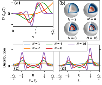
Figure 1: (a) Weight of the centroid spin magnitude $\bar{s}$ (arbitrary scaling). The negative regions grow in importance for increasing number of spins, $N$, but the number of nodes remains small. (b) Weight of $\bar{\bm{s}}$ with positive contributions in blue and negative in red. (c-d) Distribution of the $x$, $y$ (c) and $z$ (d) components of the spin centroid. The distributions become peaked around the quantum-mechanical values $\pm\tfrac{1}{2}$ with increasing $N$, and the relative peak heights approach the corresponding expectation values of the density matrix, here plotted for $\hat{\rho}=\frac{2}{3}|1\rangle\langle 1|+\frac{1}{3}|2\rangle\langle 2|$.

Results.—We have applied the spin path-integral method to Tully’s seminal scattering problems Tully (1990), which are well-known benchmark models but also proxies for realistic chemical reactions Ibele and Curchod (2020). The results are compared against calculations using numerically exact quantum mechanics as well as Ehrenfest dynamics and surface hopping. Simulation details are included in the Supplemental Material (SM) sup .

First, we consider the single avoided crossing (model I) with diabatic surfaces and coupling shown in the inset of Fig. 2. An initial Gaussian wavepacket enters from the left on the lower surface, $\psi_{1}(x,t=0)\otimes|1\rangle$, with enough kinetic energy that both product channels are open. Due to nonadiabatic coupling, the wavepacket splits into two separate wavepackets on the two surfaces and emerges as an entangled state, ${\psi_{1}(x,t=\infty)\otimes|1\rangle}+{\psi_{2}(x,t=\infty)\otimes|2\rangle}$, on the right. By quantum-classical entanglement, we mean that if the nuclei are in a certain region of phase space, then we know with certainty the quantum state of the electrons and vice versa. In Fig. 2 we show the distribution of the final momentum for two different initial energies. As is well known, Ehrenfest dynamics (MFT) is unable to capture the branching of the wavepacket, whereas surface hopping (FSSH) provides a reasonably accurate description for this model. The $N=1$ simulation predicts an envelope that covers the full range of momenta allowed by energy conservation, but lacks the two-peak structure. However, by increasing $N$, we find that the distribution smoothly splits into two parts and thus recovers the quantum-mechanical entanglement.

Figure 2: Probability distribution of the nuclear momentum after an avoided crossing (model I). The inset shows the diabatic potentials (solid lines) and coupling (dashed line). A wavepacket enters from the left on the lower surface with a narrow distribution of kinetic energies at roughly 1.5 (left panels) or 5 (right panels) times the asymptotic energy difference. Ehrenfest (MFT) gives a single peak around the average momentum, while linearized spin mapping ($N=1$) envelopes the exact wavepacket distribution. For higher $N$, the spin path-integral method correctly reproduces the wavepacket branching.

We emphasize that the dynamics consists of independent and deterministic trajectories on a weighted average of the two states, similar to both Ehrenfest dynamics and the linearized spin-mapping method, and the key difference lies in the weighting of the trajectories. Because the weights may be positive or negative, some of these cancel out in such a way that the ensemble branches when it emerges on uncoupled surfaces. This cancellation is reminiscent of more involved semiclassical methods such as Miller’s forward-backward propagator, which is also known to capture wavepacket splitting in the present model Sun and Miller (1997); Miller (2009, 2012). However, these approaches are inherently semiclassical, not classical, and include nuclear-coherence effects (to some level of approximation) via phases and prefactors that depend sensitively on the trajectory histories and make sampling difficult. The results of the simpler spin path-integral method demonstrate that only electronic coherence is necessary to recover the correct result. Although the trajectories also carry a sign, this depends in a relatively simple manner on a single degree of freedom, is fixed by the initial sampling, and is preserved by the dynamics.

For Tully’s dual avoided crossing (model II) we reach the same conclusions, and in the SM we show that the scattering probabilities are in good agreement with exact wavepacket calculations for a wide range of initial momenta sup .

Next, consider the more challenging extended coupling model (model III) shown in the inset of Fig. 3. As before, an initial wavepacket enters on the lower surface from the left but now the total energy is low enough for the upper channel to be closed on the right. During the collision, it thus splits into a transmitted part on the lower surface and a part on the upper surface which reflects and passes through the interaction region a second time. Surface hopping is well known to fail dramatically for systems with recrossing, because the electronic amplitudes picked up during the first crossing are inconsistent with the active surfaces Subotnik et al. (2016). This ‘overcoherence’ problem arises because the assumption of a unique trajectory for each electronic density matrix is not valid Subotnik et al. (2013) and is related to neglecting quantum-classical entanglement. Ehrenfest and various linearized mapping approaches have also been unable to describe this model Gao et al. (2020).

To quantify the overcoherence problems of quantum-classical simulations, we have calculated the time evolution of the impurity $S_{L}=1-\mathrm{tr}[\hat{\rho}^{2}]=2(\rho_{11}\rho_{22}-|\rho_{12}|^{2})$, which is a measure of entanglement and is related to the decoherence indicator studied in Ref. Min et al., 2015 with coupled-trajectory simulations. Here, $\rho_{nm}$ denotes elements of the reduced density matrix in the adiabatic representation and the results are shown in Fig. 3. Ehrenfest completely misses the second crossing at about 100 fs (since its trajectories do not reflect), and although some surface-hopping trajectories do reflect, FSSH is unable to correctly describe the entanglement in this system. The spin path-integral method on the other hand reproduces the correct result for this system.

Figure 3: Impurity in the extended coupling model (model III). The inset shows the adiabatic surfaces (solid) and nonadiabatic coupling (dashed). A wavepacket enters from the left and is partly reflected. Only the spin path-integral method with $N=4$ is able to correctly describe the second crossing of the interaction region (results for $N=8$, not shown, overlay with $N=4$).

Another well-known consequence of the overcoherence problems in surface hopping are erroneous oscillations Subotnik and Shenvi (2011b) in the scattering probabilities as shown in Fig. 4. For the spin path-integral method, we observe that the calculated scattering probabilities converge towards the correct values with increasing $N$ (although reproducing the step as the upper channel opens appears to be difficult). Note that we did not need to add ‘decoherence corrections’ for each trajectory (as is commonly done to fix surface hopping), but nevertheless do not observe the problems of overcoherence for the ensemble as a whole.

Figure 4: Transmission and reflection probabilities onto the adiabatic states in the extended coupling model (model III). While surface hopping (FSSH) suffers from erroneous oscillations, the spin path-integral method appears to be converging smoothly with increasing $N$ towards the exact scattering probabilities.

Finally, we note that unlike surface hopping, the results of the present method (like Ehrenfest and other mapping approaches Sun and Miller (1997); Cotton et al. (2017)) are not dependent on whether the adiabatic or diabatic representation is used.

Conclusions.—In this Letter we have showed that features of quantum-classical entanglement, such as wavepacket branching and impurity measurements, can indeed be captured by an ensemble of independent and deterministic classical trajectories. This discovery opens up for a new class of mixed quantum-classical methods, as an alternative to surface hopping, coupled-trajectory or semiclassical simulations. It also extends the applicability of mapping approaches, which have been successful for predicting electronic coherences but so far have struggled to describe the nuclear dynamics of scattering problems. The presented method relies on positive and negative trajectory weights whose sign cancellation does not become more difficult for larger systems or longer simulation time. We therefore expect it to be applicable to complex molecular systems and condensed-phase problems.

Here we have limited the treatment to two-level systems, but a multi-level extension already exists for linearized spin mapping Runeson and Richardson (2020) and the spin path-integral extension is straightforward (although there is no guarantee that $G_{N}$ will depend on only a scalar variable). Since the SW formalism can be applied to any symmetry group Tilma et al. (2016), a similar treatment could be made also in systems with different symmetries.

Particularly interesting is the case where $\hat{\rho}$ is a thermal density matrix. Since the weights are preserved by the dynamics, we expect this to be useful for equilibrium dynamics as the quantum Boltzmann distribution will automatically be conserved. The details are left to a forthcoming paper.