Chemical Abundance of the LINER galaxy UGC 4805 with SDSS-IV MaNGA

Abstract

Chemical abundance determinations in Low-Ionization Nuclear Line Regions (LINERs) are especially complex and uncertain because the nature of the ionizing source of this kind of object is unknown. In this work, we study the oxygen abundance in relation to the hydrogen abundance (O/H) of the gas phase of the UGC 4805 LINER nucleus. Optical spectroscopic data from the Mapping Nearby Galaxies (MaNGA) survey was employed to derive the O/H abundance of the UGC 4805 nucleus based on the extrapolation of the disk abundance gradient, on calibrations between O/H abundance and strong emission-lines for Active Galactic Nuclei (AGNs) as well as on photoionization models built with the Cloudy code, assuming gas accretion into a black hole (AGN) and post-Asymptotic Giant Branch (p-AGB) stars with different effective temperatures. We found that abundance gradient extrapolations, AGN calibrations, AGN and p-AGB photoionization models produce similar O/H values for the UGC 4805 nucleus and similar ionization parameter values. The study demonstrated that the methods used to estimate the O/H abundance using nuclear emission-line ratios produce reliable results, which are in agreement with the O/H values obtained from the independent method of galactic metallicity gradient extrapolation. Finally, the results from the WHAN diagram combined with the fact that the high excitation level of the gas has to be maintained at kpc scales, we suggest that the main ionizing source of the UGC 4805 nucleus probably has a stellar origin rather than an AGN.

1 Introduction

Determinations of the chemical abundances of Active Galactic Nuclei (AGNs) and Star-Forming regions (SFs) are essential for understanding the chemical evolution of galaxies and, consequently, of the Universe.

Among the heavy elements present in the gas phase of AGNs and SFs (e.g., O, N, S), oxygen is the element with more accurate abundance determinations. This is because prominent emission-lines from the main ionic stages of oxygen can be easily detected in the optical spectra of these objects, making it a good tracer of the metallicity (e.g., Kennicutt et al. 2003; Hägele et al. 2008; Dors et al. 2015, 2020a). Therefore, hereafter we use metallicity ($Z$) and oxygen abundance [12 + $\log$(O/H)] interchangeably. Abundance estimations based on the direct method, also known as $T_{\rm e}$-method, are commonly used to determine chemical abundances of gas phase of SFs (for a review see Peimbert et al. 2017; Pérez-Montero 2017). These estimations seem to be more reliable than those derived using empirical or theoretical relations between the different electron temperatures (Hägele et al., 2006, 2008). In fact, the compatibility between oxygen abundances in nebulae located in the solar neighborhood and the ones derived from observations of the weak interstellar O i$\lambda$1356 line towards the stars (see Pilyugin 2003 and references therein) sustains the accuracy of the $T_{\rm e}$-method. This method is based on determinations of nebular electron temperatures, which requires measurements of auroral emission-lines, such as [O iii]$\lambda$ 4363 and [N ii]$\lambda$ 5755, generally weak (about 100 times weaker than H$\beta$) or not measurable in objects with high metallicity and/or low excitation (e.g., van Zee et al. 1998; Díaz et al. 2007). In the cases that auroral lines can not be measured, indirect or strong-line methods can be used to estimate the oxygen abundance, as proposed by Jensen et al. (1976) and Pagel et al. (1979). This method is based on calibrations between the oxygen abundance or metallicity and strong emission-lines, easily measured in SF spectra (for a review see López-Sánchez & Esteban 2010b; Maiolino & Mannucci 2019; Kewley et al. 2019).

For AGNs, chemical abundance determinations are preferably carried out in Narrow Line Regions (NLRs) of Seyfert 2 nuclei due to the relatively low velocity ($v\>\la\>400\>\rm km\>s^{-1}$, Contini 2017) of the shock waves present in the gas and their low electron density ($N_{\rm e}\>\la\>2000\>\rm cm^{-3}$, Zhang et al. 2013; Dors et al. 2014; for a review see Dors et al. 2020a). Oxygen abundance estimations for NLRs of Seyfert 2 have been obtained by using the $T_{\rm e}$-method (Alloin et al. 1992; Izotov & Thuan 2008; Dors et al. 2015, 2020a) and strong-line methods (e.g., Storchi-Bergmann et al. 1998; Castro et al. 2017; Carvalho et al. 2020). Studies based on strong-line methods have indicated that Seyfert 2 nuclei in the local universe ($z\><\>0.4$) present similar metallicity (or abundances) as those in metal rich H ii regions, i.e., no extraordinary enrichment has been observed in AGNs, with these objects exhibiting solar or slightly over-solar metallicities. This result agrees with predictions of chemical evolution models for spiral and elliptical galaxies (e.g., Mollá & Díaz 2005).

An opposite situation is found for Low-Ionization Nuclear Emission-line Regions (LINERs), whose chemical abundance studies are rare in the literature. This class of objects appear in 1/3 of galaxies in the local universe (Netzer, 2013), and their ionization sources are still an open problem in astronomy. Heckman (1980) suggested that these nuclei have gas shocks as their main ionization/heating source. Later, Ferland & Netzer (1983) proposed that LINERs could be ionized by accretion gas into a central black hole (AGN) but with lower ionization parameters (U) than those found in Seyferts. Therefore, the difference between LINERs and other AGN types would consist of the order of the ionization parameter (Ho et al., 1993). However, Terlevich & Melnick (1985) and Shields (1992) proposed a new ionization model, i.e., LINERs are ionized by hot stars, but contrary to SFs, they are old stars (0.1-0.5 Gyr) that came out from the main sequence (e.g., in the post-Asymptotic Giant Branch, p-AGB). Based on this scenario, Taniguchi et al. (2000) showed that photoionization models considering Planetary Nebula Nuclei (PNNs) with a temperature of $10^{5}$ K as ionizing sources can reproduce the region occupied, at least, by a subset of type 2 LINERs in optical emission-line ratio diagnostic diagrams. Winkler (2014) found that these objects have composite ionizing sources, i.e., more than one mechanism is responsible for the ionization of the gas. This explanation was also proposed by Yan & Blanton (2012), Singh et al. (2013), and Bremer et al. (2013).

The unknown nature of the ionizing sources and excitation mechanisms of LINERs hinder determination of their metallicity using the $T_{\rm e}$-method and/or strong-line methods (e.g., Storchi-Bergmann et al. 1998). Annibali et al. (2010) analysed intermediate-resolution optical spectra of a sample of LINERs and derived oxygen abundances considering these objects as AGNs (by using the Storchi-Bergmann et al. 1998 calibrations) and as SFs (by using the Kobulnicky et al. 1999 calibration). These authors found that when AGNs are assumed as ionizing sources, higher oxygen values are derived than for those assuming hot stars, which provide sub-solar abundances. On the other hand, oxygen abundance estimations based on the extrapolation of disk abundance gradients to the central part of the galaxies (an independent method) by Florido et al. (2012) indicate over-solar oxygen abundances for three LINERs (NGC 2681, NGC 4314, and NGC 4394).

Recently, semi-empirical calibrations between the oxygen abundance (or metallicity) and strong-emission lines of Seyfert 2 were obtained by Castro et al. (2017) and Carvalho et al. (2020). In addition, several methods to determine the oxygen abundance gradients in spiral galaxies are available in the literature (see Vila-Costas & Edmunds, 1992; Zaritsky et al., 1994; van Zee et al., 1998; Pilyugin et al., 2004, 2007; Lopez-Sanchez & Esteban, 2010a). These methods, together with data from the Mapping Nearby Galaxies at the Apache Point Observatory (MaNGA, Bundy et al., 2015), offer a powerful opportunity to determine the chemical abundances of LINERs and to produce insights about the ionization mechanisms of these objects.

In previous papers, we have analysed oxygen abundance in Seyfert 2 nuclei using the $T_{\rm e}$-method, photoionization model grids, and HCM code (see Dors et al. 2014; Castro et al. 2017; Pérez-Montero et al. 2019; Dors et al. 2019; Carvalho et al. 2020; Dors et al. 2020a, b). Although, the semi-empirical calibrations between metallicity and strong-emission lines of Seyfert 2 obtained by Castro et al. 2017 and Carvalho et al. 2020 along with the AGN photoionization model grids and SF calibrations, are applied in this paper, the object class studied here and the methodology applied are also different. The main goal of this work is to determine the oxygen abundance in relation to the hydrogen abundance (O/H) in the central region of the LINER galaxy UGC 4805 (redshift $z=0.02698$), in combination with data from the Mapping Nearby Galaxies at the Apache Point Observatory (MaNGA, Bundy et al. (2015). We assumed a spatially flat cosmology with $H_{0}$ = 71 $\rm km\>s^{-1}Mpc^{-1}$, $\Omega_{m}=0.270$, and $\Omega_{\rm vac}=0.730$ (Wright, 2006), which leads to a spatial scale of 0.535 kpc/arcsec at the distance of UGC 4805. This paper is organized as follows: in Section 2 the observational data of UGC 4805 are described; Section 3 contains the methodology used to estimate the oxygen abundance of the nucleus and along the disk of UGC 4805; in Section 4, the results for the nuclear oxygen abundance are given; while discussion and conclusions of the outcome are presented in Sections 5 and  6, respectively.

2 Data

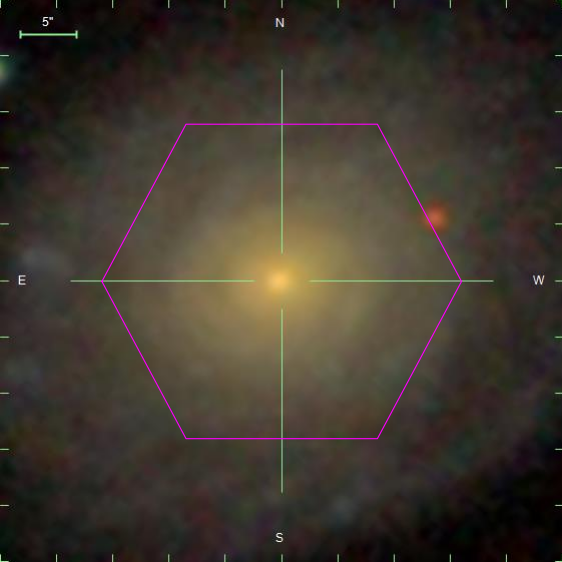
Figure 1: Left panel: SDSS false colour image combining the $gri$ bands of UGC 4805 taken from the MaNGA survey (Blanton et al., 2017). The IFU field of view is indicated in purple. Right panel: Map of the H$\alpha$ flux (in units of $10^{-17}$ erg/cm²/spaxel).

MaNGA survey is an Integral Field Spectroscopy (IFS) survey (Blanton et al., 2017) developed to observe about 10 000 galaxies until 2020 using Integral Field Units (IFUs). This survey is part of the fourth version of the Sloan Digital Sky Survey (SDSS-IV, Blanton et al. 2017) and utilises the 2.5 m Sloan Telescope in its spectroscopic mode. The spectra have a wavelength coverage of 3 600 - 10 300 Å, with a spectral resolution of $R\sim$ 1 400 at $\lambda\sim$4 000 Å  and $R\sim$ 2 600 at $\lambda\sim$9 000 Å. The angular size of each spaxel is 0.5 arcsec, and the average Full Width Half Maximum (FWHM) of the MaNGA data is 2.5 arcsec. For details about the strategy of observations and data reduction see Law et al. (2015) and Law et al. (2016), respectively. From the objects whose data are available in the MaNGA survey, we selected those presenting LINER nuclei and disk emission, preferably from objects classified as SFs. Based on these selection criteria, we selected 81 objects. In this work, we present a detailed analysis of the spiral galaxy UGC 4805, an object with a classical LINER nuclear emission and with the largest number of star-forming emission spaxels along the disk. The spectrum of each spaxel was processed according to the steps listed below:

• To obtain the nebular spectrum of each spaxel not contaminated by the stellar population continuum, i.e., the pure nebular spectrum, we use the stellar population synthesis code  STARLIGHT developed by Cid Fernandes et al. (2005); Mateus et al. (2006); Asari et al. (2007). This code fits the observed spectrum of a galaxy using a combination of Simple Stellar Populations (SSPs), in different proportions and excluding the emission lines. We use a spectral basis of 45 synthetic SSP spectra with three metallicities $Z$ = 0.004, 0.02 ($Z_{\odot}$), and 0.05, and 15 ages from 1 Myr up to 13 Gyr, taken from the evolutionary synthesis models of Bruzual & Charlot (2003). The reddening law by Cardelli et al. (1989) was considered. The stellar spectra of the SSPs were convolved with an elliptical Gaussian function to achieve the same spectral resolution as the observational data and transformed to the rest frame.
  

• The emission lines are fitted with Gaussian profiles. For more details about the synthesis method and the fitting of emission lines, see Zinchenko et al. (2016).
  

• The residual extinction associated with the gaseous component for each spatial bin was calculated by comparing the observed value of the H$\alpha$/H$\beta$ ratio to the theoretical value of 2.86 obtained by Hummer & Storey (1987) for an electron temperature of 10 000 K and an electron density of 100 cm^-3.

Fig. 1 presents the SDSS false colour image obtained combining the $gri$ bands of UGC 4805 and the resulting 2D map of the H$\alpha$ flux. Observe the very separated and clear nucleus and a bright star-forming ring in the disk at $\sim$8 arcsec ($\sim 4.2$ kpc). In Fig. 2 (top panel), the observed (in black) and synthetic (in red) spectra of the central region of UGC 4805 are shown. Fig. 2 (bottom panel) also presents the pure emission spectrum, i.e., after the SSP subtraction, as well as emission line identifications. The nuclear emission was obtained by integrating the flux of the central region considering a radius of 1.5 arcsec ($\sim$1 kpc), which corresponds approximately to the mean value of the seeing during the observations. In Table 1 the reddening corrected emission-line intensities (in relation to H$\beta$=100), the reddening function $f(\lambda)$, the logarithmic extinction coefficient $c$(H$\beta$), the visual extinction A_V, and the equivalent width of H$\alpha$ [$\rm W_{H\alpha}$] of the LINER nucleus of UGC 4805 are listed. The H$\beta$ luminosity (in units of erg/s) was also calculated and listed in Table 1, considering a distance of 119 Mpc.

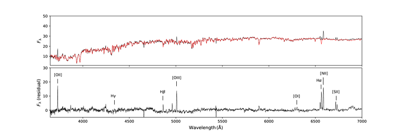
Figure 2: Upper panel: Stellar population synthesis for the nuclear region of UGC 4805 within a circular aperture with a radius equal to 1.5 arcsec ($\sim$1 Kpc). Observed and synthetic spectra are in black and red, respectively. Lower Panel: Pure emission spectrum of the UGC 4805 nucleus. Emission lines are identified in the plot. The flux is in units of $10^{-15}\rm{ergs}\,\rm{cm^{-2}}\,\rm{s^{-1}}\,\AA$.

The identification of the dominant ionization mechanism of the emitting gas across the galaxy is essential to determine chemical abundances. To do that, we used the $[\text{O\,{iii}}]\lambda 5007/\rm H\beta$ versus $[\text{N\,{ii}}]\lambda 6584/\rm H\alpha$, $[\text{O\,{iii}}]\lambda 5007/\rm H\beta$ versus $[\text{S\,{ii}}](\lambda\lambda 6716+31)/\rm H\alpha$, and $[\text{O\,{iii}}]\lambda 5007/\rm H\beta$ versus $[\text{O\,{i}}]\lambda 6300/\rm H\alpha$ diagnostic diagrams proposed by Baldwin et al. (1981), commonly known as BPT diagrams, to classify each spaxel of UGC 4805. The empirical and theoretical criteria proposed by Kewley et al. (2001) and Kauffmann et al. (2003), respectively, were considered to classify objects in H ii-like regions, composite, and AGN-like objects. Furthermore, the separation between Seyferts and LINERs proposed by Kewley et al. (2006) was used. Fig. 3 shows these BPT diagrams for each spaxel of UGC 4805 and the distribution of the regions in the galaxy according to $[\text{O\,{iii}}]/\rm H\beta$ versus $[\text{N\,{ii}}]/\rm H\alpha$ diagram. As can be seen in these diagrams, the central area of the galaxy is classified as LINER. Fig.  4 shows the same $[\text{O\,{iii}}]\lambda 5007/\rm H\beta$ versus $[\text{N\,{ii}}]\lambda 6584/\rm H\alpha$ diagram as Fig. 3 (top left panel), but as a function of the distance to the centre of the galaxy. The colour of each point corresponds to its distance from the galaxy centre, with the reddest points representing the central spaxels. As can be noted in this figure, the points closest to the centre lie in the LINER region. In Addition, the distance to the galaxy centre and the location in the diagram are connected, so that the points that approach the centre of the galaxy moves away from the line that separates SF-like objects from AGN-like ones.

On the other hand, the diagram introduced by Cid Fernandes et al. (2011) uses the equivalent width of H$\alpha$ ($\rm W_{H\alpha}$) and is known as a WHAN diagram. This diagram can to discriminate genuine low-ionization AGNs from galaxies that are ionized by evolved low-mass stars, i.e. the post-Asymptotic Giant Branch (post-AGB). The WHAN diagram identifies 5 classes of galaxies, namely:

1. Pure star forming galaxies: $\log(\text{N\,{ii}}/\rm H\alpha)\><\>-0.4$ and $\rm W_{H\alpha}\>>\>3$ Å.

2. Strong AGN (i.e., Seyferts): $\log(\text{N\,{ii}}/\rm H\alpha)\>>\>-0.4$ and $\rm W_{H\alpha}\>>\>6$ Å.

3. Weak AGN: $\log(\text{N\,{ii}}/\rm H\alpha)\>>\>-0.4$ and $\rm W_{H\alpha}$ between 3 and 6 Å.

4. Retired galaxies (i.e., fake AGN): $\rm W_{H\alpha}\><\>3$ Å.

5. Passive galaxies (actually, line-less galaxies): $\rm W_{H\alpha}$ and $\rm W_{\text{N\,{ii}}}\><\>0.5$ Å.

According to this classification, the UGC 4805 nucleus is a Retired Galaxy and, thus, it is ionized by post-AGB stars.

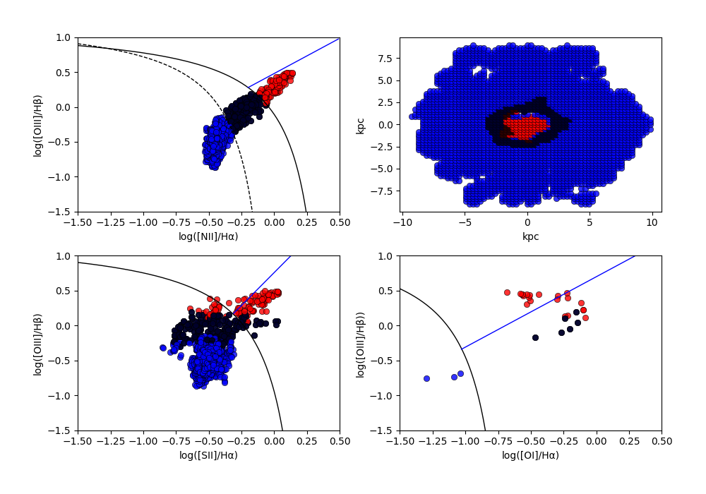
Figure 3: Top left panel: $\log([\text{O\,{iii}}]\lambda 5007/\rm H\beta)$ versus $\log([\text{N\,{ii}}]$ $\lambda 6584/\rm H\alpha)$ diagnostic diagram. Black solid curve represents the theoretical upper limit for the star-forming regions proposed by Kewley et al. 2001 (Ke01), the black dashed curve is the empirical star-forming limit proposed by Kauffmann et al. (2003) (Ka03), and the blue solid line represents the separation between Seyferts and LINERs from Kewley et al. (2006) (Ke06). The region between the Ke01 and Ka03 lines is denominated the composite region (black points). Top right panel: Distribution of the UGC 4805 regions accordingly to their main excitation mechanism as showed in the $\log([\text{O\,{iii}}]\lambda 5007/\rm H\beta)$ versus $\log([\text{N\,{ii}}]$ $\lambda 6584/\rm H\alpha)$ diagram (top left panel). Bottom left panel: $\log([\text{O\,{iii}}]\lambda 5007/\rm H\beta)$ versus $\log([\text{S\,{ii}}](\lambda\lambda 6716+31)/\rm H\alpha$) diagram. Bottom right panel: $\log([\text{O\,{iii}}]\lambda 5007/\rm H\beta)$ versus $\log([\text{O\,{i}}]\lambda 6300/\rm H\alpha)$ diagram. Red points represent the AGN-like spaxels and blue points the SF-like spaxels of UGC 4805, according to $\log([\text{O\,{iii}}]\lambda 5007/\rm H\beta)$ versus $\log([\text{N\,{ii}}]$ $\lambda 6584/\rm H\alpha)$ diagram.

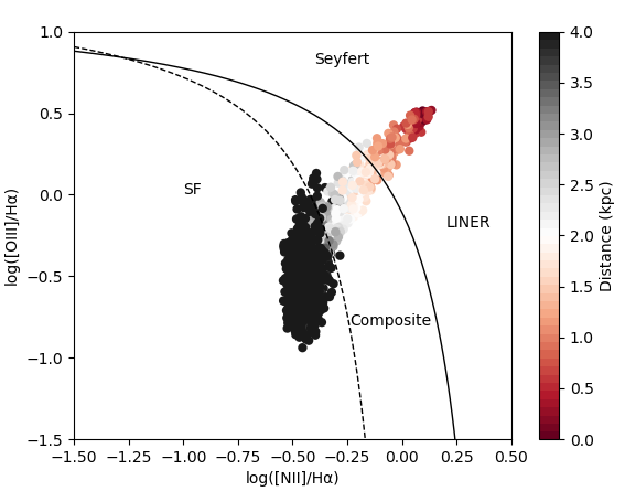
Figure 4: $\log([\text{O\,{iii}}]\lambda 5007/\rm H\beta)$ versus $\log([\text{N\,{ii}}]$ $\lambda 6584/\rm H\alpha)$ diagnostic diagram. The colour of each point corresponds to its distance from the galaxy centre, with the reddest points representing the central spaxels.

Table 1: Reddening corrected emission-line intensities (in relation to H$\beta$=100), reddening function $f(\lambda)$, the logarithmic extinction coefficient $c$(H$\beta$), the visual extinction A_V, and the H$\beta$ luminosity (erg/s) of the UGC 4805 nucleus. The estimations were obtained considering a radius of 1 kpc.

	$f(\lambda$)	Measurements
[O ii] $\lambda$3727	0.33	327 $\pm$ 5
[O iii] $\lambda$4959	$-$0.02	91 $\pm$ 2
H$\beta$ $\lambda$4861	0.00	100 $\pm$ 3
[O iii] $\lambda$5007	$-$0.04	242 $\pm$ 3
[N ii] $\lambda$6548	$-$0.35	126 $\pm$ 3
[O i] $\lambda$6300	$-$0.29	21 $\pm$ 5
H$\alpha$ $\lambda$6563	$-$0.35	286 $\pm$ 3
[N ii] $\lambda$6584	$-$0.35	321 $\pm$ 4
[S ii] $\lambda$6717	$-$0.36	135 $\pm$ 3
[S ii] $\lambda$6731	$-$0.37	96 $\pm$ 3
$c$(H$\beta$)	—	0.19 $\pm$ 0.005
WHα	—	1.65 $\pm$ 0.21 [Å]
AV	—	0.37 [mag]
$\log$[$L$(H$\beta$)]	—	38.86 [erg/s]

3 Oxygen abundance determination

To obtain the oxygen abundance of the UGC 4805 nucleus, five calibrations of SFs were used to extrapolate the radial oxygen abundance for the central region. This method has been used by several authors (e.g., Vila-Costas & Edmunds 1992; van Zee et al. 1998; Pilyugin et al. 2004; Zinchenko et al. 2019) and it produces an independent estimation of the oxygen abundance of nuclear regions. Recently, Mingozzi et al. (2020) measured gas-phase metallicity, ionisation parameter and dust extinction for a representative sample of 1795 local star-forming galaxies using integral field spectroscopy from the SDSS-IV MaNGA survey, showing the extensive reliability of this survey in this type of study. In addition, calibrations between the gas phase O/H abundance (or metallicity) and strong emission-lines for Seyfert 2 AGNs and photoionization model results were considered to estimate the UGC 4805 nucleus oxygen abundance. Each method is described below.

3.1 Star-forming regions

The goal of this work is to determine the oxygen abundance in the nuclear region of UGC 4805. In principle, determinations of oxygen abundances based on measurements of temperature sensitive line ratios, for example $[\text{O\,{iii}}]\lambda\,4363$ and $[\text{N\,{ii}}]\lambda\,5755$, should provide more accurate estimates of O/H (Kennicutt et al., 2003), because these are free from the uncertainties of photoionization models (e.g., Viegas 2002; Kennicutt et al. 2003), considered in the majority of strong-line methods (e.g., Kewley & Dopita 2002). Unfortunately, electron temperature sensitive line ratios were not measured in the UGC 4805 spectra. In these cases, only strong-line methods would be used to determine the oxygen abundances in the H ii regions along the UGC 4805 disk and, then, to obtain the central intersect O/H abundance. The strong-line methods considered in this work to derive the O/H gradient are briefly described below.

• Edmunds & Pagel (1984): This theoretical calibration, obtained by using the model calculations by Dufour et al. (1980) and Pagel et al. (1980), is based on the $R_{23}$=([O ii]$\lambda$3727+[O iii]$\lambda\lambda$4959+5007)/H$\beta$ index and the equations are given by

  $${}12+\log{\rm(O/H)_{up}}=8.76-0.69\log R_{23}$$ (1)

  and

  $${}12+\log{\rm(O/H)_{low}}=6.43+1.67\log R_{23},$$ (2)

  where "up" and "low" mean the equations for the upper and lower branch of the (O/H)-$R_{23}$ calibration, respectively.
  

• Denicoló et al. (2002): These authors proposed a calibration between the O/H abundance and the $N2=\log$([N ii]$\lambda$6584/H$\alpha$) line ratio, originally proposed by Storchi-Bergmann et al. (1994) as a metallicity indicator for H ii regions. For the low metallicity regime ($\rm 12+\log(O/H)\><\>8.4$), Denicoló et al. (2002) considered O/H values calculated through the $T_{\rm e}$-method and for the high metallicity regime abundance estimations based on calibrations by McGaugh (1991) and Díaz & Pérez-Montero (2000). The expression proposed by Denicoló et al. (2002) is

  $$12+\mathrm{\log(O/H)} =9.12+0.73\times N2.$$

  This calibration is valid for the range of $7.2<12+\mathrm{\log(O/H)}<9.1$.
  

• Pettini & Pagel (2004): These authors used a sample of extragalactic H ii regions and the $O3N2=\log\left(\frac{[\mathrm{OIII}]\lambda\,5007/\mathrm{H}\beta}{[\mathrm{NII}]\lambda\,6583/\mathrm{H}\alpha}\right)$ parameter to derive the calibration:

  $$12+\mathrm{\log(O/H)} =8.73-0.32\times\textit{O3N2},$$

  valid for the range of $8.0<12+\mathrm{\log(O/H)}<9.0$. Pettini & Pagel (2004) considered O/H values calculated using the $T_{\rm e}$-method for most cases and a few estimations based on detailed photoionization models.
  

• Dors & Copetti (2005): These authors built photoionization model sequences to reproduce the emission-line ratio intensities of H ii regions located along the disks of a sample of spiral galaxies to derive O/H gradients. Dors & Copetti (2005) obtained the semi-empirical calibration

  $$12+\mathrm{\log(O/H)} =8.96-0.03x-0.1x^{2}-0.21x^{3}-0.26x^{4},$$

  with $x=\log{R_{23}}$. This calibration is valid for the upper branch of the (O/H)-$R_{23}$ relation (i.e., $12+\log({\rm O/H})\>>\>8.2$).
  

• Pilyugin & Grebel (2016): These authors used a sample of H ii regions with abundances determined by the ‘counterpart’ method ($C$ method) to derive a calibration based on oxygen and nitrogen emission lines. These empirical calibrations use the excitation parameter $P=R_{3}/(R_{2}+R_{3})$, and $N2$, where $R_{2}$ = [O ii]($\lambda\,$3726 + $\lambda\,$3729)/H$\beta$ and $R_{3}$ = [O iii]($\lambda$ 4959 + $\lambda$ 500 7)/H$\beta$.

  Two equations were obtained, one for H ii regions with $N2\lid-0.6$ (the lower branch), defined by

  $$12+\log(\mathrm{O/H}) =7.932+0.944\times\log(R_{3}/R_{2})+0,695\times N2+$$

  $$\quad+(0.970-0.291\times\log(R_{3}/R_{2})+$$

  $$\quad-0.019\times N2)\times\log R_{2},$$

  and another for $N2\>\gid\>-0.6$ (the upper branch), where the following equation is valid

  $$12+\log(\mathrm{O/H}) =8.589+0.022\times\log(R_{3}/R_{2})+0.399\times N2+$$

  $$\quad+(-0.137+0.164\times\log(R_{3}/R_{2})+$$

  $$\quad+0.589\times N2)\times\log R_{2}.$$

This method is similar to the $C_{NS}$ method proposed by Pilyugin et al. (2012) and it yields O/H abundance values similar to those derived through the $T_{\rm e}$-method.

3.2 Active Galactic Nuclei

• Storchi-Bergmann et al. (1998): The first calibrations between the oxygen abundance and strong narrow emission-line ratios of AGNs were the theoretical ones proposed by Storchi-Bergmann et al. (1998). These authors used photoionization model sequences, built with the Cloudy code (Ferland, 1996), and proposed the calibrations

  $$\begin{matrix}(\mathrm{O/H})&=8.34+0.212x-0.012x^{2}-0.002y+0.007xy+\\ &\quad-0.002x^{2}y+6.52\times 10^{-4}y^{2}+2.27\times 10^{-4}xy^{2}+\\ &\quad+8.87\times 10^{-5}x^{2}y^{2},\end{matrix}$$

  $$\begin{matrix}(\mathrm{O/H})&=8.643-0.275u+0.164u^{2}+0.655v-0.154uv+\\ &\quad-0.021u^{2}v+0.288v^{2}+0.162uv^{2}+0.0353u^{2}v^{2},\end{matrix}$$

  where $x$ = [N ii]($\lambda\lambda$6548,6584)/H$\alpha$, $y=$ [O iii]($\lambda\lambda$4949,5007)/H$\beta$, $u=\log$([O ii]($\lambda\lambda$3726,3729)/[O iii]($\lambda\lambda$4959,5007), and $v=\log$ ([N ii]($\lambda\lambda$6548,6584)/H$\alpha)$.

  These calibrations are valid for the range of $8.4\><12+\>\mathrm{\log(O/H)}\>\><9.1$. Differences between O/H estimations derived using these calibrations are in of order of 0.1 dex (Storchi-Bergmann et al., 1998; Annibali et al., 2010; Dors et al., 2020a, 2015). For LINERs, Storchi-Bergmann et al. (1998) found that the calibrations above yield lower values than those derived from the extrapolation of O/H abundance gradients, suggesting that the assumptions of their models are not representative for LINERs. It should be mentioned that they indicated that their sample of LINERs was too small (only four objects) to provide a firm conclusion about the application of their method to this kind of object. They also suggest that a more extensive sample needs to be used to test their calibrations.
  

• Castro et al. (2017) proposed a semi-empirical calibration between the metallicity and the N2O2$=\log([\mathrm{\text{N\,{ii}}}]\lambda\,6584/[\mathrm{\text{O\,{ii}}}]\lambda\,3727)$ index. The calibration derived by these authors was obtained upon a comparison between observational and photoionization model predictions of the [O iii]$\lambda$5007/[O ii]$\lambda$3727 versus $N2O2$ line ratios and given by

  $$(Z/{\rm Z_{\odot}}) =1.08(\pm 0.19)\times N2O2^{2}+1.78(\pm 0.07)\times N2O2+$$

  $$\quad 1.24(\pm 0.01).$$

  This calibration is valid for $-1.4\>\la\>([\text{O\,{iii}}]/[\text{O\,{ii}}])\>\la\>2$ and $-1.0\>\la\>N2O2\>\la\>1$.
  

• Carvalho et al. (2020) used the same methodology as Castro et al. (2017) to calibrate NLRs metallicities of Seyfert 2 nuclei with the $N2$ emission-line ratio. This ratio is practically independent of the flux calibration and reddening correction. These authors proposed the following calibration

  $$(Z/Z_{\odot})=a^{N2}+b,$$ (3)

  where $a=4.01\pm 0.08$ and $b=-0.07\pm 0.01$. This calibration is valid for $-1.4\>\la\>([\text{O\,{iii}}]/[\text{O\,{ii}}])\>\la\>2$ and $-0.7\>\la\>(N2)\>\la\>0.6$. Carvalho et al. (2020) also proposed a relation between the ionization parameter ($U$) and the [O iii]$\lambda$5007/[O ii]$\lambda$3727 line ratio, almost independent of other nebular parameters, and given by

  $$\log U=(0.57\pm 0.01\>x^{2})+(1.38\pm 0.01\>x)-(3.14\pm 0.01),$$ (4)

  where $x=\log$([O iii]$\lambda$5007/[O ii]$\lambda$3727).

Although the AGN calibrations above were developed for Seyfert 2 nuclei, in this paper, we consider them to derive the O/H abundance in the LINER nucleus of UGC 4805, and we compared the resulting values to those derived from extrapolation of oxygen abundance gradients for central parts of this galaxy.

3.3 Photoionization models

To reproduce the observed line ratios of UGC 4805 LINER nucleus with the goal of deriving the O/H abundance and the ionization parameter ($U$), we built photoionization model grids using version 17.00 of the CLOUDY code (Ferland et al., 2017). These models are similar to the ones used in Carvalho et al. (2020), and a brief description of the input parameters is presented below:

1. SED: The models consider two distinct Spectral Energy Distributions (SEDs): one to represent an AGN and another representing p-AGB stars. The AGN SED is a multi-component continuum, similar to that observed in typical AGNs. As described in the Hazy manual of the Cloudy code , it is composed by the sum of two components. The first one is a Big Bump component peaking at $\approx$ 1 Ryd, parametrized by the temperature of the bump, assumed to be $5\>\times\>10^{5}$ K, with a high-energy exponential cutoff and an infrared exponential cutoff at 0.01 Ryd. The second component is an X-ray power law with spectral index $\alpha_{x}=-1$ that is only added for energies greater than 0.1 Ryd to prevent it from extending into the infrared. The X-ray power law is not extrapolated below 1.36 eV or above 100 keV: for energies lower than 1.36 eV it is set to zero (since the bump dominates for these energies), and for energies above 100 keV, the continuum falls off as $\nu^{-2}$. The $\alpha_{ox}$ spectral index defined as the slope of a power law between 2  keV and 2500 Å is the parameter that provides the normalization of the X-ray power law to make it compatible with the thermal component. It is given by

   $$\alpha_{ox}=\frac{\log[F(2\>{\rm keV})/F(2500\>\textrm{\AA})]}{\log[\nu(2\>{\rm keV})/\nu(2500\>\textrm{\AA})]},$$ (5)

   where $F$ is the flux at 2 keV, 2500 Å and $\nu$ are the corresponding frequencies (Tananbaum et al., 1979). This AGN SED generates a continuum similar to that used by Korista et al. (1997). In all our AGN models, a fixed value of $\alpha_{ox}=-1.0$ is assumed. Carvalho et al. (2020) found that models with $\alpha_{ox}\>\la\>-1.0$ trend not to reproduce optical emission line ratios of Seyfert 2 nuclei (see also Dors et al. 2017b; Pérez-Montero et al. 2019). Moreover, $\alpha_{ox}\sim-1.0$ has been derived in observational studies of LINERs and low luminosity AGNs (see Ho 1999; Eracleous et al. 2010; Maoz 2007; Younes et al. 2012).

   In the case of the stellar SED, we consider p-AGB stars atmosphere models by Rauch (2003) assuming the available values for the effective temperatures: $T_{\rm eff}=50,100$, and 190 kK, with the logarithm of the surface gravity $\log(\rm g)=6$. In Fig. 5, we present a comparison between the SEDs assumed in our models. The AGN SED maintains a high ionization flux even at high energies (low wavelengths) somewhat similar to the p-AGB one with the highest $T_{\rm eff}$ value. Some soft emission is noted for p-AGB stars with 100 kK and mainly with 50 kK. Both AGN and p-AGB SED models can be considered as the main ionizing source, i.e., responsible for the ionization of the gas, and underlying stellar population was not considered in the models. Therefore, our models are designed to investigate what kind of object would be producing the gas ionization in UGC 4805 based on emission line intensity ratios. These models are not intended for analysing the equivalent width of lines, as performed by Cid Fernandes et al. (2011), which also strongly depends on the underling stellar population (Dottori & Bica, 1981).

2. Metallicity: We assumed ($Z/{\rm Z_{\odot}}$) = 0.2, 0.5, 0.75, 1.0, 2.0, and 3.0 for the models. We assumed the solar oxygen abundance to be 12 + $\log$ (O/H)_⊙ = 8.69 (Asplund et al., 2009; Prieto et al., 2001) and it is equivalent to ($Z/{\rm Z_{\odot}}$)=1.0. All the abundances of heavy elements were scaled linearly with the metallicity, except the nitrogen for which we assumed the relation $\rm\log(N/O)=1.29\times[12+\log(O/H)]-11.84$ derived by Dors et al. (2017b), who considered abundance estimations for type 2 AGNs and H ii regions.
   

3. Electron Density: We assumed for the models an electron density value of $N_{\rm e}$ = 500 $\rm cm^{-3}$, constant in the nebular radius. This value is very similar to the one estimated for UGC 4805 nucleus through the relation between $N_{\rm e}$ and $R_{S2}=$[S ii]$\lambda 6716/\lambda 6731$ line ratio and using the IRAF/TEMDEN task. Observational estimations of $N_{\rm e}$ based on the Ar iv$\lambda$4711/$\lambda$4740 ratio, which map a denser gas region than the one based on [S ii] ratio, for two Seyfert nuclei (IC 5063 and NGC 7212) by Congiu et al. (2017), indicate $N_{\rm e}$ ranging from $\sim 200$ to $\sim 13\,000\>\,\rm cm^{-3}$. Furthermore, radial gradients with electron densities decreasing from the centres to the edges have been found in star-forming regions (e.g., Copetti et al. 2000) and in AGNs (e.g., Revalski et al. 2018). However, Carvalho et al. (2020) showed that models with $N_{\rm e}\><2\,000\>\rm cm^{-3}$ produce practically the same optical emission-line ratios. In addition, photoionization models assuming electron density variations along the radius have an almost negligible influence on predicted optical line ratios as demonstrated by Dors et al. (2019). For a detailed discussion about the $N_{\rm e}$ influence on metallicity estimates in Seyfert 2 AGNs, see Dors et al. (2020b).

4. Ionization Parameter: This parameter is defined as

   $$U=\frac{Q({\rm H)}}{4\,\pi\,R_{{\rm 0}}^{2}\,n(\rm H)\,\rm c},$$ (6)

   in which $Q(\rm H)$ [$\rm s^{-1}$] is the number of hydrogen-ionizing photons emitted by the central object, $R_{0}$ [cm] is the distance from the ionization source to the inner surface of the ionized gas cloud, $n(\rm H)$ [cm^-3] is the total hydrogen density (ionized, neutral and molecular), and $\rm c$ is the speed of light [cm s^-1]. We assumed logarithm of $U$ in the range of -4.0 $\leq\log U\leq$ -0.5, with a step of 0.5 dex, which is about the same range of values assumed by Feltre et al. (2016), who used a photoionization model grid to reproduce ultraviolet and optical emission-line ratios of active and normal galaxies. Different ionization parameter values simulate gas excitation differences, owing to variations in the mass of the gas phase and several geometrical conditions covering a wide range of possible scenarios (Pérez-Montero, 2014).

   In our models, a plane-parallel geometry is adopted, and the outer radius is assumed to be the one where the gas temperature falls to 4 000 K (default outer radius value in the CLOUDY code), since cooler gas practically does not produce optical emission lines. Models with different combinations of $Q(\rm H)$, $R_{0}$, and $n(\rm H)$, resulting in similar values of $U$, are homologous models, i.e., they predict very similar emission-line intensities.

   For the ionizing sources, Cloudy is a unidimensional code that assumes a central ionization source, which is a good approach for AGNs. However, in giant star-forming regions (e.g., Monreal-Ibero et al. 2011), stars are spreaded out through the gas. In this sense, in most cases, a central ionization source usage would not constitute a genuine representation of the situation. Ercolano et al. (2009) and Jamet & Morisset (2008) showed that the distribution of the O-B stars in relation to the gas alters the ionisation structure and the electron temperature. Hence, the ionization parameter partially depends on the distance of the ionizing source to the gas. However, in our case, we are considering an integrated spectrum of the UGC 4805 nucleus; thus, the stellar distribution may have a minimum effect on the emergent spectrum. In the case of giant H ii regions ionized by stellar clusters (e.g. Mayya & Prabhu 1996; Bosch et al. 2001), the hottest stars dominate the gas ionization (Dors et al., 2017a). Therefore, the assumption of a single star with a representative effective temperature as the main ionizing source, as assumed in our p-AGB models, is a good approximation (see e.g., Zinchenko et al., 2019).

To estimate the O/H and $U$ values for the UGC 4805 nucleus, we compare some observational emission line intensity ratios with photoionization model results using diagnostic diagrams and perform a linear interpolation between models.

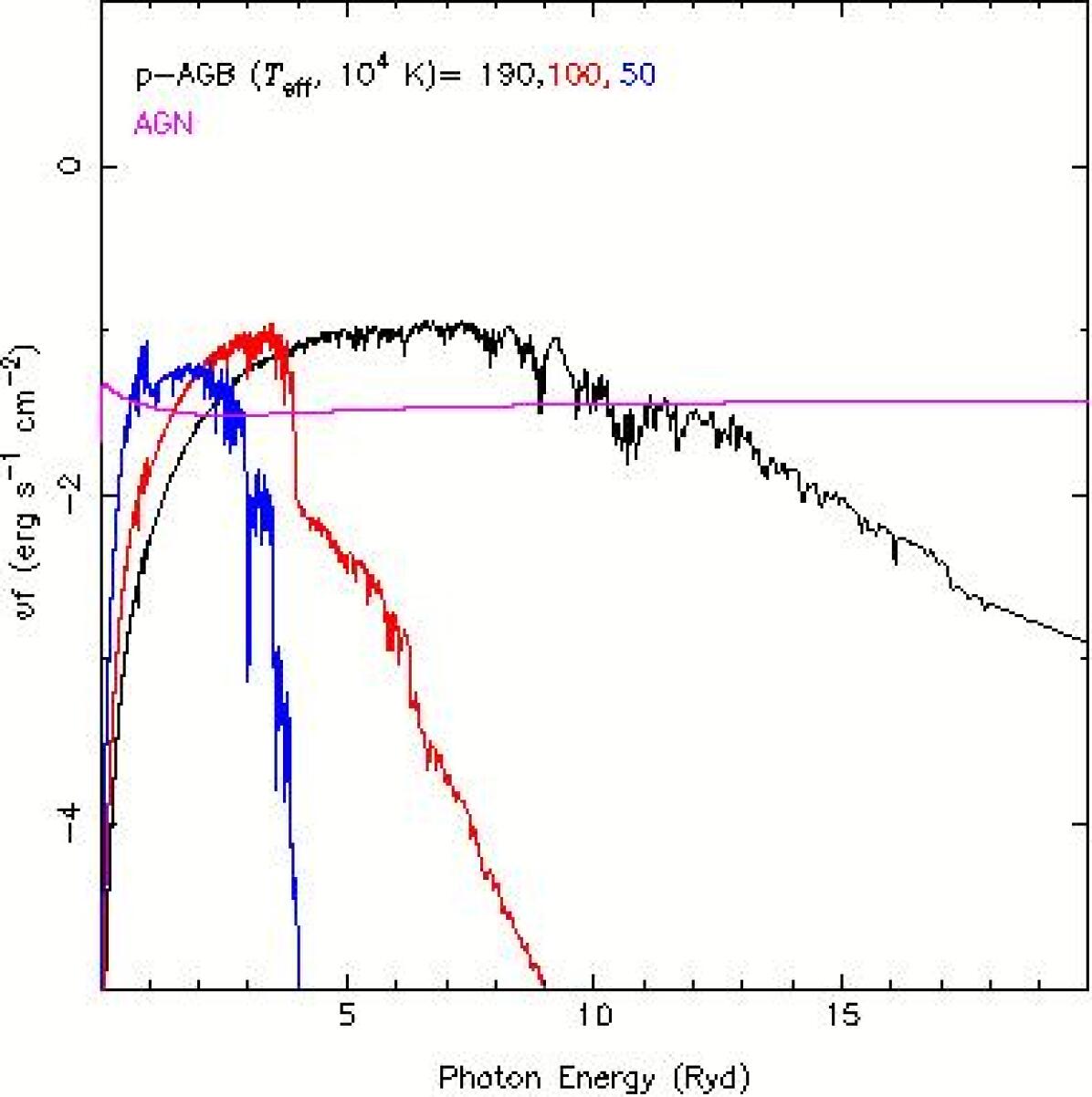
Figure 5: Comparison between the p-AGB star and AGN SEDs assumed the ionizing source in the photoionization models. The atmosphere models by Rauch (2003) and three effective temperature values (as indicated) are considered. The AGN SED is represented by a multi-component continuum with spectral index $\alpha_{ox}=-1.0$ (see Eq. 5).

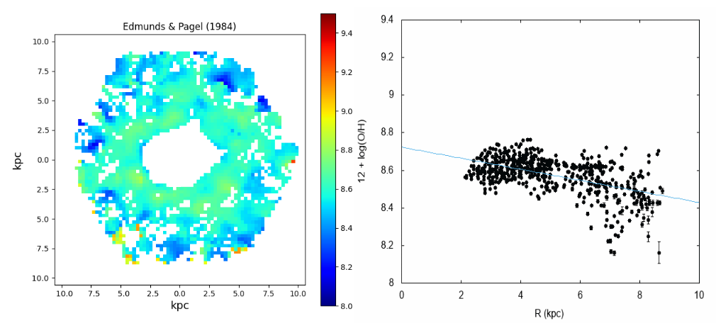
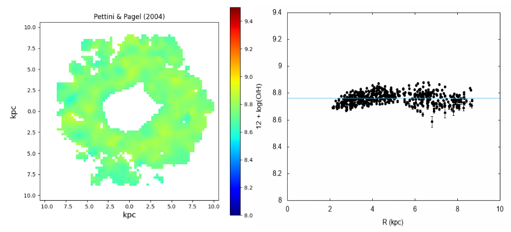
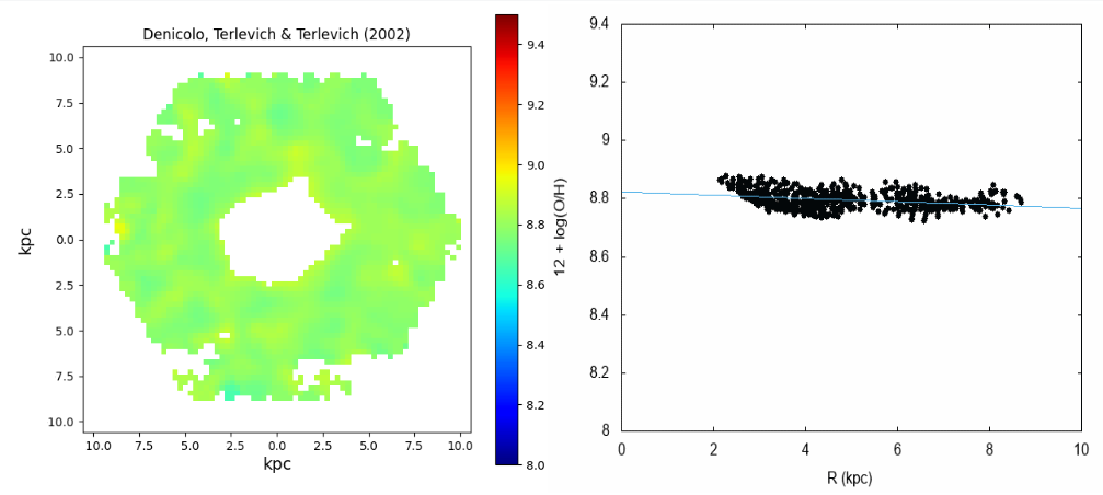
Figure 6: Left panels: oxygen abundance maps obtained through the calibrations described in Sect. 3.1 and indicated in each plot. Right panels: radial abundance distributions along the UGC 4805 disk. The line in each plot represents the linear fitting (Eq. 7) to the estimations, whose coefficients are listed in Table 2.

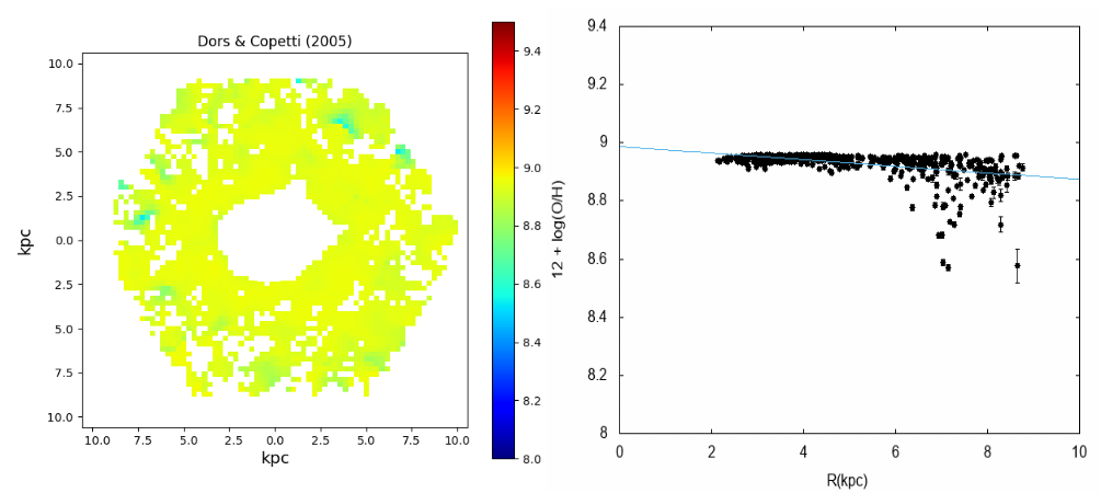
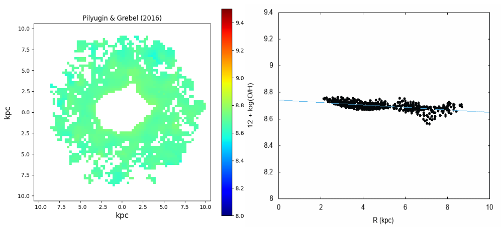
Figure 7: Same as Fig. 6, but for the indicated calibrations.

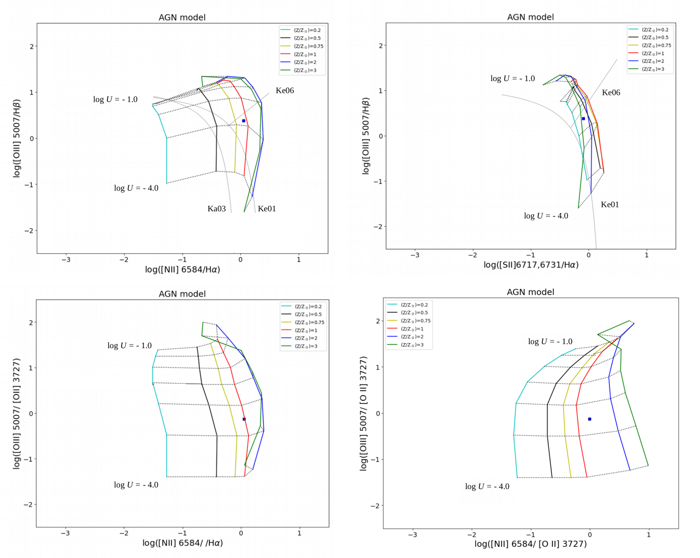
Figure 8: Upper left panel: $\log$([O iii]$\lambda 5007$/H$\beta$) versus $\log$([N ii]$\lambda 6584$/H$\alpha$) diagnostic diagram. Upper right panel: $\log$([O iii]$\lambda 5007$/H$\beta$) versus $\log$([S ii]$\lambda\lambda 6717,6731$/H$\alpha$) diagnostic diagram. Gray lines represent the separating criteria of the BPT diagrams, from Kewley et al. (2006) (Ke06), Kauffmann et al. (2003) (Ka03), and Kewley et al. (2001) (Ke01). Lower left panel: $\log$([O iii]$\lambda 5007$/[O ii] $\lambda 3727$) versus $\log$([N ii]$\lambda 6584$/H$\alpha$) diagnostic diagram. Lower right panel: $\log$([O iii]$\lambda 5007$/[O ii] $\lambda 3727$) versus $\log$([N ii]$\lambda 6584$/[O ii]$\lambda 3727$) diagnostic diagram. Coloured solid lines connect AGN photoionization model results (see Sect. 3.3) with the same metallicity $(Z/Z_{\odot})$ and dotted lines models with the same ionization parameter ($U$), as indicated. The blue point represents the observational line ratios for the UGC 4805 nucleus (see Sect. 2).

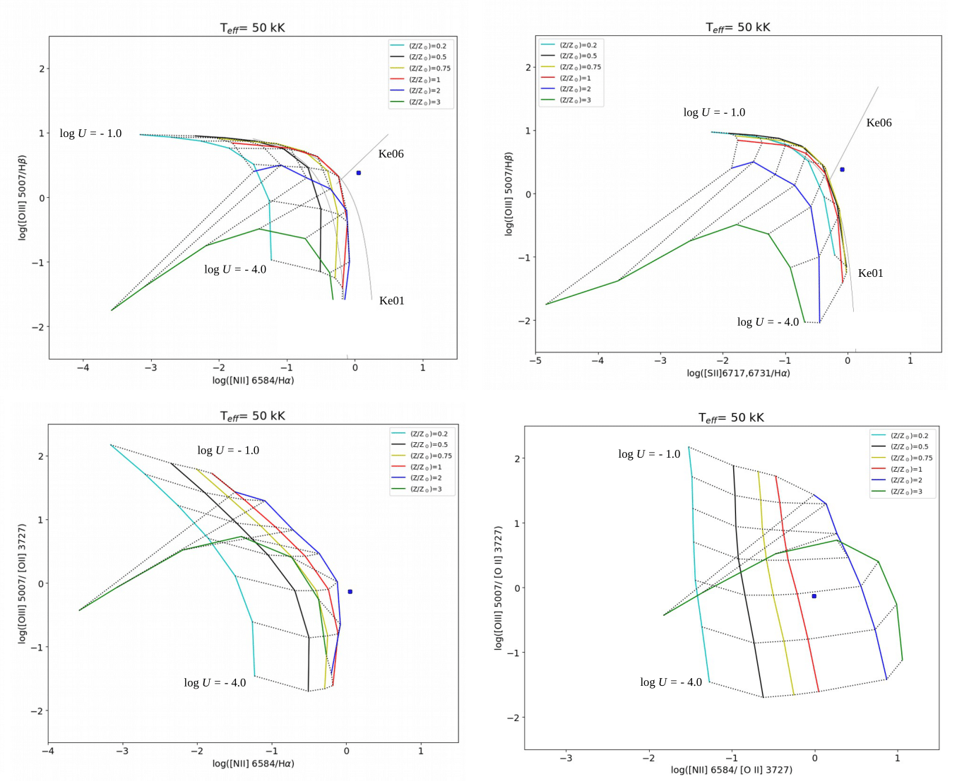
Figure 9: Same as Fig. 8 but considering p-AGB photoionization models (see Sect. 3.3) assuming $T_{\rm eff}$ = 50 kK.

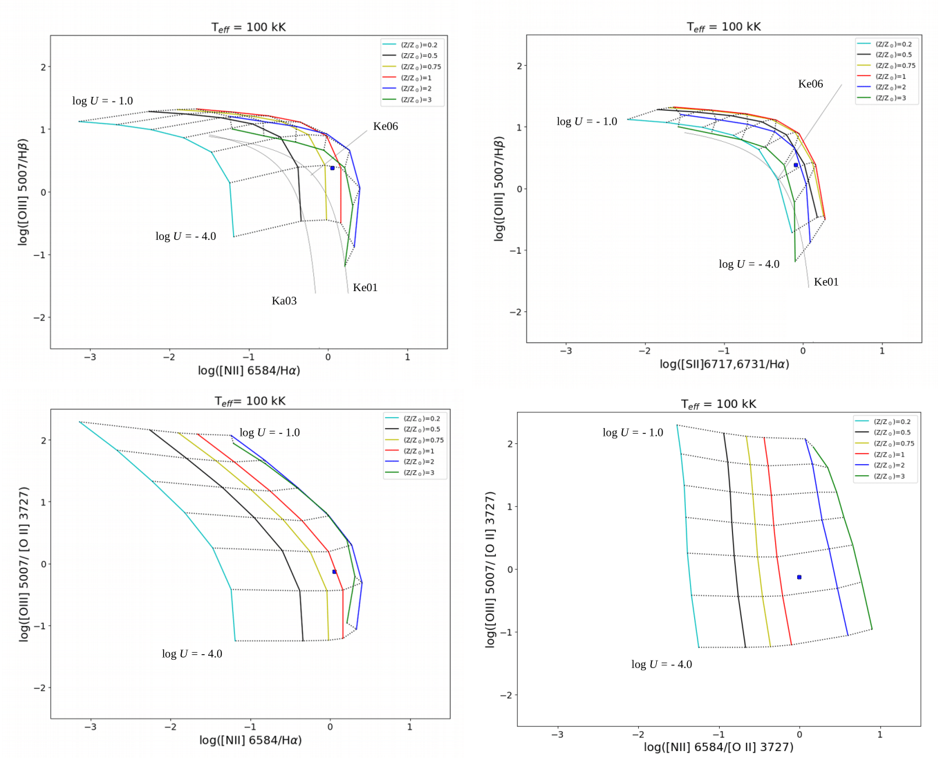
Figure 10: Same as Fig. 9 but considering p-AGB photoioniazation models (see Sect. 3.3) assuming $T_{\rm eff}$ = 100 kK.

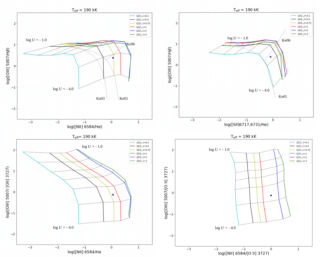
Figure 11: Same as Fig. 9 but considering p-AGB photoioniazation models (see Sect. 3.3) assuming $T_{\rm eff}$ = 190 kK.

4 Results

4.1 O/H calibrations

To apply some of the strong-line calibrations developed for SFs described in Sect. 3.1 to the UGC 4805 disk H ii regions, it is necessary to select which branch of the (O/H)-$R_{23}$ relation is adequate. We consider the Kewley & Ellison (2008) criteria to break the degeneracy, i.e., for objects with $\log$([N ii]$\lambda$6584/[O ii]$\lambda$3727)$\>>\>-1.2$, the upper $R_{23}$ branch must be used. The O/H abundances were estimated only for objects classified as pure star-forming regions, i.e., those with line ratios under the Kauffmann et al. (2003) line in the diagnostic diagram in the left panel of Fig. 3. Figures. 6 and  7 present the abundance maps (left panels) and the O/H values along the disk (right panels). Note that all the strong-line calibrations applied exhibited a linear decrease of O/H along the disk in agreement with previous results (e.g., Pilyugin et al. 2004). We derive the central oxygen abundance $\rm 12+\log(O/H)_{0}$ extrapolating to the centre of the galaxy the linear fit:

$${\rm 12+\log(O/H)=12+\log(O/H)_{0}}+(grad\>\times R),$$ (7)

where $\rm 12+\log(O/H)$ is the oxygen abundance at a given galactocentric distance $R$ (in units of arcsec) and $grad$ is the regression slope. The parameters of the linear regressions for the distinct calibrations used are listed in Table 2. The star-forming ring, clearly visible in the H$\alpha$ map (see Fig. 1), does not present any oxygen abundance discrepancy in comparison to its neighbour regions.

The calibration proposed by Edmunds & Pagel (1984) resulted in 12 + $\log$(O/H) values ranging from $\rm\sim 8.2$ to $\sim 8.8$ along the galactic disk, while the abundance value extrapolated to the nucleus ($R=0$ arcsec) is $\rm 12+\log(O/H)_{0}=8.72$. Considering the Denicoló et al. (2002) calibration, we derive 12 + $\log$ (O/H)₀ = 8.81 for the nucleus. By using the calibration by Pettini & Pagel (2004), we derive a nuclear abundance of 12 + $\log$ (O/H)₀ = 8.79. Estimates of oxygen abundances obtained using the calibration by Dors & Copetti (2005) yield a flatter gradient than the gradients derived with other calibrations, i.e., O/H values vary along the galactic disk in the narrow range of 8.85 < 12 + $\log$(O/H) < 9.0. The estimated nuclear abundance is 12 + $\log$ (O/H)₀ = 8.98. Note that a large part of our estimated values are close to the upper metallicity limit for this calibration, where the metallicity is practically constant, i.e., the O/H abundance is saturated with the variation of $R_{23}$. Finally, the application of the calibration proposed by Pilyugin & Grebel (2016) indicates abundances in the range of 8.5 < 12 + $\log$(O/H) < 8.7, with an inferred central abundance of 12 + $\log$ (O/H)₀ = 8.76, which is close to the abundance obtained through the Pettini & Pagel (2004) calibration. In summary, the extrapolation for the UGC 4805 LINER nucleus based on the calibrations considered above indicates an over solar oxygen abundance, with an averaged value of $\rm 12+\log(O/H)_{0}=8.82$.

To estimate the O/H abundance by using the nuclear emission of UGC 4805, we used the line intensity ratios listed in Table 1 and applied the Storchi-Bergmann et al. (1998), Castro et al. (2017), and Carvalho et al. (2020) calibrations. The estimated values of O/H abundance are listed in Table 2. As suggested by Storchi-Bergmann et al. (1998), the final (O/H) abundance derived from their methods should be the average of the values calculated from the two equations (Sect. 3.2), which provides 12 + $\log$ (O/H)₀ $=8.93\pm$ 0.04. The Castro et al. (2017) and Carvalho et al. (2020) calibrations provide a value of 12 + $\log$ (O/H)₀ = $8.77\pm$ 0.01 and 12 + $\log$ (O/H)₀ = $8.69\pm$ 0.01, respectively. An average value of 12 + $\log$ (O/H)${}_{0}=8.81\pm 0.02$ was derived considering the three calibrations.

Table 2: Oxygen abundance results for the UGC 4805 nucleus. The first set of values are the central Z/Z_⊙ estimations and the coefficients of the linear fitting (Eq. 7) to the O/H estimations along the UGC 4805 disk (see Figs. 6 and 7) considering different calibrations for H ii regions proposed by different authors as indicated (see Sect. 3.1). The second set of values are the metallicities, the oxygen abundances, and $\log U$ (only for one case) obtained by using the AGN calibrations (see Sect. 3.2). The third set of values are metallicities, O/H abundances and $\log U$ obtained from linear interpolations of the photoionization model results shown in Fig. 8, 9, 10 and 11. The diagnostic diagrams and the model ionizing sources considered are indicated.

Central intersect method – H ii region calibrations
	Z/Z⊙	12 + $\log$(O/H)0	grad (dex/arcsec)
Edmunds & Pagel (1984)	1.07	8.72 $\pm$ 0.003	$-0.016\pm 0.001$
Denicoló et al. (2002)	1.32	8.81 $\pm$ 0.002	$-0.002\pm 0.0001$
Pettini & Pagel (2004)	1.26	8.79 $\pm$ 0.003	$-0.003\pm 0.0002$
Dors & Copetti (2005)	1.95	8.98 $\pm$ 0.002	$-0.004\pm 0.0002$
Pilyugin & Grebel (2016)	1.17	8.76 $\pm$ 0.002	$-0.007\pm 0.0001$
Average	1.35	8.82 $\pm$ 0.003
AGN calibrations
	Z/Z⊙	12 + $\log$(O/H)	$\log U$
Storchi-Bergmann et al. (1998)	1.74	$8.93$ $\pm$ 0.04	—
Castro et al. (2017)	1.20	$8.77\pm 0.01$	—
Carvalho et al. (2020)	1.00	$8.69\pm 0.01$	$-3.09$
Average	1.31	8.81 $\pm$ 0.02
Diagnostic diagrams – Photoionization models
	Z/Z⊙	12 + $\log$(O/H)	$\log U$
AGN models
$\log([\text{O\,{iii}}]/\rm H\beta)$ vs. $\log$([N ii]/H$\alpha$)	0.95	$8.67\pm 0.02$	$-3.39$
$\log([\text{O\,{iii}}]/[\text{O\,{ii}}])$ vs. $\log$($[\text{N\,{ii}}]$/H$\alpha$)	0.93	$8.66\pm 0.02$	$-3.22$
$\log([\text{O\,{iii}}]/[\text{O\,{ii}}])$ vs. $\log([\text{N\,{ii}}]/[\text{O\,{ii}}])$	1.29	$8.80\pm 0.02$	$-3.24$
Average	1.06	$8.71\pm 0.02$
p-AGB models ($T_{\rm eff}$= 100 kK)
$\log([\text{O\,{iii}}]/\rm H\beta)$ vs. $\log$([N ii]/H$\alpha$)	0.85	$8.62\pm 0.03$	$-3.50$
$\log([\text{O\,{iii}}]/[\text{O\,{ii}}])$ vs. $\log$($[\text{N\,{ii}}]$/H$\alpha$)	0.98	$8.68\pm 0.01$	$-3.26$
$\log([\text{O\,{iii}}]/[\text{O\,{ii}}])$ vs. $\log([\text{N\,{ii}}]/[\text{O\,{ii}}])$	1.32	$8.81\pm 0.02$	$-3.29$
Average	1.06	$8.71\pm 0.02$
p-AGB models ($T_{\rm eff}$= 190 kK)
$\log([\text{O\,{iii}}]/\rm H\beta)$ vs. $\log$([N ii]/H$\alpha$)	0.72	$8.55\pm 0.01$	$-3.57$
$\log([\text{O\,{iii}}]/[\text{O\,{ii}}])$ vs. $\log$($[\text{N\,{ii}}]$/H$\alpha$)	0.81	$8.60\pm 0.01$	$-3.26$
$\log([\text{O\,{iii}}]/[\text{O\,{ii}}])$ vs. $\log([\text{N\,{ii}}]/[\text{O\,{ii}}])$	1.48	$8.86\pm 0.01$	$-3.31$
Average	1.00	$8.69\pm 0.01$

4.2 Photoionization models

As mentioned previously (see Sect. 3.3), two different photoionization model grids were built, one assuming an AGN as the ionizing source and another assuming p-AGB stars with different $T_{\rm{eff}}$ values as the ionizing source. In the upper panels of Fig. 8, the observational line ratios of the UGC 4805 nucleus are plotted in the $\log$([O iii]$\lambda 5007$/H$\beta$) versus $\log$([N ii]$\lambda 6584$/H$\alpha$) (left panel) and $\log$([O iii]$\lambda 5007$/H$\beta$) versus $\log$([S ii]$\lambda\lambda 6717,6731$/H$\alpha$) (right panel) diagnostic diagrams and compared to those predicted by AGN photoionization models. These plots also show the demarcation lines proposed by Kauffmann et al. (2003) and Kewley et al. (2006). The observational line intensity ratios are reproduced by the AGN models; therefore, we can infer a metallicity and an ionization parameter for the UGC 4805 nucleus. Using linear interpolation between the models in the $\log$([O iii]/H$\beta$) versus $\log$([N ii]/H$\alpha$) diagnostic diagram (Fig. 8 upper left panel), we derive a metallicity of (Z/Z_⊙) $\sim$ 0.95 and $\log U\sim-3.39$. For $\log$([O iii]/H$\beta$) versus $\log$([S ii]/H$\alpha$) diagnostic diagram (Fig. 8 upper right panel), which is clearly bi-valuated with the upper envelope at (Z/$\rm Z_{\odot})\sim$ 1, we adopt the models with larger values to characterise our object, since the low metallicity models do not represent AGN-like objects, as it is seen in the left panel. Then, we derived (Z/Z_⊙) $\sim$ 2.57 and $\log U\sim-3.26$, using the $\log$([O iii]/H$\beta$) versus $\log$([S ii]/H$\alpha$) diagnostic diagram. The second metallicity value is about three times the former one.

Dors et al. (2011), by using a grid of photoionization models, showed that there are relations between different line ratios, such as $[\text{O\,{iii}}]\lambda 5007$/$[\text{O\,{ii}}]\lambda 3727$ versus $[\text{N\,{ii}}]\lambda 6584$/H$\alpha$ and [O iii]$\lambda 5007$ / [O ii] $\lambda 3727$ versus [N ii]$\lambda 6584$/ [O ii]$\lambda 3727$, that are more sensitive to the ionization parameter, and the metallicities obtained through them are closer to those obtained using the $T_{\rm e}$-method. For this reason, we use these diagnostic diagrams also employed by Castro et al. (2017) and Carvalho et al. (2020) to perform a more reliable analysis. The lower panels of Fig. 8 presents these observational line ratios for the UGC 4805 nucleus superimposed on those ratios predicted by our AGN photoionization models. By using linear interpolation between the models we derive (Z/Z_⊙) $\sim$ 0.93 and $\log U\sim-3.22$ from the $\log$([O iii]/[O ii]) vs. $\log$([N ii]/H$\alpha$) diagnostic diagram (lower left panel), and (Z/Z_⊙) $\sim$ 1.29 and $\log U\sim-3.24$ from the $\log$([O iii]/[O ii]) vs. $\log$([N ii]/[O ii]) diagnostic diagram (lower right panel).

The values of the ionization parameter found using the four diagnostic diagrams (Fig. 8) are very similar and in agreement with the typical value for LINER galaxies estimated by Ferland & Netzer (1983).

Figs. 9, 10, and 11 contain the same diagnostic diagrams exhibited in Fig. 8 for the photoionization model results considering p-AGB stars as ionizing sources. In Fig. 9, the models with $T_{\rm eff}=50$ kK do not reproduce the UGC 4805 nucleus line ratios. In the upper panels of this figure, the parameter space characterized by the models is occupied only by H ii-like objects. Therefore, it is impossible to derive any value of $Z$ or $U$ from these models. For models with $T_{\rm eff}=100$ and 190 kK and considering the $\log$([O iii]/H$\beta$) versus $\log$([N ii]/H$\alpha$) (upper left panels of Figs. 10 and 11), we derive (Z/Z_⊙) $\sim$ 0.85 and $\log U\sim 3.50$, and (Z/Z_⊙) $\sim$ 0.72 and $\log U\sim 3.57$, respectively. Taking into account $T_{\rm eff}=100$ kK and $\log$([O iii]/H$\beta$) versus $\log$([S ii]/H$\alpha$) diagnostic diagram (upper right panel), we found $\log U\sim-3.44$ and two values for the metallicity, i.e., Z/$\rm Z_{\odot}\sim$ 2.87 and Z/$\rm Z_{\odot}\sim$ 0.42. This happens because, as in the case of AGN models, this relation is bi-valuated for the metallicity. Analysing the results of the same diagnostic diagram for the p-AGB models with $T_{\rm eff}=190$ kK, we do not observe a bi-valuated relatio. Models with metallicities larger than 0.75 occupy almost the same region. We obtain (Z/Z${}_{\odot})$ $\sim$ 0.36 and $\log U=-3.35$. These results could indicate that the high metallicity model solution found for the models with T${}_{\rm eff}=100$ kK [$(Z/\rm Z_{\odot})\sim 2.0$] is not correct.

The lower panels of Figs. 10 and 11 display the same diagnostic diagrams as in the lower panels of Fig. 8, but containing photoionization model results considering p-AGB stars as ionizing source. For models with $T_{\rm eff}=100$ kK (Fig. 10), we derive from the $\log$([O iii]/[O ii]) versus $\log$([N ii]/H$\alpha$) diagnostic diagram Z/$\rm Z_{\odot}\sim$ 0.98 and $\log U\sim-3.26$. From the $\log$([O iii]/[O ii]) versus $\log$([N ii]/[O ii]) diagram we calcule Z/$\rm Z_{\odot}\sim$ 1.32 and $\log U\sim-3.29$. Finally, we see that the models with $T_{\rm eff}=190$ kK (Fig. 11) provide from the $\log$([O iii]/[O ii]) versus $\log$([N ii]/H$\alpha$) diagram a metallicity of Z/$\rm Z_{\odot}\sim$ 0.81 and $\log U\sim-3.26$, and from the $\log$([O iii]/[O ii]) versus $\log$([N ii]/[O ii]) diagram Z/$\rm Z_{\odot}\sim$ 1.48 and $\log U\sim-3.31$.

The models yield bi-valuated or saturated results for the emission-line diagnostic diagrams that include the [S ii] emission-lines and show the more discrepant results including super-solar metallicities values [$(Z/Z_{\odot})\sim$ 2.57] for the AGN models and sub-solar metallicities for the p-AGB models with $T_{\rm eff}=100$ and 190 kK [$(Z/Z_{\odot})\sim$ 0.42, 0.36, respectively]. Hence, we do not take into account the results derived from the $\log$([O iii]/H$\beta$) versus $\log$([S ii]/H$\alpha$) diagnostic diagrams. The adopted $(Z/Z_{\odot})$, 12 + log(O/H) and $\log U$ values derived from Figs. 8, 10, and 11 are listed in Table 2.

The averaged values obtained from the extrapolation of the oxygen abundance gradient from H ii region estimations and from AGN calibrations are Z/Z${}_{\odot})\sim$ 1.35 and (Z/Z${}_{\odot})\sim$ 1.31, respectively. In both cases, the estimated abundance values are over-solar and are in agreement, taking into account their errors. On the other hand, all the photoionization model produce very similar average values close to the solar one: (Z/Z${}_{\odot})$ $\sim$ 1.06, 1.06, 1.00 for AGN, p-AGB with $T_{\rm eff}=100$ kK, and p-AGB with $T_{\rm eff}=190$ kK, respectively.

5 Discussion

A widely accepted practice is to estimate the oxygen abundance at the central part of a galaxy by the central intersect abundance [$\rm 12+\log(O/H)_{0}$] obtained from the radial abundance gradient (e.g., Vila-Costas & Edmunds 1992; Zaritsky et al. 1994; van Zee et al. 1998). This methodology has predicted solar or slightly over-solar metallicities for the central region of spiral galaxies, i.e., 12 + $\log$(O/H) from $\sim 8.6$ to $\sim 9.0$ (e.g., Pilyugin et al. 2004; Dors et al. 2020a), depending on the method considered to derive the individual disk H ii-region abundances. Comparisons of these extrapolated oxygen abundance measurements ($\rm 12+\log(O/H)_{0}$) with the ones obtained through the use of other methods that directly involve the nuclear emission have achieved good agreement. Storchi-Bergmann et al. (1998) found that the O/H abundances derived for a sample of seven Seyfert 2 galaxies through their calibrations are in consonance with those obtained by the central intersect abundance. This agreement was also found by Dors et al. (2015) using a larger sample of objects than the one considered by Storchi-Bergmann et al. (1998).

The oxygen abundance profile along the UGC 4805 disk presents a negative gradient, as expected, since it is a spiral galaxy. The negative gradient is explained naturally by models assuming the inside-out scenario of galaxy formation (Portinari & Chiosi, 1999; MacArthur et al., 2004; Barden et al., 2005). According to this scenario, galaxies begin to form in the inner regions before the outer regions. This was confirmed by studies of the stellar populations (e.g., Boissier & Prantzos 2000; Bell & Jong 2000; Pohlen & Trujillo 2006) and chemical abundances of spiral galaxies (e.g., Sánchez et al. 2014). As previously shown, considering the O/H gradient extrapolation, AGN calibrations, and AGN and p-AGB photoionization models, we derived averaged oxygen abundance values for the UGC 4805 nucleus in the range of 1.00 $\><\>$ (Z/Z${}_{\odot})\><$ 1.35, i.e., ranging from solar to slightly over-solar metallicities.

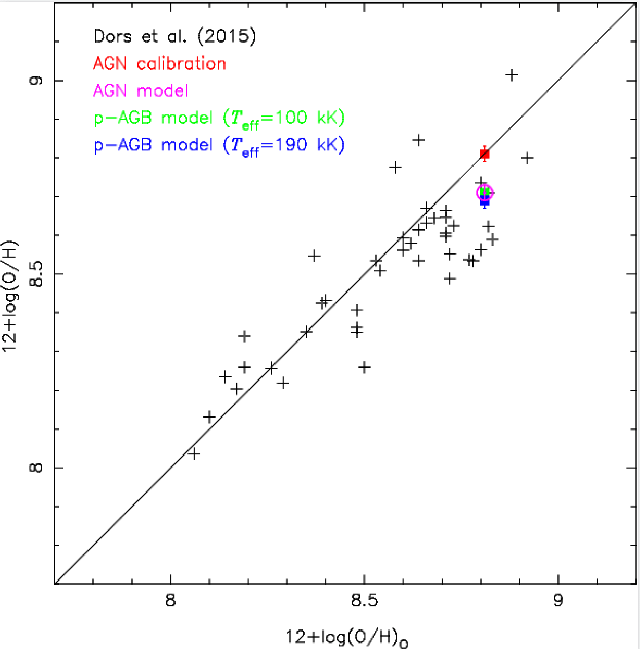
Figure 12: Comparison between central intersect oxygen abundances derived for the UGC 4805 nucleus from the radial abundance gradients ($12+\log(\rm O/H)_{0}$) with those derived through strong-line methods and AGN and p-AGB models (colored points as indicated). The point of the AGN model is the average from the AGN models. Black points represent the estimations performed by Dors et al. (2015) using the observational data by Ho et al. (1997). Solid line represents the equality between the estimations.

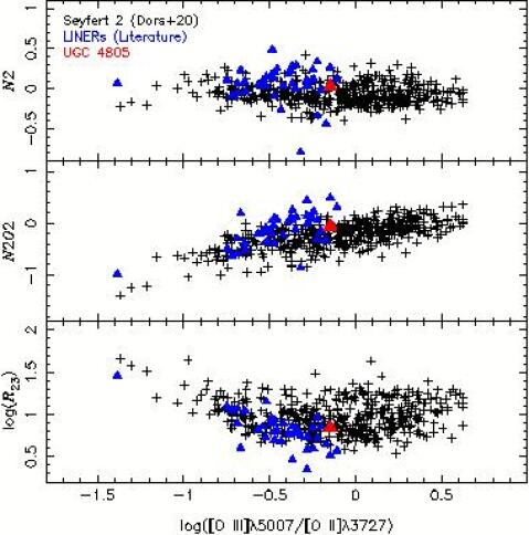
Figure 13: Metallicity sensitive line ratios $R_{23}$, $N2O2$ and $N2$ versus the ionization parameter sensitive line ratio [O iii]$\lambda$5007/[O ii]$\lambda$3727. Black points represent 463 Seyfert 2 nuclei studied by Dors et al. (2020a) and blue points represent 38 LINERs compiled by Ho et al. (1993), Eracleous & Halpern (2001), Annibali et al. (2010), and Molina et al. (2018). The red point represents the UGC 4805 nucleus.

In Fig. 12 the O/H average values estimated for the UGC 4805 nucleus using AGN calibrations as well as AGN and p-AGB models are compared with the average value derived through the central intersect method. The estimations for active and star-forming nuclei from Dors et al. (2015) are also presented in Fig. 12. This figure clearly illustrates that the averaged O/H value derived through the central intersect method is in consonance with the ones derived through the use of AGN calibrations and AGN and p-AGB models, as well as with the Dors et al. (2015) estimations.

Annibali et al. (2010) compared intermediate-resolution optical spectra of a sample of 49 nuclei classified as LINERs/composites with photoionization model results assuming as ionization source accretion-rate AGN (represented by a power law SED) using the Groves et al. (2004) models and the shock models built by Allen et al. (2008). These authors also compared the observed and predicted equivalent widths of the lines present on their spectra using models with p-AGB SEDs computed by Binette et al. (1994) [see also Cid Fernandes et al. 2009], finding that photoionization by p-AGB stars alone can explain only $\approx 22$% of the observed LINER/composite sample. They also found that the major fraction of their sample could be characterized by nuclear emission consistent with excitation by a low-accretion rate AGNs and/or fast shocks. Molina et al. (2018) compared observational optical and ultraviolet spectra of three LINERs with model results assuming four different excitation mechanisms: shocks, photoionization by an accreting black hole, and photoionization by young or old hot stars. These authors concluded that the model which best describes their data has a low-luminosity accretion-powered active nucleus that photoionizes the gas within $\sim 20$ pc of the galaxy centre, as well as shock excitation of the gas at larger distances. These authors also indicated that LINERs could have more than one ionizing mechanism. In the case of the UGC 4805 nucleus, the good agreement among all the different methods applied to derive its metallicity does not allow discrimination of the nature of the ionizing source.

Fig. 13 illustrates the $\log(R_{23})$, $N2O2$ and $N2$ metallicity indexes as a function of the [O iii]$\lambda$5007/[O ii]$\lambda$3727 line ratio used as an ionization parameter indicator for the UGC 4805 nucleus. This figure compares our results to those of a sample of confirmed 463 Seyfert 2 nuclei studied by Dors et al. (2020a) and obtained from the Sloan Digital Sky Survey (York et al., 2000), as well as those of a sample of 38 LINERs obtained by Ho et al. (1993), Eracleous & Halpern (2001), Annibali et al. (2010), and Molina et al. (2018). Both populations LINERs and Seyfert 2s, are partially overlapped in all of these diagrams although they display slightly different trends with LINERs showing lower ionizations ($\log U\><\>-3.2$) following Eq. 4. As can be seen in Fig. 13, the UGC 4805 nucleus positions in these diagrams are compatible with both populations, although they seems to follow the LINERs sequence; therefore, they would share similar physical properties.

According to Fig. 13, LINERs have intermediate and low [O iii]/[O ii] line ratio intensities, with the high values [$\rm(\log[\text{O\,{iii}}]/[\text{O\,{ii}}])\>\ga\>0.0$] only observed in Seyfert 2. Since the [O iii]/[O ii] has a strong dependence on $U$, the above results indicate a tendency of LINERs to present lower $U$ values than the ones in Seyfert 2, as suggested by Ferland & Netzer (1983). As an additional test of this scenario, Fig. 14 presents $\log U$ versus $Z/\rm Z_{\odot}$, calculated by using the Carvalho et al. (2020) calibrations (Eqs. 3 and 4), for the same sample as the one in Fig. 13. We can see that the UGC 4805 and the LINERs occupy the region with lower $U$ values and the highest values of this parameter are only observed in Seyfert 2s.

Finally, the geometry of UGC 4805 nucleus can provide information about the ionization source. In view of this, we compare the ionization parameter derived from the AGN and pAGB photoionization models with the one estimated from the observational data. The average value from the models is $<\log U>\sim-3.30$. To calculate $U$ from observational data, first, we obtained the $Q(\rm H)$ from the expression of Hekatelyne et al. (2018)

$$\left(\frac{Q({\rm H)}}{{\rm s^{-1}}}\right)=1.03\times 10^{12}\left(\frac{L_{\rm H_{\alpha}}}{\rm s^{-1}}\right)$$ (8)

and employing the luminosity value listed in Table 1. This luminosity value is obtained from integrated flux of the UGC 4805 nucleus. We found $\log Q({\rm H)}=50.87$. The value $N_{\rm e}=100\rm\>cm^{-3}$ is obtained from [S ii]$\lambda$6716/$\lambda 6731$ line ratio intensity, also listed in Table 1. Applying the $Q(\rm H)$ and $N_{\rm e}$ values above to Eq. 6, the innermost radius value $R_{0}$ to conciliate the theoretical and observational $U$ value is about 50 pc, in order of the radius assumed by Bennert et al. (2006). As can be noted in Fig. 3, the LINER emission extends to until $\sim 2.5$ kpc, i.e., a high excitation level (or $U$) is maintained from $\sim 50$ pc to kpc scales. Since $U\approx R^{-2}$, the ionization source is probably spread along the $R$. Thus, this result indicates that p-AGB is the preferable ionization source rather than AGN. This assumption is supported by the result obtained previously from the WHAN diagram (Cid Fernandes et al., 2011).

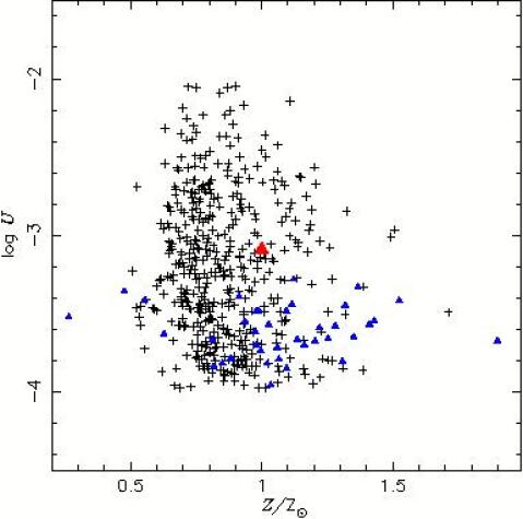
Figure 14: As Fig. 13 but for logarithm of the ionzation parameter ($\log U$) versus the metallicity ($Z/\rm Z_{\odot}$) calculated by using the Carvalho et al. (2020) calibrations (Eqs. 3 and 4).

6 Conclusion

We used optical emission-line fluxes taken from the SDSS-IV MaNGA survey to determine the oxygen abundance (metallicity) of the LINER nucleus of the UGC 4805 galaxy. The oxygen abundance was derived through the extrapolation of the radial abundance gradient for the central part of the disk by using strong-line calibrations for AGNs and photoionization model grids assuming as ionizing sources gas accretion into a black hole, representing an AGN and p-AGB stars. We found that all the O/H abundance estimations agree with each other. The results from these methods indicate that the UGC 4805 nucleus has an oxygen abundance in the range of $1.0\>\la\>(Z/Z_{\odot})\>\la 1.35$, i.e., solar or slightly over-solar metallicity.

We calculated that the UGC 4805 nucleus and other LINERs present metallicity and ionization parameter sensitive emission-line ratios similar to those observed in confirmed Seyfert 2 nuclei,l although exhibiting a slightly different trend. Even though LINERs present low ionization parameter values ($\log U\>\la\>-3.2$), Seyfert 2 nuclei also present low values of the ionization parameter. Although both AGN and p-AGB models (with $T_{\rm eff}$= 100 and 190 kK) are able to reproduce the observational data, the results from the WHAN diagram combined with the fact that the high excitation level of the gas has to be maintained at kpc scales, suggest that the main ionizing source of the UGC 4805 nucleus probably has a stellar origin rather than an AGN.

7 Data Availability

The data underlying this article will be shared on reasonable request to the corresponding author.

References

- Allen et al. (2008) Allen M. G., Groves B. A., Dopita M. A., Sutherland R. S., Kewley L. J., 2008, ApJS, 178, 20
- Alloin et al. (1992) Alloin D., Bica E., Bonatto C., Prugniel P., 1992, A&A, 266, 117
- Annibali et al. (2010) Annibali F., Bressan A., Rampazzo R., Zeilinger W. W., Vega O., Panuzzo P., 2010, A&A, 519, A40
- Asari et al. (2007) Asari N. V., Cid Fernandes R., Stasińska G., Torres-Papaqui J. P., Mateus A., Sodré L., Schoenell W., Gomes J. M., 2007, MNRAS, 381, 263
- Asplund et al. (2009) Asplund M., Grevesse N., Sauval A. J., Scott P., 2009, ARA&A, 47, 481
- Baldwin et al. (1981) Baldwin J. A., Phillips M. M., Terlevich R., 1981, PASP, 93, 5
- Barden et al. (2005) Barden M., et al., 2005, ApJ, 635, 959
- Bell & Jong (2000) Bell E. F., Jong R. S., 2000, MNRAS, 312, 497
- Bennert et al. (2006) Bennert N., Jungwiert B., Komossa S., Haas M., Chini R., 2006, A&A, 456, 953
- Binette et al. (1994) Binette L., Magris C. G., Stasińska G., Bruzual A. G., 1994, A&A, 292, 13
- Blanton et al. (2017) Blanton M. R., et al., 2017, AJ, 154, 28
- Boissier & Prantzos (2000) Boissier S., Prantzos N., 2000, in Franco J., Terlevich L., López-Cruz O., Aretxaga I., eds, Astronomical Society of the Pacific Conference Series Vol. 215, Cosmic Evolution and Galaxy Formation: Structure, Interactions, and Feedback. p. 53
- Bosch et al. (2001) Bosch G., Selman F., Melnick J., Terlevich R., 2001, A&A, 380, 137
- Bremer et al. (2013) Bremer M., Scharwächter J., Eckart A., Valencia-S. M., Zuther J., Combes F., Garcia-Burillo S., Fischer S., 2013, A&A, 558, A34
- Bruzual & Charlot (2003) Bruzual G., Charlot S., 2003, MNRAS, 344, 1000
- Bundy et al. (2015) Bundy K., et al., 2015, ApJ, 798, 7
- Cardelli et al. (1989) Cardelli J. A., Clayton G. C., Mathis J. S., 1989, ApJ, 345, 245
- Carvalho et al. (2020) Carvalho S. P., et al., 2020, MNRAS, 492, 5675
- Castro et al. (2017) Castro C. S., Dors O. L., Cardaci M. V., Hägele G. F., 2017, MNRAS, 467, 1507
- Cid Fernandes et al. (2005) Cid Fernandes R., Mateus A., Sodré L., Stasińska G., Gomes J. M., 2005, MNRAS, 358, 363
- Cid Fernandes et al. (2009) Cid Fernandes R., Schlickmann M., Stasinska G., Asari N. V., Gomes J. M., Schoenell W., Mateus A., Sodré L. J., 2009, The Starburst-AGN Disconnection: LINERs as Retired Galaxies. p. 122
- Cid Fernandes et al. (2011) Cid Fernandes R., Stasińska G., Mateus A., Vale Asari N., 2011, MNRAS, 413, 1687
- Congiu et al. (2017) Congiu E., et al., 2017, MNRAS, 471, 562
- Contini (2017) Contini M., 2017, MNRAS, 469, 3125
- Copetti et al. (2000) Copetti M. V. F., Mallmann J. A. H., Schmidt A. A., Castañeda H. O., 2000, A&A, 357, 621
- Denicoló et al. (2002) Denicoló G., Terlevich R., Terlevich E., 2002, MNRAS, 330, 69
- Díaz & Pérez-Montero (2000) Díaz A. I., Pérez-Montero E., 2000, MNRAS, 312, 130
- Díaz et al. (2007) Díaz Á. I., Terlevich E., Castellanos M., Hägele G. F., 2007, MNRAS, 382, 251
- Dors & Copetti (2005) Dors O. L., Copetti M. V. F., 2005, A&A, 437, 837
- Dors et al. (2011) Dors O. L. J., Krabbe A., Hägele G. F., Pérez-Montero E., 2011, MNRAS, 415, 3616
- Dors et al. (2014) Dors O. L., Cardaci M. V., Hägele G. F., Krabbe Â. C., 2014, MNRAS, 443, 1291
- Dors et al. (2015) Dors O. L., Cardaci M. V., Hägele G. F., Rodrigues I., Grebel E. K., Pilyugin L. S., Freitas-Lemes P., Krabbe A. C., 2015, MNRAS, 453, 4102
- Dors et al. (2017a) Dors O. L., Hägele G. F., Cardaci M. V., Krabbe A. C., 2017a, MNRAS, 466, 726
- Dors et al. (2017b) Dors O. L., Arellano-Córdova K. Z., Cardaci M. V., Hägele G. F., 2017b, MNRAS, 468, L113
- Dors et al. (2019) Dors O. L., Monteiro A. F., Cardaci M. V., Hägele G. F., Krabbe A. C., 2019, MNRAS, 486, 5853
- Dors et al. (2020a) Dors O. L., et al., 2020a, MNRAS, 492, 468
- Dors et al. (2020b) Dors O. L., Maiolino R., Cardaci M. V., Hägele G. F., Krabbe A. C., Pérez-Montero E., Armah M., 2020b, MNRAS, 496, 3209
- Dottori & Bica (1981) Dottori H. A., Bica E. L. D., 1981, A&A, 102, 245
- Dufour et al. (1980) Dufour R. J., Talbot R. J. J., Jensen E. B., Shields G. A., 1980, ApJ, 236, 119
- Edmunds & Pagel (1984) Edmunds M. G., Pagel B. E. J., 1984, MNRAS, 211, 507
- Eracleous & Halpern (2001) Eracleous M., Halpern J. P., 2001, ApJ, 554, 240
- Eracleous et al. (2010) Eracleous M., Hwang J. A., Flohic H. M. L. G., 2010, ApJS, 187, 135
- Ercolano et al. (2009) Ercolano B., Bastian N., Stasińska G., 2009, Ap&SS, 324, 199
- Feltre et al. (2016) Feltre A., Charlot S., Gutkin J., 2016, MNRAS, 456, 3354
- Ferland (1996) Ferland G. J., 1996, Hazy, A Brief Introduction to Cloudy 90
- Ferland & Netzer (1983) Ferland G. J., Netzer H., 1983, ApJ, 264, 105
- Ferland et al. (2017) Ferland G. J., et al., 2017, Rev. Mex. Astron. Astrofis., 53, 385
- Florido et al. (2012) Florido E., Pérez I., Zurita A., Sánchez-Blázquez P., 2012, A&A, 543, A150
- Groves et al. (2004) Groves B. A., Dopita M. A., Sutherland R. S., 2004, ApJS, 153, 75
- Hägele et al. (2006) Hägele G. F., Pérez-Montero E., Díaz Á. I., Terlevich E., Terlevich R., 2006, MNRAS, 372, 293
- Hägele et al. (2008) Hägele G. F., Díaz Á. I., Terlevich E., Terlevich R., Pérez-Montero E., Cardaci M. V., 2008, MNRAS, 383, 209
- Heckman (1980) Heckman T. M., 1980, A&A, 87, 152
- Hekatelyne et al. (2018) Hekatelyne C., et al., 2018, MNRAS, 479, 3966
- Ho (1999) Ho L. C., 1999, ApJ, 516, 672
- Ho et al. (1993) Ho L. C., Filippenko A. V., Sargent W. L. W., 1993, ApJ, 417, 63
- Ho et al. (1997) Ho L. C., Filippenko A. V., Sargent W. L. W., 1997, ApJS, 112, 315
- Hummer & Storey (1987) Hummer D. G., Storey P. J., 1987, MNRAS, 224, 801
- Izotov & Thuan (2008) Izotov Y. I., Thuan T. X., 2008, ApJ, 687, 133
- Jamet & Morisset (2008) Jamet L., Morisset C., 2008, A&A, 482, 209
- Jensen et al. (1976) Jensen E. B., Strom K. M., Strom S. E., 1976, ApJ, 209, 748
- Kauffmann et al. (2003) Kauffmann G., et al., 2003, MNRAS, 346, 1055
- Kennicutt et al. (2003) Kennicutt Robert C. J., Bresolin F., Garnett D. R., 2003, ApJ, 591, 801
- Kewley & Dopita (2002) Kewley L. J., Dopita M. A., 2002, ApJS, 142, 35
- Kewley & Ellison (2008) Kewley L., Ellison S., 2008, ApJ, 681, 1183
- Kewley et al. (2001) Kewley L. J., Dopita M. A., Sutherland R. S., Heisler C. A., Trevena J., 2001, ApJ, 556, 121
- Kewley et al. (2006) Kewley L. J., Groves B., Kauffmann G., Heckman T., 2006, MNRAS, 372, 961
- Kewley et al. (2019) Kewley L. J., Nicholls D. C., Sutherland R. S., 2019, ARA&A, 57, 511
- Kobulnicky et al. (1999) Kobulnicky H. A., Kennicutt Robert C. J., Pizagno J. L., 1999, ApJ, 514, 544
- Korista et al. (1997) Korista K., Baldwin J., Ferland G., Verner D., 1997, ApJS, 108, 401
- Law et al. (2015) Law D. R., et al., 2015, AJ, 150, 19
- Law et al. (2016) Law D. R., et al., 2016, AJ, 152, 83
- Lopez-Sanchez & Esteban (2010a) Lopez-Sanchez A. R., Esteban C., 2010a, arXiv e-prints,
- López-Sánchez & Esteban (2010b) López-Sánchez Á. R., Esteban C., 2010b, A&A, 517, A85
- MacArthur et al. (2004) MacArthur L. A., Courteau S., Bell E., Holtzman J. A., 2004, The Astrophysical Journal Supplement Series, 152, 175
- Maiolino & Mannucci (2019) Maiolino R., Mannucci F., 2019, A&ARv, 27, 3
- Maoz (2007) Maoz D., 2007, MNRAS, 377, 1696
- Mateus et al. (2006) Mateus A., Sodré L., Cid Fernand es R., Stasińska G., Schoenell W., Gomes J. M., 2006, MNRAS, 370, 721
- Mayya & Prabhu (1996) Mayya Y. D., Prabhu T. P., 1996, AJ, 111, 1252
- McGaugh (1991) McGaugh S. S., 1991, ApJ, 380, 140
- Mingozzi et al. (2020) Mingozzi M., et al., 2020, arXiv e-prints, p. arXiv:2002.05744
- Molina et al. (2018) Molina M., Eracleous M., Barth A. J., Maoz D., Runnoe J. C., Ho L. C., Shields J. C., Walsh J. L., 2018, ApJ, 864, 90
- Mollá & Díaz (2005) Mollá M., Díaz A. I., 2005, MNRAS, 358, 521
- Monreal-Ibero et al. (2011) Monreal-Ibero A., Relaño M., Kehrig C., Pérez-Montero E., Vílchez J. M., Kelz A., Roth M. M., Streicher O., 2011, MNRAS, 413, 2242
- Netzer (2013) Netzer H., 2013, The Physics and Evolution of Active Galactic Nuclei. Cambridge University Press, doi:10.1017/CBO9781139109291
- Pagel et al. (1979) Pagel B. E. J., Edmunds M. G., Blackwell D. E., Chun M. S., Smith G., 1979, MNRAS, 189, 95
- Pagel et al. (1980) Pagel B. E. J., Edmunds M. G., Smith G., 1980, MNRAS, 193, 219
- Peimbert et al. (2017) Peimbert M., Peimbert A., Delgado-Inglada G., 2017, PASP, 129, 082001
- Pérez-Montero (2014) Pérez-Montero E., 2014, MNRAS, 441, 2663
- Pérez-Montero (2017) Pérez-Montero E., 2017, PASP, 129, 043001
- Pérez-Montero et al. (2019) Pérez-Montero E., Dors O. L., Vílchez J. M., García-Benito R., Cardaci M. V., Hägele G. F., 2019, MNRAS, 489, 2652
- Pettini & Pagel (2004) Pettini M., Pagel B. E. J., 2004, MNRAS, 348, L59
- Pilyugin (2003) Pilyugin L. S., 2003, A&A, 399, 1003
- Pilyugin & Grebel (2016) Pilyugin L. S., Grebel E. K., 2016, MNRAS, 457, 3678
- Pilyugin et al. (2004) Pilyugin L. S., Vílchez J. M., Contini T., 2004, A&A, 425, 849
- Pilyugin et al. (2007) Pilyugin L. S., Thuan T. X., Vílchez J. M., 2007, MNRAS, 376, 353
- Pilyugin et al. (2012) Pilyugin L. S., Grebel E. K., Mattsson L., 2012, MNRAS, 424, 2316
- Pohlen & Trujillo (2006) Pohlen M., Trujillo I., 2006, A&A, 454, 759
- Portinari & Chiosi (1999) Portinari L., Chiosi C., 1999, A&A, 350, 827
- Prieto et al. (2001) Prieto C. A., Lambert D. L., Asplund M., 2001, ApJ, 556, L63
- Rauch (2003) Rauch T., 2003, A&A, 403, 709
- Revalski et al. (2018) Revalski M., et al., 2018, ApJ, 867, 88
- Sánchez et al. (2014) Sánchez S. F., et al., 2014, A&A, 563, A49
- Shields (1992) Shields J. C., 1992, ApJ, 399, L27
- Singh et al. (2013) Singh et al., 2013, A&A, 558, A43