Auxiliary iterative schemes for the discrete operators on de Rham complex

Abstract

The main difficulty in solving the discrete source or eigenvalue problems of the operator $d^{*}d$ with iterative methods is to deal with its huge kernel, for example, the $\nabla\times\nabla\times$ and $-\nabla\left(\nabla\cdot\right)$ operator. In this paper, we construct a kind of auxiliary schemes for their discrete systems based on Hodge Laplacian on de Rham complex. The spectra of the new schemes are Laplace-like. Then many efficient iterative methods and preconditioning techniques can be applied to them. After getting the solutions of the auxiliary schemes, the desired solutions of the original systems can be recovered or recognized through some simple operations. We sum these up as a new framework to compute the discrete source and eigenvalue problems of the operator $d^{*}d$ using iterative method. We also investigate two preconditioners for the auxiliary schemes, ILU-type method and Multigrid method. Finally, we present plenty of numerical experiments to verify the efficiency of the auxiliary schemes.

Keywords: de Rham complex, kernel, Maxwell equation, iterative method, multigrid method

1 Introduction

In this paper, we consider solving the algebraic systems involving the operator $d^{*}d$ Here, $d$ is the differential operator on the de Rham complex

$$\begin{split}\lx@xy@svg{\hbox{\raise 0.0pt\hbox{\kern 5.5pt\hbox{\ignorespaces\ignorespaces\ignorespaces\hbox{\vtop{\kern 0.0pt\offinterlineskip\halign{\entry@#!@&&\entry@@#!@\cr&&&&&\crcr}}}\ignorespaces{\hbox{\kern-5.5pt\raise 0.0pt\hbox{\hbox{\kern 0.0pt\raise 0.0pt\hbox{\hbox{\kern 3.0pt\raise 0.0pt\hbox{$\textstyle{0\ignorespaces\ignorespaces\ignorespaces\ignorespaces}$}}}}}}}\ignorespaces\ignorespaces\ignorespaces\ignorespaces{}{\hbox{\lx@xy@droprule}}\ignorespaces{\hbox{\kern 29.5pt\raise 0.0pt\hbox{\hbox{\kern 0.0pt\raise 0.0pt\hbox{\lx@xy@tip{1}\lx@xy@tip{-1}}}}}}{\hbox{\lx@xy@droprule}}{\hbox{\lx@xy@droprule}}{\hbox{\kern 29.5pt\raise 0.0pt\hbox{\hbox{\kern 0.0pt\raise 0.0pt\hbox{\hbox{\kern 3.0pt\raise 0.0pt\hbox{$\textstyle{V^{0}\ignorespaces\ignorespaces\ignorespaces\ignorespaces}$}}}}}}}\ignorespaces\ignorespaces\ignorespaces\ignorespaces{}{\hbox{\lx@xy@droprule}}\ignorespaces\ignorespaces\ignorespaces{\hbox{\kern 52.53386pt\raise 6.075pt\hbox{{}\hbox{\kern 0.0pt\raise 0.0pt\hbox{\hbox{\kern 3.0pt\hbox{\hbox{\kern 0.0pt\raise-3.075pt\hbox{$\scriptstyle{d^{0}}$}}}\kern 3.0pt}}}}}}\ignorespaces{\hbox{\kern 70.35556pt\raise 0.0pt\hbox{\hbox{\kern 0.0pt\raise 0.0pt\hbox{\lx@xy@tip{1}\lx@xy@tip{-1}}}}}}{\hbox{\lx@xy@droprule}}{\hbox{\lx@xy@droprule}}{\hbox{\kern 70.35556pt\raise 0.0pt\hbox{\hbox{\kern 0.0pt\raise 0.0pt\hbox{\hbox{\kern 3.0pt\raise 0.0pt\hbox{$\textstyle{V^{1}\ignorespaces\ignorespaces\ignorespaces\ignorespaces}$}}}}}}}\ignorespaces\ignorespaces\ignorespaces\ignorespaces{}{\hbox{\lx@xy@droprule}}\ignorespaces\ignorespaces\ignorespaces{\hbox{\kern 92.55052pt\raise 6.075pt\hbox{{}\hbox{\kern 0.0pt\raise 0.0pt\hbox{\hbox{\kern 3.0pt\hbox{\hbox{\kern 0.0pt\raise-3.075pt\hbox{$\scriptstyle{d^{1}}$}}}\kern 3.0pt}}}}}}\ignorespaces{\hbox{\kern 111.21112pt\raise 0.0pt\hbox{\hbox{\kern 0.0pt\raise 0.0pt\hbox{\lx@xy@tip{1}\lx@xy@tip{-1}}}}}}{\hbox{\lx@xy@droprule}}{\hbox{\lx@xy@droprule}}{\hbox{\kern 111.21112pt\raise 0.0pt\hbox{\hbox{\kern 0.0pt\raise 0.0pt\hbox{\hbox{\kern 3.0pt\raise 0.0pt\hbox{$\textstyle{\cdots\ignorespaces\ignorespaces\ignorespaces\ignorespaces}$}}}}}}}\ignorespaces\ignorespaces\ignorespaces\ignorespaces{}{\hbox{\lx@xy@droprule}}\ignorespaces\ignorespaces\ignorespaces{\hbox{\kern 130.00151pt\raise 6.075pt\hbox{{}\hbox{\kern 0.0pt\raise 0.0pt\hbox{\hbox{\kern 3.0pt\hbox{\hbox{\kern 0.0pt\raise-3.075pt\hbox{$\scriptstyle{d^{n-1}}$}}}\kern 3.0pt}}}}}}\ignorespaces{\hbox{\kern 148.71112pt\raise 0.0pt\hbox{\hbox{\kern 0.0pt\raise 0.0pt\hbox{\lx@xy@tip{1}\lx@xy@tip{-1}}}}}}{\hbox{\lx@xy@droprule}}{\hbox{\lx@xy@droprule}}{\hbox{\kern 148.71112pt\raise 0.0pt\hbox{\hbox{\kern 0.0pt\raise 0.0pt\hbox{\hbox{\kern 3.0pt\raise 0.0pt\hbox{$\textstyle{V^{n}\ignorespaces\ignorespaces\ignorespaces\ignorespaces}$}}}}}}}\ignorespaces\ignorespaces\ignorespaces\ignorespaces{}{\hbox{\lx@xy@droprule}}\ignorespaces{\hbox{\kern 190.12799pt\raise 0.0pt\hbox{\hbox{\kern 0.0pt\raise 0.0pt\hbox{\lx@xy@tip{1}\lx@xy@tip{-1}}}}}}{\hbox{\lx@xy@droprule}}{\hbox{\lx@xy@droprule}}{\hbox{\kern 190.12799pt\raise 0.0pt\hbox{\hbox{\kern 0.0pt\raise 0.0pt\hbox{\hbox{\kern 3.0pt\raise 0.0pt\hbox{$\textstyle{0}$}}}}}}}\ignorespaces}}}}\ignorespaces\end{split} \textstyle{0\ignorespaces\ignorespaces\ignorespaces\ignorespaces} \textstyle{V^{0}\ignorespaces\ignorespaces\ignorespaces\ignorespaces} \scriptstyle{d^{0}} \textstyle{V^{1}\ignorespaces\ignorespaces\ignorespaces\ignorespaces} \scriptstyle{d^{1}} \textstyle{\cdots\ignorespaces\ignorespaces\ignorespaces\ignorespaces} \scriptstyle{d^{n-1}} \textstyle{V^{n}\ignorespaces\ignorespaces\ignorespaces\ignorespaces} \textstyle{0} \textstyle{0\ignorespaces\ignorespaces\ignorespaces\ignorespaces} \textstyle{V^{0}\ignorespaces\ignorespaces\ignorespaces\ignorespaces} \scriptstyle{d^{0}} \textstyle{V^{1}\ignorespaces\ignorespaces\ignorespaces\ignorespaces} \scriptstyle{d^{1}} \textstyle{\cdots\ignorespaces\ignorespaces\ignorespaces\ignorespaces} \scriptstyle{d^{n-1}} \textstyle{V^{n}\ignorespaces\ignorespaces\ignorespaces\ignorespaces} \textstyle{0}$$ (1)

and $d^{*}$ is its adjoint operator. The main difficulty in solving such problems with iterative methods is to deal with the kernel of $d^{*}d$. We take $\mathbb{R}^{3}$ complex

$$\begin{split}\lx@xy@svg{\hbox{\raise 0.0pt\hbox{\kern 5.5pt\hbox{\ignorespaces\ignorespaces\ignorespaces\hbox{\vtop{\kern 0.0pt\offinterlineskip\halign{\entry@#!@&&\entry@@#!@\cr&&&&&\crcr}}}\ignorespaces{\hbox{\kern-5.5pt\raise 0.0pt\hbox{\hbox{\kern 0.0pt\raise 0.0pt\hbox{\hbox{\kern 3.0pt\raise 0.0pt\hbox{$\textstyle{0\ignorespaces\ignorespaces\ignorespaces\ignorespaces}$}}}}}}}\ignorespaces\ignorespaces\ignorespaces\ignorespaces{}{\hbox{\lx@xy@droprule}}\ignorespaces{\hbox{\kern 29.5pt\raise 0.0pt\hbox{\hbox{\kern 0.0pt\raise 0.0pt\hbox{\lx@xy@tip{1}\lx@xy@tip{-1}}}}}}{\hbox{\lx@xy@droprule}}{\hbox{\lx@xy@droprule}}{\hbox{\kern 29.5pt\raise 0.0pt\hbox{\hbox{\kern 0.0pt\raise 0.0pt\hbox{\hbox{\kern 3.0pt\raise 0.0pt\hbox{$\textstyle{H({\text{grad}})\ignorespaces\ignorespaces\ignorespaces\ignorespaces}$}}}}}}}\ignorespaces\ignorespaces\ignorespaces\ignorespaces{}{\hbox{\lx@xy@droprule}}\ignorespaces\ignorespaces\ignorespaces{\hbox{\kern 77.2639pt\raise 5.39166pt\hbox{{}\hbox{\kern 0.0pt\raise 0.0pt\hbox{\hbox{\kern 3.0pt\hbox{\hbox{\kern 0.0pt\raise-2.39166pt\hbox{$\scriptstyle{\nabla}$}}}\kern 3.0pt}}}}}}\ignorespaces{\hbox{\kern 95.87503pt\raise 0.0pt\hbox{\hbox{\kern 0.0pt\raise 0.0pt\hbox{\lx@xy@tip{1}\lx@xy@tip{-1}}}}}}{\hbox{\lx@xy@droprule}}{\hbox{\lx@xy@droprule}}{\hbox{\kern 95.87503pt\raise 0.0pt\hbox{\hbox{\kern 0.0pt\raise 0.0pt\hbox{\hbox{\kern 3.0pt\raise 0.0pt\hbox{$\textstyle{H({\text{curl}})\ignorespaces\ignorespaces\ignorespaces\ignorespaces}$}}}}}}}\ignorespaces\ignorespaces\ignorespaces\ignorespaces{}{\hbox{\lx@xy@droprule}}\ignorespaces\ignorespaces\ignorespaces{\hbox{\kern 138.06253pt\raise 5.68333pt\hbox{{}\hbox{\kern 0.0pt\raise 0.0pt\hbox{\hbox{\kern 3.0pt\hbox{\hbox{\kern 0.0pt\raise-2.1pt\hbox{$\scriptstyle{\nabla\times}$}}}\kern 3.0pt}}}}}}\ignorespaces{\hbox{\kern 159.47226pt\raise 0.0pt\hbox{\hbox{\kern 0.0pt\raise 0.0pt\hbox{\lx@xy@tip{1}\lx@xy@tip{-1}}}}}}{\hbox{\lx@xy@droprule}}{\hbox{\lx@xy@droprule}}{\hbox{\kern 159.47226pt\raise 0.0pt\hbox{\hbox{\kern 0.0pt\raise 0.0pt\hbox{\hbox{\kern 3.0pt\raise 0.0pt\hbox{$\textstyle{H({\text{div}})\ignorespaces\ignorespaces\ignorespaces\ignorespaces}$}}}}}}}\ignorespaces\ignorespaces\ignorespaces\ignorespaces{}{\hbox{\lx@xy@droprule}}\ignorespaces\ignorespaces\ignorespaces{\hbox{\kern 195.8702pt\raise 5.39166pt\hbox{{}\hbox{\kern 0.0pt\raise 0.0pt\hbox{\hbox{\kern 3.0pt\hbox{\hbox{\kern 0.0pt\raise-2.39166pt\hbox{$\scriptstyle{\nabla\cdot}$}}}\kern 3.0pt}}}}}}\ignorespaces{\hbox{\kern 219.98618pt\raise 0.0pt\hbox{\hbox{\kern 0.0pt\raise 0.0pt\hbox{\lx@xy@tip{1}\lx@xy@tip{-1}}}}}}{\hbox{\lx@xy@droprule}}{\hbox{\lx@xy@droprule}}{\hbox{\kern 219.98618pt\raise 0.0pt\hbox{\hbox{\kern 0.0pt\raise 0.0pt\hbox{\hbox{\kern 3.0pt\raise 0.0pt\hbox{$\textstyle{L^{2}\ignorespaces\ignorespaces\ignorespaces\ignorespaces}$}}}}}}}\ignorespaces\ignorespaces\ignorespaces\ignorespaces{}{\hbox{\lx@xy@droprule}}\ignorespaces{\hbox{\kern 259.59174pt\raise 0.0pt\hbox{\hbox{\kern 0.0pt\raise 0.0pt\hbox{\lx@xy@tip{1}\lx@xy@tip{-1}}}}}}{\hbox{\lx@xy@droprule}}{\hbox{\lx@xy@droprule}}{\hbox{\kern 259.59174pt\raise 0.0pt\hbox{\hbox{\kern 0.0pt\raise 0.0pt\hbox{\hbox{\kern 3.0pt\raise 0.0pt\hbox{$\textstyle{0}$}}}}}}}\ignorespaces}}}}\ignorespaces\end{split} \textstyle{0\ignorespaces\ignorespaces\ignorespaces\ignorespaces} \textstyle{H({\text{grad}})\ignorespaces\ignorespaces\ignorespaces\ignorespaces} \scriptstyle{\nabla} \textstyle{H({\text{curl}})\ignorespaces\ignorespaces\ignorespaces\ignorespaces} \scriptstyle{\nabla\times} \textstyle{H({\text{div}})\ignorespaces\ignorespaces\ignorespaces\ignorespaces} \scriptstyle{\nabla\cdot} \textstyle{L^{2}\ignorespaces\ignorespaces\ignorespaces\ignorespaces} \textstyle{0} \textstyle{0\ignorespaces\ignorespaces\ignorespaces\ignorespaces} \textstyle{H({\text{grad}})\ignorespaces\ignorespaces\ignorespaces\ignorespaces} \scriptstyle{\nabla} \textstyle{H({\text{curl}})\ignorespaces\ignorespaces\ignorespaces\ignorespaces} \scriptstyle{\nabla\times} \textstyle{H({\text{div}})\ignorespaces\ignorespaces\ignorespaces\ignorespaces} \scriptstyle{\nabla\cdot} \textstyle{L^{2}\ignorespaces\ignorespaces\ignorespaces\ignorespaces} \textstyle{0}$$ (2)

as an example to illustrate the problems that we want to deal with. The $0$-form $d^{*}d$ operator on this complex is the scalar Laplace operator $-\Delta$, the $1$-form is the Maxwell operator $\nabla\times\nabla\times$ and the $2$-form is the grad-div operator $-\nabla(\nabla\cdot)$.

When a new iterative method or preconditioning technique is proposed, the Laplace operator is always a standard test example. The high efficiency in solving the discrete Laplace problems is almost the basic requirement for a good iterative technique. There are plenty of iterative techniques satisfying such requirement [11, 21]. The main difference between the Laplace operator and the following two operators is the dimensions of their kernels. The kernel of the Laplace operator is usually caused by the shape of the domain or its boundary condition, and its dimension is a limited number. From the complex (54), we can find that the kernel of the Maxwell operator contains the space $\nabla H({\text{grad}})$ and the kernel of the grad-div operator contains the space $\nabla\times H({\text{curl}})$. They are both infinite dimensional. When discretizing the two operators, there exist huge kernels in their corresponding algebraic systems, especially for large-scale problems.

One of the two main feature of the multigrid method is error correction on the a coarse grid. We discretize the Maxwell equation

$$\begin{split}\nabla\times\nabla\times\mathbf{u}+c\mathbf{u}=\mathbf{f}\end{split}$$ (3)

using the first order edge finite element in a cubic domain $[0,1]^{3}$. We use a $100\times 100\times 100$ uniformly cubic mesh. Then the total degree of freedoms of the discrete problem of (3) is the number of the edges in this mesh, which is roughly $3\times 100^{3}=3,000,000$. The gradient of the nodal element space is contained in the kernel of the Maxwell operator $\nabla\times\nabla\times$, which means that the dimensional of the kernel of the discrete Maxwell operator is the number of the nodes in this mesh, about $100^{3}=1,000,000$. The frequencies of the modes in the $1,000,000$-dimensional kernel are all $c$ in the discrete system of (3). A nature coarse mesh is $50\times 50\times 50$. The degree of freedoms of this ’coarse’ problem is about $3\times 50^{3}=375,000$. This is even small than the dimension of the kernel (the low-frequency modes) of the ’fine’ problem. We could not expect that this ’coarse’ problem can correct the errors of the low-frequency modes with much larger dimension. The other feature of the multigrid method is smoothing on the ’fine’ grid. In fact, many smoothers that are efficient for the Laplace-like problems do not work for the discrete Maxwell problem.

The huge kernel also causes essential difficulty in solving the eigenvalue problem

$$\begin{split}\nabla\times\nabla\times\mathbf{u}=\lambda\mathbf{u}.\end{split}$$ (4)

The meaningful eigenpairs are two parts in practical applications. The first part are nonzero eigenvalues, especially some of the smallest nonzero eigenvalues. However, many iterative algorithms for matrix eigenvalue problems are efficient in finding the smallest or largest eigenvalues of a system [5]. The smallest eigenvalue of the discrete system of (4) is $0$ with the same dimension of the discrete kernel. This is the obstacle in front of the the smallest nonzero eigenvalues. The second part of the meaningful eigenpairs are the solenoidal and irrotational functions, whose corresponding eigenvalues are $0$. Then how to separate them from the large number of the eigenpairs with $0$ eigenvalue is a problem. Spectral inverse and shift or adding a Lagrange multiple can be a choice. The two methods involve solving linear systems. If the size of the discrete problem is not very large, the system can be solved by direct solver. When the size is large, the systems have to be solved by iterative method. Then it comes back to the problem of designing proper preconditioners again.

The efficient algorithms in solving the discrete systems involving the Maxwell operator and grad-div operator have been studied by many researchers. It is still an on-going topic. [12] proposed a multigrid method for Maxwell equation by treating the kernel and its orthogonal complement separately. [2] constructed proper Schwarz smoothers for multigrid in $H({\text{div}})$ and $H({\text{curl}})$. [15] proposed nodal auxiliary space preconditioners for the two spaces mainly based on regular decomposition. [14] constructed multilevel method for Maxwell and grad-div eigenvalue problems. To the author’s knowledge, the review of the researches on this problem is far from complete.

The approximation for $d^{*}d$ problems is also a very important problem. The discrete operator that we consider in this paper is base on these studies of approximation. We only cite some general results of them here. For details, we refer the readers to [3, 6, 7, 9, 8, 13, 16, 17] and the references therein.

In this paper, we construct a kind of auxiliary schemes for the $d^{*}d$ problems using Hodge Laplacian. The auxiliary part complements the kernel of the discrete $d^{*}d$ operator. Then the spectrum of the auxiliary schemes become Laplace-like. Both of the auxiliary source and eigenvalue problems can be computed in the same way as Laplace problem. Many efficient iterative methods and preconditioning techniques that are efficient for Laplace problem can be applied to the auxiliary schemes with some modifications. After obtaining the solutions of the auxiliary schemes, the desired solutions can be recovered or recognized through simple operations. We also consider the ILU-type method and multigrid method to solve the auxiliary schemes. Finial, we take the Maxwell and grad-div source and eigenvalue problems to verify the schemes.

The paper is organized as follows. In Section 2, we study the approximation of the abstract Hodge Laplacian on de Rham complex. In Section 3, we use the discrete Hodge Laplacian to construct auxiliary schemes for the discrete source and eigenvalue problems of $d^{*}d$ operator. In Section 4, we study the corresponding the matrix form of the auxiliary schemes and simplify them. In Section 5, we investigate two iterative methods, ILU-type preconditioning and multigrid method, to solve the auxiliary schemes. In Section 6, we take the source and eigenvalue of Maxwell and $-\nabla\left(\nabla\cdot\right)$ operator as examples to verify the efficiency of the auxiliary schemes. In Section 7, there are some conclusions.

2 The abstract Hodge Laplacian and its approximation

We study the Hodge Laplacian in the framework of the Hilbert complex. The de Rham complex is a typical example of the Hilbert complex when the operators are differential operators and the spaces are the corresponding function spaces. The main results in this section have been proved in [1, 3, 4]. We refer the readers to these references for more details.

2.1 The abstract Hodge Laplacian

Let us consider a Hilbert complex $(W,d)$. The $d^{k}$ is a closed densely defined operator from $W^{k}$ to $W^{k+1}$ and its domain is denoted by $V^{k}$. Then the corresponding domain complex is

$$\begin{split}\lx@xy@svg{\hbox{\raise 0.0pt\hbox{\kern 5.5pt\hbox{\ignorespaces\ignorespaces\ignorespaces\hbox{\vtop{\kern 0.0pt\offinterlineskip\halign{\entry@#!@&&\entry@@#!@\cr&&&&&\crcr}}}\ignorespaces{\hbox{\kern-5.5pt\raise 0.0pt\hbox{\hbox{\kern 0.0pt\raise 0.0pt\hbox{\hbox{\kern 3.0pt\raise 0.0pt\hbox{$\textstyle{0\ignorespaces\ignorespaces\ignorespaces\ignorespaces}$}}}}}}}\ignorespaces\ignorespaces\ignorespaces\ignorespaces{}{\hbox{\lx@xy@droprule}}\ignorespaces{\hbox{\kern 29.5pt\raise 0.0pt\hbox{\hbox{\kern 0.0pt\raise 0.0pt\hbox{\lx@xy@tip{1}\lx@xy@tip{-1}}}}}}{\hbox{\lx@xy@droprule}}{\hbox{\lx@xy@droprule}}{\hbox{\kern 29.5pt\raise 0.0pt\hbox{\hbox{\kern 0.0pt\raise 0.0pt\hbox{\hbox{\kern 3.0pt\raise 0.0pt\hbox{$\textstyle{V^{0}\ignorespaces\ignorespaces\ignorespaces\ignorespaces}$}}}}}}}\ignorespaces\ignorespaces\ignorespaces\ignorespaces{}{\hbox{\lx@xy@droprule}}\ignorespaces\ignorespaces\ignorespaces{\hbox{\kern 52.53386pt\raise 6.075pt\hbox{{}\hbox{\kern 0.0pt\raise 0.0pt\hbox{\hbox{\kern 3.0pt\hbox{\hbox{\kern 0.0pt\raise-3.075pt\hbox{$\scriptstyle{d^{0}}$}}}\kern 3.0pt}}}}}}\ignorespaces{\hbox{\kern 70.35556pt\raise 0.0pt\hbox{\hbox{\kern 0.0pt\raise 0.0pt\hbox{\lx@xy@tip{1}\lx@xy@tip{-1}}}}}}{\hbox{\lx@xy@droprule}}{\hbox{\lx@xy@droprule}}{\hbox{\kern 70.35556pt\raise 0.0pt\hbox{\hbox{\kern 0.0pt\raise 0.0pt\hbox{\hbox{\kern 3.0pt\raise 0.0pt\hbox{$\textstyle{V^{1}\ignorespaces\ignorespaces\ignorespaces\ignorespaces}$}}}}}}}\ignorespaces\ignorespaces\ignorespaces\ignorespaces{}{\hbox{\lx@xy@droprule}}\ignorespaces\ignorespaces\ignorespaces{\hbox{\kern 92.55052pt\raise 6.075pt\hbox{{}\hbox{\kern 0.0pt\raise 0.0pt\hbox{\hbox{\kern 3.0pt\hbox{\hbox{\kern 0.0pt\raise-3.075pt\hbox{$\scriptstyle{d^{1}}$}}}\kern 3.0pt}}}}}}\ignorespaces{\hbox{\kern 111.21112pt\raise 0.0pt\hbox{\hbox{\kern 0.0pt\raise 0.0pt\hbox{\lx@xy@tip{1}\lx@xy@tip{-1}}}}}}{\hbox{\lx@xy@droprule}}{\hbox{\lx@xy@droprule}}{\hbox{\kern 111.21112pt\raise 0.0pt\hbox{\hbox{\kern 0.0pt\raise 0.0pt\hbox{\hbox{\kern 3.0pt\raise 0.0pt\hbox{$\textstyle{\cdots\ignorespaces\ignorespaces\ignorespaces\ignorespaces}$}}}}}}}\ignorespaces\ignorespaces\ignorespaces\ignorespaces{}{\hbox{\lx@xy@droprule}}\ignorespaces\ignorespaces\ignorespaces{\hbox{\kern 130.00151pt\raise 6.075pt\hbox{{}\hbox{\kern 0.0pt\raise 0.0pt\hbox{\hbox{\kern 3.0pt\hbox{\hbox{\kern 0.0pt\raise-3.075pt\hbox{$\scriptstyle{d^{n-1}}$}}}\kern 3.0pt}}}}}}\ignorespaces{\hbox{\kern 148.71112pt\raise 0.0pt\hbox{\hbox{\kern 0.0pt\raise 0.0pt\hbox{\lx@xy@tip{1}\lx@xy@tip{-1}}}}}}{\hbox{\lx@xy@droprule}}{\hbox{\lx@xy@droprule}}{\hbox{\kern 148.71112pt\raise 0.0pt\hbox{\hbox{\kern 0.0pt\raise 0.0pt\hbox{\hbox{\kern 3.0pt\raise 0.0pt\hbox{$\textstyle{V^{n}\ignorespaces\ignorespaces\ignorespaces\ignorespaces}$}}}}}}}\ignorespaces\ignorespaces\ignorespaces\ignorespaces{}{\hbox{\lx@xy@droprule}}\ignorespaces{\hbox{\kern 190.12799pt\raise 0.0pt\hbox{\hbox{\kern 0.0pt\raise 0.0pt\hbox{\lx@xy@tip{1}\lx@xy@tip{-1}}}}}}{\hbox{\lx@xy@droprule}}{\hbox{\lx@xy@droprule}}{\hbox{\kern 190.12799pt\raise 0.0pt\hbox{\hbox{\kern 0.0pt\raise 0.0pt\hbox{\hbox{\kern 3.0pt\raise 0.0pt\hbox{$\textstyle{0.}$}}}}}}}\ignorespaces}}}}\ignorespaces\end{split} \textstyle{0\ignorespaces\ignorespaces\ignorespaces\ignorespaces} \textstyle{V^{0}\ignorespaces\ignorespaces\ignorespaces\ignorespaces} \scriptstyle{d^{0}} \textstyle{V^{1}\ignorespaces\ignorespaces\ignorespaces\ignorespaces} \scriptstyle{d^{1}} \textstyle{\cdots\ignorespaces\ignorespaces\ignorespaces\ignorespaces} \scriptstyle{d^{n-1}} \textstyle{V^{n}\ignorespaces\ignorespaces\ignorespaces\ignorespaces} \textstyle{0.} \textstyle{0\ignorespaces\ignorespaces\ignorespaces\ignorespaces} \textstyle{V^{0}\ignorespaces\ignorespaces\ignorespaces\ignorespaces} \scriptstyle{d^{0}} \textstyle{V^{1}\ignorespaces\ignorespaces\ignorespaces\ignorespaces} \scriptstyle{d^{1}} \textstyle{\cdots\ignorespaces\ignorespaces\ignorespaces\ignorespaces} \scriptstyle{d^{n-1}} \textstyle{V^{n}\ignorespaces\ignorespaces\ignorespaces\ignorespaces} \textstyle{0.}$$ (5)

The adjoint operator of $d^{k}$ is denoted by $(d^{k})^{*}:W^{k+1}\to W^{k}$ and is defined as

$$\begin{split}\left\langle d^{k}\mathbf{u}\,,\,\mathbf{v}\right\rangle=\left\langle\mathbf{u}\,,\,(d^{k})^{*}\mathbf{v}\right\rangle,\end{split}$$

if $\mathbf{u}\in V^{k}$ or $\mathbf{v}\in W^{k+1}$ vanishes near the boundary. Its domain is a dense subset of $W^{k+1}$ and denoted by $V^{*}_{k+1}$. Then we have the dual complex

$$\begin{split}\lx@xy@svg{\hbox{\raise 0.0pt\hbox{\kern 5.5pt\hbox{\ignorespaces\ignorespaces\ignorespaces\hbox{\vtop{\kern 0.0pt\offinterlineskip\halign{\entry@#!@&&\entry@@#!@\cr&&&&&\crcr}}}\ignorespaces{\hbox{\kern-5.5pt\raise 0.0pt\hbox{\hbox{\kern 0.0pt\raise 0.0pt\hbox{\hbox{\kern 3.0pt\raise 0.0pt\hbox{$\textstyle{0\ignorespaces\ignorespaces\ignorespaces\ignorespaces}$}}}}}}}\ignorespaces\ignorespaces\ignorespaces\ignorespaces{}{\hbox{\lx@xy@droprule}}\ignorespaces{\hbox{\kern 29.5pt\raise 0.0pt\hbox{\hbox{\kern 0.0pt\raise 0.0pt\hbox{\lx@xy@tip{1}\lx@xy@tip{-1}}}}}}{\hbox{\lx@xy@droprule}}{\hbox{\lx@xy@droprule}}{\hbox{\kern 29.5pt\raise 0.0pt\hbox{\hbox{\kern 0.0pt\raise 0.0pt\hbox{\hbox{\kern 3.0pt\raise 0.0pt\hbox{$\textstyle{V^{*}_{n}\ignorespaces\ignorespaces\ignorespaces\ignorespaces}$}}}}}}}\ignorespaces\ignorespaces\ignorespaces\ignorespaces{}{\hbox{\lx@xy@droprule}}\ignorespaces\ignorespaces\ignorespaces{\hbox{\kern 46.9445pt\raise 6.96529pt\hbox{{}\hbox{\kern 0.0pt\raise 0.0pt\hbox{\hbox{\kern 3.0pt\hbox{\hbox{\kern 0.0pt\raise-2.21529pt\hbox{$\scriptstyle{(d^{n-1})^{*}}$}}}\kern 3.0pt}}}}}}\ignorespaces{\hbox{\kern 70.35556pt\raise 0.0pt\hbox{\hbox{\kern 0.0pt\raise 0.0pt\hbox{\lx@xy@tip{1}\lx@xy@tip{-1}}}}}}{\hbox{\lx@xy@droprule}}{\hbox{\lx@xy@droprule}}{\hbox{\kern 70.35556pt\raise 0.0pt\hbox{\hbox{\kern 0.0pt\raise 0.0pt\hbox{\hbox{\kern 3.0pt\raise 0.0pt\hbox{$\textstyle{V^{*}_{n-1}\ignorespaces\ignorespaces\ignorespaces\ignorespaces}$}}}}}}}\ignorespaces\ignorespaces\ignorespaces\ignorespaces{}{\hbox{\lx@xy@droprule}}\ignorespaces\ignorespaces\ignorespaces{\hbox{\kern 86.96117pt\raise 6.96529pt\hbox{{}\hbox{\kern 0.0pt\raise 0.0pt\hbox{\hbox{\kern 3.0pt\hbox{\hbox{\kern 0.0pt\raise-2.21529pt\hbox{$\scriptstyle{(d^{n-2})^{*}}$}}}\kern 3.0pt}}}}}}\ignorespaces{\hbox{\kern 111.21112pt\raise 0.0pt\hbox{\hbox{\kern 0.0pt\raise 0.0pt\hbox{\lx@xy@tip{1}\lx@xy@tip{-1}}}}}}{\hbox{\lx@xy@droprule}}{\hbox{\lx@xy@droprule}}{\hbox{\kern 111.21112pt\raise 0.0pt\hbox{\hbox{\kern 0.0pt\raise 0.0pt\hbox{\hbox{\kern 3.0pt\raise 0.0pt\hbox{$\textstyle{\cdots\ignorespaces\ignorespaces\ignorespaces\ignorespaces}$}}}}}}}\ignorespaces\ignorespaces\ignorespaces\ignorespaces{}{\hbox{\lx@xy@droprule}}\ignorespaces\ignorespaces\ignorespaces{\hbox{\kern 128.00607pt\raise 6.96529pt\hbox{{}\hbox{\kern 0.0pt\raise 0.0pt\hbox{\hbox{\kern 3.0pt\hbox{\hbox{\kern 0.0pt\raise-2.21529pt\hbox{$\scriptstyle{(d^{0})^{*}}$}}}\kern 3.0pt}}}}}}\ignorespaces{\hbox{\kern 148.71112pt\raise 0.0pt\hbox{\hbox{\kern 0.0pt\raise 0.0pt\hbox{\lx@xy@tip{1}\lx@xy@tip{-1}}}}}}{\hbox{\lx@xy@droprule}}{\hbox{\lx@xy@droprule}}{\hbox{\kern 148.71112pt\raise 0.0pt\hbox{\hbox{\kern 0.0pt\raise 0.0pt\hbox{\hbox{\kern 3.0pt\raise 0.0pt\hbox{$\textstyle{V^{*}_{0}\ignorespaces\ignorespaces\ignorespaces\ignorespaces}$}}}}}}}\ignorespaces\ignorespaces\ignorespaces\ignorespaces{}{\hbox{\lx@xy@droprule}}\ignorespaces{\hbox{\kern 189.56668pt\raise 0.0pt\hbox{\hbox{\kern 0.0pt\raise 0.0pt\hbox{\lx@xy@tip{1}\lx@xy@tip{-1}}}}}}{\hbox{\lx@xy@droprule}}{\hbox{\lx@xy@droprule}}{\hbox{\kern 189.56668pt\raise 0.0pt\hbox{\hbox{\kern 0.0pt\raise 0.0pt\hbox{\hbox{\kern 3.0pt\raise 0.0pt\hbox{$\textstyle{0.}$}}}}}}}\ignorespaces}}}}\ignorespaces\end{split} \textstyle{0\ignorespaces\ignorespaces\ignorespaces\ignorespaces} \textstyle{V^{*}_{n}\ignorespaces\ignorespaces\ignorespaces\ignorespaces} \scriptstyle{(d^{n-1})^{*}} \textstyle{V^{*}_{n-1}\ignorespaces\ignorespaces\ignorespaces\ignorespaces} \scriptstyle{(d^{n-2})^{*}} \textstyle{\cdots\ignorespaces\ignorespaces\ignorespaces\ignorespaces} \scriptstyle{(d^{0})^{*}} \textstyle{V^{*}_{0}\ignorespaces\ignorespaces\ignorespaces\ignorespaces} \textstyle{0.} \textstyle{0\ignorespaces\ignorespaces\ignorespaces\ignorespaces} \textstyle{V^{*}_{n}\ignorespaces\ignorespaces\ignorespaces\ignorespaces} \scriptstyle{(d^{n-1})^{*}} \textstyle{V^{*}_{n-1}\ignorespaces\ignorespaces\ignorespaces\ignorespaces} \scriptstyle{(d^{n-2})^{*}} \textstyle{\cdots\ignorespaces\ignorespaces\ignorespaces\ignorespaces} \scriptstyle{(d^{0})^{*}} \textstyle{V^{*}_{0}\ignorespaces\ignorespaces\ignorespaces\ignorespaces} \textstyle{0.}$$ (6)

The range and the null spaces of the differential operators are denotes by

$$\begin{split}\mathfrak{B}^{k}=d^{k-1}V^{k-1},\quad\mathfrak{Z}^{k}=\mathcal{N}(d^{k}),\quad\mathfrak{B}^{*}_{k}=(d^{k})^{*}V^{*}_{k+1},\quad\mathfrak{Z}^{*}_{k}=\mathcal{N}((d^{k-1})^{*}).\end{split}$$

The cohomology space is denoted by $\mathcal{H}^{k}=\mathfrak{Z}^{k}/\mathfrak{B}^{k}$ and the space of harmonic $k$-forms is denoted by $\mathfrak{H}^{k}=\mathfrak{Z}^{k}\cap\mathfrak{Z}^{*}_{k}$.

In this paper, we focus on the Hilbert complex with compactness property, i.e. the inclusion $V^{k}\cap V^{*}_{k}\subset W^{k}$ is compact for each $k$. In this case, the Hilbert complex is closed and Fredholm [1, Theorem 4.4]. Then we have

$$\mathcal{H}^{k}\cong\mathfrak{H}^{k},$$

and their dimensions are finite. There is the following Hodge decomposition [1, Theorem 4.5]

$$\begin{split}V^{k}=\mathfrak{B}^{k}\oplus\mathfrak{H}^{k}\oplus\mathfrak{Z}^{k\bot_{V}}.\end{split}$$

Here $\mathfrak{Z}^{k\bot_{V}}=\mathfrak{B}^{*}_{k}\cap V^{k}$.

The $k$-form Hodge Laplacian operator is denoted by

$$\begin{split}L^{k}=(d^{k})^{*}d^{k}+d^{k-1}(d^{k-1})^{*}\end{split}$$ (7)

and its domain is

$$\begin{split}D(L^{k})=\left\{\mathbf{u}\in V^{k}\cap V_{k}^{*}\,|\,d^{k}\mathbf{u}\in V^{*}_{k+1},\;(d^{k-1})^{*}\mathbf{u}\in V^{k-1}\right\}.\end{split}$$

For a positive number $c>0$, we consider the problem: given $\mathbf{f}\in W^{k}$, find $\mathbf{u}\in D(L^{k})$ such that

$$\begin{split}(d^{k})^{*}d^{k}\mathbf{u}+d^{k-1}(d^{k-1})^{*}\mathbf{u}+c\mathbf{u}=\mathbf{f}.\end{split}$$ (8)

This problem can be written in a mixed weak formulation: given $\mathbf{f}\in W^{k}$, find $(\boldsymbol{\sigma},\mathbf{u})\in V^{k-1}\times V^{k}$ such that

$$\begin{split}\left\langle\boldsymbol{\sigma}\,,\,\boldsymbol{\tau}\right\rangle-\left\langle\mathbf{u}\,,\,d^{k-1}\boldsymbol{\tau}\right\rangle&=0\qquad\quad\;\boldsymbol{\tau}\in V^{k-1},\\ \left\langle d^{k}\mathbf{u}\,,\,d^{k}\mathbf{v}\right\rangle+\left\langle d^{k-1}\boldsymbol{\sigma}\,,\,\mathbf{v}\right\rangle+c\left\langle\mathbf{u}\,,\,\mathbf{v}\right\rangle&=\left\langle\mathbf{f}\,,\,\mathbf{v}\right\rangle\quad\mathbf{v}\in V^{k}.\end{split}$$ (9)

We also consider the Hodge Laplacian eigenvalue problem: find $(\lambda,\mathbf{u})\in\mathbb{R}\times W^{k}$ such that

$$\begin{split}(d^{k})^{*}d^{k}\mathbf{u}+d^{k-1}(d^{k-1})^{*}\mathbf{u}=\lambda\mathbf{u}.\end{split}$$ (10)

Its mixed formulation: find $(\lambda,\mathbf{u})\in\mathbb{R}\times W^{k}$ such that

$$\begin{split}\left\langle\boldsymbol{\sigma},\boldsymbol{\tau}\right\rangle-\left\langle\mathbf{u}\,,\,d^{k-1}\boldsymbol{\tau}\right\rangle&=0\qquad\qquad\;\boldsymbol{\tau}\in V^{k-1},\\ \left\langle d^{k-1}\boldsymbol{\sigma}\,,\,\mathbf{v}\right\rangle+\left\langle d^{k}\mathbf{u}\,,\,d^{k}\mathbf{v}\right\rangle&=\lambda\left\langle\mathbf{u}\,,\,\mathbf{v}\right\rangle\quad\,\mathbf{v}\in V^{k}.\end{split}$$ (11)

If the complex is Fredholm, then there are at most a limit number of zero eigenvalues in (10) or (11).

2.2 The approximation for Hodge Laplacian

The k-form Hodge Laplacian involves a segment of the complex (5) with three spaces:

$$\begin{split}\lx@xy@svg{\hbox{\raise 0.0pt\hbox{\kern 10.90694pt\hbox{\ignorespaces\ignorespaces\ignorespaces\hbox{\vtop{\kern 0.0pt\offinterlineskip\halign{\entry@#!@&&\entry@@#!@\cr&&\crcr}}}\ignorespaces{\hbox{\kern-10.90694pt\raise 0.0pt\hbox{\hbox{\kern 0.0pt\raise 0.0pt\hbox{\hbox{\kern 3.0pt\raise 0.0pt\hbox{$\textstyle{V^{k-1}\ignorespaces\ignorespaces\ignorespaces\ignorespaces}$}}}}}}}\ignorespaces\ignorespaces\ignorespaces\ignorespaces{}{\hbox{\lx@xy@droprule}}\ignorespaces\ignorespaces\ignorespaces{\hbox{\kern 14.14774pt\raise 6.125pt\hbox{{}\hbox{\kern 0.0pt\raise 0.0pt\hbox{\hbox{\kern 3.0pt\hbox{\hbox{\kern 0.0pt\raise-3.125pt\hbox{$\scriptstyle{d^{k-1}}$}}}\kern 3.0pt}}}}}}\ignorespaces{\hbox{\kern 34.90694pt\raise 0.0pt\hbox{\hbox{\kern 0.0pt\raise 0.0pt\hbox{\lx@xy@tip{1}\lx@xy@tip{-1}}}}}}{\hbox{\lx@xy@droprule}}{\hbox{\lx@xy@droprule}}{\hbox{\kern 34.90694pt\raise 0.0pt\hbox{\hbox{\kern 0.0pt\raise 0.0pt\hbox{\hbox{\kern 3.0pt\raise 0.0pt\hbox{$\textstyle{V^{k}\ignorespaces\ignorespaces\ignorespaces\ignorespaces}$}}}}}}}\ignorespaces\ignorespaces\ignorespaces\ignorespaces{}{\hbox{\lx@xy@droprule}}\ignorespaces\ignorespaces\ignorespaces{\hbox{\kern 60.61163pt\raise 6.125pt\hbox{{}\hbox{\kern 0.0pt\raise 0.0pt\hbox{\hbox{\kern 3.0pt\hbox{\hbox{\kern 0.0pt\raise-3.125pt\hbox{$\scriptstyle{d^{k}}$}}}\kern 3.0pt}}}}}}\ignorespaces{\hbox{\kern 76.05415pt\raise 0.0pt\hbox{\hbox{\kern 0.0pt\raise 0.0pt\hbox{\lx@xy@tip{1}\lx@xy@tip{-1}}}}}}{\hbox{\lx@xy@droprule}}{\hbox{\lx@xy@droprule}}{\hbox{\kern 76.05415pt\raise 0.0pt\hbox{\hbox{\kern 0.0pt\raise 0.0pt\hbox{\hbox{\kern 3.0pt\raise 0.0pt\hbox{$\textstyle{V^{k+1}.}$}}}}}}}\ignorespaces}}}}\ignorespaces\end{split} \textstyle{V^{k-1}\ignorespaces\ignorespaces\ignorespaces\ignorespaces} \scriptstyle{d^{k-1}} \textstyle{V^{k}\ignorespaces\ignorespaces\ignorespaces\ignorespaces} \scriptstyle{d^{k}} \textstyle{V^{k+1}.} \textstyle{V^{k-1}\ignorespaces\ignorespaces\ignorespaces\ignorespaces} \scriptstyle{d^{k-1}} \textstyle{V^{k}\ignorespaces\ignorespaces\ignorespaces\ignorespaces} \scriptstyle{d^{k}} \textstyle{V^{k+1}.}$$

We use the finite element spaces $V^{k-1}_{h}$ and $V^{k}_{h}$ to discretize the continuous problems. The corresponding discrete source problem of (9) and eigenvalue problem of (11) are the following, respectively:

Given $\mathbf{f}\in W^{k}$, find $(\boldsymbol{\sigma}_{h},\mathbf{u}_{h})\in V^{k-1}_{h}\times V^{k}_{h}$ such that

$$\begin{split}\left\langle\boldsymbol{\sigma}_{h}\,,\,\boldsymbol{\tau}_{h}\right\rangle-\left\langle\mathbf{u}_{h}\,,\,d^{k-1}\boldsymbol{\tau}_{h}\right\rangle&=0\qquad\,\qquad\boldsymbol{\tau}_{h}\in V^{k-1}_{h},\\ \left\langle d^{k-1}\boldsymbol{\sigma}_{h}\,,\,\mathbf{v}_{h}\right\rangle+\left\langle d^{k}\mathbf{u}_{h}\,,\,d^{k}\mathbf{v}_{h}\right\rangle+c\left\langle\mathbf{u}_{h}\,,\,\mathbf{v}_{h}\right\rangle&=\left\langle\mathbf{f}\,,\,\mathbf{v}_{h}\right\rangle\;\,\quad\mathbf{v}_{h}\in V^{k}_{h}.\end{split}$$ (12)

Find $(\lambda_{h},\mathbf{u}_{h})\in\mathbb{R}\times V^{k}_{h}$ such that

$$\begin{split}\left\langle\boldsymbol{\sigma}_{h}\,,\,\boldsymbol{\tau}_{h}\right\rangle-\left\langle\mathbf{u}_{h}\,,\,d^{k-1}\boldsymbol{\tau}_{h}\right\rangle&=0\qquad\qquad\quad\;\boldsymbol{\tau}_{h}\in V^{k-1}_{h},\\ \left\langle d^{k-1}\boldsymbol{\sigma}_{h}\,,\,\mathbf{v}_{h}\right\rangle+\left\langle d^{k}\mathbf{u}_{h}\,,\,d^{k}\mathbf{v}_{h}\right\rangle&=\lambda_{h}\left\langle\mathbf{u}_{h}\,\,\mathbf{v}_{h}\right\rangle\quad\,\mathbf{v}_{h}\in V^{k}_{h}.\end{split}$$ (13)

The finite element spaces are required to have the following properties:

• $1^{\circ}$ Approximation property:

  $$\begin{split}{\text{for}}\;\mathbf{u}\in V^{j},\quad\lim_{h\to 0}\inf_{\mathbf{v}_{h}\in V^{j}_{h}}\|\mathbf{u}-\mathbf{v}_{h}\|=0,\quad j=k-1\;{\text{and}}\;k.\end{split}$$

• $2^{\circ}$ Subcomplex property: $d^{k-1}V^{k-1}_{h}\subset V^{k}_{h}$ and $d^{k}V^{k}_{h}\subset V^{k+1}_{h}$, i.e. the three spaces form a complex segment:

  $$\begin{split}\lx@xy@svg{\hbox{\raise 0.0pt\hbox{\kern 10.90694pt\hbox{\ignorespaces\ignorespaces\ignorespaces\hbox{\vtop{\kern 0.0pt\offinterlineskip\halign{\entry@#!@&&\entry@@#!@\cr&&\crcr}}}\ignorespaces{\hbox{\kern-10.90694pt\raise 0.0pt\hbox{\hbox{\kern 0.0pt\raise 0.0pt\hbox{\hbox{\kern 3.0pt\raise 0.0pt\hbox{$\textstyle{V^{k-1}_{h}\ignorespaces\ignorespaces\ignorespaces\ignorespaces}$}}}}}}}\ignorespaces\ignorespaces\ignorespaces\ignorespaces{}{\hbox{\lx@xy@droprule}}\ignorespaces\ignorespaces\ignorespaces{\hbox{\kern 14.14774pt\raise 6.125pt\hbox{{}\hbox{\kern 0.0pt\raise 0.0pt\hbox{\hbox{\kern 3.0pt\hbox{\hbox{\kern 0.0pt\raise-3.125pt\hbox{$\scriptstyle{d^{k-1}}$}}}\kern 3.0pt}}}}}}\ignorespaces{\hbox{\kern 34.90694pt\raise 0.0pt\hbox{\hbox{\kern 0.0pt\raise 0.0pt\hbox{\lx@xy@tip{1}\lx@xy@tip{-1}}}}}}{\hbox{\lx@xy@droprule}}{\hbox{\lx@xy@droprule}}{\hbox{\kern 34.90694pt\raise 0.0pt\hbox{\hbox{\kern 0.0pt\raise 0.0pt\hbox{\hbox{\kern 3.0pt\raise 0.0pt\hbox{$\textstyle{V^{k}_{h}\ignorespaces\ignorespaces\ignorespaces\ignorespaces}$}}}}}}}\ignorespaces\ignorespaces\ignorespaces\ignorespaces{}{\hbox{\lx@xy@droprule}}\ignorespaces\ignorespaces\ignorespaces{\hbox{\kern 60.61163pt\raise 6.125pt\hbox{{}\hbox{\kern 0.0pt\raise 0.0pt\hbox{\hbox{\kern 3.0pt\hbox{\hbox{\kern 0.0pt\raise-3.125pt\hbox{$\scriptstyle{d^{k}}$}}}\kern 3.0pt}}}}}}\ignorespaces{\hbox{\kern 76.05415pt\raise 0.0pt\hbox{\hbox{\kern 0.0pt\raise 0.0pt\hbox{\lx@xy@tip{1}\lx@xy@tip{-1}}}}}}{\hbox{\lx@xy@droprule}}{\hbox{\lx@xy@droprule}}{\hbox{\kern 76.05415pt\raise 0.0pt\hbox{\hbox{\kern 0.0pt\raise 0.0pt\hbox{\hbox{\kern 3.0pt\raise 0.0pt\hbox{$\textstyle{V^{k+1}_{h}.}$}}}}}}}\ignorespaces}}}}\ignorespaces\end{split} \textstyle{V^{k-1}_{h}\ignorespaces\ignorespaces\ignorespaces\ignorespaces} \scriptstyle{d^{k-1}} \textstyle{V^{k}_{h}\ignorespaces\ignorespaces\ignorespaces\ignorespaces} \scriptstyle{d^{k}} \textstyle{V^{k+1}_{h}.} \textstyle{V^{k-1}_{h}\ignorespaces\ignorespaces\ignorespaces\ignorespaces} \scriptstyle{d^{k-1}} \textstyle{V^{k}_{h}\ignorespaces\ignorespaces\ignorespaces\ignorespaces} \scriptstyle{d^{k}} \textstyle{V^{k+1}_{h}.}$$ (14)

• $3^{\circ}$ Bounded cochain projections $\pi^{j}:V^{j}\to V^{j}_{h}$, $j=k-1,k,k+1$: the following diagram commutes:

  $$\begin{split}\lx@xy@svg{\hbox{\raise 0.0pt\hbox{\kern 10.90694pt\hbox{\ignorespaces\ignorespaces\ignorespaces\hbox{\vtop{\kern 0.0pt\offinterlineskip\halign{\entry@#!@&&\entry@@#!@\cr&&\\&&\crcr}}}\ignorespaces{\hbox{\kern-10.90694pt\raise 0.0pt\hbox{\hbox{\kern 0.0pt\raise 0.0pt\hbox{\hbox{\kern 3.0pt\raise 0.0pt\hbox{$\textstyle{V^{k-1}\ignorespaces\ignorespaces\ignorespaces\ignorespaces\ignorespaces\ignorespaces\ignorespaces\ignorespaces}$}}}}}}}\ignorespaces\ignorespaces\ignorespaces\ignorespaces{}{\hbox{\lx@xy@droprule}}\ignorespaces\ignorespaces\ignorespaces{\hbox{\kern 14.14774pt\raise 6.125pt\hbox{{}\hbox{\kern 0.0pt\raise 0.0pt\hbox{\hbox{\kern 3.0pt\hbox{\hbox{\kern 0.0pt\raise-3.125pt\hbox{$\scriptstyle{d^{k-1}}$}}}\kern 3.0pt}}}}}}\ignorespaces{\hbox{\kern 34.90694pt\raise 0.0pt\hbox{\hbox{\kern 0.0pt\raise 0.0pt\hbox{\lx@xy@tip{1}\lx@xy@tip{-1}}}}}}{\hbox{\lx@xy@droprule}}{\hbox{\lx@xy@droprule}}\ignorespaces\ignorespaces\ignorespaces\ignorespaces{}{\hbox{\lx@xy@droprule}}\ignorespaces\ignorespaces\ignorespaces{\hbox{\kern 0.0pt\raise-19.87498pt\hbox{{}\hbox{\kern 0.0pt\raise 0.0pt\hbox{\hbox{\kern 3.0pt\hbox{\hbox{\kern 0.0pt\raise-1.50694pt\hbox{$\scriptstyle{\pi_{h}^{k-1}}$}}}\kern 3.0pt}}}}}}\ignorespaces{\hbox{\kern 0.0pt\raise-27.97221pt\hbox{\hbox{\kern 0.0pt\raise 0.0pt\hbox{\lx@xy@tip{1}\lx@xy@tip{-1}}}}}}{\hbox{\lx@xy@droprule}}{\hbox{\lx@xy@droprule}}{\hbox{\kern 34.90694pt\raise 0.0pt\hbox{\hbox{\kern 0.0pt\raise 0.0pt\hbox{\hbox{\kern 3.0pt\raise 0.0pt\hbox{$\textstyle{V^{k}\ignorespaces\ignorespaces\ignorespaces\ignorespaces\ignorespaces\ignorespaces\ignorespaces\ignorespaces}$}}}}}}}\ignorespaces\ignorespaces\ignorespaces\ignorespaces{}{\hbox{\lx@xy@droprule}}\ignorespaces\ignorespaces\ignorespaces{\hbox{\kern 60.61163pt\raise 6.125pt\hbox{{}\hbox{\kern 0.0pt\raise 0.0pt\hbox{\hbox{\kern 3.0pt\hbox{\hbox{\kern 0.0pt\raise-3.125pt\hbox{$\scriptstyle{d^{k}}$}}}\kern 3.0pt}}}}}}\ignorespaces{\hbox{\kern 77.44305pt\raise 0.0pt\hbox{\hbox{\kern 0.0pt\raise 0.0pt\hbox{\lx@xy@tip{1}\lx@xy@tip{-1}}}}}}{\hbox{\lx@xy@droprule}}{\hbox{\lx@xy@droprule}}\ignorespaces\ignorespaces\ignorespaces\ignorespaces{}{\hbox{\lx@xy@droprule}}\ignorespaces\ignorespaces\ignorespaces{\hbox{\kern 43.48055pt\raise-19.87498pt\hbox{{}\hbox{\kern 0.0pt\raise 0.0pt\hbox{\hbox{\kern 3.0pt\hbox{\hbox{\kern 0.0pt\raise-1.50694pt\hbox{$\scriptstyle{\pi_{h}^{k}}$}}}\kern 3.0pt}}}}}}\ignorespaces{\hbox{\kern 43.48055pt\raise-27.97221pt\hbox{\hbox{\kern 0.0pt\raise 0.0pt\hbox{\lx@xy@tip{1}\lx@xy@tip{-1}}}}}}{\hbox{\lx@xy@droprule}}{\hbox{\lx@xy@droprule}}{\hbox{\kern 77.44305pt\raise 0.0pt\hbox{\hbox{\kern 0.0pt\raise 0.0pt\hbox{\hbox{\kern 3.0pt\raise 0.0pt\hbox{$\textstyle{V^{k+1}\ignorespaces\ignorespaces\ignorespaces\ignorespaces}$}}}}}}}\ignorespaces\ignorespaces\ignorespaces\ignorespaces{}{\hbox{\lx@xy@droprule}}\ignorespaces\ignorespaces\ignorespaces{\hbox{\kern 89.59444pt\raise-19.87498pt\hbox{{}\hbox{\kern 0.0pt\raise 0.0pt\hbox{\hbox{\kern 3.0pt\hbox{\hbox{\kern 0.0pt\raise-1.50694pt\hbox{$\scriptstyle{\pi_{h}^{k+1}}$}}}\kern 3.0pt}}}}}}\ignorespaces{\hbox{\kern 89.59444pt\raise-27.97221pt\hbox{\hbox{\kern 0.0pt\raise 0.0pt\hbox{\lx@xy@tip{1}\lx@xy@tip{-1}}}}}}{\hbox{\lx@xy@droprule}}{\hbox{\lx@xy@droprule}}{\hbox{\kern-10.90694pt\raise-39.74997pt\hbox{\hbox{\kern 0.0pt\raise 0.0pt\hbox{\hbox{\kern 3.0pt\raise 0.0pt\hbox{$\textstyle{V^{k-1}_{h}\ignorespaces\ignorespaces\ignorespaces\ignorespaces}$}}}}}}}\ignorespaces\ignorespaces\ignorespaces\ignorespaces{}{\hbox{\lx@xy@droprule}}\ignorespaces\ignorespaces\ignorespaces{\hbox{\kern 14.14774pt\raise-33.62497pt\hbox{{}\hbox{\kern 0.0pt\raise 0.0pt\hbox{\hbox{\kern 3.0pt\hbox{\hbox{\kern 0.0pt\raise-3.125pt\hbox{$\scriptstyle{d^{k-1}}$}}}\kern 3.0pt}}}}}}\ignorespaces{\hbox{\kern 34.90694pt\raise-39.74997pt\hbox{\hbox{\kern 0.0pt\raise 0.0pt\hbox{\lx@xy@tip{1}\lx@xy@tip{-1}}}}}}{\hbox{\lx@xy@droprule}}{\hbox{\lx@xy@droprule}}{\hbox{\kern 34.90694pt\raise-39.74997pt\hbox{\hbox{\kern 0.0pt\raise 0.0pt\hbox{\hbox{\kern 3.0pt\raise 0.0pt\hbox{$\textstyle{V^{k}_{h}\ignorespaces\ignorespaces\ignorespaces\ignorespaces}$}}}}}}}\ignorespaces\ignorespaces\ignorespaces\ignorespaces{}{\hbox{\lx@xy@droprule}}\ignorespaces\ignorespaces\ignorespaces{\hbox{\kern 60.61163pt\raise-33.62497pt\hbox{{}\hbox{\kern 0.0pt\raise 0.0pt\hbox{\hbox{\kern 3.0pt\hbox{\hbox{\kern 0.0pt\raise-3.125pt\hbox{$\scriptstyle{d^{k}}$}}}\kern 3.0pt}}}}}}\ignorespaces{\hbox{\kern 76.05415pt\raise-39.74997pt\hbox{\hbox{\kern 0.0pt\raise 0.0pt\hbox{\lx@xy@tip{1}\lx@xy@tip{-1}}}}}}{\hbox{\lx@xy@droprule}}{\hbox{\lx@xy@droprule}}{\hbox{\kern 76.05415pt\raise-39.74997pt\hbox{\hbox{\kern 0.0pt\raise 0.0pt\hbox{\hbox{\kern 3.0pt\raise 0.0pt\hbox{$\textstyle{V^{k+1}_{h}.}$}}}}}}}\ignorespaces}}}}\ignorespaces\end{split} \textstyle{V^{k-1}\ignorespaces\ignorespaces\ignorespaces\ignorespaces\ignorespaces\ignorespaces\ignorespaces\ignorespaces} \scriptstyle{d^{k-1}} \scriptstyle{\pi_{h}^{k-1}} \textstyle{V^{k}\ignorespaces\ignorespaces\ignorespaces\ignorespaces\ignorespaces\ignorespaces\ignorespaces\ignorespaces} \scriptstyle{d^{k}} \scriptstyle{\pi_{h}^{k}} \textstyle{V^{k+1}\ignorespaces\ignorespaces\ignorespaces\ignorespaces} \scriptstyle{\pi_{h}^{k+1}} \textstyle{V^{k-1}_{h}\ignorespaces\ignorespaces\ignorespaces\ignorespaces} \scriptstyle{d^{k-1}} \textstyle{V^{k}_{h}\ignorespaces\ignorespaces\ignorespaces\ignorespaces} \scriptstyle{d^{k}} \textstyle{V^{k+1}_{h}.} \textstyle{V^{k-1}\ignorespaces\ignorespaces\ignorespaces\ignorespaces\ignorespaces\ignorespaces\ignorespaces\ignorespaces} \scriptstyle{d^{k-1}} \scriptstyle{\pi_{h}^{k-1}} \textstyle{V^{k}\ignorespaces\ignorespaces\ignorespaces\ignorespaces\ignorespaces\ignorespaces\ignorespaces\ignorespaces} \scriptstyle{d^{k}} \scriptstyle{\pi_{h}^{k}} \textstyle{V^{k+1}\ignorespaces\ignorespaces\ignorespaces\ignorespaces} \scriptstyle{\pi_{h}^{k+1}} \textstyle{V^{k-1}_{h}\ignorespaces\ignorespaces\ignorespaces\ignorespaces} \scriptstyle{d^{k-1}} \textstyle{V^{k}_{h}\ignorespaces\ignorespaces\ignorespaces\ignorespaces} \scriptstyle{d^{k}} \textstyle{V^{k+1}_{h}.}$$

  The projection $\pi^{j}_{h}$ is bounded, i.e. there exists a constant $c$ such that $\|\pi^{j}_{h}\mathbf{v}\|\leq c\|\mathbf{v}\|$ for all $\mathbf{v}\in V^{j}$.

The above three properties can guarantee the convergence of the discrete source problem (12). To get the correct convergence of the discrete eigenvalue problem (13), it needs two stronger properties [4] for the finite element spaces:

• $4^{\circ}$ The intersection $V^{k}\cap V^{*}_{k}$ is a dense subset of $W^{k}$ with compact inclusion.

• $5^{\circ}$ The cochain projections $\pi^{k}_{h}$ are bound in $\mathcal{L}(W^{k},W^{k})$ uniformly with respect to $h$.

The discrete differential operator $d^{k}_{h}$ is defined as the restriction of $d^{k}$ on the finite dimensional space $V^{j}_{h}$:

$$\begin{split}d^{k}_{h}=d^{k}|_{V^{k}_{h}}:V^{k}_{h}\to V^{k+1}_{h}.\end{split}$$ (15)

As the dimension of $V^{j}_{h}$ is finite, the discrete operator $d^{j}_{h}$ is bounded. Then its adjoint $(d^{j}_{h})^{*}$ is everywhere defined and the spaces $V^{*}_{jh}$ coincide with $W^{j}_{h}=V^{j}_{h}$. Then, for $\mathbf{u}_{h}\in V^{k+1}_{h}$, $(d^{k}_{h})^{*}\mathbf{u}_{h}\in V^{k}_{h}$ can be presented as:

$$\begin{split}\left\langle(d^{k}_{h})^{*}\mathbf{u}_{h}\,,\,\mathbf{v}_{h}\right\rangle=\left\langle\mathbf{u}_{h}\,,\,d^{k}_{h}\mathbf{v}_{h}\right\rangle,\end{split}$$

for all $\mathbf{v}\in V^{k}_{h}$. The range and the null spaces of the discrete differential operators are denotes by

$$\begin{split}\mathfrak{B}^{k}_{h}=d^{k-1}V^{k-1}_{h},\quad\mathfrak{Z}^{k}_{h}=\mathcal{N}(d^{k}_{h}),\quad\mathfrak{B}^{*}_{kh}=(d^{k})^{*}V^{k+1}_{h}\quad\text{and}\quad\mathfrak{Z}^{*}_{kh}=\mathcal{N}((d^{k-1}_{h})^{*}).\end{split}$$

The space of discrete harmonic $k$-forms is denoted by $\mathfrak{H}^{k}_{h}=\mathfrak{Z}^{k}_{h}\cap\mathfrak{Z}^{*}_{kh}$. Then there is the discrete Hodge decomposition [1, (5.6)]:

$$\begin{split}V^{k}_{h}=\mathfrak{B}^{k}_{h}\oplus\mathfrak{H}^{k}_{h}\oplus\mathfrak{B}^{*}_{kh}.\end{split}$$ (16)

The discrete mixed weak formulations (12) and (13) can be written in the following operator formulations, respectively:

Given $\mathbf{f}\in W^{k}$, find $\mathbf{u}_{h}\in V^{k}_{h}$ such that

$$\begin{split}(d^{k}_{h})^{*}d^{k}_{h}\mathbf{u}_{h}+d^{k-1}_{h}(d^{k-1}_{h})^{*}\mathbf{u}_{h}+c\mathbf{u}_{h}=\mathbf{f}_{h}.\end{split}$$ (17)

Here, $\mathbf{f}_{h}$ is the projection of $\mathbf{f}$ in $V^{k}_{h}$.

Find $(\lambda_{h},\mathbf{u}_{h})\in\mathbb{R}\times V^{k}_{h}$ such that

$$\begin{split}(d^{k}_{h})^{*}d^{k}_{h}\mathbf{u}_{h}+d^{k-1}_{h}(d^{k-1}_{h})^{*}\mathbf{u}_{h}=\lambda_{h}\mathbf{u}_{h}.\end{split}$$ (18)

According to the discrete Hodge decomposition (16), the eigenpairs of (18) can be divided into three orthogonal parts:

$$\begin{split}\left\{\left(0\,,\,\mathbf{u}^{(0)}_{h,i}\right)\right\}_{i=1}^{\dim\mathfrak{H}^{k}_{h}},\quad\left\{\left(\lambda^{(1)}_{h,i}\,,\,\mathbf{u}^{(1)}_{h,i}\right)\right\}_{i=1}^{\dim\mathfrak{B}^{*}_{kh}}\;{\text{and}}\;\left\{\left(\lambda^{(2)}_{h,i}\,,\,\mathbf{u}^{(2)}_{h,i}\right)\right\}_{i=1}^{\dim\mathfrak{B}^{k}_{h}}.\end{split}$$ (19)

The three subspaces on the discrete Hodge decomposition (16) can be spanned by the corresponding eigenfunctions:

$$\begin{split}\mathfrak{H}^{k}_{h}={\text{span}}\left\{\mathbf{u}^{(0)}_{h,i}\right\}_{i=1}^{\dim\mathfrak{H}^{k}_{h}},\;\mathfrak{B}^{k*}_{h}={\text{span}}\left\{\mathbf{u}^{(1)}_{h,i}\right\}_{i=1}^{\dim\mathfrak{B}^{*}_{kh}}\;{\text{and}}\;\mathfrak{B}^{k}_{h}={\text{span}}\left\{\mathbf{u}^{(2)}_{h,i}\right\}_{i=1}^{\dim\mathfrak{B}^{k}_{h}}\end{split}$$ (20)

The discrete Hodge eigenvalue problem (13) can be divided into two eigenvalue problems:

$$\begin{split}(d^{k}_{h})^{*}d^{k}_{h}\mathbf{u}_{h}=\lambda_{h}\mathbf{u}_{h}\;\;{\text{and}}\;\;d^{k-1}_{h}(d^{k-1}_{h})^{*}\mathbf{u}_{h}=\lambda_{h}\mathbf{u}_{h}.\end{split}$$

Substituting the three sets of eigenpairs into the two eigenvalue problems, we have

$$\begin{split}(d^{k}_{h})^{*}d^{k}_{h}\mathbf{u}^{(0)}_{h,i}&=0,\qquad\qquad d^{k-1}_{h}(d^{k-1}_{h})^{*}\mathbf{u}^{(0)}_{h,i}=0\qquad\qquad\text{for}\quad i=1,\cdots,\dim\mathfrak{H}^{k}_{h},\\ (d^{k}_{h})^{*}d^{k}_{h}\mathbf{u}^{(1)}_{h,i}&=\lambda^{(1)}_{h,i}\mathbf{u}^{(1)}_{h,i},\quad\,d^{k-1}_{h}(d^{k-1}_{h})^{*}\mathbf{u}^{(1)}_{h,i}=0\qquad\qquad\text{for}\quad i=1,\cdots,\dim\mathfrak{B}^{*}_{kh},\\ (d^{k}_{h})^{*}d^{k}_{h}\mathbf{u}^{(2)}_{h,i}&=0,\qquad\qquad d^{k-1}_{h}(d^{k-1}_{h})^{*}\mathbf{u}^{(2)}_{h,i}=\lambda^{(2)}_{h,i}\mathbf{u}^{(2)}_{h,i}\quad\,\text{for}\quad i=1,\cdots,\dim\mathfrak{B}^{k}_{h}.\\ \end{split}$$ (21)

3 The auxiliary formulations for the discrete $d^{*}d$ problems

Our purpose is to solve the corresponding discrete problems of the following source and eigenvalue problem:

$$(d^{k})^{*}d^{k}\mathbf{u}+c\mathbf{u} =\mathbf{f}\quad\;\;\,{\text{in}}\;\Omega,\qquad\quad\;{\text{tr}\,}\star d^{k}\mathbf{u}=0\quad\;{\text{on}}\;\partial\Omega.$$ (22)

$$(d^{k})^{*}d^{k}\mathbf{u} =\lambda\mathbf{u}\quad{\text{in}}\;\Omega,\qquad\quad\;{\text{tr}\,}\star d^{k}\mathbf{u}=0\quad\;{\text{on}}\;\partial\Omega.$$ (23)

The $(d^{k})^{*}d^{k}$ can be viewed of a half the Hodge Laplacian (7). In this section, we consider to construct auxiliary formulations for $(d^{k})^{*}d^{k}$ based on the ’full’ Hodge Laplacian.

3.1 The auxiliary discrete source problem

We write the $(d^{k})^{*}d^{k}$ source problem (22) in weak formulation: given $\mathbf{f}\in W^{k}$, find $\mathbf{u}_{h}\in V^{k}_{h}$ such that

$$\begin{split}\left\langle d^{k}\mathbf{u}\,,\,d^{k}\mathbf{v}\right\rangle+c\left\langle\mathbf{u}\,,\,\mathbf{v}\right\rangle=\left\langle\mathbf{f}\,,\,\mathbf{v}\right\rangle\quad\mathbf{v}\in V^{k}.\end{split}$$ (24)

The discrete weak formulation is: given $\mathbf{f}\in W^{k}$, find $\mathbf{u}_{h}\in V^{k}_{h}$ such that

$$\begin{split}\left\langle d^{k}\mathbf{u}_{h}\,,\,d^{k}\mathbf{v}_{h}\right\rangle+c\left\langle\mathbf{u}_{h}\,,\,\mathbf{v}_{h}\right\rangle=\left\langle\mathbf{f}\,,\,\mathbf{v}_{h}\right\rangle\quad\mathbf{v}_{h}\in V^{k}_{h}.\end{split}$$ (25)

The operator form is: given $\mathbf{f}\in W^{k}$, find $\mathbf{u}_{h}\in V^{k}_{h}$ such that

$$\begin{split}(d^{k}_{h})^{*}d^{k}_{h}\mathbf{u}_{h}+c\mathbf{u}_{h}=\mathbf{f}_{h},\end{split}$$ (26)

where $\mathbf{f}_{h}$ is the projection of $\mathbf{f}$ in $V^{k}_{h}$.

Compared with the discrete Hodge Laplacian problem (17), we insert the term $d^{k-1}_{h}(d^{k-1}_{h})^{*}$ into the equation (26) and obtain an auxiliary discrete problem: given $\mathbf{f}\in W^{k}$, find $\tilde{\mathbf{u}}_{h}\in V^{k}_{h}$ such that

$$\begin{split}(d^{k}_{h})^{*}d^{k}_{h}\tilde{\mathbf{u}}_{h}+d^{k-1}_{h}(d^{k-1}_{h})^{*}\tilde{\mathbf{u}}_{h}+c\tilde{\mathbf{u}}_{h}=\mathbf{f}_{h}.\end{split}$$ (27)

As the operator $d^{k}_{h}$ and $d^{k-1}_{h}$ are the restrictions of $d^{k-1}$ and $d^{k}$ on $V^{k-1}$ and $V^{k}$ (15), respectively, we have

$$\begin{split}(d^{k}_{h})^{*}d^{k}_{h}d^{k-1}_{h}(d^{k-1}_{h})^{*}\equiv(d^{k}_{h})^{*}d^{k}d^{k-1}(d^{k-1}_{h})^{*}=0.\end{split}$$ (28)

Putting the zero term (28) into (27), we have

$$\begin{split}\mathbf{f}_{h}&=(d^{k}_{h})^{*}d^{k}_{h}\tilde{\mathbf{u}}_{h}+d^{k-1}_{h}(d^{k-1}_{h})^{*}\tilde{\mathbf{u}}_{h}+c\tilde{\mathbf{u}}_{h}\\ &=(d^{k}_{h})^{*}d^{k}_{h}\tilde{\mathbf{u}}_{h}+\frac{1}{c}(d^{k}_{h})^{*}d^{k}_{h}d^{k-1}_{h}(d^{k-1}_{h})^{*}\tilde{\mathbf{u}}_{h}+d^{k-1}(d^{k-1})^{*}\tilde{\mathbf{u}}_{h}+c\tilde{\mathbf{u}}_{h}\\ &=(d^{k}_{h})^{*}d^{k}_{h}\left(\tilde{\mathbf{u}}_{h}+\frac{1}{c}d^{k-1}_{h}(d^{k-1}_{h})^{*}\tilde{\mathbf{u}}_{h}\right)+c\left(\tilde{\mathbf{u}}_{h}+\frac{1}{c}d^{k-1}_{h}(d^{k-1}_{h})^{*}\tilde{\mathbf{u}}_{h}\right).\end{split}$$ (29)

Compared (26) and (29), we have the following theorem.

Theorem 3.1.

If $\tilde{\mathbf{u}}_{h}$ is the solution of the auxiliary discrete problem (27), then

$$\begin{split}\mathbf{u}_{h}=\tilde{\mathbf{u}}_{h}+\frac{1}{c}d^{k-1}_{h}(d^{k-1}_{h})^{*}\tilde{\mathbf{u}}_{h}\end{split}$$

is the solution of the original discrete problem (26).

The corresponding weak formulation of the auxiliary discrete problem (27) is: given $\mathbf{f}\in W^{k}$, find $(\boldsymbol{\sigma}_{h},\tilde{\mathbf{u}}_{h})\in V^{k-1}_{h}\times V^{k}_{h}$ such that

$$\begin{split}\left\langle\boldsymbol{\sigma}_{h}\,,\,\boldsymbol{\tau}_{h}\right\rangle-\left\langle\tilde{\mathbf{u}}_{h}\,,\,d^{k-1}\boldsymbol{\tau}_{h}\right\rangle&=0\qquad\qquad\,\boldsymbol{\tau}_{h}\in V^{k-1}_{h},\\ \left\langle d^{k-1}\boldsymbol{\sigma}_{h}\,,\,\mathbf{v}_{h}\right\rangle+\left\langle d^{k}\tilde{\mathbf{u}}_{h}\,,\,d^{k}\mathbf{v}_{h}\right\rangle+c\left\langle\tilde{\mathbf{u}}_{h}\,,\,\mathbf{v}_{h}\right\rangle&=\left\langle\mathbf{f}\,,\,\mathbf{v}_{h}\right\rangle\;\,\quad\mathbf{v}_{h}\in V^{k}_{h}.\end{split}$$ (30)

3.2 The auxiliary discrete eigenvalue problem

We write the $(d^{k})^{*}d^{k}$ eigenvalue problem (22) in weak formulation: find $(\lambda\,,\,\mathbf{u})\in\mathbb{R}\times V^{k}$ such that

$$\begin{split}\left\langle d^{k}\mathbf{u}\,,\,d^{k}\mathbf{v}\right\rangle=\lambda\left\langle\mathbf{u}\,,\,\mathbf{v}\right\rangle\quad\mathbf{v}\in V^{k}.\end{split}$$ (31)

The discrete eigenvalue problem is: find $(\lambda_{h}\,,\,\mathbf{u}_{h})\in\mathbb{R}\times V^{k}_{h}$ such that

$$\begin{split}\left\langle d^{k}\mathbf{u}_{h}\,,\,d^{k}\mathbf{v}_{h}\right\rangle=\lambda_{h}\left\langle\mathbf{u}_{h}\,,\,\mathbf{v}_{h}\right\rangle\quad\mathbf{v}_{h}\in V^{k}_{h}.\end{split}$$ (32)

This problem can be also written in discrete operator form: find $(\lambda_{h}\,,\,\mathbf{u}_{h})\in\mathbb{R}\times V^{k}_{h}$ such that

$$\begin{split}(d^{k}_{h})^{*}d^{k}_{h}\mathbf{u}_{h}=\lambda_{h}\mathbf{u}_{h}.\end{split}$$ (33)

Similar to the auxiliary discrete source problem (27), we insert the term $d^{k-1}_{h}(d^{k-1}_{h})^{*}$ into the eigenvalue problem (33) and obtain an auxiliary discrete eigenvalue problem: find $(\lambda_{h}\,,\,\mathbf{u}_{h})\in\mathbb{R}\times V^{k}_{h}$ such that

$$\begin{split}(d^{k}_{h})^{*}d^{k}_{h}\mathbf{u}_{h}+d^{k-1}_{h}(d^{k-1}_{h})^{*}\mathbf{u}_{h}=\lambda_{h}\mathbf{u}_{h}.\end{split}$$ (34)

This auxiliary problem is just the weak mixed eigenvalue problem (13).

After obtaining an eigenpair $(\lambda_{h}\,,\,\mathbf{u}_{h})$ of the auxiliary discrete eigenvalue problem (34), we should judge which is set in (19) and (20) which this pair belongs to. To do this, we recompute the eigenvalue by the original discrete eigenvalue problem (32):

$$\begin{split}\tilde{\lambda}_{h}=\frac{\left\langle d^{k}\mathbf{u}_{h}\,,\,d^{k}\mathbf{v}_{h}\right\rangle}{\left\langle\mathbf{u}\,,\,\mathbf{v}\right\rangle}.\end{split}$$ (35)

Then, by (21), we have the following cases.

• If $\lambda_{h}=0$, from the discrete operator form (34), we have

  $$\left\langle d^{k}\mathbf{u}_{h}\,,\,d^{k}\mathbf{u}_{h}\right\rangle+\left\langle(d^{k}_{h})^{*}\mathbf{u}_{h}\,,\,(d^{k}_{h})^{*}\mathbf{u}_{h}\right\rangle=0.$$

  This means that $d^{k}\mathbf{u}_{h}=0$ ($d^{k}_{h}\mathbf{u}_{h}=0$) and $(d^{k}_{h})^{*}\mathbf{u}_{h}=0$. Then $\mathbf{u}_{h}\in\mathfrak{H}^{k}_{h}$.

• If $\lambda_{h}\not=0$ and $\tilde{\lambda}_{h}=\lambda_{h}$, we have $(d^{k}_{h})^{*}d^{k}_{h}\mathbf{u}_{h}=\lambda_{h}\mathbf{u}_{h}$. Then $(\lambda_{h},\mathbf{u}_{h})$ is a nonzero eigenpair of the discrete eigenvalue problem (32) and $\mathbf{u}_{h}\in\mathfrak{B}^{*}_{kh}$.

• If $\lambda_{h}\not=0$ and $\tilde{\lambda}_{h}=0$, we know that $(d^{k}_{h})^{*}d^{k}_{h}\mathbf{u}_{h}=0$ and $d^{k-1}_{h}(d^{k-1}_{h})^{*}\mathbf{u}_{h}=\lambda_{h}\mathbf{u}_{h}$. Then $(\lambda_{h},\mathbf{u}_{h})$ is a zero eigenpair of the discrete eigenvalue problem (32) and is a nonzero eigenpair of the auxiliary part. Then $\mathbf{u}_{h}\in\mathfrak{B}^{k}_{h}$.

• The last case is that $\lambda_{h}\not=0$ and $0<\tilde{\lambda}_{h}<\lambda_{h}$ In this case, the eigenfunction $\mathbf{u}_{h}$ consists of two components $\mathbf{u}_{h}=\mathbf{u}_{h}^{(1)}+\mathbf{u}_{h}^{(2)}$, where $\mathbf{u}_{h}^{(1)}$ and $\mathbf{u}_{h}^{(2)}$ share the same eigenvalue $\lambda_{h}$ in the auxiliary discrete eigenvalue problem (34) with $\mathbf{u}_{h}^{(1)}\in\mathfrak{B}^{*}_{kh}$ and $\mathbf{u}_{h}^{(2)}\in\mathfrak{B}^{k}_{h}$. The two components can be separated by (21),

  $$\begin{split}(d^{k}_{h})^{*}d^{k}_{h}\mathbf{u}_{h}&\equiv(d^{k}_{h})^{*}d^{k}_{h}(\mathbf{u}_{h}^{(1)}+\mathbf{u}_{h}^{(2)})=(d^{k}_{h})^{*}d^{k}_{h}\mathbf{u}_{h}^{(1)}=\lambda_{h}\mathbf{u}_{h}^{(1)}\in\mathfrak{B}^{*}_{kh},\\ d^{k-1}_{h}(d^{k-1}_{h})^{*}\mathbf{u}_{h}&\equiv d^{k-1}_{h}(d^{k-1}_{h})^{*}(\mathbf{u}_{h}^{(1)}+\mathbf{u}_{h}^{(2)})=d^{k-1}_{h}(d^{k-1}_{h})^{*}\mathbf{u}_{h}^{(2)}=\lambda_{h}\mathbf{u}_{h}^{(2)}\in\mathfrak{B}^{k}_{h}.\end{split}$$

We summarize these cases in Table 1. The functions in $\mathfrak{H}^{k}_{h}$ and $\mathfrak{B}^{k}_{h}$ correspond to the zero eigenvalues of the original discrete eigenvalue problem (32) or (33), while the functions in $\mathfrak{B}^{*}_{kh}$ correspond to the nonzero eigenvalues. In actual applications, the desired eigenpairs are mostly the parts in $\mathfrak{H}^{k}_{h}$ and $\mathfrak{B}^{*}_{kh}$. These eigenpairs can be recognized this Table.

$\lambda_{h}=0$	$\mathbf{u}_{h}\in\mathfrak{H}^{k}_{h}$		Type 0
$\lambda_{h}\not=0$	$\tilde{\lambda}_{h}=\lambda_{h}$	$\mathbf{u}_{h}\in\mathfrak{B}^{*}_{kh}$	Type 1
	$\tilde{\lambda}_{h}=0$	$\mathbf{u}_{h}\in\mathfrak{B}^{k}_{h}$	Type 2
	$0<\tilde{\lambda}_{h}<\lambda_{h}$	$(d^{k}_{h})^{*}d^{k}_{h}\mathbf{u}_{h}\in\mathfrak{B}^{*}_{kh}$ $d^{k-1}_{h}(d^{k-1}_{h})^{*}\mathbf{u}_{h}\in\mathfrak{B}^{k}_{h}$	Type 3

Table 1: Recognize the type of the eigenpair $(\lambda_{h}\,,\,\mathbf{u}_{h})$ of the auxiliary discrete eigenvalue problem (34).

3.3 Why do we use the auxiliary formulations?

In the following sections, we will consider how to deal with the auxiliary formulations in actual computation. Before that, we talk about the reason why we construct the auxiliary formulations.

If we use direct methods to solve the corresponding linear system of the discrete problem $(d^{k}_{h})^{*}d^{k}_{h}\mathbf{u}_{h}+c\mathbf{u}_{h}=\mathbf{f}_{h}$, the auxiliary form is definitely superfluous. However, for large-scale problems, direct methods become inefficient and even impossible. When using iterative methods, the huge kernel of $(d^{k}_{h})^{*}d^{k}_{h}$ causes difficulties to use many preconditioning techniques that are designed for Laplace-like problems. If the Hilbert complex has compactness property, the dimension of the harmonic forms $\mathfrak{H}^{k}$ is limited. If the discrete complex satisfies the approximation properties in section 2.2, the discrete harmonic from $\mathfrak{H}^{k}_{h}$ and $\mathfrak{H}^{k}$ are isomorphic [1, Theorem 5.1]. This means that the dimension of the discrete Hodge Laplacian $(d^{k}_{h})^{*}d^{k}_{h}+d^{k-1}_{h}(d^{k-1}_{h})^{*}$ are at most finite. Also from the compactness property, the spectral distribution of the discrete auxiliary problem (27) becomes Laplace-like.

When solving the discrete eigenvalue problem $(d^{k}_{h})^{*}d^{k}_{h}\mathbf{u}_{h}=\lambda_{h}\mathbf{u}_{h}$, the kernel of $(d^{k}_{h})^{*}d^{k}_{h}$ like a deep hole. If the eigensolver is chosen thoughtlessly, it is easy to fall into it. If we use the auxiliary form $((d^{k}_{h})^{*}d^{k}_{h}+d^{k-1}(d^{k-1})^{*})\mathbf{u}_{h}=\lambda_{h}\mathbf{u}_{h}$, we can compute its eigenvalues as the same way as solving Laplace eigenvalue problems. After computing some eigenpairs of it, we can recognize the desired pairs by Table 1. Furthermore, the preconditioners designed for the auxiliary source problems is likely valid for the auxiliary eigenvalue problems, which can reduce the difficulty significantly in solving large-scale eigenvalue linear problems with iterative methods.

4 The matrix forms of the auxiliary schemes

In the previous sections, we construct the auxiliary schemes for the discrete problems to make their spectrum match iterative methods. In actual computation, we deal with the discrete problems in matrix form. In section, we describe auxiliary iterative matrix form according the mixed finite element discretization and try to reduce the difficulty further.

The matrices is generated using the finite element spaces on the complex segment (14). Let $M=\dim V^{k-1}_{h}$, $N=\dim V^{k}_{h}$, $\left\{\boldsymbol{\tau}_{h,i}\right\}_{i=1}^{M}$ and $\left\{\mathbf{v}_{h,i}\right\}_{i=1}^{N}$ be the base of the space $V^{k-1}_{h}$ and $V^{k}_{h}$, respectively. We use light letters to denote the coefficient vectors of the elements in $V^{k-1}$ and $V^{k}$. According to mixed formulations, we construct the coefficient matrices $\mathcal{A}\in\mathbb{C}^{N\times N}$ and $\mathcal{B}\in\mathbb{B}^{M\times N}$, the mass matrices $\mathcal{M}_{k}\in\mathbb{C}^{N\times N}$ and $\mathcal{M}_{k-1}\in\mathbb{B}^{M\times M}$ and the right-hand side $f\in\mathbb{C}^{N}$:

$$\begin{split}\mathcal{A}_{ij}&=\left\langle d^{k}\mathbf{v}_{h,i}\,,\,d^{k}\mathbf{v}_{h,j}\right\rangle,\qquad\quad\;\;\,\mathcal{B}_{ij}=\left\langle\mathbf{v}_{h,i}\,,\,d^{k-1}\boldsymbol{\tau}_{h,j}\right\rangle,\\ (\mathcal{M}_{k})_{ij}&=\left\langle\mathbf{v}_{h,i}\,,\,\mathbf{v}_{h,j}\right\rangle,\qquad\quad(\mathcal{M}_{k-1})_{ij}=\left\langle\boldsymbol{\tau}_{h,i}\,,\,\boldsymbol{\tau}_{h,j}\right\rangle,\\ f_{i}&=\left\langle\mathbf{f}_{V}\,,\,\mathbf{v}_{h,i}\right\rangle.\end{split}$$

Then the matrix form of the original discrete source problem (25) is

$$\begin{split}\mathcal{A}u+c\mathcal{M}_{k}u&=f.\end{split}$$ (36)

The matrix form of its auxiliary discrete mixed problem (30) is

$$\begin{split}\mathcal{M}_{k-1}\tau-\mathcal{B}\tilde{u}&=0,\\ \mathcal{B}^{T}\tau+\mathcal{A}\tilde{u}+c\mathcal{M}_{k}\tilde{u}&=f.\end{split}$$

Here, $u,\tilde{u}\in\mathbb{C}^{N}$ and $\tau$ are the coefficients vectors of $\mathbf{u}_{h}$, $\tilde{\mathbf{u}}_{h}$ and $\boldsymbol{\tau}_{h}$ in (25) and (30), respectively. By eliminating the variable $\tau$, we obtain the primary form:

$$\begin{split}\left(\mathcal{A}+\mathcal{B}^{T}\mathcal{M}_{k-1}^{-1}\mathcal{B}+c\mathcal{M}_{k}\right)\tilde{u}=f.\end{split}$$ (37)

The original discrete eigenvalue problem (33) in matrix form is

$$\begin{split}\mathcal{A}u=\lambda_{h}\mathcal{M}_{k}u.\end{split}$$ (38)

It auxiliary scheme is

$$\begin{split}\left(\mathcal{A}+\mathcal{B}^{T}\mathcal{M}_{k-1}^{-1}\mathcal{B}\right)u.=\lambda_{h}\mathcal{M}_{k}u.\end{split}$$ (39)

Let $u^{(0)}_{i}$, $u^{(1)}_{i}$ and $u^{(2)}_{i}$ be the coefficients vector of $\mathbf{u}^{(0)}_{h,i}$, $\mathbf{u}^{(1)}_{h,i}$ and $\mathbf{u}^{(2)}_{h,i}$ in (20), respectively. Then, consistent with (19), the eigenpairs can be divided into three parts:

$$\begin{split}\left\{\left(0\,,\,u^{(0)}_{i}\right)\right\}_{i=1}^{\dim\mathfrak{H}^{k}_{h}},\quad\left\{\left(\lambda^{(1)}_{h,i}\,,\,u^{(1)}_{i}\right)\right\}_{i=1}^{\dim\mathfrak{B}^{*k}_{h}}\;{\text{and}}\;\left\{\left(\lambda^{(2)}_{h,i}\,,\,u^{(2)}_{i}\right)\right\}_{i=1}^{\dim\mathfrak{B}^{k}_{h}}.\end{split}$$ (40)

Also, consistent with (21), we have

$$\begin{split}\mathcal{A}u^{(0)}_{i}&=0,\qquad\qquad\quad\;\;\mathcal{B}^{T}\mathcal{M}_{k-1}^{-1}\mathcal{B}u^{(0)}_{i}=0\qquad\qquad\quad\text{for}\quad i=1,\cdots,\dim\mathfrak{H}^{k}_{h},\\ \mathcal{A}u^{(1)}_{i}&=\lambda^{(1)}_{h,i}\mathcal{M}_{k}u^{(1)}_{i},\quad\mathcal{B}^{T}\mathcal{M}_{k-1}^{-1}\mathcal{B}u^{(2)}_{i}=0\qquad\qquad\quad\text{for}\quad i=1,\cdots,\dim\mathfrak{B}^{*}_{kh},\\ \mathcal{A}u^{(2)}_{i}&=0,\qquad\qquad\quad\;\;\mathcal{B}^{T}\mathcal{M}_{k-1}^{-1}\mathcal{B}u^{(2)}_{i}=\lambda^{(2)}_{h,i}\mathcal{M}_{k}u^{2}_{i}\quad\,\text{for}\quad i=1,\cdots,\dim\mathfrak{B}^{k}_{h}.\\ \end{split}$$ (41)

The eigenvectors in (41) can span three subspace of $\mathbb{C}^{N}$:

$$\begin{split}\mathbb{C}_{0}={\text{span}}\left\{u^{(0)}_{i}\right\}_{i=1}^{\dim\mathfrak{H}^{k}_{h}},\;\;\mathbb{C}_{1}={\text{span}}\left\{u^{(1)}_{i}\right\}_{i=1}^{\dim\mathfrak{B}^{k*}_{h}}\;\;{\text{and}}\;\;\mathbb{C}_{2}&={\text{span}}\left\{u^{(2)}_{i}\right\}_{i=1}^{\dim\mathfrak{B}^{k}_{h}}.\\ \end{split}$$ (42)

According to the discrete Hodge decomposition (16), we have the following $\mathcal{M}_{k}$-orthogonal decomposition for $\mathbb{C}^{N}$:

$$\begin{split}\mathbb{C}^{N}=\mathbb{C}_{0}\oplus_{\mathcal{M}_{k}}\mathbb{C}_{1}\oplus_{\mathcal{M}_{k}}\mathbb{C}_{2}\end{split}$$ (43)

By (41) and (42), we have

$$\begin{split}\mathcal{A}\mathbb{C}_{0}&=\{0\},\\ \mathcal{M}_{k}^{-1}\mathcal{A}\mathbb{C}_{1}&={\text{span}}\left\{\lambda^{(1)}_{h,i}u^{(1)}_{i}\right\}_{i=1}^{\mathfrak{B}^{k*}_{h}}\equiv\mathbb{C}_{1},\\ \mathcal{A}\mathbb{C}_{2}&=\{0\},\\ \mathcal{B}^{T}\mathcal{M}_{k-1}^{-1}\mathcal{B}\mathbb{C}_{0}&=\{0\},\\ \mathcal{B}^{T}\mathcal{M}_{k-1}^{-1}\mathcal{B}\mathbb{C}_{1}&=\{0\},\\ \mathcal{M}_{k}^{-1}\mathcal{B}^{T}\mathcal{M}_{k-1}^{-1}\mathcal{B}\mathbb{C}_{2}&={\text{span}}\left\{\lambda^{(2)}_{h,i}u^{(2)}_{i}\right\}_{i=1}^{\dim\mathfrak{B}^{k}_{h}}\equiv\mathbb{C}_{2}.\end{split}$$ (44)

The following result is the matrix presentation of $(d^{k}_{h})^{*}d^{k}_{h}d^{k-1}_{h}(d^{k-1}_{h})^{*}=0$ in (28).

Theorem 4.1.

$\mathcal{A}\mathcal{M}_{k}^{-1}\mathcal{B}^{T}\mathcal{M}_{k-1}^{-1}\mathcal{B}=0.$

Proof.

By (44), we have

$$\begin{split}\mathcal{A}\mathcal{M}_{k}^{-1}\mathcal{B}^{T}\mathcal{M}_{k-1}^{-1}\mathcal{B}\mathbb{C}^{N}&\equiv\mathcal{M}_{k}^{-1}\mathcal{B}^{T}\mathcal{M}_{k-1}^{-1}\mathcal{B}\left(\mathbb{C}_{0}\oplus_{\mathcal{M}_{k}}\mathbb{C}_{1}\oplus_{\mathcal{M}_{k}}\mathbb{C}_{2}\right)\\ &=\mathcal{A}\mathcal{M}_{k}^{-1}\mathcal{B}^{T}\mathcal{M}_{k-1}^{-1}\mathcal{B}\mathbb{C}_{2}\\ &=\mathcal{A}\mathbb{C}_{2}\\ &=\{0\}.\end{split}$$

∎

4.1 The modification of $\mathcal{B}^{T}\mathcal{M}_{k-1}^{-1}\mathcal{B}$

In fact, we don’t want to use the formulation (37) and (39) in actual computations. As it involves the inverse of a matrix $\mathcal{M}_{k-1}^{-1}$, the matrices in (37) and (39) lose the sparsity and computing the explicit inverse of a large-sale matrix is an intolerable thing. An alternative method is to solve a mass equation $\mathcal{M}_{k-1}\tau=\mathcal{B}u$ when computing the product $\mathcal{B}^{T}\mathcal{M}_{k-1}^{-1}\mathcal{B}u$ in iterative methods. Mostly, the conditions of the mass matrices are very good. It converges very fast using conjecture gradient (CG) method. However, it is still time-consuming if it repeats too many times which can happen in iterative solvers. In addition, because of this term, the auxiliary matrix forms (37) and (39) no longer fit into the solvers that are designed for sparse and explicit matrices.

To deal with this problem, we give the following simple theorem.

Theorem 4.2.

For a symmetric positive definite matrix $\mathcal{U}\in\mathbb{C}^{M\times M}$, we have $\mathcal{B}^{T}\mathcal{U}\mathcal{B}u=0\Longleftrightarrow\mathcal{B}^{T}\mathcal{M}_{k-1}^{-1}\mathcal{B}u=0$ for any $u\in\mathbb{C}^{N}$.

Proof.

For any $u\in\mathbb{C}^{N}$, because $\mathcal{U}$ and $\mathcal{M}_{k-1}^{-1}$ are both symmetric positive definite, we have

$$\begin{split}\mathcal{B}^{T}\mathcal{U}\mathcal{B}u=0&\Longrightarrow u^{T}\mathcal{B}^{T}\mathcal{U}\mathcal{B}u=0\\ &\Longrightarrow(\mathcal{B}u)^{T}\mathcal{U}(\mathcal{B}u)=0\\ &\Longrightarrow\mathcal{B}u=0\\ &\Longrightarrow\mathcal{B}^{T}\mathcal{M}_{k-1}^{-1}\mathcal{B}u=0.\end{split}$$

The inverse is similar. ∎

This theorem means that the range and the kernel of the matrix $\mathcal{B}^{T}\mathcal{U}\mathcal{B}$ stay the same with $\mathcal{B}^{T}\mathcal{M}_{k-1}^{-1}\mathcal{B}$. Then we have a corollary of Theorem 4.1.

Corollary 4.3.

$\mathcal{A}\mathcal{M}_{k}^{-1}\mathcal{B}^{T}\mathcal{U}\mathcal{B}=0.$

Proof.

By Theorem 4.2, we have

$$\begin{split}\mathcal{B}^{T}\mathcal{U}\mathcal{B}\mathbb{C}^{N}=\mathcal{B}^{T}\mathcal{M}_{k-1}^{-1}\mathcal{B}\mathbb{C}^{N}.\end{split}$$

Then by Theorem 4.1, we have

$$\begin{split}\mathcal{A}\mathcal{M}_{k}^{-1}\left(\mathcal{B}^{T}\mathcal{U}\mathcal{B}\mathbb{C}^{N}\right)=\mathcal{A}\mathcal{M}_{k}^{-1}\left(\mathcal{B}^{T}\mathcal{M}_{k-1}^{-1}\mathcal{B}\mathbb{C}^{N}\right)\equiv\mathcal{A}\mathcal{M}_{k}^{-1}\mathcal{B}^{T}\mathcal{M}_{k-1}^{-1}\mathcal{B}\mathbb{C}^{N}=\{0\}.\end{split}$$

∎

Then we modify the auxiliary matrix form (37) as

$$\begin{split}\left(\mathcal{A}+\mathcal{B}^{T}\mathcal{U}\mathcal{B}+c\mathcal{M}_{k}\right)\tilde{u}=f.\end{split}$$ (45)

We have the following theorem.

Theorem 4.4.

If $\tilde{u}$ is the solution of the auxiliary matrix scheme (45), then

$$\begin{split}u=\tilde{u}+\frac{1}{c}\mathcal{M}_{k}^{-1}\mathcal{B}^{T}\mathcal{U}\mathcal{B}\tilde{u}\end{split}$$ (46)

is the solution of the original problem $\mathcal{A}u+c\mathcal{M}_{k}u=f$.

Proof.

By Corollary 4.3, we insert a zero term into (37) and have

$$\begin{split}f&=\left(\mathcal{A}+\mathcal{B}^{T}\mathcal{U}\mathcal{B}+c\mathcal{M}_{k}\right)\tilde{u}\\ &=\mathcal{A}\tilde{u}+\frac{1}{c}\mathcal{A}\mathcal{M}_{k}^{-1}\mathcal{B}^{T}\mathcal{U}\mathcal{B}\tilde{u}+\mathcal{B}^{T}\mathcal{U}\mathcal{B}\tilde{u}+c\mathcal{M}_{k}\tilde{u}\\ &=\mathcal{A}\left(\tilde{u}+\frac{1}{c}\mathcal{M}_{k}^{-1}\mathcal{B}^{T}\mathcal{U}\mathcal{B}\tilde{u}\right)+c\mathcal{M}_{k}\left(\tilde{u}+\frac{1}{c}\mathcal{M}_{k}^{-1}\mathcal{B}^{T}\mathcal{U}\mathcal{B}\tilde{u}\right).\end{split}$$

∎

If there is a proper $\mathcal{U}$, the distribution of the spectrum of (45) can be similar to (37), which is Laplace-like. If $\mathcal{U}$ is sparse, the system (45) can be of the sparsity property. As $\mathcal{M}_{k-1}$ is a symmetric mass matrix and has quite good condition number, $\mathcal{U}$ can be choose as a positive number in some cases. The solution (46) involves solving a equation $\mathcal{M}_{k}^{-1}\left(\mathcal{B}^{T}\mathcal{U}\mathcal{B}\tilde{u}\right)$. As this is a mass equation, it is very easy to solve using many iterative methods, even without any preconditioning. Based the analyses above, we summarize the final auxiliary iterative scheme of (36) in Algorithm 1.

Algorithm 1 The auxiliary iterative scheme for source problem $\mathcal{A}u+c\mathcal{M}_{k}u=f$.

1:  Set a proper $\mathcal{U}$.

2:  Choose a proper iterative method to solve the auxiliary equation

$$\begin{split}\left(\mathcal{A}+\mathcal{B}^{T}\mathcal{U}\mathcal{B}\ +c\mathcal{M}_{k}\right)\tilde{u}=f.\end{split}$$

3:  Solve the mass equation $\mathcal{M}_{k}v=\mathcal{B}^{T}\mathcal{U}\mathcal{B}\tilde{u}$ using an iterative method.

4:  Output $u=\tilde{u}+\frac{1}{c}v$.

As we solve the auxiliary equation (45) and the mass equation $\mathcal{M}_{k}^{-1}\left(\mathcal{B}^{T}\mathcal{U}\mathcal{B}\tilde{u}\right)$ with iterative methods, there are errors in the their solutions. These errors result in the error in the finial solution (46) of the original equation (36). In the following theorem, we give the relation between these errors.

Theorem 4.5.

Let $u_{aux}$ be an approximate solution of the auxiliary equation and let its residual vector donated by $e_{aux}$. Let $u_{mass}$ be an approximate solution of the Mass equation $\mathcal{M}_{k}v=\mathcal{B}^{T}\mathcal{U}\mathcal{B}\tilde{u}_{aux}$ and let its residual donated by $e_{mass}$. Then the residual of the approximate solution $u=u_{aux}+\frac{1}{c}u_{mass}$ for the original equation is

$$\begin{split}e_{orig}=e_{aux}+\left(\frac{1}{c}\mathcal{A}\mathcal{M}^{-1}+1\right)e_{mass}.\end{split}$$ (47)

There is an estimate

$$\begin{split}\|e_{orig}\|\leq\|e_{aux}\|+\frac{\left(\rho(\mathcal{M}^{-1}\mathcal{A})+1\right)}{c}\|e_{mass}\|,\end{split}$$

where $\rho(\mathcal{M}^{-1}\mathcal{A})$ is the spectral radius of $\mathcal{M}^{-1}\mathcal{A}$.

Proof.

From the definitions, we have

$$\begin{split}e_{aux}&=f-\left(\mathcal{A}+\mathcal{B}^{T}\mathcal{U}\mathcal{B}+c\mathcal{M}_{k}\right)u_{aux},\\ e_{mass}&=\mathcal{B}^{T}\mathcal{U}\mathcal{B}u_{aux}-\mathcal{M}_{k}u_{mass}.\end{split}$$

Then we have

$$\begin{split}u_{mass}=\mathcal{M}_{k}^{-1}\mathcal{B}^{T}\mathcal{U}\mathcal{B}u_{aux}-\mathcal{M}_{k}^{-1}e_{mass}.\end{split}$$

Let us calculate the residual of the original equation

$$\begin{split}e_{orig}&=f-\left(\mathcal{A}+c\mathcal{M}_{k}\right)u\\ &\equiv f-\left(\mathcal{A}+c\mathcal{M}_{k}\right)\left(u_{aux}+\frac{1}{c}u_{mass}\right)\\ &=f-\left(\mathcal{A}+c\mathcal{M}_{k}\right)\left(u_{aux}+\frac{1}{c}\mathcal{M}_{k}^{-1}\mathcal{B}^{T}\mathcal{U}\mathcal{B}u_{aux}-\frac{1}{c}\mathcal{M}_{k}^{-1}e_{mass}\right)\\ &=f-\left(\mathcal{A}+c\mathcal{M}_{k}\right)\left(u_{aux}+\frac{1}{c}\mathcal{M}_{k}^{-1}\mathcal{B}^{T}\mathcal{U}\mathcal{B}u_{aux}\right)+\left(\mathcal{A}+c\mathcal{M}_{k}\right)\left(\frac{1}{c}\mathcal{M}_{k}^{-1}e_{mass}\right)\\ &=f-\left(\mathcal{A}+\mathcal{B}^{T}\mathcal{U}\mathcal{B}+c\mathcal{M}_{k}\right)u_{aux}+\left(\mathcal{A}+c\mathcal{M}_{k}\right)\left(\frac{1}{c}\mathcal{M}_{k}^{-1}e_{mass}\right)\\ &=e_{aux}+\left(\frac{1}{c}\mathcal{A}\mathcal{M}_{k}^{-1}+1\right)e_{mass}.\end{split}$$

Then we have

$$\begin{split}\|e_{orig}\|\leq\|e_{aux}\|+\left(\frac{\|\mathcal{A}\mathcal{M}^{-1}\|_{2}}{c}+1\right)\|e_{mass}\|.\end{split}$$

Here $\|\mathcal{A}\mathcal{M}^{-1}\|_{2}$ is the 2-norm of the matrix $\mathcal{A}\mathcal{M}^{-1}$.

Using the following Lemma 4.6, we obtain the conclusion. ∎

Lemma 4.6.

$$\|\mathcal{A}\mathcal{M}^{-1}\|_{2}=\rho(\mathcal{M}^{-1}\mathcal{A}).$$

Proof.

As $\mathcal{A}$ and $\mathcal{M}$ are Hermitian matrix, for $v,w\in\mathbb{C}^{T}$, we have

$$\begin{split}w^{T}\mathcal{A}\mathcal{M}^{-1}v=(\mathcal{A}v)^{T}(w^{T}\mathcal{M}^{-1})^{T}=v^{T}\mathcal{M}^{-1}\mathcal{A}w.\end{split}$$

We also have

$$\begin{split}\frac{|w^{T}\mathcal{A}\mathcal{M}^{-1}v|}{\|v\|\|w\|}=\frac{|v^{T}\mathcal{M}^{-1}\mathcal{A}w|}{\|v\|\|w\|}\leq\frac{\|v\|\|\mathcal{M}^{-1}\mathcal{A}w\|}{\|w\|\|v\|}=\frac{\|\mathcal{M}^{-1}\mathcal{A}w\|}{\|w\|}\leq\rho(\mathcal{M}^{-1}\mathcal{A}).\end{split}$$

When $w=v$ be a eigenvector of the largest eigenvalve of $\mathcal{A}u=\lambda\mathcal{M}u$, the ’$\leq$’ in the above inequality can be replaced by ’$=$’, which means

$$\begin{split}\max_{v\in\mathbb{C}^{N}}\max_{w\in\mathbb{C}^{N}}\frac{|w^{T}\mathcal{A}\mathcal{M}^{-1}v|}{\|v\|\|w\|}=\rho(\mathcal{M}^{-1}\mathcal{A}).\end{split}$$

For a vector $v\in\mathbb{C}^{N}$, its 2-norm can be rewritten as

$$\begin{split}\|v\|=\max_{w\in\mathbb{C}^{N}}\frac{|w^{T}v|}{\|w\|}.\end{split}$$

From the results above, we have

$$\begin{split}\|\mathcal{A}\mathcal{M}^{-1}\|_{2}^{2}&=\rho((\mathcal{A}\mathcal{M}^{-1})^{T}\mathcal{A}\mathcal{M}^{-1})\\ &=\max_{v\in\mathbb{C}^{N}}\frac{|v^{T}(\mathcal{A}\mathcal{M}^{-1})^{T}\mathcal{A}\mathcal{M}^{-1}v|}{\|v\|^{2}}\\ &=\max_{v\in\mathbb{C}^{N}}\frac{|(\mathcal{A}\mathcal{M}^{-1}v)^{T}\mathcal{A}\mathcal{M}^{-1}v|}{\|v\|^{2}}\\ &=\max_{v\in\mathbb{C}^{N}}\frac{\|\mathcal{A}\mathcal{M}^{-1}v\|^{2}}{\|v\|^{2}}\\ &=\max_{v\in\mathbb{C}^{N}}\frac{1}{\|v\|^{2}}\left(\max_{w\in\mathbb{C}^{N}}\frac{|w^{T}\mathcal{M}^{-1}\mathcal{A}v|}{\|w\|}\right)^{2}\\ &=\max_{v\in\mathbb{C}^{N}}\frac{1}{\|v\|^{2}}\left(\max_{w\in\mathbb{C}^{N}}\frac{|v^{T}\mathcal{A}\mathcal{M}^{-1}w|}{\|w\|}\right)^{2}\\ &=\left(\max_{v\in\mathbb{C}^{N}}\max_{w\in\mathbb{C}^{N}}\frac{|v^{T}\mathcal{A}\mathcal{M}^{-1}w|}{\|v\|\|w\|}\right)^{2}\\ &=\rho(\mathcal{M}^{-1}\mathcal{A})^{2}.\end{split}$$

∎

From Theorem 4.5, we find that if the error of the mass equation is small enough, the error of the original equation can be close to the error of the auxiliary equation. Fortunately, the error of the mass equation can be easily reduced using a iterative method because of its good condition.

4.2 The eigenvalue problem

By Theorem 4.2 and the relations (44) we know

$$\begin{split}\mathcal{B}^{T}\mathcal{U}\mathcal{B}\mathbb{C}^{N}=\mathcal{B}^{T}\mathcal{M}_{k-1}^{-1}\mathcal{B}\mathbb{C}^{N}=\mathbb{C}_{2}.\end{split}$$

If we replace $\mathcal{M}_{k-1}^{-1}$ by $\mathcal{U}$ The relations in (44) corresponding to the decomposition (43) keep the same. The only difference is the nonzero eigenpairs of

$$\begin{split}\mathcal{B}^{T}\mathcal{U}\mathcal{B}u=\lambda_{h}\mathcal{M}_{k-1}u.\end{split}$$ (48)

The $\mathbb{C}_{2}$ still can be spanned by the eigenvectors of the nonzero eigenvalues of (48). If there is no ambiguity, we still use $\left\{\left(\lambda^{2}_{h,i}\,,\,u^{2}_{i}\right)\right\}_{i=1}^{dim{\mathfrak{B}^{k}}_{h}}$ to denote the nonzero eigenpairs of (48) in $\mathbb{C}_{2}$.

We modify the auxiliary eigenvalue problem (39) as

$$\begin{split}\left(\mathcal{A}+\mathcal{B}^{T}\mathcal{U}\mathcal{B}\right)u=\lambda_{h}\mathcal{M}_{k}u.\end{split}$$ (49)

After we obtain an eigenpair $\left(\lambda_{h}\,,\,u\right)$ of the auxiliary scheme (49), we recompute the eigenvalue through the original scheme (38):

$$\begin{split}\tilde{\lambda}_{h}=\frac{u^{T}\mathcal{A}u}{u^{T}\mathcal{M}_{k}u}.\end{split}$$

Similar to the operations in section 3.2, the eigenvalue can be divided into the following cases.

• If $\lambda_{h}=0$, then $u$ belongs to $\mathbb{C}_{0}$ and it corresponds to a component in the discrete coholomogy space $\mathfrak{H}^{k}_{h}$. In this case, $\tilde{\lambda}_{h}=0$ and $\left(0\,,\,u\right)$ is a zero eigenpair of $\mathcal{A}u=\lambda_{h}\mathcal{M}_{k}u$.

• If $\lambda_{h}\not=0$ and $\tilde{\lambda}_{h}=\lambda_{h}$, then $u\in\mathbb{C}_{1}$ and $\left(\lambda_{h}\,,\,u\right)$ is a nonzero eigenpair of the original eigenvalue problem $\mathcal{A}u=\lambda_{h}\mathcal{M}_{k}u$.

• If $\lambda_{h}\not=0$ and $\tilde{\lambda}_{h}=0$, then $u\in\mathbb{C}_{2}$ and $\left(\lambda_{h}\,,\,u\right)$ is a nonzero eigenpair of $\mathcal{B}^{T}\mathcal{U}\mathcal{B}u=\lambda_{h}\mathcal{M}_{k-1}u$.

• If $0<\tilde{\lambda}_{h}<\lambda_{h}$, we can also verify that $0<(u^{T}\mathcal{B}^{T}\mathcal{U}\mathcal{B}u)/(u^{T}\mathcal{M}_{k}u)<\lambda_{h}$. The reason is that the vector $u=u_{1}+u_{2}$ contains two components, where $\left(\lambda_{h}\,,\,u_{1}\right)$ is a nonzero eigenpair of $\mathcal{A}u=\lambda_{h}\mathcal{M}_{k}u$, $\left(\lambda_{h}\,,\,u_{2}\right)$ is a nonzero eigenpair of $\mathcal{B}^{T}\mathcal{U}\mathcal{B}u=\lambda_{h}\mathcal{M}_{k-1}u$. The two eigenpairs share the same eigenvalue $\lambda_{h}$ for each problem. From the decomposition (43), we know that $u_{1}$ and $u_{2}$ are $\mathcal{M}_{k}$-orthogonal. Then we have

  $$\begin{split}0&<\tilde{\lambda}_{h}\equiv\frac{u^{T}\mathcal{A}u}{u^{T}\mathcal{M}_{k}u}=\frac{u_{1}^{T}\mathcal{A}u_{1}}{u_{1}^{T}\mathcal{M}_{k}u_{1}+u_{2}^{T}\mathcal{M}_{k}u_{1}}<\frac{u_{1}^{T}\mathcal{A}u_{1}}{u_{1}^{T}\mathcal{M}_{k}u_{1}}=\lambda_{h}\\ {\text{and}}\quad 0&<\frac{u^{T}\mathcal{B}^{T}\mathcal{U}\mathcal{B}u}{u^{T}\mathcal{M}_{k}u}=\frac{u_{2}^{T}\mathcal{B}^{T}\mathcal{U}\mathcal{B}u_{2}}{u_{1}^{T}\mathcal{M}_{k}u_{1}+u_{2}^{T}\mathcal{M}_{k}u_{1}}<\frac{u_{2}^{T}\mathcal{B}^{T}\mathcal{U}\mathcal{B}u_{2}}{u_{2}^{T}\mathcal{M}_{k}u_{2}}=\lambda_{h}.\\ \end{split}$$

  The two components can be separated by (41),

  $$\begin{split}\mathcal{M}_{k}^{-1}\mathcal{A}u&\equiv\mathcal{M}^{-1}\mathcal{A}(u_{1}+u_{2})=\mathcal{M}_{k}^{-1}\mathcal{A}u_{1}=\lambda_{h}u_{1},\\ \mathcal{M}_{k}^{-1}\mathcal{B}^{T}\mathcal{U}\mathcal{B}u&\equiv\mathcal{M}^{-1}\mathcal{B}^{T}\mathcal{U}\mathcal{B}(u_{1}+u_{2})=\mathcal{M}_{k}^{-1}\mathcal{B}^{T}\mathcal{U}\mathcal{B}u_{2}=\lambda_{h}u_{2}\\ {\text{or}}\quad u_{2}&=u-u_{1}\equiv u-\frac{1}{\lambda_{h}}\mathcal{M}_{k}^{-1}\mathcal{A}u.\end{split}$$

  Consequently, we obtain a nonzero eigenpair $(\lambda_{h}\,,\,\mathcal{M}_{k}^{-1}\mathcal{A}u)$ of $\mathcal{A}u=\lambda_{h}\mathcal{M}_{k}u$ and a nonzero eigenpair $(\lambda_{h}\,,\,\mathcal{M}_{k}^{-1}\mathcal{B}^{T}\mathcal{U}\mathcal{B}u)$ of $\mathcal{B}^{T}\mathcal{U}\mathcal{B}u=\lambda_{h}\mathcal{M}_{k-1}u$.

When involving the signs ’=’ and ’¡’ for $\lambda_{h}$ and $\tilde{\lambda}_{h}$, then numerical errors should be taken into consideration. We summarized these cases in Table 2.

$\lambda_{h}=0$	$u\in\mathbb{C}_{0}$		Type 0
$\lambda_{h}\not=0$	$(u^{T}\mathcal{A}u)/(u^{T}\mathcal{M}_{k}u)=\lambda_{h}$	$u\in\mathbb{C}_{1}$	Type 1
	$(u^{T}\mathcal{A}u)/(u^{T}\mathcal{M}_{k}u)=0$	$u\in\mathbb{C}_{2}$	Type 2
	$0<(u^{T}\mathcal{A}u)/(u^{T}\mathcal{M}_{k}u)<\lambda_{h}$	$\mathcal{M}_{k}^{-1}\mathcal{A}u\in\mathbb{C}_{1}$ $\mathcal{M}_{k}^{-1}\mathcal{B}^{T}\mathcal{U}\mathcal{B}u\in\mathbb{C}_{2}$	Type 3

Table 2: Recognize the type the eigenpair $\left(\lambda_{h}\,,\,u\right)$ of the auxiliary matrix form (49) through its recomputed eigenvalue.

Finally, we summarize the framework of the auxiliary scheme for eigenvalue problem in Algorithm 2. Because of the modification for $\mathcal{M}_{k-1}^{-1}$, we know that the eigenpairs in $\mathbb{C}_{2}$ are not the exact nonzero eigenpairs of (37). However, in actual computations, we are mainly interested in the eigenvectors in $\mathbb{C}_{0}$ and $\mathbb{C}_{1}$.

Algorithm 2 The auxiliary iterative scheme for the eigenvalue problem $\mathcal{A}u=\lambda_{h}\mathcal{M}_{k}u$

1:  Set a proper $\mathcal{U}$.

2:  Choose an eigensolver to find a set of eigenpairs $\left\{\left(\lambda_{h,i}\,,\,u_{i}\right)\right\}$ of

$$\begin{split}\left(\mathcal{A}+\mathcal{B}^{T}\mathcal{U}\mathcal{B}\right)u=\lambda_{h}\mathcal{M}_{k}u.\end{split}$$

3:  Recompute the eigenvalues with $\lambda_{h}=(u^{T}\mathcal{A}u)/(u^{T}\mathcal{M}_{k}u)$ and recognize the type of the eigenpairs $\left\{\left(\lambda_{h,i}\,,\,u_{i}\right)\right\}$ according to Table 2.

5 Two preconditioners

As the constructions and analyses in the previous sections, the distribution of the auxiliary scheme are Laplace-like. Then many iterative methods are invalid for the auxiliary problems (45) and (49). The preconditioning is an important aspect in iterative methods. A good preconditioner can make the solvers stable and faster. The preconditioning techniques for algebraic systems can be roughly divided into two families: based the algebraic systems straightforward and based on the corresponding continuous problems. In section, we introduce one method for each family.

For the sake of simplicity, we denote

$$\mathscr{A}=\mathcal{A}+\mathcal{B}^{T}\mathcal{U}\mathcal{B}+c\mathcal{M}_{k}.$$

5.1 Incomplete LU factorization and sparse approximate inverse preconditioner

Incomplete LU (ILU) factorization is a type of preconditioners for general matrices. The conventional ILU factors are generated by Gaussian elimination method on a sparse pattern of the origin matrix. There are many variations of the conventional ILU to improve its efficiency and parallelism. In our recent paper [10], we propose an iterative ILU factorization in matrix form, which provides a new way to generate the ILU factors in parallel.

In application the ILU factors in iterative methods, each iteration involves solving two triangular systems $x=L\setminus(U\setminus b)$. Forward or backward substitution method is effective in solving triangular systems, but they are highly sequential, which is a restriction in parallelization. In our another recent paper [19], we proposed a type of spare approximate inverse for triangular matrices based on Jacobi iteration. Then the ILU factors $(L\,,\,U)$ can be replaced by their approximate inverses $(M_{L}\,,\,M_{U})$, and the preconditioning procedure becomes two matrix-vector products $x=M_{L}(M_{U}b)$, which are of fine-grained parallelism. Furthermore, if we choose proper parameter, the number of nonzeros in $(M_{L}\,,\,M_{U})$ can be reduced. We present the generation of the sparse aproximate inverse preconditioner in Algorithm 3.

Algorithm 3 Threshold-based Sparse Aproximate Inverse for Triangular matrix $T$, SAIT_Thr$(\tau,m)$

1:  Let $D$ be the diagonal matrix of the triangular matrix $T$

2:  Set the initial data $M_{T}=I$, and let $T_{0}=I-D^{-1}T$.

3:  for  $k=1,2,\cdots,m$ do

4:     $M_{T}=T_{0}M_{T}+I$

5:     drop the entries in $M$ whose magnitudes are small than $\tau$ $(\tau<1)$

6:  end for

7:  output $M_{T}$

5.2 Multigrid method

The multigrid method can be a solver itself and also can act as preconditioner in other iterative methods. As it is discussed in the Introduction, the main difficulty in applying geometric multigrid method of the original problem is the kernel of $\mathcal{A}$. In the auxiliary schemes, $\mathcal{B}^{T}\mathcal{U}\mathcal{B}$ complements this kernel.

For matrix form

$$\begin{split}\left(\mathcal{A}+\mathcal{B}^{T}\mathcal{M}_{k-1}^{-1}\mathcal{B}+c\mathcal{M}_{k}\right)\tilde{u}=f,\end{split}$$

it is the discrete problem of the equation

$$\begin{split}\left((d^{k})^{*}d^{k}+d^{k-1}(d^{k-1})^{*}\right)\mathbf{u}+c\mathbf{u}=\mathbf{f}.\end{split}$$

On different levels of geometric multigrid mesh, their low frequencies are similar. However, we replace $\mathcal{M}_{k-1}^{-1}$ by a symmetric positive definite matrix $\mathcal{U}$. To catch the low frequencies of fine meshes using coarse meshes, the spectral distribution of $\mathcal{U}$ and $\mathcal{M}_{k-1}^{-1}$ should be similar. The condition number of the mass equation $\mathcal{M}_{k-1}$ is usually small. The spectral radius of $\mathcal{M}_{k-1}$ is in proportion to $h^{d}$, i.e.

$$\begin{split}\rho(\mathcal{M}_{k-1})\varpropto h^{d}.\end{split}$$

Here, $d$ is the dimension of the physical space and $h$ is the mesh size. Then according to these, we propose some principles for the choice of $\mathcal{U}$ in using multigrid:

• $\mathcal{U}$ is sparse enough.

• $\mathcal{U}$ has small condition number.

• $\rho(\mathcal{U})\varpropto 1/h^{d}$.

Algorithm 4 is a V-cycle multigrid method.

Algorithm 4 Multigrid V-cycle $u_{l}=MGVC_{l}(f_{l}\,,\,u_{l}^{0})$

1:  Set proper $\mathcal{U}$ for each $\mathscr{A}_{l}$ and the initial guess $u_{l}^{0}$ for $u_{l}$

2:  if $l=1$ then

3:     $u_{1}=\mathscr{A}_{1}^{-1}f_{1}$

4:  else

5:     Presmoothing: $u_{l}=\mathcal{S}_{l}(u_{l}\,,\,f_{l}\,,\,\mathscr{A}_{l})$

6:     Correction on coarse grid:

$$\begin{split}e_{k-1}&=\mathcal{R}_{l-1}(f_{l}-\mathscr{A}_{l}u_{l})\\ e_{k-1}&=MGVC_{l-1}(e_{k-1}\,,\,0)\\ u_{l}&=u_{l}+\mathcal{P}_{l}e_{l-1}.\end{split}$$

7:     Postsmoothing: $u_{l}=\mathcal{S}_{l}(u_{l}\,,\,f_{l}\,,\,\mathscr{A}_{l})$

8:  end if

6 Numerical experiments

In this section, we take Maxwell and grad-div problems as examples to verify the methods we proposed in the previous sections. We compute their source problems

$$\nabla\times\nabla\times\mathbf{u}+\mathbf{u} =\mathbf{f}\quad{\text{in}}\;\;\Omega,\qquad\mathbf{n}\times\left(\nabla\times\mathbf{u}\right)=0\quad{\text{on}}\;\;\partial\Omega.$$ (50)

$$-\nabla(\nabla\cdot\mathbf{u})+\mathbf{u} =\mathbf{f}\quad{\text{in}}\;\;\Omega,\quad\;\;\qquad\mathbf{n}\left(\nabla\cdot\mathbf{u}\right)=0\quad{\text{on}}\;\;\partial\Omega.$$ (51)

and their eigenvalue problems

$$\nabla\times\nabla\times\mathbf{u} =\lambda\mathbf{u}\quad{\text{in}}\;\;\Omega,\qquad\mathbf{n}\times\left(\nabla\times\mathbf{u}\right)=0\quad{\text{on}}\;\;\partial\Omega.$$ (52)

$$-\nabla(\nabla\cdot\mathbf{u}) =\lambda\mathbf{u}\quad{\text{in}}\;\;\Omega,\quad\;\;\qquad\mathbf{n}\left(\nabla\cdot\mathbf{u}\right)=0\quad{\text{on}}\;\;\partial\Omega.$$ (53)

The two operators are the $k=1$ and $k=2$ forms of the $d^{*}d$ operator on the following $R^{3}$ complex, respectively.

$$\begin{split}\lx@xy@svg{\hbox{\raise 0.0pt\hbox{\kern 5.5pt\hbox{\ignorespaces\ignorespaces\ignorespaces\hbox{\vtop{\kern 0.0pt\offinterlineskip\halign{\entry@#!@&&\entry@@#!@\cr&&&&&\\&&&&&\\}}}\ignorespaces{\hbox{\kern-5.5pt\raise 0.0pt\hbox{\hbox{\kern 0.0pt\raise 0.0pt\hbox{\hbox{\kern 3.0pt\raise 0.0pt\hbox{$\textstyle{0\ignorespaces\ignorespaces\ignorespaces\ignorespaces}$}}}}}}}\ignorespaces\ignorespaces\ignorespaces\ignorespaces{}{\hbox{\lx@xy@droprule}}\ignorespaces{\hbox{\kern 29.5pt\raise 0.0pt\hbox{\hbox{\kern 0.0pt\raise 0.0pt\hbox{\lx@xy@tip{1}\lx@xy@tip{-1}}}}}}{\hbox{\lx@xy@droprule}}{\hbox{\lx@xy@droprule}}{\hbox{\kern 29.5pt\raise 0.0pt\hbox{\hbox{\kern 0.0pt\raise 0.0pt\hbox{\hbox{\kern 3.0pt\raise 0.0pt\hbox{$\textstyle{H({\text{grad}})\ignorespaces\ignorespaces\ignorespaces\ignorespaces\ignorespaces\ignorespaces\ignorespaces\ignorespaces}$}}}}}}}\ignorespaces\ignorespaces\ignorespaces\ignorespaces{}{\hbox{\lx@xy@droprule}}\ignorespaces\ignorespaces\ignorespaces{\hbox{\kern 77.2639pt\raise 5.39166pt\hbox{{}\hbox{\kern 0.0pt\raise 0.0pt\hbox{\hbox{\kern 3.0pt\hbox{\hbox{\kern 0.0pt\raise-2.39166pt\hbox{$\scriptstyle{\nabla}$}}}\kern 3.0pt}}}}}}\ignorespaces{\hbox{\kern 95.87503pt\raise 0.0pt\hbox{\hbox{\kern 0.0pt\raise 0.0pt\hbox{\lx@xy@tip{1}\lx@xy@tip{-1}}}}}}{\hbox{\lx@xy@droprule}}{\hbox{\lx@xy@droprule}}\ignorespaces\ignorespaces\ignorespaces\ignorespaces{}{\hbox{\lx@xy@droprule}}\ignorespaces\ignorespaces\ignorespaces{\hbox{\kern 50.68752pt\raise-19.97887pt\hbox{{}\hbox{\kern 0.0pt\raise 0.0pt\hbox{\hbox{\kern 3.0pt\hbox{\hbox{\kern 0.0pt\raise-2.38055pt\hbox{$\scriptstyle{\Pi^{Q}_{h}}$}}}\kern 3.0pt}}}}}}\ignorespaces{\hbox{\kern 50.68752pt\raise-30.12444pt\hbox{\hbox{\kern 0.0pt\raise 0.0pt\hbox{\lx@xy@tip{1}\lx@xy@tip{-1}}}}}}{\hbox{\lx@xy@droprule}}{\hbox{\lx@xy@droprule}}{\hbox{\kern 95.87503pt\raise 0.0pt\hbox{\hbox{\kern 0.0pt\raise 0.0pt\hbox{\hbox{\kern 3.0pt\raise 0.0pt\hbox{$\textstyle{H({\text{curl}})\ignorespaces\ignorespaces\ignorespaces\ignorespaces\ignorespaces\ignorespaces\ignorespaces\ignorespaces}$}}}}}}}\ignorespaces\ignorespaces\ignorespaces\ignorespaces{}{\hbox{\lx@xy@droprule}}\ignorespaces\ignorespaces\ignorespaces{\hbox{\kern 138.06253pt\raise 5.68333pt\hbox{{}\hbox{\kern 0.0pt\raise 0.0pt\hbox{\hbox{\kern 3.0pt\hbox{\hbox{\kern 0.0pt\raise-2.1pt\hbox{$\scriptstyle{\nabla\times}$}}}\kern 3.0pt}}}}}}\ignorespaces{\hbox{\kern 159.47226pt\raise 0.0pt\hbox{\hbox{\kern 0.0pt\raise 0.0pt\hbox{\lx@xy@tip{1}\lx@xy@tip{-1}}}}}}{\hbox{\lx@xy@droprule}}{\hbox{\lx@xy@droprule}}\ignorespaces\ignorespaces\ignorespaces\ignorespaces{}{\hbox{\lx@xy@droprule}}\ignorespaces\ignorespaces\ignorespaces{\hbox{\kern 115.67365pt\raise-19.97887pt\hbox{{}\hbox{\kern 0.0pt\raise 0.0pt\hbox{\hbox{\kern 3.0pt\hbox{\hbox{\kern 0.0pt\raise-2.38055pt\hbox{$\scriptstyle{\Pi^{\mathbf{E}}_{h}}$}}}\kern 3.0pt}}}}}}\ignorespaces{\hbox{\kern 115.67365pt\raise-30.12444pt\hbox{\hbox{\kern 0.0pt\raise 0.0pt\hbox{\lx@xy@tip{1}\lx@xy@tip{-1}}}}}}{\hbox{\lx@xy@droprule}}{\hbox{\lx@xy@droprule}}{\hbox{\kern 159.47226pt\raise 0.0pt\hbox{\hbox{\kern 0.0pt\raise 0.0pt\hbox{\hbox{\kern 3.0pt\raise 0.0pt\hbox{$\textstyle{H({\text{div}})\ignorespaces\ignorespaces\ignorespaces\ignorespaces\ignorespaces\ignorespaces\ignorespaces\ignorespaces}$}}}}}}}\ignorespaces\ignorespaces\ignorespaces\ignorespaces{}{\hbox{\lx@xy@droprule}}\ignorespaces\ignorespaces\ignorespaces{\hbox{\kern 199.62021pt\raise 5.39166pt\hbox{{}\hbox{\kern 0.0pt\raise 0.0pt\hbox{\hbox{\kern 3.0pt\hbox{\hbox{\kern 0.0pt\raise-2.39166pt\hbox{$\scriptstyle{\nabla\cdot}$}}}\kern 3.0pt}}}}}}\ignorespaces{\hbox{\kern 219.98618pt\raise 0.0pt\hbox{\hbox{\kern 0.0pt\raise 0.0pt\hbox{\lx@xy@tip{1}\lx@xy@tip{-1}}}}}}{\hbox{\lx@xy@droprule}}{\hbox{\lx@xy@droprule}}\ignorespaces\ignorespaces\ignorespaces\ignorespaces{}{\hbox{\lx@xy@droprule}}\ignorespaces\ignorespaces\ignorespaces{\hbox{\kern 177.72922pt\raise-19.97887pt\hbox{{}\hbox{\kern 0.0pt\raise 0.0pt\hbox{\hbox{\kern 3.0pt\hbox{\hbox{\kern 0.0pt\raise-2.38055pt\hbox{$\scriptstyle{\Pi^{\mathbf{F}}_{h}}$}}}\kern 3.0pt}}}}}}\ignorespaces{\hbox{\kern 177.72922pt\raise-30.12444pt\hbox{\hbox{\kern 0.0pt\raise 0.0pt\hbox{\lx@xy@tip{1}\lx@xy@tip{-1}}}}}}{\hbox{\lx@xy@droprule}}{\hbox{\lx@xy@droprule}}{\hbox{\kern 219.98618pt\raise 0.0pt\hbox{\hbox{\kern 0.0pt\raise 0.0pt\hbox{\hbox{\kern 3.0pt\raise 0.0pt\hbox{$\textstyle{L^{2}(\Omega)\ignorespaces\ignorespaces\ignorespaces\ignorespaces\ignorespaces\ignorespaces\ignorespaces\ignorespaces}$}}}}}}}\ignorespaces\ignorespaces\ignorespaces\ignorespaces{}{\hbox{\lx@xy@droprule}}\ignorespaces{\hbox{\kern 274.59177pt\raise 0.0pt\hbox{\hbox{\kern 0.0pt\raise 0.0pt\hbox{\lx@xy@tip{1}\lx@xy@tip{-1}}}}}}{\hbox{\lx@xy@droprule}}{\hbox{\lx@xy@droprule}}\ignorespaces\ignorespaces\ignorespaces\ignorespaces{}{\hbox{\lx@xy@droprule}}\ignorespaces\ignorespaces\ignorespaces{\hbox{\kern 235.28897pt\raise-19.97887pt\hbox{{}\hbox{\kern 0.0pt\raise 0.0pt\hbox{\hbox{\kern 3.0pt\hbox{\hbox{\kern 0.0pt\raise-2.38055pt\hbox{$\scriptstyle{\Pi^{S}_{h}}$}}}\kern 3.0pt}}}}}}\ignorespaces{\hbox{\kern 235.28897pt\raise-30.12444pt\hbox{\hbox{\kern 0.0pt\raise 0.0pt\hbox{\lx@xy@tip{1}\lx@xy@tip{-1}}}}}}{\hbox{\lx@xy@droprule}}{\hbox{\lx@xy@droprule}}{\hbox{\kern 274.59177pt\raise 0.0pt\hbox{\hbox{\kern 0.0pt\raise 0.0pt\hbox{\hbox{\kern 3.0pt\raise 0.0pt\hbox{$\textstyle{0}$}}}}}}}{\hbox{\kern-5.5pt\raise-39.95775pt\hbox{\hbox{\kern 0.0pt\raise 0.0pt\hbox{\hbox{\kern 3.0pt\raise 0.0pt\hbox{$\textstyle{0\ignorespaces\ignorespaces\ignorespaces\ignorespaces}$}}}}}}}\ignorespaces\ignorespaces\ignorespaces\ignorespaces{}{\hbox{\lx@xy@droprule}}\ignorespaces{\hbox{\kern 42.1215pt\raise-39.95775pt\hbox{\hbox{\kern 0.0pt\raise 0.0pt\hbox{\lx@xy@tip{1}\lx@xy@tip{-1}}}}}}{\hbox{\lx@xy@droprule}}{\hbox{\lx@xy@droprule}}{\hbox{\kern 42.1215pt\raise-39.95775pt\hbox{\hbox{\kern 0.0pt\raise 0.0pt\hbox{\hbox{\kern 3.0pt\raise 0.0pt\hbox{$\textstyle{Q_{h}\ignorespaces\ignorespaces\ignorespaces\ignorespaces}$}}}}}}}\ignorespaces\ignorespaces\ignorespaces\ignorespaces{}{\hbox{\lx@xy@droprule}}\ignorespaces\ignorespaces\ignorespaces{\hbox{\kern 77.2639pt\raise-34.56609pt\hbox{{}\hbox{\kern 0.0pt\raise 0.0pt\hbox{\hbox{\kern 3.0pt\hbox{\hbox{\kern 0.0pt\raise-2.39166pt\hbox{$\scriptstyle{\nabla}$}}}\kern 3.0pt}}}}}}\ignorespaces{\hbox{\kern 107.65762pt\raise-39.95775pt\hbox{\hbox{\kern 0.0pt\raise 0.0pt\hbox{\lx@xy@tip{1}\lx@xy@tip{-1}}}}}}{\hbox{\lx@xy@droprule}}{\hbox{\lx@xy@droprule}}{\hbox{\kern 107.65762pt\raise-39.95775pt\hbox{\hbox{\kern 0.0pt\raise 0.0pt\hbox{\hbox{\kern 3.0pt\raise 0.0pt\hbox{$\textstyle{\mathbf{E}_{h}\ignorespaces\ignorespaces\ignorespaces\ignorespaces}$}}}}}}}\ignorespaces\ignorespaces\ignorespaces\ignorespaces{}{\hbox{\lx@xy@droprule}}\ignorespaces\ignorespaces\ignorespaces{\hbox{\kern 138.06253pt\raise-34.27441pt\hbox{{}\hbox{\kern 0.0pt\raise 0.0pt\hbox{\hbox{\kern 3.0pt\hbox{\hbox{\kern 0.0pt\raise-2.1pt\hbox{$\scriptstyle{\nabla\times}$}}}\kern 3.0pt}}}}}}\ignorespaces{\hbox{\kern 169.85208pt\raise-39.95775pt\hbox{\hbox{\kern 0.0pt\raise 0.0pt\hbox{\lx@xy@tip{1}\lx@xy@tip{-1}}}}}}{\hbox{\lx@xy@droprule}}{\hbox{\lx@xy@droprule}}{\hbox{\kern 169.85208pt\raise-39.95775pt\hbox{\hbox{\kern 0.0pt\raise 0.0pt\hbox{\hbox{\kern 3.0pt\raise 0.0pt\hbox{$\textstyle{\mathbf{F}_{h}\ignorespaces\ignorespaces\ignorespaces\ignorespaces}$}}}}}}}\ignorespaces\ignorespaces\ignorespaces\ignorespaces{}{\hbox{\lx@xy@droprule}}\ignorespaces\ignorespaces\ignorespaces{\hbox{\kern 199.62021pt\raise-34.56609pt\hbox{{}\hbox{\kern 0.0pt\raise 0.0pt\hbox{\hbox{\kern 3.0pt\hbox{\hbox{\kern 0.0pt\raise-2.39166pt\hbox{$\scriptstyle{\nabla\cdot}$}}}\kern 3.0pt}}}}}}\ignorespaces{\hbox{\kern 227.32158pt\raise-39.95775pt\hbox{\hbox{\kern 0.0pt\raise 0.0pt\hbox{\lx@xy@tip{1}\lx@xy@tip{-1}}}}}}{\hbox{\lx@xy@droprule}}{\hbox{\lx@xy@droprule}}{\hbox{\kern 227.32158pt\raise-39.95775pt\hbox{\hbox{\kern 0.0pt\raise 0.0pt\hbox{\hbox{\kern 3.0pt\raise 0.0pt\hbox{$\textstyle{S_{h}\ignorespaces\ignorespaces\ignorespaces\ignorespaces}$}}}}}}}\ignorespaces\ignorespaces\ignorespaces\ignorespaces{}{\hbox{\lx@xy@droprule}}\ignorespaces{\hbox{\kern 274.59177pt\raise-39.95775pt\hbox{\hbox{\kern 0.0pt\raise 0.0pt\hbox{\lx@xy@tip{1}\lx@xy@tip{-1}}}}}}{\hbox{\lx@xy@droprule}}{\hbox{\lx@xy@droprule}}{\hbox{\kern 274.59177pt\raise-39.95775pt\hbox{\hbox{\kern 0.0pt\raise 0.0pt\hbox{\hbox{\kern 3.0pt\raise 0.0pt\hbox{$\textstyle{0}$}}}}}}}\ignorespaces}}}}\ignorespaces\end{split} \textstyle{0\ignorespaces\ignorespaces\ignorespaces\ignorespaces} \textstyle{H({\text{grad}})\ignorespaces\ignorespaces\ignorespaces\ignorespaces\ignorespaces\ignorespaces\ignorespaces\ignorespaces} \scriptstyle{\nabla} \scriptstyle{\Pi^{Q}_{h}} \textstyle{H({\text{curl}})\ignorespaces\ignorespaces\ignorespaces\ignorespaces\ignorespaces\ignorespaces\ignorespaces\ignorespaces} \scriptstyle{\nabla\times} \scriptstyle{\Pi^{\mathbf{E}}_{h}} \textstyle{H({\text{div}})\ignorespaces\ignorespaces\ignorespaces\ignorespaces\ignorespaces\ignorespaces\ignorespaces\ignorespaces} \scriptstyle{\nabla\cdot} \scriptstyle{\Pi^{\mathbf{F}}_{h}} \textstyle{L^{2}(\Omega)\ignorespaces\ignorespaces\ignorespaces\ignorespaces\ignorespaces\ignorespaces\ignorespaces\ignorespaces} \scriptstyle{\Pi^{S}_{h}} \textstyle{0} \textstyle{0\ignorespaces\ignorespaces\ignorespaces\ignorespaces} \textstyle{Q_{h}\ignorespaces\ignorespaces\ignorespaces\ignorespaces} \scriptstyle{\nabla} \textstyle{\mathbf{E}_{h}\ignorespaces\ignorespaces\ignorespaces\ignorespaces} \scriptstyle{\nabla\times} \textstyle{\mathbf{F}_{h}\ignorespaces\ignorespaces\ignorespaces\ignorespaces} \scriptstyle{\nabla\cdot} \textstyle{S_{h}\ignorespaces\ignorespaces\ignorespaces\ignorespaces} \textstyle{0} \textstyle{0\ignorespaces\ignorespaces\ignorespaces\ignorespaces} \textstyle{H({\text{grad}})\ignorespaces\ignorespaces\ignorespaces\ignorespaces\ignorespaces\ignorespaces\ignorespaces\ignorespaces} \scriptstyle{\nabla} \scriptstyle{\Pi^{Q}_{h}} \textstyle{H({\text{curl}})\ignorespaces\ignorespaces\ignorespaces\ignorespaces\ignorespaces\ignorespaces\ignorespaces\ignorespaces} \scriptstyle{\nabla\times} \scriptstyle{\Pi^{\mathbf{E}}_{h}} \textstyle{H({\text{div}})\ignorespaces\ignorespaces\ignorespaces\ignorespaces\ignorespaces\ignorespaces\ignorespaces\ignorespaces} \scriptstyle{\nabla\cdot} \scriptstyle{\Pi^{\mathbf{F}}_{h}} \textstyle{L^{2}(\Omega)\ignorespaces\ignorespaces\ignorespaces\ignorespaces\ignorespaces\ignorespaces\ignorespaces\ignorespaces} \scriptstyle{\Pi^{S}_{h}} \textstyle{0} \textstyle{0\ignorespaces\ignorespaces\ignorespaces\ignorespaces} \textstyle{Q_{h}\ignorespaces\ignorespaces\ignorespaces\ignorespaces} \scriptstyle{\nabla} \textstyle{\mathbf{E}_{h}\ignorespaces\ignorespaces\ignorespaces\ignorespaces} \scriptstyle{\nabla\times} \textstyle{\mathbf{F}_{h}\ignorespaces\ignorespaces\ignorespaces\ignorespaces} \scriptstyle{\nabla\cdot} \textstyle{S_{h}\ignorespaces\ignorespaces\ignorespaces\ignorespaces} \textstyle{0}$$ (54)

We use the first order of the first family of Nédélec elements [20] to discrete these problems and construct the auxiliary schemes. The node element space $Q_{h}$ and the edge element space $\mathbf{E}_{h}$ are used to construct the auxiliary schemes of the Maxwell problems, while $\mathbf{E}_{h}$ and the face element space $\mathbf{F}_{h}$ are used for the grad-div problems.

We compute these problems on two three-dimensional domains, the first one is a cube with $[0,\pi]^{3}$ and the second one is also a cube but with a hole inside $[0,\pi]^{3}\setminus[\pi/4,3\pi/4]^{2}\times[0,\pi]$, shown in Figure 1.

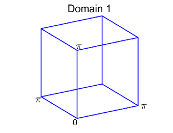
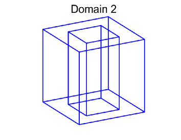
Figure 1: Left: a cubic domain with $[0,\pi]^{3}$. Right: a cubic domain with a hole $[0,\pi]^{3}\setminus[\pi/4,3\pi/4]^{2}\times[0,\pi]$.

We use 5 levels of uniform cubic meshes and their mesh sizes are

$$h=\frac{\pi}{4},\frac{\pi}{8},\frac{\pi}{16},\frac{\pi}{32},\frac{\pi}{64}.$$

For each mesh, the $\mathcal{U}$ in the auxiliary part of the scheme is set to a diagonal matrix

$$\begin{split}\mathcal{U}=\frac{5}{h^{3}}\mathcal{I},\end{split}$$ (55)

where $\mathcal{I}$ is the identity matrix.

The numerical experiments involve many cases including two different operators, both source and eigenvalue problems, two different domains. Moreover, the multigrid method acts both as an independent solver itself and a preconditioner in the Conjugate Gradient (CG) method. To guarantee all these cases to converge, we choose symmetric Gauss-Seidel method as the smoother and set the number of smoothing iteration to $5$ uniformly, even though the these settings are not optimal for every case. We generate the SAIT preconditioner based on the triangular factors of the standard ILU(0) factorization. We also take a uniform setting for the parameters in Algorithm 3, say SAIT$(0.05,10)$.

We use the Locally Optimal Block Preconditioned Conjugate Gradient methd (LOBPCG) [18] as the basic solver to compute the first $20$ eigenvalues of the auxiliary eigenvalue problems. We compute $25$ eigenvalue in actual computations to make the solver stabler. When the errors of first $20$ numerical eigenvalue reach the error criterion, we stop the iteration.

The errors of the linear equations and generalized matrix eigenvalue problems are set as

$$\begin{split}\frac{\|f-\mathscr{A}u\|}{\|f\|}\quad\text{and}\quad\frac{\|\mathscr{A}u-\lambda\mathcal{M}_{k}u\|_{\mathcal{M}_{k}}}{\|u\|_{\mathcal{M}_{k}}},\end{split}$$

respectively. Here, $\|\cdot\|_{\mathcal{M}_{k}}$ denotes the norm with respect to $\mathcal{M}_{k}$, that is

$$\begin{split}\|v\|_{\mathcal{M}_{k}}=\sqrt{v^{T}\mathcal{M}_{k}v}.\end{split}$$

The stop criterion is set to $10^{-8}$ for all the numerical experiments.

6.1 The Maxwell problems

The discrete weak form of the Maxwell source problem (50) is: given $\mathbf{f}\in\mathbf{L}^{2}(\Omega)$, find $\mathbf{u}_{h}\in\mathbf{E}_{h}$ such that

$$\begin{split}\left\langle\nabla\times\mathbf{u}_{h}\,,\,\nabla\times\mathbf{v}_{h}\right\rangle+c\left\langle\mathbf{u}_{h}\,,\,\mathbf{v}_{h}\right\rangle=\left\langle\mathbf{f}\,,\,\mathbf{v}_{h}\right\rangle\quad\mathbf{v}_{h}\in\mathbf{E}_{h}.\end{split}$$ (56)

The corresponding auxiliary weak form is: given $\mathbf{f}\in\mathbf{L}^{2}(\Omega)$, find $(\boldsymbol{\sigma}_{h},\tilde{\mathbf{u}}_{h})\in Q_{h}\times\mathbf{E}_{h}$ such that

$$\begin{split}\left\langle\sigma_{h}\,,\,\tau_{h}\right\rangle-\left\langle\tilde{\mathbf{u}}_{h}\,,\,\nabla\tau_{h}\right\rangle&=0\qquad\qquad\;\,\tau_{h}\in Q_{h},\\ \left\langle\nabla\sigma_{h}\,,\,\mathbf{v}_{h}\right\rangle+\left\langle\nabla\times\tilde{\mathbf{u}}_{h}\,,\,\nabla\times\mathbf{v}_{h}\right\rangle+\left\langle\tilde{\mathbf{u}}_{h}\,,\,\mathbf{v}_{h}\right\rangle&=\left\langle\mathbf{f}\,,\,\mathbf{v}_{h}\right\rangle\;\,\quad\mathbf{v}_{h}\in\mathbf{E}_{h}.\end{split}$$ (57)

The discrete form of Maxwell eigenvalue problem (52) is: find $(\lambda_{h},\mathbf{u}_{h})\in\mathbb{R}\times\mathbf{E}_{h}$ such that

$$\begin{split}\left\langle\nabla\times\mathbf{u}_{h}\,,\,\nabla\times\mathbf{v}_{h}\right\rangle=\lambda_{h}\left\langle\mathbf{u}_{h}\,,\,\mathbf{v}_{h}\right\rangle\quad\mathbf{v}_{h}\in\mathbf{E}_{h}.\end{split}$$ (58)

Its auxiliary problem is: find $(\lambda_{h},\mathbf{u}_{h})\in\mathbb{R}\times\mathbf{E}_{h}$ such that

$$\begin{split}\left\langle\sigma_{h}\,,\,\tau_{h}\right\rangle-\left\langle\tilde{\mathbf{u}}_{h}\,,\,\nabla\tau_{h}\right\rangle&=0\qquad\qquad\qquad\;\,\tau_{h}\in Q_{h},\\ \left\langle\nabla\sigma_{h}\,,\,\mathbf{v}_{h}\right\rangle+\left\langle\nabla\times\tilde{\mathbf{u}}_{h}\,,\,\nabla\times\mathbf{v}_{h}\right\rangle&=\lambda_{h}\left\langle\mathbf{u}_{h}\,,\,\mathbf{v}_{h}\right\rangle\;\,\quad\mathbf{v}_{h}\in\mathbf{E}_{h}.\end{split}$$ (59)

As we discussed in section 4, the mass matrix generated by $\left\langle\sigma_{h}\,,\,\tau_{h}\right\rangle$ in the above auxiliary forms is replace by $\mathbb{U}$ as (55).

Figure 2 shows the comparisons of the nonzero in the lower triangular factor $L$ and its corresponding sparse approximate inverse matrix $M_{L}$ generated by SAIT$(0.05,m)$. Here $m$ is the iteration number in Algorithm 3. The results show that the nonzeros on the SAIT$(0.05,10)$ matrix is much less than its original matrix.

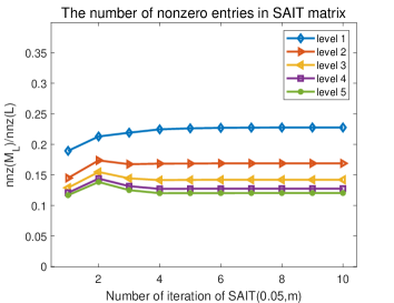
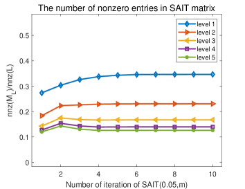
Figure 2: The number of the nonzero entries in the SAIT for the Maxwell equation. Left: Domain 1. Right: Domain 2.

Figure 3 shows the results in solving the original discrete Maxwell equation and its auxiliary problem using the Conjugate Gradient method on the mesh of level 5 ($h=\pi/64$). With the auxiliary part, the convergence becomes stable and faster, and can be accelerated by ILU and SAIT preconditioners further.

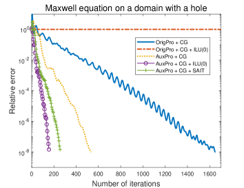
Figure 3: The convergence histories of the original Maxwell equation and the auxiliary scheme with different iterative methods. The mesh is level 5 with the mesh size $h=\pi/64$. Left: Domain 1. Rigth: Domain 2.

After getting the solution of the auxiliary problem, it need to solve a mass equation. Figure 4 shows the relative errors of the mass equation and the original discrete Maxwell problem. The error of the original problem stops going down after some iteration. The reason is that its contains the error in the solution of the auxiliary problem (47) by Theorem 4.5. The figures also show that the relative error of the mass equation is smaller than that of the original equation. This means that the error of the mass euqation should be set smaller in computing.

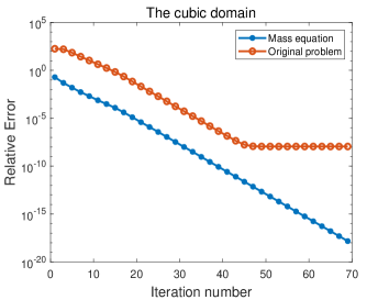
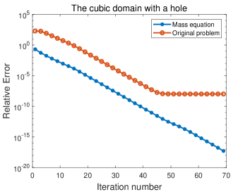
Figure 4: The convergence histories of the mass equation. The relative error is computed in two ways: by the mass equation and by the original discrete Maxwell equation. Left: Domain 1. Rigth: Domain 2.

Table 3 and 4 show more convergence results. The V-cycle multigrid method works both as an independent solver or a preconditioner in the Conjugate Gradient method, and it can reduce the iteration counts significantly. The mass equations on different mesh converge fast even without preconditioning and the ILU(0) can make them converge to the stop criterion within several iterations.

			$(\mathcal{A}+c\mathcal{M}_{k})u=f$		$(\mathcal{A}+\mathcal{B}^{T}\mathcal{U}\mathcal{B}+c\mathcal{M}_{k})u=f$					$\mathcal{M}_{k}u=f$
Level	$h$	d.o.f.	Conjugate Gradient		Conjugate Gradient				Multigrid MGVC$(l,5)$	Conjugate Gradient
			$--$	ILU(0)	$--$	ILU(0)	SAIT	MGVC$(l,5)$		$--$	ILU(0)
$l=1$	$\pi/4$	$300$	$96$	$19$	$64$	$7$	$13$			$15$	$3$
$l=2$	$\pi/8$	$1994$	$208$	$2233$	$84$	$14$	$23$	$8$	$5$	$28$	$3$
$l=3$	$\pi/16$	$13,872$	$395$	$\infty$	$113$	$29$	$48$	$10$	$7$	$32$	$3$
$l=4$	$\pi/32$	$104,544$	$769$	$\infty$	$198$	$60$	$96$	$12$	$10$	$33$	$3$
$l=5$	$\pi/64$	$811,200$	$1544$	$\infty$	$372$	$122$	$191$	$15$	$14$	$33$	$3$

Table 3: The iteration counts of the original discrete Maxwell equation, its auxiliary equation and the mass equation with different iterative methods and preconditioners on Domain 1.

			$(\mathcal{A}+c\mathcal{M}_{k})u=f$		$(\mathcal{A}+\mathcal{B}^{T}\mathcal{U}\mathcal{B}+c\mathcal{M}_{k})u=f$					$\mathcal{M}_{k}u=f$
Level	$h$	d.o.f.	Conjugate Gradient		Conjugate Gradient				Multigrid MGVC$(l,5)$	Conjugate Gradient
			$--$	ILU(0)	$--$	ILU(0)	SAIT	MGVC$(l,5)$		$--$	ILU(0)
$l=1$	$\pi/4$	$276$	$106$	$20$	$64$	$9$	$11$			$28$	$6$
$l=2$	$\pi/8$	$1,656$	$219$	$136$	$93$	$16$	$30$	$5$	$6$	$35$	$7$
$l=3$	$\pi/16$	$11,184$	$416$	$\infty$	$158$	$36$	$57$	$6$	$7$	$36$	$3$
$l=4$	$\pi/32$	$81,504$	$820$	$\infty$	$288$	$78$	$115$	$9$	$11$	$34$	$5$
$l=5$	$\pi/64$	$620,736$	$1643$	$\infty$	$321$	$157$	$235$	$12$	$16$	$33$	$5$

Table 4: The iteration counts of the original discrete Maxwell equation, its auxiliary equation and the mass equation with different iterative methods and preconditioners on Domain 2.

We compute the auxiliary Maxwell eigenvalue problem using LOBPCG method with different preconditioners. Figure 5 shows the convergence histories of the first 20 eigenvalues on Domain 1 with the mesh of level 5 ($h=\pi/64$). All of the ILU(0), SAIT$(0.05,10)$ and MGVC$(l,5)$ preconditioners can efficiently reduce the iteration counts. After getting the eigenpairs of the auxiliary problems, we recompute the numerical eigenvalue using the eigenvectors and the original and the auxiliary operator. Table 5 shows that the smallest nonzero eigenvalues can be easily recognized through recomputing. Table 6 show the eigenvalues on Domain 2 with the mesh of level 5 ($h=\pi/64$). As there is a hole in this domain, the Betti number is $1$. The first eigenpair in this auxiliary eigenvalue problem corresponds to the only one harmonic form in the cohomology space. Table 7 and 8 show the convergence of the auxiliary eigenvalue problem on different meshes.

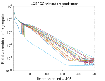
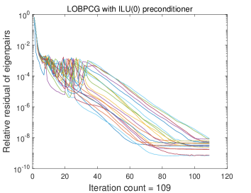
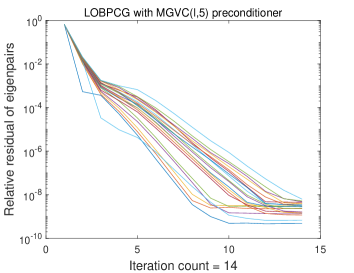
Figure 5: Compute the first 20 eigenvalue of the auxiliary discrete Maxwell operator on Domain 1 with the mesh of level 5 ($h=\frac{\pi}{64}$) using LOBPCG method with ILU(0), SAIT$(0.05,10)$, Multigrid preconditioner, respectively.

Exact	$\left(\mathcal{A}+\mathcal{B}^{T}\mathcal{U}\mathcal{B}\right)u=\lambda_{h}\mathcal{M}_{k}u$	$\mathcal{A}u=\lambda_{h}\mathcal{M}_{k}u$	$\mathcal{B}^{T}\mathcal{U}\mathcal{B}u=\lambda_{h}\mathcal{M}_{k}u$	Type
2	2.000401	2.000401	2.781$\times 10^{-14}$	Type 1
2	2.000401	2.000401	5.524$\times 10^{-13}$	Type 1
2	2.000401	2.000401	1.081$\times 10^{-12}$	Type 1
3	3.000602	3.000602	1.859$\times 10^{-13}$	Type 1
3	3.000602	3.000602	8.440$\times 10^{-13}$	Type 1
	4.696564	1.112$\times 10^{-12}$	4.696564	Type 2
	4.696564	2.115$\times 10^{-12}$	4.696564	Type 2
	4.696564	5.233$\times 10^{-12}$	4.696564	Type 2
5	5.003414	5.003414	9.978$\times 10^{-14}$	Type 1
5	5.003414	5.003414	1.792$\times 10^{-13}$	Type 1
5	5.003414	5.003414	1.851$\times 10^{-13}$	Type 1
5	5.003414	5.003414	3.573$\times 10^{-13}$	Type 1
5	5.003414	5.003414	1.213$\times 10^{-12}$	Type 1
5	5.003414	5.003414	2.020$\times 10^{-12}$	Type 1
6	6.003615	6.003615	2.552$\times 10^{-12}$	Type 1
6	6.003615	6.003615	1.438$\times 10^{-12}$	Type 1
6	6.003615	6.003615	1.405$\times 10^{-12}$	Type 1
6	6.003615	6.003615	1.995$\times 10^{-12}$	Type 1
6	6.003615	6.003615	2.526$\times 10^{-12}$	Type 1
6	6.003615	6.003615	3.177$\times 10^{-12}$	Type 1

Table 5: Recompute the numerical eigenvalues using the original discrete Maxwell operator and the auxiliary operator, respectively(Domian 1).

$\left(\mathcal{A}+\mathcal{B}^{T}\mathcal{U}\mathcal{B}\right)u=\lambda_{h}\mathcal{M}_{k}u$	$\mathcal{A}u=\lambda_{h}\mathcal{M}_{k}u$	$\mathcal{B}^{T}\mathcal{U}\mathcal{B}u=\lambda_{h}\mathcal{M}_{k}u$	Type
5.247$\times 10^{-12}$	4.816$\times 10^{-12}$	4.970$\times 10^{-13}$	Type 0
1.000200	1.000200	9.858$\times 10^{-13}$	Type 1
1.513696	1.513696	5.930$\times 10^{-13}$	Type 1
1.513696	1.513696	7.567$\times 10^{-13}$	Type 1
2.375882	1.761$\times 10^{-12}$	2.375882	Type 2
2.375882	7.735$\times 10^{-12}$	2.375882	Type 2
2.689091	2.689091	2.327$\times 10^{-12}$	Type 1
3.400482	3.400482	4.662$\times 10^{-13}$	Type 1
4.003213	4.003213	5.860$\times 10^{-13}$	Type 1
4.516709	4.516709	5.356$\times 10^{-13}$	Type 1
4.516709	4.516709	2.487$\times 10^{-12}$	Type 1
4.560227	3.255$\times 10^{-12}$	4.560227	Type 2
5.230621	5.230621	5.764$\times 10^{-13}$	Type 1
5.230621	5.230621	1.424$\times 10^{-12}$	Type 1
5.692104	5.692104	1.917$\times 10^{-13}$	Type 1
6.403495	6.403495	6.314$\times 10^{-13}$	Type 1
6.734557	6.734557	4.218$\times 10^{-12}$	Type 1
6.891325	2.839$\times 10^{-11}$	6.891325	Type 2
6.891325	9.671$\times 10^{-11}$	6.891325	Type 2
7.760096	6.702$\times 10^{-11}$	7.760096	Type 2

Table 6: Recompute the numerical eigenvalues using the original discrete Maxwell operator and the auxiliary operator, respectively(Domian 2).

Level	$h$	d.o.f.	LOBPCG with preconditioners
			—	ILU(0)	SAIT(0.05,10)	MGVC(l,5)
$l=1$	$\pi/4$	$300$	$90$	$19$	$23$	$18$
$l=2$	$\pi/8$	$1,944$	$131$	$17$	$29$	$17$
$l=3$	$\pi/16$	$13,872$	$182$	$26$	$54$	$16$
$l=4$	$\pi/32$	$104,544$	$281$	$56$	$107$	$15$
$l=5$	$\pi/64$	$811,200$	$642$	$109$	$211$	$14$

Table 7: The iteration counts in computing the first 20 eigenvalues of the auxiliary Maxwell operator using different preconditioners and different mesh sizes on Domain 1.

Level	$h$	d.o.f.	LOBPCG with preconditioners
			—	ILU(0)	SAIT(0.05,10)	MGVC(l,5)
$l=1$	$\pi/4$	$276$	$83$	$22$	$25$	$21$
$l=2$	$\pi/8$	$1,656$	$135$	$18$	$30$	$18$
$l=3$	$\pi/16$	$11,184$	$161$	$24$	$45$	$15$
$l=4$	$\pi/32$	$81,504$	$257$	$61$	$96$	$14$
$l=5$	$\pi/64$	$620,736$	$484$	$111$	$215$	$14$

Table 8: The iteration counts in computing the first 20 eigenvalues of the auxiliary Maxwell operator using different preconditioners and different mesh sizes on Domain 2.

6.2 The grad-div problems

The discrete weak formulation of the grad-div source problem (51) is: given $\mathbf{f}\in\mathbf{L}^{2}(\Omega)$, find $\mathbf{u}_{h}\in\mathbf{F}_{h}$ such that

$$\begin{split}\left\langle\nabla\cdot\mathbf{u}_{h}\,,\,\nabla\cdot\mathbf{v}_{h}\right\rangle+\left\langle\mathbf{u}_{h}\,,\,\mathbf{v}_{h}\right\rangle=\left\langle\mathbf{f}\,,\,\mathbf{v}_{h}\right\rangle\quad\mathbf{v}_{h}\in\mathbf{F}_{h}.\end{split}$$ (60)

Its auxiliary weak form is: given $\mathbf{f}\in\mathbf{L}^{2}(\Omega)$, find $(\boldsymbol{\sigma}_{h},\tilde{\mathbf{u}}_{h})\in\mathbf{E}_{h}\times\mathbf{F}_{h}$ such that

$$\begin{split}\left\langle\boldsymbol{\sigma}_{h}\,,\,\boldsymbol{\tau}_{h}\right\rangle-\left\langle\tilde{\mathbf{u}}_{h}\,,\,\nabla\times\boldsymbol{\tau}_{h}\right\rangle&=0\qquad\qquad\,\boldsymbol{\tau}_{h}\in\mathbf{E}_{h},\\ \left\langle\nabla\times\boldsymbol{\sigma}_{h}\,,\,\mathbf{v}_{h}\right\rangle+\left\langle\nabla\cdot\tilde{\mathbf{u}}_{h}\,,\,\nabla\cdot\mathbf{v}_{h}\right\rangle+\left\langle\tilde{\mathbf{u}}_{h}\,,\,\mathbf{v}_{h}\right\rangle&=\left\langle\mathbf{f}\,,\,\mathbf{v}_{h}\right\rangle\;\,\quad\mathbf{v}_{h}\in\mathbf{F}_{h}.\end{split}$$ (61)

The discrete weak form the grad-div eigenvalue problem (53) is: find $(\lambda_{h},\mathbf{u}_{h})\in\mathbb{R}\times\mathbf{F}_{h}$ such that

$$\begin{split}\left\langle\nabla\cdot\mathbf{u}_{h}\,,\,\nabla\cdot\mathbf{v}_{h}\right\rangle+c\left\langle\mathbf{u}_{h}\,,\,\mathbf{v}_{h}\right\rangle=\lambda_{h}\left\langle\mathbf{u}_{h}\,,\,\mathbf{v}_{h}\right\rangle\quad\mathbf{v}_{h}\in\mathbf{F}_{h}.\end{split}$$ (62)

Its auxiliary problem is: find $(\lambda_{h},\mathbf{u}_{h})\in\mathbb{R}\times\mathbf{F}_{h}$ such that

$$\begin{split}\left\langle\boldsymbol{\sigma}_{h}\,,\,\boldsymbol{\tau}_{h}\right\rangle-\left\langle\tilde{\mathbf{u}}_{h}\,,\,\nabla\times\boldsymbol{\tau}_{h}\right\rangle&=0\qquad\qquad\qquad\,\boldsymbol{\tau}_{h}\in\mathbf{E}_{h},\\ \left\langle\nabla\times\boldsymbol{\sigma}_{h}\,,\,\mathbf{v}_{h}\right\rangle+\left\langle\nabla\cdot\tilde{\mathbf{u}}_{h}\,,\,\nabla\cdot\mathbf{v}_{h}\right\rangle&=\lambda_{h}\left\langle\mathbf{u}_{h}\,,\,\mathbf{v}_{h}\right\rangle\;\,\quad\mathbf{v}_{h}\in\mathbf{F}_{h}.\end{split}$$ (63)

Most of the results in computing the grad-div problems using auxiliary schemes are similar to those of Maxwell problems. Figure 6 is the nonzero entries in SAIT matrices on different meshes and domains. Figure 7 shows the comparisons of the convergences of the auxiliary grad-div source problem and original problem. The difference from Maxwell case is that ILU(0) works for the original grad-div problem though it doesn’t improve the convergence. Table 9 and 10 show the convergence results on the two domains with different levels of meshes, respectively.

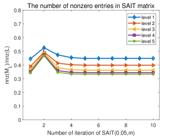
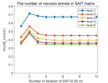
Figure 6: The number of the nonzero entries in the SAIT for the grad-div equation. Left: Domain 1. Right: Domain 2.

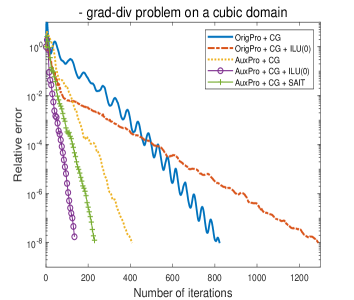
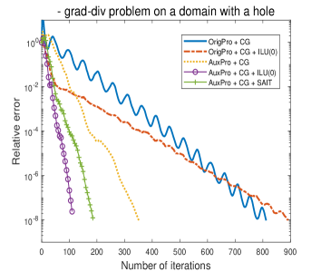
Figure 7: The convergence histories of the original grad-div equation and the auxiliary scheme with different iterative methods. The mesh is level 5 with the mesh size $h=\pi/64$. Left: Domain 1. Rigth: Domain 2.

			$(\mathcal{A}+c\mathcal{M}_{k})u=f$		$(\mathcal{A}+\mathcal{B}^{T}\mathcal{U}\mathcal{B}+c\mathcal{M}_{k})u=f$					$\mathcal{M}_{k}u=f$
Level	$h$	d.o.f.	Conjugate Gradient		Conjugate Gradient				Multigrid MGVC$(l,5)$	Conjugate Gradient
			$--$	ILU(0)	$--$	ILU(0)	SAIT	MGVC$(l,5)$		$--$	ILU(0)
$l=1$	$\pi/4$	$240$	$36$	$19$	$37$	$10$	$15$			$5$	$1$
$l=2$	$\pi/8$	$1,728$	$99$	$45$	$64$	$49$	$29$	$4$	$5$	$9$	$1$
$l=3$	$\pi/16$	$13,056$	$198$	$133$	$112$	$36$	$57$	$6$	$7$	$9$	$1$
$l=4$	$\pi/32$	$101,376$	$406$	$398$	$213$	$70$	$118$	$9$	$10$	$15$	$1$
$l=5$	$\pi/64$	$798,720$	$820$	$1297$	$407$	$138$	$233$	$11$	$15$	$15$	$1$

Table 9: The iteration counts of the original discrete grad-div equation, its auxiliary equation and the mass equation with different iterative methods and preconditioners on Domain 1.

			$(\mathcal{A}+c\mathcal{M}_{k})u=f$		$(\mathcal{A}+\mathcal{B}^{T}\mathcal{U}\mathcal{B}+c\mathcal{M}_{k})u=f$					$\mathcal{M}_{k}u=f$
Level	$h$	d.o.f.	Conjugate Gradient		Conjugate Gradient				Multigrid MGVC$(l,5)$	Conjugate Gradient
			$--$	ILU(0)	$--$	ILU(0)	SAIT	MGVC		$--$	ILU(0)
$l=1$	$\pi/4$	$204$	$55$	$17$	$45$	$10$	$14$			$6$	$1$
$l=2$	$\pi/8$	$1,392$	$109$	$36$	$68$	$17$	$27$	$4$	$6$	$12$	$1$
$l=3$	$\pi/16$	$10,176$	$211$	$103$	$111$	$31$	$48$	$6$	$6$	$17$	$1$
$l=4$	$\pi/32$	$77,568$	$401$	$295$	$197$	$59$	$94$	$7$	$9$	$16$	$1$
$l=5$	$\pi/64$	$605,184$	$816$	$884$	$365$	$113$	$186$	$10$	$13$	$15$	$1$

Table 10: The iteration counts of the original discrete grad-div equation, its auxiliary equation and the mass equation with different iterative methods and preconditioners on Domain 2.

Table 11 and 12 show the results in recomputing the numerical eigenvalues using the original discrete eigenvalue problem (62). Table 14 and 13 show more convergence results of auxiliary discrete grad-div source problem (63) on the two domains, respectively.

Exact	$\left(\mathcal{A}+\mathcal{B}^{T}\mathcal{U}\mathcal{B}\right)u=\lambda_{h}\mathcal{M}_{k}u$	$\mathcal{A}u=\lambda_{h}\mathcal{M}_{k}u$	$\mathcal{B}^{T}\mathcal{U}\mathcal{B}u=\lambda_{h}\mathcal{M}_{k}u$	Type
3	3.000602	3.000602	7.452 $\times 10^{-13}$	Type 1
6	6.003615	6.003615	4.122 $\times 10^{-13}$	Type 1
6	6.003615	6.003615	1.045 $\times 10^{-12}$	Type 1
6	6.003615	6.003615	1.128 $\times 10^{-12}$	Type 1
9	9.006628	9.006628	5.124 $\times 10^{-13}$	Type 1
9	9.006628	9.006628	8.570 $\times 10^{-13}$	Type 1
9	9.006628	9.006628	1.369 $\times 10^{-12}$	Type 1
	9.539861	1.242 $\times 10^{-12}$	9.539861	Type 2
	9.539861	1.989 $\times 10^{-12}$	9.539861	Type 2
	9.539861	3.823 $\times 10^{-12}$	9.539861	Type 2
11	11.016677	11.016677	1.086 $\times 10^{-12}$	Type 1
11	11.016677	11.016677	1.373 $\times 10^{-12}$	Type 1
11	11.016677	11.016677	3.347 $\times 10^{-12}$	Type 1
12	12.009641	12.009641	8.625 $\times 10^{-13}$	Type 1
14	14.019690	14.019690	2.515 $\times 10^{-13}$	Type 1
14	14.019690	14.019690	9.587 $\times 10^{-13}$	Type 1
14	14.019690	14.019690	2.729 $\times 10^{-12}$	Type 1
14	14.019690	14.019690	6.097 $\times 10^{-12}$	Type 1
14	14.019690	14.019690	4.431 $\times 10^{-12}$	Type 1
14	14.019690	14.019690	1.004 $\times 10^{-13}$	Type 1

Table 11: Recompute the numerical eigenvalues using the original discrete grad-div operator and the auxiliary operator, respectively(Domian 1).

$\left(\mathcal{A}+\mathcal{B}^{T}\mathcal{U}\mathcal{B}\right)u=\lambda_{h}\mathcal{M}_{k}u$	$\mathcal{A}u=\lambda_{h}\mathcal{M}_{k}u$	$\mathcal{B}^{T}\mathcal{U}\mathcal{B}u=\lambda_{h}\mathcal{M}_{k}u$	Type
4.533215	4.856 $\times 10^{-12}$	4.533215	Type 2
6.952396	1.882 $\times 10^{-12}$	6.952396	Type 2
6.952396	2.652 $\times 10^{-12}$	6.952396	Type 2
12.455297	3.875 $\times 10^{-13}$	12.455297	Type 2
15.488922	15.488922	4.132 $\times 10^{-13}$	Type 1
15.805105	5.086 $\times 10^{-13}$	15.805105	Type 2
15.921176	15.921176	5.413 $\times 10^{-13}$	Type 1
15.921176	15.921176	4.822 $\times 10^{-13}$	Type 1
16.618025	16.618025	1.017 $\times 10^{-13}$	Type 1
18.109571	7.399 $\times 10^{-13}$	18.109571	Type 2
18.491935	18.491935	4.263 $\times 10^{-13}$	Type 1
18.924189	18.924189	3.922 $\times 10^{-13}$	Type 1
18.924189	18.924189	6.295 $\times 10^{-13}$	Type 1
19.251186	19.251186	2.779 $\times 10^{-13}$	Type 1
19.621038	19.621038	1.210 $\times 10^{-12}$	Type 1
20.546486	1.087 $\times 10^{-12}$	20.546486	Type 2
20.546486	2.856 $\times 10^{-12}$	20.546486	Type 2
20.932342	20.932342	1.935 $\times 10^{-12}$	Type 1
20.932342	20.932342	3.757 $\times 10^{-12}$	Type 1
22.254199	22.254199	1.524 $\times 10^{-09}$	Type 1

Table 12: Recompute the numerical eigenvalues using the original discrete grad-div operator and the auxiliary operator, respectively(Domian 2).

Level	$h$	d.o.f.	LOBPCG with preconditioners
			$--$	ILU(0)	SAIT(0.05,10)	MGVC(l,5)
$l=1$	$\pi/4$	$240$	$83$	$26$	$30$	$25$
$l=2$	$\pi/8$	$1,728$	$167$	$39$	$57$	$34$
$l=3$	$\pi/16$	$13,056$	$175$	$42$	$67$	$18$
$l=4$	$\pi/32$	$101,376$	$303$	$78$	$132$	$17$
$l=5$	$\pi/64$	$798,720$	$655$	$167$	$305$	$17$

Table 13: The iteration counts in computing the first 20 eigenvalues of the auxiliary grad-div operator using different preconditioners and different mesh sizes on Domain 1.

Level	$h$	d.o.f.	LOBPCG with preconditioners
			—	ILU(0)	SAIT(0.05,10)	MGVC(l,5)
$l=1$	$\pi/4$	$204$	$75$	$23$	$25$	$22$
$l=2$	$\pi/8$	$1,392$	$168$	$40$	$52$	$37$
$l=3$	$\pi/16$	$10,176$	$179$	$40$	$65$	$22$
$l=4$	$\pi/32$	$77,568$	$451$	$92$	$141$	$23$
$l=5$	$\pi/64$	$605,184$	$739$	$187$	$269$	$22$

Table 14: The iteration counts in computing the first 20 eigenvalues of the auxiliary grad-div operator using different preconditioners and different mesh sizes on Domain 2.

7 Conclusions

In this paper, we construct auxiliary iterative schemes for the operator $d^{*}d$ using the Hodge Laplacian. The auxiliary schemes are easy to implement using the finite element spaces on the corresponding finite element complex. If the complex is Fredholm, the auxiliary part complements the huge kernel contained in the discrete operator of $d^{*}d$. Then the distribution of the spectrum of the auxiliary problems become Laplace-like. Many iterative methods and preconditioning techniques that are efficient for Laplace operator are also efficient for the auxiliary operator with some simple modifications. The auxiliary schemes of both the source and eigenvalue problems can be computed almost in the same way of Laplace problems. After obtaining the solutions of the auxiliary problems, the desired solutions can be recovered or recognized easily.

We present the Maxwell and grad-div operator on as examples to verify the performance of the auxiliary scheme. We use the ILU method and geometric multigrid method as preconditioning to solve these problems. The numerical tests are all three-dimensional and include various cases, source problems and eigenvalue problems, convex and non-convex domains, different iterative methods and preconditioners. These tests show the efficiency of the new frameworks.

References

- [1] Douglas N. Arnold. Finite element exterior calculus. SIAM, 2018.
- [2] Douglas N. Arnold, Richard S. Falk, and Ragnar Winther. Multigrid in H(div) and H(curl). Numerische Mathematik, 85(2):197–217, 2000.
- [3] Douglas N. Arnold, Richard S. Falk, and Ragnar Winther. Finite element exterior calculus, homological techniques, and applications. Acta Numerica, pages 1–155, 2006.
- [4] Douglas N. Arnold, Richard S. Falk, and Ragnar Winther. Finite element exterior calculus: from hodge theory to numerical stability. Bulletin of the American mathematical society, 47(2):281–354, 2010.
- [5] Zhaojun Bai, James Demmel, Jack Dongarra, Axel Ruhe, and Henk van der Vorst. Templates for the Solution of Algebraic Eigenvalue Problems: A Practical Guide (Software, Environments and Tools). SIAM, 2000.
- [6] Daniele Boffi. Finite element approximation of eigenvalue problems. Acta Numerica, 19:1–120, 2010.
- [7] Daniele Boffi, Franco Brezzi, and Michel Fortin. Mixed Finite Element Methods and Applications, volume 44. Springer, 2013.
- [8] Daniele Boffi, Franco Brezzi, and Lucia Gastaldi. On the convergence of eigenvalues for mixed formulations. Annali della Scuola Normale Superiore di Pisa-Classe di Scienze, 25(1-2):131–154, 1997.
- [9] Daniele Boffi, Franco Brezzi, and Lucia Gastaldi. On the problem of spurious eigenvalues in the approximation of linear elliptic problems in mixed form. Mathematics of Computation, 69(229):121–140, 2000.
- [10] Daniele Boffi, Zhongjie Lu, and Luca F. Pavarino. Iterative ILU preconditioners for linear systems and eigenproblems. Journal of Computational Mathematics, to appear.
- [11] Anne Greenbaum. Iterative methods for solving linear systems, volume 17. SIAM, 1997.
- [12] Ralf Hiptmair. Multigrid method for maxwell’s equations. SIAM Journal on Numerical Analysis, 36(1):204–225, 1998.
- [13] Ralf Hiptmair. Finite elements in computational electromagnetism. Acta Numerica, 11:237–339, 2002.
- [14] Ralf Hiptmair and Klaus Neymeyr. Multilevel method for mixed eigenproblems. SIAM Journal on Scientific Computing, 23(6):2141–2164, 2002.
- [15] Ralf Hiptmair and Jinchao Xu. Nodal auxiliary space preconditioning in H(curl) and H(div) spaces. SIAM Journal on Numerical Analysis, 45(6):2483–2509, 2007.
- [16] Fumio Kikuchi. Mixed and penalty formulations for finite element analysis of an eigenvalue problem in electromagnetism. Computer Methods in Applied Mechanics and Engineering, 64(1):509–521, 1987.
- [17] Fumio Kikuchi. On a discrete compactness property for the Nédélec finite elements. Journal of The Faculty of Science, The University of Tokyo, Section IA, Mathematics, 36(3):479–490, 1989.
- [18] Andrew V. Knyazev. Toward the optimal preconditioned eigensolver: Locally optimal block preconditioned conjugate gradient method. SIAM Journal on Scientific Computing, 23(2):517–541, 2001.
- [19] Zhongjie Lu. A sparse approximate inverse for triangular matrices based on Jacobi iteration. submitted.
- [20] Jean-Claude Nédélec. Mixed finite elements in . Numerische Mathematik, 35(3):315–341, 1980.
- [21] Yousef Saad. Iterative methods for sparse linear systems. Society for Industrial and Applied Mathematics, Philadelphia, PA, second edition, 2003.