Matrix Representation of Time-Delay Interferometry

Abstract

Time-Delay Interferometry (TDI) is the data processing technique that cancels the large laser phase fluctuations affecting the one-way Doppler measurements made by unequal-arm space-based gravitational wave interferometers. By taking finite linear combinations of properly time-shifted Doppler measurements, laser phase fluctuations are removed at any time $t$ and gravitational wave signals can be studied at a requisite level of precision.

In this article we show the delay operators used in TDI can be represented as matrices acting on arrays associated with the laser noises and Doppler measurements. The matrix formulation is nothing but the group theoretic representation (ring homomorphism) of the earlier approach involving time-delay operators and so in principle is the same. It is shown that the homomorphism is valid generally and we cover all situations of interest. To understand the potential advantages the matrix representation brings, care must be taken by the data analyst to account for the light travel times when linearly relating the one-way Doppler measurements to the laser noises. This is especially important in view of the future gravitational wave projects envisaged. We show that the matrix formulation of TDI results in the cancellation of the laser noises at an arbitrary time $t$ by only linearly combining a finite number of samples of the one-way Doppler data measured at and around time $t$.

I Introduction

Interferometric detectors of gravitational waves with frequency content $0<f<f_{0}$ may be thought of as optical configurations with one or more arms folding coherent trains of electromagnetic waves (or beams) of nominal frequency $\nu_{0}\gg f_{0}$. At points where these intersect, relative fluctuations of frequency or phase are monitored (homodyne detection). Frequency fluctuations in a narrow Fourier band can alternatively be described as fluctuating side-band amplitudes. Interference of two or more beams, produced and monitored by a (nonlinear) device such as a photo detector, exhibits these side-bands as a low frequency signal again with frequency content $0<f<f_{0}$. The observed low frequency signal is due to frequency variations of the sources of the beams about $\nu_{0}$, to relative motions of the sources and any mirrors (or amplifying microwave or optical transponders) that do any beam folding, to temporal variations of the index of refraction along the beams, and, according to general relativity, to any time-variable gravitational fields present, such as the transverse trace-less metric curvature of a passing plane gravitational wave train. To observe these gravitational fields in this way, it is thus necessary to control, or monitor, the other sources of relative frequency fluctuations, and, in the data analysis, to optimally use algorithms based on the different characteristic interferometer responses to gravitational waves (the signal) and to the other sources (the noise).

By comparing phases of split beams propagated along equal but non-parallel arms, frequency fluctuations from the source of the beams are removed directly at the photo detector and gravitational wave signals at levels many orders of magnitude lower can be detected. Especially for interferometers that use light generated by presently available lasers, which display frequency stability roughly a few parts in $10^{-13}$ in the millihertz band, it is essential to remove these fluctuations when searching for gravitational waves of dimensionless amplitude smaller than $10^{-21}$.

Space-based, two-arm interferometers Amaro-Seoane et al. (2017); Hu and Wu (2017); Luo et al. (2016); Tinto et al. (2015); Ni (2016) are prevented from canceling the laser noise by directly interfering the beams from the two unequal arms at a single photo detector because laser phase fluctuations experience different delays. As a result, two Doppler data from the two arms are measured at two different photo detectors and are then digitally processed to compensate for the inequality of the arms. This data processing technique, called Time-Delay Interferometry (TDI) Tinto and Dhurandhar (2021), entails time-shifting and linearly combining the two Doppler measurements so as to achieve the required sensitivity to gravitational radiation.

In a recent article Vallisneri et al. (2021), a data processing alternative to TDI has been proposed for the two-arm configuration. This technique, which has been named TDI-$\infty$ (as it cancels the laser noise at an arbitrary time $t$ by linearly combining all the Doppler measurements made up to time $t$), relies on an identified linear relationship between the two Doppler measurements made by an unequal-arm Michelson interferometer and the laser noise. Based on this formulation, TDI-$\infty$ cancels laser phase fluctuations by applying linear algebra manipulations to the Doppler data. Through its implementation, TDI-$\infty$ is claimed to (i) simplify the data processing for gravitational wave signal searches in the laser-noise-free data over that of TDI, (ii) work for any time-dependent light-time delays, and (iii) automatically handle data gaps.

After briefly reviewing the TDI-$\infty$ technique for the two unequal-arm configuration, we show care must be taken to account for the light-travel-times when linearly relating the two-way Doppler measurements to the laser noise Vallisneri et al. (2021). The two-way Doppler data at a time $t$ is the result of the interference between the returning beam and the outgoing beam. As such it contains the difference between the value of the laser noise at time $t-l_{i}(t)$ affecting the returning beam (with $l_{i}(t)$ being the round-trip-light-time (RTLT)) and the laser noise of the outgoing beam at time $t$ when the measurement is recorded. From the instant the laser is switched on (let us say $t=0$) each two-way Doppler measurement becomes different from zero only for $t\geq l_{i}(t)$, i.e. when the returning beam and the outgoing beam start to interfere. By accounting for this observation in the “boundary conditions” of the Doppler data, we show that it is possible to introduce a matrix representation of TDI.

We would like to briefly mention here another matrix based approach. Romano and Woan Romano and Woan (2006) have used Bayesian inference to set up a noise covariance matrix of the data streams. Then by performing a principal component analysis of the covariance matrix, they identify the principal components with large eigenvalues with the laser noise and so distinguish it from other ambient noises and signal which correspond to small eigenvalues. We argue that this approach is also a matrix representation of the original TDI.

Here we provide a summary of this article. In section II we present the key-points of TDI-$\infty$ and correct the expression of the matrix introduced in Vallisneri et al. (2021) relating the two arrays associated with the two-way Doppler measurements to the array of the laser noise. We then recast this linear relationship in terms of two square-matrices, each relating the array associated with one of the two-way Doppler measurement to the array of the laser noise. As expected these matrices are singular, reflecting the physical impossibility of reconstructing the laser noise array from the arrays associated with the two-way Doppler data. In the simple configuration of a stationary interferometer whose RTLTs are integer-multiples of the sampling time, we show that the linear combination of the two-way Doppler arrays canceling the laser noise is equal to the sampled unequal-arm Michelson TDI combination $X$. In section III we then turn to the problem of a stationary three-arm array with three laser noises and six one-way Doppler measurements. After deriving the expressions of the matrices relating the laser noises to the one-way Doppler measurements, we show that the generators of the space of the combinations canceling the laser noises are equal to the sampled TDI-combinations ($\alpha,\beta,\gamma,\zeta$) Tinto and Dhurandhar (2021) in which the delay operators have been replaced by our derived matrices. This is rigorously established in section IV by showing that the matrix formulation is just a ring representation of the first module of syzygies - a ring homomorphism. We cover all cases of interest. We first start with delays that are integer multiples of the sampling interval, then the continuum case when the sampling is continuous and the sampling interval tends to zero and finally when fractional-delay filtering based on Lagrange polynomials is used for reconstructing the samples at any required time. For fractional delays we show that homomorphism is valid (i) when all delays lie in the same interpolation interval, (ii) for each delay lying in different interpolation intervals and also (iii) for time-dependent arm-lengths. In all these cases we show that there is a ring homomorphism. Thus the matrix formulation is in principle the same as the original formulation of TDI, although it might offer some advantages when implemented numerically. Finally, in section V we present our concluding remarks and summarize our thoughts about potential advantages in processing the TDI measurements cast in matrix form when searching for gravitational wave signals.

II Matrix representation of the two-way Doppler measurements

Equal-arm interferometer detectors of gravitational waves can observe gravitational radiation by canceling the laser frequency fluctuations affecting the light injected into their arms. This is done by comparing phases of split beams propagated along the equal (but non-parallel) arms of the detector. The laser frequency fluctuations affecting the two beams experience the same delay within the two equal-length arms and cancel out at the photo-detector where relative phases are measured. This way gravitational-wave signals of dimensionless amplitude less than $10^{-22}$ can be observed when using lasers whose frequency stability can be as large as roughly a few parts in $10^{-18}$ in the kilohertz band.

If the arms of the interferometer have different lengths, however, the exact cancellation of the laser frequency fluctuations, say $C(t)$, will no longer take place at the photo-detector. In fact, the larger the difference between the two arms, the larger will be the magnitude of the laser frequency fluctuations affecting the detector response. If $l_{1}$ and $l_{2}$ are the RTLTs of the laser beams within the two arms, it is easy to see that the amount of laser relative frequency fluctuations remaining in the response are equal to:

$$\Delta C(t)=C(t-l_{1})-C(t-l_{2})\,.$$ (1)

In the case of a space-based interferometer such as LISA for instance, whose lasers are expected to display relative frequency fluctuations equal to about $10^{-13}/\sqrt{\mathrm{Hz}}$ in the mHz band and RTLTs will differ by a few percent Amaro-Seoane et al. (2017), Eq. (1) implies uncanceled fluctuations from the laser as large as $\approx 10^{-16}/\sqrt{\mathrm{Hz}}$ at a millihertz frequency Tinto and Dhurandhar (2021). Since the LISA sensitivity goal is about $10^{-20}/\sqrt{\mathrm{Hz}}$ in this part of the frequency band, it is clear that an alternative experimental approach for canceling the laser frequency fluctuations is needed.

An elegant method entirely implemented in the time domain was first suggested in Tinto and Armstrong (1999) and then generalized in a series of related publications (see Tinto and Dhurandhar (2021) and references therein). Such a method, named Time-Delay Interferometry (or TDI) as it requires time-shifting and linearly combining the recorded data, carefully accounts for the time-signature of the laser noise in the two-way Doppler data. TDI relies on the optical configuration exemplified by Fig. 1 Faller and Bender (1984); Faller et al. (1985, 1989); Giampieri et al. (1996). In this idealized model the two beams exiting the two arms are not made to interfere at a common photo-detector. Rather, each is made to interfere with the incoming light from the laser at a photo-detector, decoupling in this way the laser phase fluctuations experienced by the two beams in the two arms. In the case of a stationary array, cancellation of the laser noise at an arbitrary time $t$ requires only four samples of the measurements made at and around $t$. Contrary to a previously proposed technique Faller and Bender (1984); Faller et al. (1985, 1989); Giampieri et al. (1996), which required processing in the Fourier domain a large ($\sim$ six months) amount of data to sufficiently suppress the laser noise at a time $t$ Tinto and Armstrong (1999); Tinto and Dhurandhar (2021), TDI can be regarded as a “local” method.

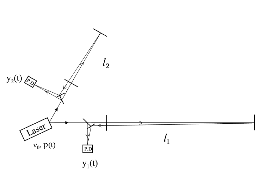
Figure 1: Light from a laser is split into two beams, each injected into an arm formed by pairs of free-falling mirrors. Since the RTLTs, $l_{1}$ and $l_{2}$, are different, now the light beams from the two arms are not recombined at one photo detector. Instead each is separately made to interfere with the light that is injected into the arms. Two distinct photo detectors are now used, and phase (or frequency) fluctuations are then monitored and recorded there.

In a recent publication Vallisneri et al. (2021), a new “global” technique for canceling the laser noise has been proposed. This technique, which has been named TDI-$\infty$, establishes a linear relationship between the sampled Doppler measurements and the laser noise arrays. It is claimed to work for any time-dependent delays and to cancel the laser noise at an arbitrary time $t$ by taking linear combinations of the two-way Doppler measurements sampled at all times before $t$.

To understand the formulation of TDI-$\infty$, let us consider again the simplified (and stationary) two-arm optical configuration shown in Figure 1. In it the laser noise, $C(t)$, folds into the two two-way Doppler data, $y_{1}(t)$, $y_{2}(t)$, in the following way (where we disregard the contributions from all other physical effects affecting the two-way Doppler data):

$$y_{1}(t)=C(t-l_{1}(t))-C(t)\ ,$$

$$y_{2}(t)=C(t-l_{2}(t))-C(t)\ ,$$ (2)

where $l_{1}$, $l_{2}$ are the two RTLTs, in general also functions of time $t$.

Operationally, Eq. (2) says that each sample of the two-way Doppler data at time $t$ contains the difference between the laser noise $C$ generated at a RTLT earlier, $t-l_{i}(t)\ ,\ i=1,2$ and that generated at time $t$. Figure 2 displays graphically what we have just described. The important point to note here is what happens during the first $l_{i}$ seconds from the instant $t=0$ when the laser is switched on. Since the $y_{i}$ measurements are the result of interfering the returned beam with the outgoing one, during the first $l_{i}$ seconds (i.e. from the moment the laser has been turned on) the $y_{i}$ measurements are identically equal to zero because no interference measurements can be performed during this time. In other words, during the first $l_{i}$ seconds there is not yet a returning beam with which the local light is made to interfere with. In Vallisneri et al. (2021), however, only the first terms on the right-hand-sides of Eq. (2) were disregarded during these time intervals. Although the TDI-$\infty$ technique is mathematically correct, by using these nonphysical ”boundary conditions” results in solutions that do not cancel the laser noise when applied to the Doppler data measured by future space-based interferometers. We verified this analytically (by implementing the TDI-$\infty$ algorithm with the help of the program Mathematica Wolfram (2014)) when the two light-times are constant and equal to integer multiples of the sampling time. We found the resulting solutions to be linear combinations of the TDI unequal-arm Michelson combination $X$ defined at each of the sampled times, plus an additional term that would not cancel the laser noise in the measured data. This additional term is a function of $y_{1}$ and $y_{2}$ defined at times $t<l_{1},l_{2}$ and thus, is a manifestation of the non-physical boundary conditions. In the attempt of avoiding this problem one might consider start processing the Doppler data at any time $t$ after the first RTLT has past. However, one would still be confronted by the fact that the Doppler measurement $y_{i}$ at time $t$ contains laser noise generated at time $t$ and at time $t-l_{i}$. In other words, there exists a time-mismatch between the array of the Doppler measurement and that of the laser noise and physical boundary conditions have to be accounted for in a realistic simulation.

TDI-$\infty$ is a “global” data processing algorithm, i.e. its solutions at time $t$ require use of all samples of the Doppler measurements recorded up to time $t$. Our computations for assessing the effects of the nonphysical boundary conditions were carried out only for time intervals relatively short, namely, for stretches of data containing about 200 samples. Although they indicate the dependence of the solutions on the boundary conditions, it is possible that for year-long stretches of data the effects of the selected boundary conditions might not be significant. This, however, needs to be mathematically proved. A detailed mathematical investigation of this point should be carried out in the future and may require extensive work.

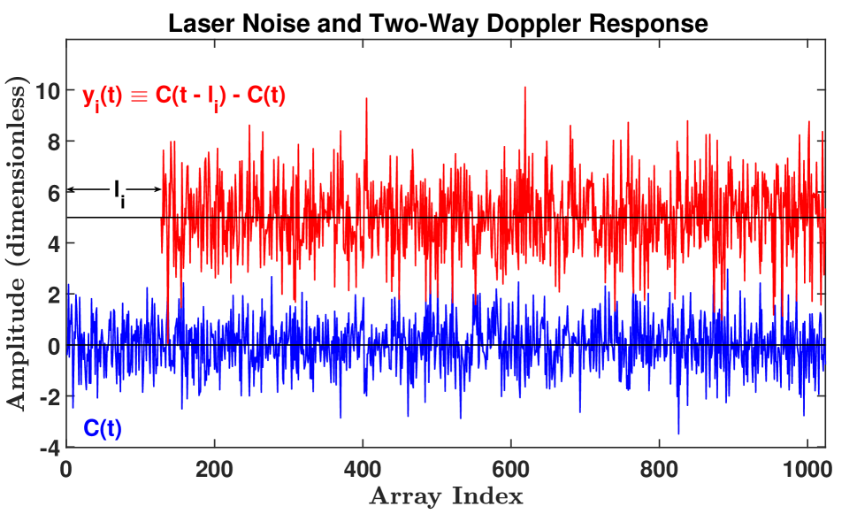
Figure 2: The laser noise random process (blue color), $C(t)$, together with the corresponding two-way Doppler measurement (red color), $y_{i}$. The laser is switched on at time $t=0$. Since it takes $l_{i}$ seconds for the beam to return to the transmitting spacecraft, $y_{i}$ is identically equal to zero since no Doppler measurements can be performed during this time interval.

In TDI-$\infty$ the sampled two two-way Doppler data are packaged in a single array in an alternating fashion starting from time $t=t_{0}$ when the laser is switched on. Assuming a stationary array configuration in which the RTLTs $l_{1}$, $l_{2}$ are equal to twice and three times the sampling time $\Delta t$, (as exemplified in Vallisneri et al. (2021)), the measurements array is linearly related to the array associated with the samples of the laser noise $C$ through a rectangular $2N\times N$ matrix $M$ ($N$ being the number of considered samples) in the following way:

$$\left(\begin{array}[]{c}y_{1}(t_{0})\\ y_{2}(t_{0})\\ y_{1}(t_{1})\\ y_{2}(t_{1})\\ y_{1}(t_{2})\\ y_{2}(t_{2})\\ y_{1}(t_{3})\\ y_{2}(t_{3})\\ y_{1}(t_{4})\\ y_{2}(t_{4})\\ \vdots\end{array}\right)=\left(\begin{array}[]{rrrrrr}-1&0&0&0&0&\cdots\\ -1&0&0&0&0&\cdots\\ 0&-1&0&0&0&\cdots\\ 0&-1&0&0&0&\cdots\\ 1&0&-1&0&0&\cdots\\ 0&0&-1&0&0&\cdots\\ 0&1&0&-1&0&\cdots\\ 1&0&0&-1&0&\cdots\\ 0&0&1&0&-1&\cdots\\ 0&1&0&0&-1&\cdots\\ \vdots&\vdots&\vdots&\vdots&\vdots&\ddots\end{array}\right)\cdot\left(\begin{array}[]{c}c(t_{0})\\ c(t_{1})\\ c(t_{2})\\ c(t_{3})\\ c(t_{4})\\ \vdots\end{array}\right)\ .$$ (3)

As shown by Eq. (3), rows $1$ through $4$ and row $6$ of matrix $M$ reflect the assumption made in Vallisneri et al. (2021) of the two Doppler measurements to contain the laser noise $C$ only at time $t$ during the time intervals $t_{0}\leq t<t_{0}+l_{i}$. If, on the other hand, we correctly assume rows $1$ through $4$ and row $6$ to be identically equal to zero, the null-space associated to the matrix $M$ will clearly be different.

To better understand and quantify this difference, we split the above measurement’s array in two arrays, ($Y_{1},Y_{2}$), (one per measurement) and introduce two corresponding ($N\times N$) square-matrices relating the measurement arrays to the array of the laser noise. We assume again a stationary configuration with RTLTs ($l_{1},l_{2}$) equal to twice and three-times the sampling time respectively. The two vectors, $Y_{1}$, $Y_{2}$, are related to the laser noise vector $C$ through the following expressions:

$$Y_{1}=A_{1}.C\ \ \ ;\ \ \ Y_{2}=A_{2}.C\ ,$$ (4)

where the symbol . denotes matrix multiplication, and $A_{1}$, $A_{2}$ are equal to the following square-matrices:

$$A_{1}=\left(\begin{array}[]{rrrrrrr}0&0&0&0&0&0&\cdots\\ 0&0&0&0&0&0&\cdots\\ 1&0&-1&0&0&0&\cdots\\ 0&1&0&-1&0&0&\cdots\\ 0&0&1&0&-1&0&\cdots\\ 0&0&0&1&0&&-1\cdots\\ \vdots&\vdots&\vdots&\vdots&\vdots&\ddots&\ddots\end{array}\right)\ \ \ \ ,A_{2}=\left(\begin{array}[]{rrrrrrr}0&0&0&0&0&0&\cdots\\ 0&0&0&0&0&0&\cdots\\ 0&0&0&0&0&0&\cdots\\ 1&0&0&-1&0&0&\cdots\\ 0&1&0&0&-1&0&\cdots\\ 0&0&1&0&0&-1&\cdots\\ \vdots&\vdots&\vdots&\vdots&\vdots&\ddots&\ddots\end{array}\right)\ .$$ (5)

Note the above matrices incorporate the correct “boundary conditions” as their first few rows are null (the number of null rows depends on the magnitude of the RTLT). It is evident that the rank of the matrices $A_{1}$, $A_{2}$ is less than the number of samples $N$ and therefore they cannot be inverted. Physically this means that, although the laser noise cannot be known/measured at any time $t$, one can still cancel it by taking suitable linear combinations of the two-way Doppler data. Let us consider the following linear combination of the two-way Doppler measurements:

$$X\equiv A_{2}.Y_{1}-A_{1}.Y_{2}=(A_{2}.A_{1}-A_{1}.A_{2}).C\ .$$ (6)

We have verified that the commutator $[A_{1},A_{2}]$ starts to become zero from row 6 onward. If we write the vectors $Y_{1}$, $Y_{2}$ in terms of their components, the linear combination $X$ becomes equal to:

$$X=\left(\begin{array}[]{c}0\\ 0\\ 0\\ y_{1}(t_{3})-y_{2}(t_{3})\\ y_{1}(t_{4})-y_{2}(t_{4})\\ -y_{1}(t_{2})+y_{1}(t_{5})+y_{2}(t_{3})-y_{2}(t_{5})\\ -y_{1}(t_{3})+y_{1}(t_{6})+y_{2}(t_{4})-y_{2}(t_{6})\\ \vdots\end{array}\right)$$ (7)

The above vector $X$ is no other than the unequal-arm Michelson TDI combination sampled at successive sampling times. Note that $X$ starts to cancel the laser noise after $l_{1}+l_{2}=5\Delta t$ time-samples have past.

If we would incorporate in the matrices $A_{1}$, $A_{2}$ nonphysical “boundary conditions”, they now would be of rank $N$ and therefore invertible. As each Doppler data could be used to reconstruct the laser noise, one could then derive a laser-noise-free combination sensitive to gravitational radiation by taking the difference of the two reconstructions. Since each reconstruction of the laser noise at time $t$ would be a linear combination of samples taken at times determined only by the RTLT of the time-series used, any time-dependence of the RTLT could be accommodated. In other words, since each time-series would not be delayed by the RTLT associated with the other time-series, issues related to the non-commutativity of the delay operators would not be present.

III Matrix Formulation of TDI

In the general case of three arms, we have six one-way Doppler measurements and three independent laser noises. The analysis below will also assume a stationary array and the one-way-light-times to be equal to $L_{1}=\Delta t$, $L_{2}=2\ \Delta t$, $L_{3}=3\ \Delta t$ respectively. Although these RTLTs do not reflect the array’s triangular shape, we adopt them so that we can minimize the size of the matrices introduced for explaining our method without loss of generality.

By generalizing what was described in the previous section for the $X$ combination, we may write the one-way Doppler data in terms of the laser noises in the following form (using the notation introduced in Tinto and Dhurandhar (2021)):

$$y_{1} = D_{3}.C_{2}-I_{3}.C_{1}\ \ ,\ \ y_{1^{\prime}}=D_{2}.C_{3}-I_{2}.C_{1}$$

$$y_{2} = D_{1}.C_{3}-I_{1}.C_{2}\ \ ,\ \ y_{2^{\prime}}=D_{3}.C_{1}-I_{3}.C_{2}$$

$$y_{3} = D_{2}.C_{1}-I_{2}.C_{3}\ \ ,\ \ y_{3^{\prime}}=D_{1}.C_{2}-I_{1}.C_{3}$$ (8)

In Eq.(8) we index the one-way Doppler data as follows: the beam arriving at spacecraft $i$ has subscript $i$ and is primed or unprimed depending on whether the beam is traveling clockwise or counter-clockwise around the interferometer array, with the sense defined by a chosen orientation of the array; the matrices $D_{i}$ correspond to the delay operators of TDI and there are only three of them because the array is stationary Tinto and Dhurandhar (2021). The expressions for $D_{i}$ and $I_{i}$ are equal to:

$$D_{3}=\left(\begin{array}[]{rrrrrrrr}0&0&0&0&0&0&0&\cdots\\ 0&0&0&0&0&0&0&\cdots\\ 0&0&0&0&0&0&0&\cdots\\ 1&0&0&0&0&0&0&\cdots\\ 0&1&0&0&0&0&0&\cdots\\ 0&0&1&0&0&0&0&\cdots\\ 0&0&0&1&0&0&0&\cdots\\ \vdots&\vdots&\vdots&\vdots&\vdots&\vdots&\vdots&\ddots\end{array}\right)\ \ \ \ ,I_{3}=\left(\begin{array}[]{rrrrrrrr}0&0&0&0&0&0&0&\cdots\\ 0&0&0&0&0&0&0&\cdots\\ 0&0&0&0&0&0&0&\cdots\\ 0&0&0&1&0&0&0&\cdots\\ 0&0&0&0&1&0&0&\cdots\\ 0&0&0&0&0&1&0&\cdots\\ 0&0&0&0&0&0&1&\cdots\\ \vdots&\vdots&\vdots&\vdots&\vdots&\vdots&\vdots&\ddots\end{array}\right)\ ;$$ (9)

$$D_{2}=\left(\begin{array}[]{rrrrrrrr}0&0&0&0&0&0&0&\cdots\\ 0&0&0&0&0&0&0&\cdots\\ 1&0&0&0&0&0&0&\cdots\\ 0&1&0&0&0&0&0&\cdots\\ 0&0&1&0&0&0&0&\cdots\\ 0&0&0&1&0&0&0&\cdots\\ 0&0&0&0&1&0&0&\cdots\\ \vdots&\vdots&\vdots&\vdots&\vdots&\vdots&\vdots&\ddots\end{array}\right)\ \ \ \ ,I_{2}=\left(\begin{array}[]{rrrrrrrr}0&0&0&0&0&0&0&\cdots\\ 0&0&0&0&0&0&0&\cdots\\ 0&0&1&0&0&0&0&\cdots\\ 0&0&0&1&0&0&0&\cdots\\ 0&0&0&0&1&0&0&\cdots\\ 0&0&0&0&0&1&0&\cdots\\ 0&0&0&0&0&0&1&\cdots\\ \vdots&\vdots&\vdots&\vdots&\vdots&\vdots&\vdots&\ddots\end{array}\right)\ ;$$ (10)

$$D_{1}=\left(\begin{array}[]{rrrrrrrr}0&0&0&0&0&0&0&\cdots\\ 1&0&0&0&0&0&0&\cdots\\ 0&1&0&0&0&0&0&\cdots\\ 0&0&1&0&0&0&0&\cdots\\ 0&0&0&1&0&0&0&\cdots\\ 0&0&0&0&1&0&0&\cdots\\ 0&0&0&0&0&1&0&\cdots\\ \vdots&\vdots&\vdots&\vdots&\vdots&\vdots&\vdots&\ddots\end{array}\right)\ \ \ \ ,I_{1}=\left(\begin{array}[]{rrrrrrrr}0&0&0&0&0&0&0&\cdots\\ 0&1&0&0&0&0&0&\cdots\\ 0&0&1&0&0&0&0&\cdots\\ 0&0&0&1&0&0&0&\cdots\\ 0&0&0&0&1&0&0&\cdots\\ 0&0&0&0&0&1&0&\cdots\\ 0&0&0&0&0&0&1&\cdots\\ \vdots&\vdots&\vdots&\vdots&\vdots&\vdots&\vdots&\ddots\end{array}\right)\ .$$ (11)

The problem of identifying all possible TDI combinations associated with the six one-way Doppler measurements becomes one of determining six matrices, $q_{i},q_{i^{\prime}}$ such that the following equation holds:

$$\sum_{i=1}^{3}q_{i}.y_{i}+\sum_{i^{\prime}=1}^{3}q_{i^{\prime}}.y_{i^{\prime}}=0\ ,$$ (12)

where the above equality means “zero laser noises”. Before proceeding, note that the matrices $D_{i}$ and $I_{i}$ satisfy the following identities which may be useful later on:

$$I_{i}.D_{k} = D_{k}\,,~{}~{}~{}~{}~{}i\leq k$$

$$\neq D_{k}\,,~{}~{}~{}~{}~{}~{}i>k$$

$$I_{i}.I_{k} = I_{k}.I_{i}=I_{k}\,,~{}~{}~{}~{}~{}~{}~{}i\leq k\,.$$ (13)

The above identities in particular state that $I_{k}^{2}=I_{k}$, that is, $I_{k}$ are idempotent, or in other words they are projection operators.

By redefining the matrices $q_{i}$, $q_{i^{\prime}}$ in the following way:

$$q_{1}.I_{3} \rightarrow q_{1}\ \ ,\ \ q_{2}.I_{1}\rightarrow q_{2}\ \ ,\ \ q_{3}.I_{2}\rightarrow q_{3}\ ,$$

$$q_{1^{\prime}}.I_{2} \rightarrow q_{1^{\prime}}\ \ ,\ \ q_{2^{\prime}}.I_{3}\rightarrow q_{2^{\prime}}\ \ ,\ \ q_{3^{\prime}}.I_{1}\rightarrow q_{3^{\prime}}\ ,$$ (14)

Eq. (12) assumes the following form:

$$( -q_{1}-q_{1^{\prime}}+q_{3}.D_{2}+q_{2^{\prime}}.D_{3}).C_{1}$$

$$+ ( -q_{2}-q_{2^{\prime}}+q_{1}.D_{3}+q_{3^{\prime}}.D_{1}).C_{2}$$

$$+ ( -q_{3}-q_{3^{\prime}}+q_{2}.D_{1}+q_{1^{\prime}}.D_{2}).C_{3}=0$$ (15)

Since the three random processes $C_{i}\ ,\ i=1,2,3$ are independent, the above equation can be satisfied iff the three matrices multiplying the three random processes are identically equal to zero, i.e.:

$$-q_{1}-q_{1^{\prime}}+q_{3}.D_{2}+q_{2^{\prime}}.D_{3}=0\ ,$$

$$-q_{2}-q_{2^{\prime}}+q_{1}.D_{3}+q_{3^{\prime}}.D_{1}=0\ ,$$

$$-q_{3}-q_{3^{\prime}}+q_{2}.D_{1}+q_{1^{\prime}}.D_{2}=0\ .$$ (16)

Since the system of Eqs. (16) is identical in form to the corresponding equations derived in Tinto and Dhurandhar (2021) (see section 4.3 of Tinto and Dhurandhar (2021) and equations therein), the solutions will assume the same forms. It should be noticed, however, that the “matrix” expressions of the generators $\alpha,\beta,\gamma,\zeta$ can be obtained from the usual TDI-expressions by taking into account that the $qs$ had been redefined (see Eq.(14) ). This means that the Sagnac combination $\alpha$, for instance, assumes the following form:

$$\alpha=(y_{1}+D_{3}y_{2}+D_{1}D_{3}y_{3})-(y_{1^{\prime}}+D_{2}y_{3^{\prime}}+D_{1}D_{2}y_{2^{\prime}})\ ,$$ (17)

where we have accounted for the identities given by Eqs. (13). When considering seven time-samples of the six one-way measurements, the above expression for $\alpha$ reduces to the following vector:

$$\alpha=\left(\begin{array}[]{c}0\\ 0\\ -y_{1^{\prime}}(t_{2})-y_{3^{\prime}}(t_{0})\\ y_{1}(t_{3})-y_{1^{\prime}}(t_{3})+y_{2}(t_{0})-y_{2^{\prime}}(t_{0})-y_{3^{\prime}}(t_{1})\\ y_{1}(t_{4})-y_{1^{\prime}}(t_{4})+y_{2}(t_{1})-y_{2^{\prime}}(t_{1})+y_{3}(t_{0})-y_{3^{\prime}}(t_{2})\\ y_{1}(t_{5})-y_{1^{\prime}}(t_{5})+y_{2}(t_{2})-y_{2^{\prime}}(t_{2})+y_{3}(t_{1})-y_{3^{\prime}}(t_{3})\\ y_{1}(t_{6})-y_{1^{\prime}}(t_{6})+y_{2}(t_{3})-y_{2^{\prime}}(t_{3})+y_{3}(t_{2})-y_{3^{\prime}}(t_{4})\\ \vdots\end{array}\right)$$ (18)

As in the case of the combination $X$ presented in the previous section, here also the first few entries of the vector cannot cancel the laser noises. This is because some of the measurements at those time stamps are equal to zero. However, it is easy to verify that all measurements at row seven and higher are different from zero and reproduce the usual TDI combination $\alpha$ that cancels the laser noise.

IV TDI and matrix representations of delay operators

In this section we start with the general discussion of the algebraic structure of time-delay operators and then go on to discuss the homomorphism between the rings of time-delay operators and matrices. We consider various cases of (i) time-delays which are integer multiples of the sampling interval, (ii) the continuum case, (iii) fractional time-delays with Lagrange interpolation and further argue how the homomorphism could be extended to the situation of time-dependent arm-lengths in which case the ring of delay operators becomes non-commutative.

We remark that the homomorphism concept is fundamental and should hold in every situation of time delays; whether they are integer multiples of the sampling interval, or fractional or time dependent. We argue in this section that this is indeed so.

IV.1 General discussion of group and ring structures of time-delay operators

Let us consider the data $y_{j}(t)$ as above. For the purpose of this section we will drop the subscript from $y_{j}$ and call it just $y(t)$. Also in the beginning of this section for purposes of argument, we consider $-\infty<t<\infty$, that is $t\in{\mathcal{R}}$, the set of real numbers. Later we will consider the realistic situation of finite length data segment. A time delay operator ${\mathcal{D}}$ with delay $l$ acts on the $y$ as follows:

$${\mathcal{D}}:{\mathcal{R}} \longrightarrow {\mathcal{R}}\,$$

$$y(t) \longrightarrow y(t-l)\,.$$ (19)

After having defined the delay operator ${\mathcal{D}}$, we may analogously define several delay operators ${\mathcal{D}}_{1},{\mathcal{D}}_{2},...$ with time delays $l_{1},l_{2},...$ respectively. The ${\mathcal{D}}$ operators are translations in one dimension. The group operation here is then defined as the successive application of the operators:

$${\mathcal{D}}_{1}{\mathcal{D}}_{2}y(t)={\mathcal{D}}_{1}y(t-l_{2})=y(t-l_{1}-l_{2}).$$

With the operation so defined the ${\mathcal{D}}$s form an uncountable infinite group. When the $l_{1},l_{2}$ are constants, the group is Abelian and coincides with the usual translation group in one dimension.

Now consider the case of time-dependent arm-lengths. Then $l_{1}$ and $l_{2}$ are functions of time themselves, and the product operation becomes:

$${\mathcal{D}}_{1}{\mathcal{D}}_{2}y(t)={\mathcal{D}}_{1}y(t-l_{2}(t))=y[t-l_{1}-l_{2}(t-l_{1})]\,,$$ (20)

which is in general non-commutative and the group is non-Abelian. Then this is not the usual translation group, but nevertheless it is a group, when the time rate of change of arm-lengths respects relativity, that is, ${\dot{l}}<1$. Then any ${\mathcal{D}}$ defines a bijective map from ${\mathcal{R}}$ to ${\mathcal{R}}$, so that the inverse exists.

When we consider several data streams $y_{j}$ as in two arm or three arm interferometers, the ${\mathcal{D}}$ operators in fact form a polynomial ring instead of only a group with the different ${\mathcal{D}}_{j}$ operators as indeterminates Dhurandhar et al. (2002). The ring could be commutative or non-commutative according as the arm-lengths are time independent Armstrong et al. (1999); Dhurandhar et al. (2002); Rajesh Nayak and Vinet (2005) or time dependent Shaddock et al. (2003); Tinto et al. (2004); Dhurandhar (2009); Dhurandhar et al. (2010); Tinto and Dhurandhar (2021). The TDI data combinations constitute a module over the polynomial ring of delay operators known as the first module of syzygies. See Dhurandhar et al. (2002); Tinto and Dhurandhar (2021) for details. The ring operations in general are defined in the obvious way on a data stream $y(t)$. Given two operators ${\mathcal{D}}_{1}$ and ${\mathcal{D}}_{2}$:

$$({\mathcal{D}}_{1}+{\mathcal{D}}_{2})y(t) = {\mathcal{D}}_{1}y(t)+{\mathcal{D}}_{2}y(t)=y(t-l_{1})+y(t-l_{2})\,$$

$${\mathcal{D}}_{1}{\mathcal{D}}_{2}y = ={\mathcal{D}}_{1}y(t-l_{2}(t))=y[t-l_{1}-l_{2}(t-l_{1})]\,.$$ (21)

These operations can be extended to the whole ring by linearity. In the examples in this paper, we consider the arm lengths to be constant in time and so ${\mathcal{D}}_{1}{\mathcal{D}}_{2}={\mathcal{D}}_{2}{\mathcal{D}}_{1}$ and the polynomial ring is commutative.

IV.2 Matrix representations of time-delay operators: integer valued time-delays

We treat this case first as it is the easiest to understand intuitively. We consider the more realistic situation where the data segment is of finite duration $[0,T]$. We will also assume that the data are sampled uniformly with sampling time interval $\Delta t$. Now there are finite number of samples $N$ labeled by the times $t_{k}=k~{}\Delta t,~{}k=0,1,2,...,N-1$ and also we have $N\Delta t=T$. See Press et al. (2007) for more details. Here typically $N$ could be a large number, but the point is that it is finite. So the measurements $y$ or the laser noise $C$ can be represented by $N$ dimensional vectors in ${\mathcal{R}}^{N}$. Because noise is a random process these are random vectors.

The operators ${\mathcal{D}}$ now take the form of linear transformations from ${\mathcal{R}}^{N}\longrightarrow{\mathcal{R}}^{N}$ and hence in our formulation can be represented by $N\times N$ matrices which now for this case we will represent by just $D$. With the arm-lengths taken as in section III, the operators ${\mathcal{D}}_{1},{\mathcal{D}}_{2},{\mathcal{D}}_{3}$ are represented by the matrices given by Eqs. (9), (10), (11). We have essentially discretized the previous situation of the continuum. In the matrix representation we have represented the abstract TDI operators ${\mathcal{D}}$ by the matrices $D$. The operations which were valid in the abstract case map faithfully to the discretized version. The sum and product of the ${\mathcal{D}}$ operators maps to the sum and product of the $D$ matrices - the ring operations are preserved. This is in fact known as a representation of a group or a ring in the literature. We now formally define a representation Gelfand et al. (1963):

Definition 1.

Let ${\cal G}$ be a group and $V$ be a finite dimensional vector space. For every $g\in G$ there is associated $T_{g}:V\longrightarrow V$ a linear map. Then the map:

$$\varphi:{\cal G} \longrightarrow Hom(V,V)\,$$

$$g \longrightarrow T_{g}\,$$

is called a representation if $\varphi$ is a group homomorphism, i. e. for every $g_{1},g_{2}\in{\cal G},~{}T_{g_{1}g_{2}}=T_{g_{1}}T_{g_{2}}$ and the group identity $e\in G$ maps to $T_{e}=I$, the unit matrix. $Hom(V,V)$ is the space of linear transformations from $V\longrightarrow V$ - the endomorphisms of $V$.

This definition easily extends to that of rings with identity, where now the homomorphism must be a ring homomorphism; both operations of the ring must be preserved under the homomorphism Burrow (1965). $V$ is called the carrier space. In our situation, $\varphi$ maps ${\mathcal{D}}\longrightarrow D$ or $\varphi({\mathcal{D}})=D$; the delay operator ${\mathcal{D}}$ is mapped to the matrix $D$. It is easy to verify that this is indeed a ring homomorphism. $V={\mathcal{R}}^{N}$, the space of the vectors $y$ or $C$, plays the role of the carrier space.

We now elucidate the above discussion with an example of a TDI observable for LISA. Considering a simple model of LISA with just three time-delay operators ${\mathcal{D}}_{1},{\mathcal{D}}_{2},{\mathcal{D}}_{3}$ and constant arm-lengths, any TDI observable is six component polynomial vector in the delay operators. Let us consider the simplest of the TDI observables, namely, $\zeta$. In the operator picture, it is an element of the module of syzygies:

$$\zeta=(-{\mathcal{D}}_{1},-{\mathcal{D}}_{2},-{\mathcal{D}}_{3},{\mathcal{D}}_{1},{\mathcal{D}}_{2},{\mathcal{D}}_{3})\,.$$ (23)

In the matrix formulation, under the ring homomorphism, the matrix form of $\zeta$ is:

$$\zeta=-D_{1}y_{1}-D_{2}y_{2}-D_{3}y_{3}+D_{1}y_{1^{\prime}}+D_{2}y_{2^{\prime}}+D_{3}y_{3^{\prime}}\,,$$ (24)

where now the $D_{k}$ are $N\times N$ matrices and the $y_{j},~{}y_{j^{\prime}}$ are $N$ dimensional column vectors. $\zeta$ is now a $N\times 1$ column vector which is devoid of laser frequency noise. Let us now check whether $\zeta$ as defined here cancels the laser frequency noise. We may write $\zeta$ in terms of the laser noises $C_{1},C_{2},C_{3}$ from Eq. (8):

$$\zeta=D_{1}(I_{3}-I_{2})C_{1}+D_{2}(I_{1}-I_{3})C_{2}+D_{3}(I_{2}-I_{1})C_{3}\,.$$ (25)

At the time $t_{k}$, we then have,

$$\zeta(k)=(I_{3}-I_{2})C_{1}(k-1)+(I_{1}-I_{3})C_{2}(k-2)+(I_{2}-I_{1})C_{3}(k-3)\,,$$ (26)

where in order to avoid clutter we have written $k$ for the sampling time $t_{k}$. From the above equation we deduce that $\zeta(k)=0$ for $k\geq 5$ and also $\zeta(0)=\zeta(1)=\zeta(2)=0$. However, $\zeta(3)=C_{2}(1)-C_{1}(2)\neq 0$ and $\zeta(4)=C_{3}(1)-C_{2}(2)\neq 0$ and so at these sampling times the laser noise does not cancel.

In the algebraic approach Dhurandhar et al. (2002); Tinto and Dhurandhar (2021), any TDI observable is a 6-tuple polynomial vector in the operators ${\mathcal{D}}_{k}$. In the matrix formulation, since the operators ${\mathcal{D}}_{k}$ map to the matrices $D_{k}$ under the ring homomorphism, an operator polynomial maps also to a matrix. Thus in the matrix formulation any TDI observable is expressed in terms of 6 matrices $q_{i},q_{i^{\prime}}$; the polynomials $q_{i},~{}q_{i^{\prime}}$ in the operators ${\mathcal{D}}_{k}$ are now interpreted as matrices. In the two arm configuration discussed in Section II only two matrices are required $A_{1}$ and $A_{2}$. In terms of the $D_{k}$ matrices defined, $A_{1}=D_{1}-I_{1}$ and $A_{2}=D_{2}-I_{2}$. In a recent work Vallisneri et al. (2021) the two $N\times N$ matrices are juxtaposed in the form of a $2N\times N$ matrix $M$, called the design matrix, and in which the $y_{1},y_{2}$ measurements are interleaved together in rows as in Eq. (3). Note that the TDI combinations presented in matrix form can be repackaged in a format $T.y$ Vallisneri et al. (2021), which might turn out to be more advantageous for numerical manipulations and data analysis.

A Bayesian inference approach has been adopted by Romano and Woan Romano and Woan (2006). They set up a noise covariance matrix of the data streams $y_{j},y_{j^{\prime}}$ and perform a principal component analysis. From the principal components they identify large eigenvalues with laser noise and so distinguish it from the signal. We remark that this is also a matrix representation of the original TDI, although a little more complex - it is a tensor representation or product representation Gelfand et al. (1963). The covariance matrix is a second rank tensor. Any entry of the covariance matrix $C_{ik}$ is an ensemble average of outer products of the form $y_{\alpha}(i)y_{\beta}^{T}(k),~{}{y}_{\alpha^{\prime}}(i)y_{\beta}^{T}(k)$ or ${y}_{\alpha^{\prime}}(i){y}_{\beta^{\prime}}^{T}(k)$. We use Greek indices $\alpha,\beta=1,2,3$ to label data streams and operators to distinguish them from time samples which are tensor indices. At each $(i,k)$, the products in $y$ contain tensor products - for example, $y_{1}(i){y}_{1^{\prime}}^{T}(k)$ contains products of the $D$ matrices, namely, $D_{3ij}D_{2mk}C_{2j}C_{3m}$. The outer product of the vectors $C_{2}$ and $C_{3}$, namely, $C_{2}\otimes C_{3}\in{\mathcal{R}}^{N}\otimes{\mathcal{R}}^{N}$ is a tensor of second rank and the product of the $D$s acts on this tensor. These products of $D$s define the tensor representation. ${\mathcal{R}}^{N}\otimes{\mathcal{R}}^{N}$ acts as the carrier space for this representation.

IV.3 The continuum case

From a logical point of view, this case could have been addressed immediately after subsection IV.1, but for concreteness sake, we felt that we should first deal with the easier case of constant time-delays which are integer multiples of the sampling interval.

We have already shown that homomorphism holds for the case of integer multiples of sampling interval. As a matter of principle, one may argue that if the Doppler data could be sampled at a rate as high as required by TDI (corresponding to a sampling time of about (10 m/c) sec) then we may approach the previous case of integer valued time-delays and the equality $\phi({\mathcal{D}}_{1}{\mathcal{D}}_{2})=\phi({\mathcal{D}}_{1})\phi({\mathcal{D}}_{2})$ would seem to hold. So this motivates us, on a theoretical basis (also it is instructive), to examine this question by taking the continuum limit of the sampling interval $\Delta t\longrightarrow 0$. Then the matrix representation of a delay operator ${\mathcal{D}}_{1}$ with delay $l_{1}(t)$ tends to a delta function $\delta[t^{\prime}-(t-l_{1}(t))]\equiv D_{1}(t,t^{\prime})$. Here the matrix $D_{1}(t,t^{\prime})$ - a function of 2 variables - acts on the continuous data stream $y(t)$ as follows:

$${\mathcal{D}}_{1}y(t)=\int dt^{\prime}~{}D_{1}(t,t^{\prime})y(t^{\prime})=\int dt^{\prime}~{}\delta[t^{\prime}-(t-l_{1}(t))]~{}y(t^{\prime})~{}=~{}y(t-l_{1}(t))\,,$$ (27)

which is consistent with the usual definition of the operator ${\mathcal{D}}_{1}$. Here the homomorphism $\phi$ is $\phi({\mathcal{D}}_{1})=D_{1}(t,t^{\prime})$. If one takes two such operators even with time-dependent delays $l_{1}(t)$ and $l_{2}(t)$, and applies the two operators successively then the result is again a delta function with a delay $l_{1}(t)+l_{2}(t-l_{1}(t))$ as shown below:

$$\phi({\mathcal{D}}_{1})\star\phi({\mathcal{D}}_{2}) = (D_{1}\star D_{2})~{}(t,t^{\prime\prime})\,,$$ (28)

$$= \int dt^{\prime}~{}D_{1}(t,t^{\prime})~{}D_{2}(t^{\prime},t^{\prime\prime})\,,$$

$$= \int dt^{\prime}~{}\delta[t^{\prime}-(t-l_{1}(t))]~{}\delta[t^{\prime\prime}-(t^{\prime}-l_{2}(t^{\prime}))]\,,$$

$$= \delta[t^{\prime\prime}-\{t-l_{1}(t)-l_{2}(t-l_{1}(t))\}]\equiv\phi({\mathcal{D}}_{1}{\mathcal{D}}_{2})\,.$$ (29)

This proves that the matrix representation in the continuum case is also a homomorphism. In general,

$$\phi({\mathcal{D}}_{1})\star\phi({\mathcal{D}}_{2})=D_{1}\star D_{2}\neq D_{2}\star D_{1}=\phi({\mathcal{D}}_{2})\star\phi({\mathcal{D}}_{1}).$$ (30)

The operators do not commute in general when the arm lengths are time dependent. The operators then form a non-commutative polynomial ring. When the delays are constants, the operators ${\mathcal{D}}_{1}$ and ${\mathcal{D}}_{2}$ commute and the operators form a commutative polynomial ring. So far we have shown that the homomorphism holds in the continuum limit in addition to the case of delays being integer multiples of the sampling interval (constant time-delays) - the opposite end, so to speak.

IV.4 Fractional time-delays and time-dependent arm-lengths

In practice one has nonzero sampling intervals $\Delta t>0$. But for LISA, because of practical limitations, this sampling would be too coarse to be used in the TDI algorithms to cancel the laser frequency noise. For this purpose one would require data at points between the sample points. One then applies appropriate fractional delay filters to the Doppler measurements to achieve this goal digitally. Fractional delays may be implemented using an interpolation scheme. Here we employ Lagrange interpolation as in Vallisneri et al. (2021). We consider three cases:

1. Single interval for all delays,

2. Different intervals for each delay,

3. Time-dependent delays.

IV.4.1 Single interval for all delays (time-independent)

Without loss of generality, we consider $m$ sample points $t=0,1,...,m-1$ with $\Delta t=1$. We denote this interval by $I_{0}=\{0,1,2,...,m-1\}$ which accommodates all delays. The interpolation operation can be cast in a matrix form with a matrix acting on the data. More specifically, one can envisage a $m\times m$ matrix of Lagrange polynomials ${\mathcal{D}}(\alpha)$, where $\alpha$ is the delay, acting on the data $y$. We write the delays as $\alpha,\beta,...$ in order to not confuse with the Lagrange polynomials which are also denoted by $l_{i}$. We consider two delays $\alpha$ and $\beta$ with the corresponding $m\times m$ matrices ${\mathcal{D}}(\alpha)$ and ${\mathcal{D}}(\beta)$. To establish the homomorphism, we show that ${\mathcal{D}}(\alpha+\beta)={\mathcal{D}}(\alpha){\mathcal{D}}(\beta)$. This result easily follows from the properties of Lagrange polynomials, namely, the addition theorem for Lagrange polynomials. We give the proof of the addition theorem in the appendix A .

For concreteness, consider just $m=3$ points at $t=0,1,2$. Then the matrix ${\mathcal{D}}(\alpha)$ is:

$${\mathcal{D}}(\alpha)=\left\|\begin{array}[]{ccc}l_{0}(\alpha)&l_{1}(\alpha)&l_{2}(\alpha)\\ l_{0}(\alpha+1)&l_{1}(\alpha+1)&l_{2}(\alpha+1)\\ l_{0}(\alpha+2)&l_{1}(\alpha+2)&l_{2}(\alpha+2)\end{array}\right\|\equiv D_{jk}(\alpha)\,,$$ (31)

where $D_{jk}(\alpha)=l_{k}(\alpha+j)$. Taking two such matrices corresponding to $\alpha$ and $\beta$ and multiplying them together, we have,

$$\sum_{k}D_{jk}(\alpha)D_{kn}(\beta)=\sum_{k}l_{k}(\alpha+j)l_{n}(\beta+k)\equiv l_{n}(\alpha+\beta+j)=D_{jn}(\alpha+\beta)\,,$$ (32)

where we have used the addition theorem in the appendix A. Although we have just used 3 time stamps the results are generally true for $m$ points. Also one might think, that since the product of Lagrange polynomials appears as entries in the product of the matrices, it might lead to polynomials of degree $2m-2$. But this does not happen, as the addition theorem shows; the terms of degree greater than $m-1$ cancel out, leaving behind a $m-1$ degree polynomial.

IV.4.2 Different intervals for each delay (time-independent)

In practice, choosing the same set of sample points may not be feasible for delays much greater than the sampling interval and so different sets of sample points must be chosen for different delays but then the matrices may appear different, because the Lagrange polynomials are translated. But then care must be taken to translate the matrices to a common reference in order to compare them. Then the closure property of the polynomials can be explicitly seen to hold. We may see this as follows:

Let $I_{r}=\{r,r+1,...,r+m-1\}$ be the interpolation interval containing $m$ points around $\alpha$ and a corresponding interval $I_{s}=\{s,s+1,...,s+m-1\}$ around $\beta$. Let $l_{j}(t),~{}j=0,1,...,m-1$ be the Lagrange polynomials for the reference interval $I_{0}=\{0,1,2,...,m-1\}$. We will call these the basic Lagrange polynomials referred to $t=0$. Then the Lagrange polynomials for the interval $I_{r}$ are just the translated versions of $l_{j}(t)$, namely, $l_{j}(t-r)$ and similarly $l_{j}(t-s)$ for $I_{s}$. In this case the translated matrix representation is $D^{(r)}_{jk}(\alpha)=l_{k}(\alpha-r+j)$ for delay $\alpha$ and $D^{(s)}_{jk}(\beta)=l_{k}(\beta-s+j)$ for $\beta$. Now the total delay $\alpha+\beta$ in general will lie between $r+s$ and $r+s+2m-2$. We may choose $r$ and $s$ so that $\alpha+\beta\leq r+s+m-1$ so that the relevant interval is $I_{r+s}=\{r+s,r+s+1,...,r+s+m-1\}$. The homomorphism is given by:

$$\sum_{k}D^{(r)}_{jk}(\alpha)D^{(s)}_{kn}(\beta)=\sum_{k}l_{k}(\alpha-r+j)l_{n}(\beta-s+k)\equiv l_{n}(\alpha+\beta-(r+s)+j)=D^{(r+s)}_{jn}(\alpha+\beta)\,.$$ (33)

This establishes the homomorphism for this case. We have again appealed to the addition theorem of Lagrange polynomials proved in appendix A. We could have perhaps argued that here, since we are concerned about matters of principle, we may have chosen $m$ sufficiently large to cover all delays. But we preferred to explicitly establish the homomorphism for the case of each delay with different interpolating intervals.

IV.4.3 Time-dependent delays

We further add that Eq. (32) is valid for time dependent delays also. Now both $\alpha$ and $\beta$ become functions of time. If one applies the delay $\beta$ first and then $\alpha$, the combined delay is $\alpha+\beta(\alpha)\equiv\alpha\oplus\beta$ and in the reverse case it is $\beta+\alpha(\beta)=\beta\oplus\alpha$ which are in general unequal. Then we have the situation:

$${\mathcal{D}}(\alpha\oplus\beta)={\mathcal{D}}[\alpha+\beta(\alpha)]={\mathcal{D}}(\alpha){\mathcal{D}}[\beta(\alpha)]\neq{\mathcal{D}}(\beta){\mathcal{D}}[\alpha(\beta)]={\mathcal{D}}[\beta+\alpha(\beta)]={\mathcal{D}}(\beta\oplus\alpha)\,.$$ (34)

Eq. (34) shows that the homomorphism also holds for time-dependent fractional delays for which the operators do not commute in general.

In summary, we emphasize here that the matrix formulation is a ring representation of the original TDI formulation. In principle it is no different. However, in practice, there may be advantages to this approach, because representations using matrices lend themselves to easy analytical and numerical manipulations.

V Conclusions

The main result of our article has been the demonstration that the delay operators characterizing TDI may be represented as matrices. Through this approach we recovered the well known result characterizing TDI: the cancellation of the laser noise in an unequal-arm interferometer is a “local operation” as it is achieved at any time $t$ by linearly combining only a few neighboring measurement-samples. Our conclusion is the consequence of correctly accounting for the time-mismatch between the arrays of the Doppler measurements and that of the laser noise.

In mathematical terms, we have shown that the cancellation of the laser noises using matrices is just the ring representation of the original TDI formulation and it is not different from it. We mathematically prove the homomorphism between the delay operators and their matrix representation holds in general. We have covered all cases of interest: (i) time-delays that are constant integer multiples of the sampling interval, (ii) the continuum limit $\Delta t\longrightarrow 0$ including time-dependent arm-lengths and (iii) fractional time-delays when arm-lengths are time-independent (same interval and different intervals of interpolation) or time-dependent. For the fractional delay filters, Lagrange interpolation has been used to establish the homomorphism.

It should be said, however, that the matrix approach we have introduced might offer some advantages to the data processing and analysis tasks of currently planned gravitational wave missions Amaro-Seoane et al. (2017); Hu and Wu (2017); Luo et al. (2016) as it is more flexible, allows for easier numerical implementation and manipulation and also adapts to time-dependent arm-lengths in a natural way. Further on another front, it might in fact be possible to extend to our matrix formulation of TDI the data processing algorithm discussed in Vallisneri et al. (2021) to handle data gaps. We have just started to analyze this problem and might report about its solution in a forthcoming article.

We remark that regardless of the approach we follow, both the original as well as the matrix approaches look for null spaces whose vectors describe the TDI observables. In the original TDI approach, the first module of syzygies is in fact a null space - the kernel of a homomorphism; the kernel is important because it contains elements, namely, those TDI observables that map the laser noise to zero.

Appendix A Addition theorem for Lagrange polynomials

First, consider just $m=3$ points at $t=0,1,2$ and let $l_{j}(t),~{}~{}j=0,1,2$ be the Lagrange polynomials. We do not need them explicitly. Let $p(t)$ be the interpolating polynomial which is required to pass through the points $y_{0},y_{1},y_{2}$ at $t=0,1,2$ respectively. Then we have,

$$p(t)=l_{0}(t)y_{0}+l_{1}(t)y_{1}+l_{2}(t)y_{2}\,.$$ (35)

We just need to use the property of Lagrange polynomials:

$$l_{j}(t=k)=\delta_{jk}$$ (36)

From this we have $p(k)=y_{k}$ and so:

$$p(t)=l_{0}(t)p(0)+l_{1}(t)p(1)+l_{2}(t)p(2)\,.$$ (37)

Consider the first term of the product matrix, namely, $l_{0}(\alpha+\beta)$ and set it equal to $p(\alpha)$, where now $\beta$ plays the role of a constant. Then at each value of $\alpha=0,1,2$ we have $p(k)=l_{0}(\beta+k)$. Thus from Eq. (37) we obtain:

$$l_{0}(\alpha+\beta)=\sum_{k=0}^{2}l_{k}(\alpha)l_{0}(\beta+k)\,.$$ (38)

In general for $m$ time samples and the $n^{\rm th}$ Lagrange polynomial $l_{n}$ we have:

$$l_{n}(\alpha+\beta)=\sum_{k=0}^{m-1}~{}l_{k}(\alpha)l_{n}(\beta+k)\,.$$ (39)

This is the addition theorem for Lagrange polynomials for integer valued nodes at $k=0,1,...,m$.

References

- Amaro-Seoane et al. (2017) P. Amaro-Seoane et al., ArXiv e-prints (2017), eprint 1702.00786.
- Hu and Wu (2017) W.-R. Hu and Y.-L. Wu, National Sci. Rev. 4, 685 (2017), ISSN 2095-5138.
- Luo et al. (2016) J. Luo, L.-S. Chen, H.-Z. Duan, Y.-G. Gong, S. Hu, J. Ji, Q. Liu, J. Mei, V. Milyukov, M. Sazhin, et al., Class. Quantum Grav. 33, 035010 (2016).
- Tinto et al. (2015) M. Tinto, D. DeBra, S. Buchman, and S. Tilley, Review of Scientific Instruments 86, 014501 (2015), eprint https://doi.org/10.1063/1.4904862, URL https://doi.org/10.1063/1.4904862.
- Ni (2016) W.-T. Ni, International Journal of Modern Physics D 25, 1630001 (2016), URL https://doi.org/10.1142/S0218271816300019.
- Tinto and Dhurandhar (2021) M. Tinto and S. V. Dhurandhar, Living Reviews in Relativity 24, 6 (2021), ISSN 1433-8351, URL https://doi.org/10.1007/s41114-020-00029-6.
- Vallisneri et al. (2021) M. Vallisneri, J.-B. Bayle, S. Babak, and A. Petiteau, Phys. Rev. D 103, 082001 (2021), URL https://link.aps.org/doi/10.1103/PhysRevD.103.082001.
- Romano and Woan (2006) J. D. Romano and G. Woan, Phys. Rev. D 73, 102001 (2006), URL https://link.aps.org/doi/10.1103/PhysRevD.73.102001.
- Tinto and Armstrong (1999) M. Tinto and J. W. Armstrong, Phys. Rev. D 59, 102003 (1999), URL https://link.aps.org/doi/10.1103/PhysRevD.59.102003.
- Faller and Bender (1984) J. E. Faller and P. L. Bender, in Precision Measurement and Fundamental Constants II, edited by B. N. Taylor and W. D. Phillips (U.S. Dept. of Commerce / National Bureau of Standards, Washington, DC, 1984), vol. 617 of NBS Special Publication, pp. 689–690.
- Faller et al. (1985) J. E. Faller, P. L. Bender, J. L. Hall, D. Hils, and M. A. Vincent, in Kilometric Optical Arrays in Space, edited by N. Longdon and O. Melita (ESA Publications Division, Noordwijk, 1985), vol. SP-226 of ESA Conference Proceedings, pp. 157–163.
- Faller et al. (1989) J. E. Faller, P. L. Bender, J. L. Hall, D. Hils, R. T. Stebbins, and M. A. Vincent, Adv. Space Res. 9, 107 (1989), COSPAR and IAU, 27th Plenary Meeting, 15th Symposium on Relativistic Gravitation, Espoo, Finland, July 18 – 29, 1988.
- Giampieri et al. (1996) G. Giampieri, R. W. Hellings, M. Tinto, and J. E. Faller, Opt. Commun. 123, 669 (1996).
- Wolfram (2014) S. Wolfram, Mathematica (2014), URL http://www.wolfram.com/mathematica/.
- Dhurandhar et al. (2002) S. V. Dhurandhar, K. R. Nayak, and J.-Y. Vinet, Phys. Rev. D 65, 102002 (2002), URL https://link.aps.org/doi/10.1103/PhysRevD.65.102002.
- Armstrong et al. (1999) J. W. Armstrong, F. B. Estabrook, and M. Tinto, Astrophys. J. 527, 814 (1999).
- Rajesh Nayak and Vinet (2005) K. Rajesh Nayak and J.-Y. Vinet, Class. Quantum Grav. 22, S437 (2005).
- Shaddock et al. (2003) D. A. Shaddock, M. Tinto, F. B. Estabrook, and J. W. Armstrong, Phys. Rev. D 68, 061303 (2003), URL https://link.aps.org/doi/10.1103/PhysRevD.68.061303.
- Tinto et al. (2004) M. Tinto, F. B. Estabrook, and J. W. Armstrong, Phys. Rev. D 69, 082001 (2004).
- Dhurandhar (2009) S. V. Dhurandhar, J. Phys.: Conf. Ser. 154, 012047 (2009), eprint 0808.2696.
- Dhurandhar et al. (2010) S. V. Dhurandhar, K. Rajesh Nayak, and J.-Y. Vinet, Class. Quantum Grav. 27, 135013 (2010), eprint 1001.4911.
- Press et al. (2007) W. H. Press, S. A. Teukolsky, W. T. Vetterling, and B. P. Flannery, Numerical Recipes 3rd Edition: The Art of Scientific Computing (Cambridge University Press, USA, 2007), 3rd ed., ISBN 0521880688.
- Gelfand et al. (1963) I. M. Gelfand, R. A. Minlos, and Z. Y. Shapiro, Representations of the Rotation and Lorentz Groups and Their Applications (Pergamon Press, Oxford, 1963).
- Burrow (1965) M. Burrow, Representation Theory of Finite Groups (Academic Press Inc., New York, 1965).