Deep Multilevel Graph Partitioning

Abstract

Partitioning a graph into blocks of “roughly equal“ weight while cutting only few edges is a fundamental problem in computer science with a wide range of applications. In particular, the problem is a building block in applications that require parallel processing. While the amount of available cores in parallel architectures has significantly increased in recent years, state-of-the-art graph partitioning algorithms do not work well if the input needs to be partitioned into a large number of blocks. Often currently available algorithms compute highly imbalanced solutions, solutions of low quality, or have excessive running time for this case. This is due to the fact that most high-quality general-purpose graph partitioners are multilevel algorithms which perform graph coarsening to build a hierarchy of graphs, initial partitioning to compute an initial solution, and local improvement to improve the solution throughout the hierarchy. However, for large number of blocks, the smallest graph in the hierarchy that is used for initial partitioning still has to be large.

In this work, we substantially mitigate these problems by introducing deep multilevel graph partitioning and a shared-memory implementation thereof. Our scheme continues the multilevel approach deep into initial partitioning – integrating it into a framework where recursive bipartitioning and direct $k$-way partitioning are combined such that they can operate with high performance and quality. Our integrated approach is stronger, more flexible, arguably more elegant, and reduces bottlenecks for parallelization compared to existing multilevel approaches. For example, for large number of blocks our algorithm is on average at least an order of magnitude faster than competing algorithms while computing partitions with comparable solution quality. At the same time, our algorithm consistently produces balanced solutions. Moreover, for small number of blocks, our algorithms are the fastest among competing systems with comparable quality.

1 Introduction

Graphs are a universal abstraction for modelling relations between objects. Thus they are used throughout computer science and have applications with an ever growing volume and variety of the considered graphs. One frequently needed basic operation is balanced graph partitioning – cutting a graph into $k$ pieces of “roughly equal” weight while cutting only few edges. Balanced graph partitioning is NP-hard and even NP-hard to approximate [6] and thus usually solved using heuristics. In particular, multilevel graph partitioning (MGP) is used in most high-quality general-purpose systems: During coarsening, build a hierarchy of graphs where each graph is a coarse approximation of the previous one. When the coarse graph is “small”, run a possibly expensive inital partitioning method on it. This is useful because a feasible partition at the coarsest level is a feasible partition of the original input with the same cut value. The partition is successively uncoarsened to each finer level and locally improved. This is often both faster and higher quality than applying comparable improvement algorithms only on the finest level since MGPs have a more global view on the coarse levels and can move entire groups of nodes in constant time.

A prominent application (out of many) is distributing workload across parallel machines with little communication. With growing numbers of processors in parallel machines, we are interested in large values of $k$ – in the order of millions. However, existing research has mostly focused on small values, typically $2\leq k\leq 256$. Unsurprisingly, these systems perform poorly for large $k$. If direct $k$-way partitioning is used, the coarsest graph still has to be large when initial partitioning is called. Recursive bipartitioning performs $\log(k)$ cycles of (un)coarsening and is either restricted to very small imbalances or unlikely to return a feasible solution. Further, both exhibit parallelization bottlenecks on coarse levels.

We mitigate these problems by introducing deep MGP, an approach that continues the multilevel scheme deep into initial partitioning and integrates aspects of direct $k$-way and recursive bipartitioning. Deep MGP can be instantiated with concrete (parallel) building blocks for (un)coarsening, $k$-way local improvement, and bipartitioning of small graphs. We also include balancing as an explicit component. Figure 1 summarizes the approach. Deep MGP performs only one cycle of (un)coarsening. Bipartitioning is done during uncoarsening so that it is always applied to graphs with about $C$ nodes (input parameter) until the desired number of $k$ blocks is reached. To exploit all the available parallelism, the invariant is maintained that parallel tasks performed by $x$ processing elements (PEs) work on graphs with at least $xC$ nodes. Maintaining this invariant during coarsening allows multiple diversified attempts with little overhead invested.

Under certain simplifying assumptions, deep MGP for $k$-partitioning an $n$-node graph with bounded degree can be done in time $\mathcal{O}\!\left((n/p)\max(1,\log(kC/n))+\log^{2}n\right)$, i.e., with linear work and polylogarithmic span unless $k$ is very large; see Section 4.

After introducing notation and basic concepts in Section 2 and discussing related work in Section 3, Section 4 introduces deep MGP as a generic method. In Section 5 we describe the simple and fast KaMinPar partitioner which uses deep MGP to achieve scalability to both large $k$ and a considerable number of parallel cores while guaranteeing balanced solutions.

In Section 6 we report on extensive experiments which indicate that KaMinPar has a very favorable quality-performance tradeoff and very good scaling behavior. For traditional values of $k$, it is faster than previous algorithms that can achieve comparable or better quality. For large $k$, previous algorithms mostly find infeasible solutions and exhibit excessive running times, whereas KaMinPar consistently finds feasible solutions with comparable quality and is an order of magnitude faster.

Section 7 summarizes the results and outlines possible future directions.

Figure 1: Outline of deep MGP. Duplicate while coarsening to maintain load $\geq C$ on each PE. Successively bipartition during uncoarsening. Colors indicate work performed by each PE.

2 Preliminaries

Notation and Definitions.

Let $G=(V,E,c,\omega)$ be an undirected graph with node weights $c:V\rightarrow\mathbb{N}_{>0}$, edge weights $\omega:E\rightarrow\mathbb{N}_{>0}$, $n\coloneqq\lvert V\rvert$, and $m\coloneqq\lvert E\rvert$. We extend $c$ and $\omega$ to sets, i.e., $c(V^{\prime})\coloneqq\sum_{v\in V^{\prime}}c(v)$ and $\omega(E^{\prime})\coloneqq\sum_{e\in E^{\prime}}\omega(e)$. $N(v)\coloneqq\{u\mid\{u,v\}\in E\}$ denotes the neighbors of $v$ and $E(v)\coloneqq\{e\mid v\in e\}$ denotes the edges incident to $v$. For some $V^{\prime}\subseteq V$, $G[V^{\prime}]$ denotes the subgraph of $G$ induced by $V^{\prime}$. We are looking for blocks of nodes $\Pi\coloneqq\{V_{1},\dots,V_{k}\}$ that partition $V$, i.e., $V_{1}\cup\dots\cup V_{k}=V$ and $V_{i}\cap V_{j}=\emptyset$ for $i\neq j$. The balance constraint demands that $\forall i\in\{1..k\}:c(V_{i})\leq L_{\max,k}\coloneqq\max\{(1+\varepsilon)\frac{c(V)}{k},\frac{c(V)}{k}+\max_{v}c(v)\}$ for some imbalance parameter $\varepsilon$. The objective is to minimize $\text{{cut$(\Pi)$}}\coloneqq\sum_{i<j}\omega(E_{ij})$ (weight of all cut edges), where $E_{ij}\coloneqq\{\{u,v\}\in E\mid u\in V_{i},v\in V_{j}\}$. We call a node $v\in V_{i}$ that has a neighbor $w\in V_{j}$, $i\neq j$ a boundary node. A clustering $\mathcal{C}\coloneqq\{C_{1},\ldots,C_{l}\}$ is also a partition of $V$, where the number of blocks $l$ is not given in advance (there is also no balance constraint).

Multilevel Graph Partitioning.

Many high-quality graph partitioners employ the multilevel paradigm, which consists of three phases: During the coarsening phase, the algorithms build a hierarchy of successively smaller graphs where each graph is a coarse approximation of the previous one. Coarse graphs are built by either computing node clusters or matchings and afterwards contracting them. A clustering $\mathcal{C}=\{C_{1},\ldots,C_{l}\}$ is contracted by collapsing each cluster $C_{i}$ into a single node $c_{i}$ with weight $c(c_{i})=\sum_{v\in C_{i}}c(v)$. There is an edge $e=(c_{i},c_{j})$ in the contracted graph with weight $\omega(e)=\sum_{(u,v)\in E_{ij}}\omega(u,v)$ where $E_{ij}$ are the edges that connect cluster $C_{i}$ and $C_{j}$ in the original graph, if $|E_{ij}|>0$. Once the number of nodes of a coarse graph falls below a certain threshold or the coarsening algorithm converges, initial partitioning computes a partition of the coarsest graph. Finally, refinement subsequently undoes the contractions performed during coarsening. In each uncontraction, the partition is first projected to the finer graph and then improved using local improvement algorithms.

Generally, there are two ways to partition a graph into $k$ blocks using the mutlilevel paradigm, namely direct $k$-way partitioning and recursive bipartitioning. The former coarsens the graph until $\Omega(k)$ nodes are left – usually $kC$ nodes where $C$ is an input parameter – and then computes a $k$-way partition of the coarsest graph. The latter first computes a bipartition $\Pi=\{V_{1},V_{2}\}$ and then recurses on the induced subgraphs $G[V_{1}]$ and $G[V_{2}]$ by partitioning $V_{1}$ into $\lceil\frac{k}{2}\rceil$ and $V_{2}$ into $\lfloor\frac{k}{2}\rfloor$ blocks. Note that many multilevel graph partitioners based on the direct $k$-way partitioning scheme use recursive bipartitioning to compute an initial partition of the coarsest graph [28, 41, 31, 3, 22].

Size-Constrained Label Propagation.

Based on the label propagation clustering algorithm by Raghavan et al. [40], Meyerhenke et al. [37] introduced the size-constrained label propagation algorithm as a coarsening and refinement algorithm. The algorithm is parameterized by a maximum cluster size $U$. In the coarsening resp. refinement phase, each node is initially assigned to its own cluster resp. to its corresponding block of the partition. The algorithm then works in rounds. In each round, the nodes are visited in some order and a node $u$ is moved to the cluster resp. block $K$ that contains the most neighbors of $u$ without violating the size constraint, i.e., $c(K)+c(u)\leq U$. The algorithm terminates once no more nodes were moved during a round or a maximum number of rounds has been exceeded.

Maintaining the Balance Constraint.

Finding a balanced partition of a weighted graph with $L_{k}\coloneqq(1+\varepsilon)\lceil\frac{c(V)}{k}\rceil$ as balance constraint is NP-complete as it can be reduced to the problem of scheduling jobs on identical parallel machines [20]. Therefore, many partitioners incorporate techniques that prevent the formation of heavy nodes during the coarsening process by penalizing the contraction of nodes with large weights [11] or enforcing a strict upper bound for node weights [23]. This makes it easier for initial partitioning to find a feasible initial solution. However, as we will see in Section 4, if we replace $L_{k}$ with $L_{\max,k}$ the problem of finding a balanced partition becomes solvable in polynomial time. In the recursive bipartitioning setting, using the input imbalance parameter $\varepsilon$ for each bipartition can produce blocks in the final $k$-way partition that would violate the balance constraint. Therefore, KaHyPar [24, 42] ensures that a $k$-way partition obtained via recursive bipartitioning is balanced by adapting the imbalance ratio for each bipartition individually. Let $G[V^{\prime}]$ be the subgraph of the current bipartition that should be partitioned recursively into $k^{\prime}\leq k$ blocks. Then, $\scriptstyle\varepsilon^{\prime}\coloneqq\left((1+\varepsilon)\frac{c(V)}{k}\cdot\frac{k^{\prime}}{c(V^{\prime})}\right)^{\frac{1}{\lceil\log_{2}(k^{\prime})\rceil}}\leavevmode\nobreak\ -\leavevmode\nobreak\ 1$ is the imbalance ratio used for the bipartition of $G[V^{\prime}]$. If each bipartition is $\varepsilon^{\prime}$-balanced, then the final $k$-way partition is $\varepsilon$-balanced.

3 Related Work

There has been a huge amount of research on graph partitioning so that we refer the reader to overview papers [43, 8, 51, 10, 44] for most of the material and to Appendix A for a detailed overview of techniques used in parallel multilevel graph partitioners. Here, we focus on issues closely related to our main contributions. Most modern high-quality graph partitioners are based on the multilevel paradigm. Well-known software packages based on this approach include KaHIP [41] and Metis [27] (sequential graph partitioners), Mt-KaHIP [5] and Mt-Metis [31, 32] (shared-memory graph partitioners), Jostle [51]. PT-Scotch [13], ParHIP [38] and ParMetis [26] (distributed graph partitioners).

Mt-KaHIP [5] uses size-constrained label propagation in the coarsening and refinement phase. Additionally, it implements a parallel direct $k$-way FM algorithm based on the localized multi-try FM used in KaHIP [41]. In the initial partitioning phase, it performs independent runs on each PE using KaHIP and apply the partition with the smallest edge cut to the coarsest graph.

Mt-Metis [31, 32] uses matching-based coarsening and parallel recursive bipartitioning to compute an initial partition of the coarsest graph. For refinement, it implements a $k$-way greedy refinement (FM with only positive gain moves), and hill-scanning algorithm, a simplification of localized FM where small groups of vertices, whose individual gains are negative, are moved if their combined gain is positive.

Limitations of Existing Systems for Large $k$.

The coarsening phase of MGP usually stops when $kC$ nodes are left. For large $k$, this breaks the assumption that the coarsest graph is small. Thus, really expensive initial partitioners are infeasible at this level. Many MGPs therefore use multilevel recursive bipartitioning for the coarsest graph [28, 41, 31, 3, 22]. This results in a sequential running time of $\mathcal{O}(T\log{k})$ where $T$ is the running time of the bipartitioning algorithm. When this is used within a parallel algorithm, initial partitioning can become a major bottleneck [5].

Furthermore, a feasible solution for the $k$-way graph partitioning problem must satisfy the balance constraint that usually depends on the average block weight $\frac{c(V)}{k}$. Thus, increasing the number of blocks leads to a tighter balance constraint and drastically reduces the space of feasible solutions. Therefore, a partitioner handling larger values of $k$ has to employ techniques to ensure that the balance constraint is not violated.

4 Generic Deep MGP

In this section, we present our first major contribution – a new partitioning scheme that we call Deep Multilevel Graph Partitioning. Deep MGP continues coarsening deep into the initial partitioning phase. Roughly speaking, it starts by coarsening the input graph until $2C$ nodes are left – for some input parameter $C$. Then, the coarsest graph is bipartitioned into two blocks. During uncoarsening, it maintains the key invariant that the partition of a coarse graph with $n^{\prime}$ nodes has $k^{\prime}=\min\{k,\textrm{ceil}_{2}(\frac{n^{\prime}}{C})\}$ blocks, where $\textrm{ceil}_{2}(x)$ is $x$ rounded up to the next power of two. This value is chosen such that each invocation of flat bipartitioning works on a graph with roughly $2C$ nodes. Thus, the graph is divided into $\min\{k,\textrm{ceil}_{2}(\frac{n}{C})\}$ blocks after unrolling the graph hierarchy. If $k>\textrm{ceil}_{2}(\frac{n}{C})$, blocks are further subdivided until $k$ blocks are obtained.

This approach combines the merits of direct $k$-way partitioning and recursive bipartitioning: similar to direct $k$-way partitioning, deep MGP coarsens and uncoarsens the graph only once, and enables the use of $k$-way local improvement algorithms throughout the graph hierarchy. Moreover, it enforces that (possibly expensive) bipartitioning algorithms are only applied to small graphs. Thereby, it eliminates the initial partitioning bottleneck for large values of $k$ or parallel graph partitioning.

In the remainder of this section, we give a detailed description of deep MGP. We simplify this description by restricting $k$ to powers of two, but lift this restriction in a subsequent paragraph. Finally, we describe how to parallelize it and analyze its running time.

Input: $G=(V,E)$, $k$, $\varepsilon>0$, const. $C$

Output: $k^{\prime}$-way partition $\Pi$ of $G$

1 if $\lvert V(G)\rvert>2C$ and coarsening has not converged then // recursion

2       $G_{c}\coloneqq\textnormal{{coarsen}}(G)$

3       $\Pi_{c}\coloneqq\textnormal{{partition}}(G_{c},k,\varepsilon,C)$

4       $\Pi\coloneqq\textnormal{{project}}(G,\Pi_{c})$

5      

6else // base case

7       $\Pi\coloneqq\{V\}$

8      

9

10$k^{\prime}\coloneqq\left\{\begin{array}[]{ll}k,&\lvert V\rvert=n\\ \textrm{ceil}_{2}(\lvert V\rvert/C),&\text{else}\end{array}\right.$

11 $k^{\prime}\coloneqq\max\{\min\{k,k^{\prime}\},2\}$

12 while $\lvert\Pi\rvert<k^{\prime}$ do // obtain $k^{\prime}$ blocks

13       $\Pi\coloneqq\textnormal{{bipartitionBlocks}}(G,\Pi,k)$

14      

15$\Pi\coloneqq\textnormal{{refine}}(G,\textnormal{{balance}}(G,\Pi))$

16 return $\Pi$

Algorithm 1 partition

Input: $G$, $k^{\prime}$-way partition $\Pi$, $k$, const. $R$

Output: $2k^{\prime}$-way partition $\Pi^{\prime}$

1 $\Pi^{\prime}\coloneqq\emptyset$

2 foreach $V_{i}\in\Pi$ do

3       $\varepsilon^{\prime}\coloneqq\left((1+\varepsilon)\frac{c(V)}{\lvert\Pi\rvert c(V_{i})}\right)^{1/\log_{2}(k/\lvert\Pi\rvert)}-1$

4       $G_{i}\coloneqq G[V_{i}]$

5       // compute $R$ bipartitions of $V_{i}$

6       $\Pi_{1},\dots,\Pi_{R}\coloneqq\textnormal{{bipartition}}(G_{i},\varepsilon^{\prime},R)$

7       // select lowest (feasible) edge cut

8       $\Pi^{\prime}\coloneqq\Pi^{\prime}\cup\textnormal{{lowest}}(G_{i},\Pi_{1},\dots,\Pi_{R})$

9      

Algorithm 2 bipartitionBlocks

Deep Multilevel Graph Partitioning.

Deep MGP starts by coarsening the input graph $G_{1}=(V_{1},E_{1})$, building a hierarchy of successively coarse representations $G_{1},\dots,G_{\ell}$ of $G_{1}$. This is achieved by clustering each graph $G_{i}$ and contracting all clusters to build $G_{i+1}$. Coarsening stops once the coarsest graph $G_{\ell}$ has at most $2C$ nodes, or the process converged. In Algorithm 1, this process is implemented in Lines 1–1.

From here, we start a sequence of the following operations: use recursive initial bipartition to subdivide the current graph into more blocks, possibly rebalance the partition and improve it using a $k$-way local improvement algorithm, project the partition onto the previous graph $G_{\ell-1}$ and repeat the process on that graph. During these operations, we maintain the following key invariants:

(P) A coarse graph $G_{i}$ is partitioned into $k_{i}\coloneqq\textrm{ceil}_{2}(\lvert V_{i}\rvert/C)$ blocks (bounded by $2$ and $k$).

(B) A $k_{i}$-way partition of $G_{i}$ fulfills the balance constraint.

An idealized coarsening algorithm produces a graph hierarchy where the number of nodes is halved between two levels and the coarsest graph has $2C$ nodes. In this case, it is sufficient to bipartition the coarsest graph $G_{\ell}$ once to fulfill invariant (P). To restore the invariant after uncoarsening (doubling the number of nodes in the current graph), each block of the current partition has to be bipartitioned once.

In the more general case, where coarsening can shrink the number of nodes of a graph by a larger factor than $2$, we use recursive initial bipartitioning to maintain (P). More precisely, whenever the partition $\Pi_{i}$ of graph $G_{i}$ violates invariant (P), we recursively bipartition each block of $\Pi_{i}$ until we have $k_{i}$ blocks in total. In Algorithm 1, this process is implemented in Lines 1–1. Initial bipartitioning is implemented in Algorithm 2.

Uncoarsening and initial bipartitioning can cause violations of invariant (B) (see below). If this is the case, we run a balancing algorithm afterwards. The resulting partition – which satisfies invariants (P) and (B) – is then improved using a $k$-way local improvement algorithm (Algorithm 1, Line 1).

If $k>\textrm{ceil}_{2}(\lvert V_{1}\rvert/C)$, the partition computed by the process described above has less than $k$ blocks. In this case, we perform an additional round of recursive initial bipartitioning to obtain $k$ blocks, and run balancing and $k$-way local improvement once more on the final partition.

Parallelization.

We parallelize the partitioning method described above using parallel coarsening, local improvement and balancing algorithms. On very coarse levels, we maintain the invariant that parallel tasks performed by $p$ PEs work on graphs with at least $pC$ nodes. This is achieved by running initial partitioning on more and more copies of the coarsened graph, as illustrated by Figure 1. We diversify this search by using randomized coarsening, initial bipartitioning and local improvement algorithms. More precisely, we follow the algorithm described above until the coarsest graph $G_{C}$ has $pC$ nodes left. To uphold the invariant that tasks performed by $p$ PEs work on graphs with at least $pC$ nodes, we obtain two copies $G^{r}_{C}$ and $G^{\ell}_{C}$ of $G_{C}$, and split PEs into two groups (conceptually) with $p^{\prime}=\frac{p}{2}$ PEs each. If $p^{\prime}>1$, we continue by coarsening $G^{r}_{C}$ with PEs of the first group and $G^{\ell}_{C}$ with PEs of the second group, until each graph has $p^{\prime}C$ nodes left. We proceed in this fashion recursively, until we have obtained $p$ graphs with $2C$ nodes each after $\log_{2}(p)$ recursion levels.

Each of these graphs is then bipartitioned using a single PE. Let $G^{r}_{C}$ and $G^{\ell}_{C}$ with respective bipartitions $\Pi^{r}_{C}$ and $\Pi^{\ell}_{C}$ be two such graphs that are copies of $G_{C}$ on the previous recursion level. We use the better bipartition of $\Pi^{r}_{C}$ and $\Pi^{\ell}_{C}$ (i.e., if only one of these partitions is feasible, we use that one, otherwise the one with the lower edge cut) as partition $\Pi_{C}$ of $G_{C}$. We proceed on $G_{C}$ as before, i.e., bipartition each block of $\Pi_{C}$ if applicable, and apply the balancing and local improvement algorithm. This process is repeated for all $\log_{2}(p)$ recursion levels.

Handling General $k$.

The simplified description of deep MGP only considers the case where $k$ is a power of two. For the general case, we associate each block $B$ with a final block count $f_{B}$ – the number of blocks $B$ is subdivided into in the final partition. Initially, $f_{V}=k$. To bipartition $B$ into two blocks $B_{0}$ and $B_{1}$, we set $f_{B_{0}}=\lfloor\frac{f_{B}}{2}\rfloor$ and $f_{B_{1}}=\lceil\frac{f_{B}}{2}\rceil$, and divide the weight of $B$ in a $f_{B_{0}}$ to $f_{B_{1}}$ ratio between $B_{0}$ and $B_{1}$. Thus, once we have computed a $k^{\prime}\coloneqq\textrm{floor}_{2}(k)$-way partition, there are $k-k^{\prime}$ heavy blocks with $f_{B}=2$ and $2k^{\prime}-k$ light blocks with $f_{B}=1$. During the next and final initial partitioning step, we obtain a $k$-way partition by only bipartition heavy blocks.

Maintaining the Balance Constraint.

Since MGP implementations usually employ coarsening algorithms that do not guarantee strictly uniform node weights, maintaining the balance constrain used in other partitioning systems, $L_{k}\coloneqq(1+\varepsilon)\lceil\frac{c(V)}{k}\rceil$, becomes an NP-complete problem [20] on coarse levels. To mitigate this problem, we use $L_{\max,k}\coloneqq\max\{(1+\varepsilon)\frac{c(V)}{k},\frac{c(V)}{k}+\max_{v}c(v)\}$ as balance constraint instead. This ensures that a feasible partition always exists, and that it can be found with simple greedy algorithms. Both claims are based on the fact that the average block weight of a partition is $\frac{c(V)}{k}$ and thus, there always exists a block $V_{i}$ with $c(V_{i})\leq\frac{c(V)}{k}$. In the multilevel setting, projecting a partition to a finer graph can violate the balance constraint due to the change in $\max_{v}c(v)$. However, the overload per block is bounded by $\max_{v}c(v)$, which implies that a balancing algorithm only needs to move a small number of nodes out of a block to restore the balance constraint.

Running Time.

Next, we analyze the running time of parallel (deep) MGP using highly idealized assumption. We do not claim that the results hold for our implementation but use this simplified analysis to give a quantitative expression to the qualitative reasoning that deep MGP is scalable if its components are scalable. The analysis also allows us to compare the asymptotic performance of different approaches to parallel MGP without having to discuss which particular implementations of the basic operations can or cannot avoid certain difficult cases. We assume: (1) $k$ is a power of two and we have unit node/edge weights, (2) $n>Cp\log p$, (3) coarsening a graph halves the number of nodes, (4) (un)coarsening or balancing a graph with $n$ nodes takes time $\mathcal{O}\!\left(n/p+\log n\right)$, (5) sequential bipartitioning takes linear time. We effectively ignore edges here. This implies the assumption that nodes have bounded degree and that the degrees remain bounded when the graph is shrunk.

Theorem 4.1.

Under the assumptions made above, deep MGP requires time

$$\mathcal{O}\!\left(\frac{n}{p}\max\left(1,\log\frac{kC}{n}\right)+\log^{2}n\right)\enspace.$$

The proof can be found in Appendix B.

5 Implementation

In this section we describe the different components in our shared-memory parallel implementation of deep MGP called KaMinPar. Recall that the components are coarsening, bipartitioning on small graphs, and uncoarsening with $k$-way balancing and refinement.

5.1 Coarsening by Size-Constrained Label Propagation

We use size-constrained label propagation [37] to compute a clustering for contraction, where the weight of the heaviest cluster is restricted by a fixed upper bound $U$. We set $U\coloneqq\varepsilon\frac{c(V)}{k^{\prime}}$, where $k^{\prime}=\min\{k,\lvert V\rvert/C\}$ is the number of blocks we obtain on the finest level (before further bipartitioning if necessary) and $\varepsilon$ is the imbalance from the problem formulation. This choice implies that $\frac{c(V)}{k^{\prime}}+\max_{v}c(v)\stackrel{{\scriptstyle\scriptscriptstyle\max_{v}c(v)\leq U}}{{\scriptstyle\leq}}(1+\varepsilon)\lceil\frac{c(V)}{k^{\prime}}\rceil=L_{k^{\prime}}$ on every level, and hence $L_{\max,k}$ simplifies to the traditional balance constraint $L_{k}$ on unweighted inputs. If the current number of nodes is $\leq\frac{k^{\prime}}{2}C$, we adapt $k^{\prime}$ to $\frac{k^{\prime}}{2}$ and $U$ accordingly. We perform 5 rounds of label propagation, but terminate early if no nodes were moved. To further improve the running time, we only move a node, if one of its neighbors changed its cluster in the previous round.

Parallelization.

We parallelize the algorithm by iterating over all nodes in parallel. When moving a node to another cluster, we use atomic fetch-and-add operations to update the respective cluster weights. Note that we do not strictly enforce the weight limit. The limit could be violated if multiple PEs move a node to the same cluster at the same time. However, this is unproblematic in practice since the weight limit violations are usually small.

Iteration Order and Cache Locality.

Solution quality of label propagation is improved when nodes are visited in increasing degree order [37, 5]. Since this is not cache efficient and lacks diversification by randomization, we sort the nodes of the graph into exponentially spaced degree buckets, i.e., bucket $i$ contains all nodes with degree $2^{i}\leq d<2^{i+1}$, and rearrange the graph such that nodes are sorted by their bucket number. For node traversal, we split buckets into small chunks and randomize node traversal on a inter-chunk and intra-chunk level. This is analogous to the randomization in Metis’ matching algorithm [27].

Two-hop Clustering.

We observed that size-constrained label propagation is unable to shrink some irregular graph instances sufficiently. We solve this by implementing a technique similar to the two-hop matching algorithm of Metis [34]. During label propagation, if node $u$ cannot be moved into any neighboring cluster due to the size constraint, we store the highest rated neighboring cluster as $u$’s favored cluster. If the graph is shrunk by less than $50\%$ after termination, we merge singleton clusters that share the same favored cluster until the graph shrunk by $50\%$.

5.2 Initial Bipartitioning

We perform multilevel bipartitioning to compute an initial bipartition of a subgraph $G_{V^{\prime}}$ (with $|V^{\prime}|\approx 2C$). On this size, the used algorithms are sequential. For coarsening, we use label propagation and set the maximum cluster weight to the same value used in KaHIP [41]. The maximum block weight for bipartitioning is set to $L_{2}\coloneqq(1+\varepsilon^{\prime})\lceil\frac{c(V^{\prime})}{2}\rceil$, where $\varepsilon^{\prime}$ is the adaptive imbalance as defined in Section 2. We coarsen until no further contractions are possible. For refinement, we use $2$-way FM [18]. We use a pool of simple algorithms to bipartition the coarsest graph, namely random bipartitioning, breadth-first searches and greedy graph growing [27]. We repeat each algorithm several times with different random seeds and select the bipartition with the lowest edge cut. Moreover, we use the adaptive algorithm selection technique of Mt-KaHyPar [21].

5.3 Uncoarsening

After bipartitioning the blocks of a $\frac{k}{2}$-way partition, we use a $k$-way balancing algorithm to restore the balance constraint (if violated). Afterwards, we run a local improvement algorithm based on size-constrained label propagation to improve it.

Balancing.

In contrast to Section 4, our implementation prevents balance constraint violations by changes in $\max_{v}c(v)$ due to our choice of the maximum cluster weight during coarsening. However, balance violations can occur during initial bipartitioning, in particular due to our multilevel bipartitioning approach.

For each overloaded block $B$, we store just enough nodes of $B$ in a priority queue $P_{B}$ ordered by relative gains, to remove the excess weight $o(B)\coloneqq c(B)-L_{\max,k}$. The relative gain of a node $v$ is $d\cdot c(v)$ if $d\geq 0$ and $d/c(v)$ if $d<0$, where $d$ is the largest reduction in edgecut when moving $v$ to a block that would not become overloaded. We initialize the priority queues by iterating over the nodes in $G$. If a node is in an overloaded block and $c(P_{B})<o(B)$, we insert it. Otherwise, we only insert it if its relative gain is higher than the lowest relative gain of any element in $P_{B}$ and remove its lowest element if $c(P_{B})>o(B)+\max_{v}c(V)$ after the insertion.

Once the priority queues are initialized, we empty each overloaded block $B$ individually by repeatedly removing the node $v$ with the largest relative gain from $P_{B}$. If its relative gain changed since insertion, or its designated target block can no longer take $v$ without becoming overloaded, we re-insert $v$ (if $v$ is still a border node). Otherwise, we move $v$ to its target block or a random block that can take $v$ without becoming overloaded. Subsequently, we try to insert all neighbors from its former block. To reduce the running time, we only try to insert each node once.

We parallelize the algorithm as follows. During initialization, we iterate over all nodes in parallel and maintain one thread-local priority queue for each overloaded block. Afterwards, we iterate over all blocks in parallel, merge the respective thread-local priority queues and perform node movements as described above.

Local Improvement.

We use the same parallelization of size-constrained label propagation as described in Section 5.1, but strictly enforce the maximum cluster weight (set to the maximum block weight) using an atomic compare-and-swap instruction. We run at most 5 rounds of size-constrained label propagation (same value as used in Mt-KaHyPar [22]), but terminate early if no node was moved during a round.

6 Experimental Evaluation

We implemented the proposed algorithm KaMinPar in C++ and compiled it using g++-10.2 with flags -O3 -march=native. We use Intel’s TBB [1] as parallelization library.

Setup.

We perform our experiments on two different machines. Machine A is equipped with an AMD EPYC 7702 64-Core processor clocked at 2 GHz and 1 TB main memory. This machine is only used for our scalability experiment. All other experiments are run on Machine B, which is a node of a cluster equipped with Intel Xeon Gold 6230 processors (2 sockets with 20 cores each) clocked at 2.1 GHz and 96 GB or 192 GB main memory.

We compare our algorithm with Mt-Metis 0.7.2 [32], Mt-KaHiP 1.0 [5], PuLP 0.11 [45], Metis 5.1.0 [34] and the fsocial preset of KaHiP 3.10 [41]. We chose this preset because it is one of the fastest configurations that computes good quality. While other presets of KaHiP achieve better partition quality, they are also much slower. We do not include ParMetis [26] and Pt-Scotch [13] in our comparison since they are slower than Mt-Metis and produce partitions with comparable solution quality [33]. Moreover, we exclude ParHiP [38] since it is outperformed by Mt-KaHiP [4]. In the following, we add a suffix to the name of each parallel partitioner to indicate the number of threads used, e.g., KaMinPar 64 for 64 threads.

Instances.

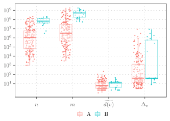
Figure 4: Basic properties of benchmark sets A and B: number of nodes $n$, number of edges $m$, median degree $\widetilde{d(v)}$ and maximum degree $\Delta_{v}$.

We evaluate our algorithm on a benchmark set composed of 197 graphs (referred to as set A), including 129 graphs from the 10th DIMACS Implementation Challenge [7], 25 randomly generated graphs [19, 29], 25 large social networks [30, 35], and 18 graphs from various application domains [14, 52, 50]. Scalability and experiments with larger values of $k$ are performed on a subset of set A that contains 21 graphs (referred to as set B). This benchmark set includes the 18 largest graphs (by number of nodes) and 3 randomly chosen small graphs of set A such that a partition with $2^{20}$ blocks only contains a few nodes per block. Basic properties of benchmark instances are shown in Appendix C, Figure 4.

Methodology.

We consider a combination of a graph and number of blocks $k$ as an instance. For each instance, we usually perform several runs with different random seeds and aggregate running times and edge cuts using the arithmetic mean over all seeds. To further aggregate over multiple instances, we use the harmonic mean for relative speedups, and the geometric mean for absolute running times and edge cuts. Runs with imbalanced partitions are not excluded from aggregated running times and for instances that exceeded the time limit, we use the time limit in the aggregates. We consider an instance as infeasible, if all runs failed or computed an imbalanced partition and mark them with ✗ in the plots.

To compare the solution quality of different algorithms, we use performance profiles [16]. Let $\mathcal{A}$ be the set of all algorithms we want to compare, $\mathcal{I}$ the set of instances, and $q_{A}(I)$ the quality of algorithm $A\in\mathcal{A}$ on instance $I\in\mathcal{I}$. For each algorithm $A$, we plot the fraction of instances $\frac{|\mathcal{I}_{A}(\tau)|}{|\mathcal{I}|}$ ($y$-axis) where $\mathcal{I}_{A}(\tau)\coloneqq\{I\in\mathcal{I}\leavevmode\nobreak\ |\leavevmode\nobreak\ q_{A}(I)\leq\tau\cdot\min_{A^{\prime}\in\mathcal{A}}q_{A^{\prime}}(I)\}$ and $\tau$ is on the $x$-axis. Achieving higher fractions at lower $\tau$-values is considered better. For $\tau=1$, the $y$-value indicates the percentage of instances for which an algorithm performs best. Since performance profiles relate the quality of an algorithm to the best solution, the ranking induced by $\tau=1$ does not permit full ranking of all algorithms, if more than two algorithms are included.

Running Time and Solution Quality for Small $k$.

In Figure 2 and Table 2 in Appendix D, we compare the quality and running time of KaMinPar with different partitioners for $k\in\{2,4,8,16,32,64\}$, $\varepsilon=0.03$ and $5$ repetitions per instance on set A and machine B. These are commonly used values to evaluate graph partitioning systems. Further, we execute each parallel partitioner using $10$ threads to simulate the performance of them on commodity machines.

KaMinPar 10 is the fastest algorithm on average and also an order of magnitude faster than the sequential partitioners Metis and KaHIP-fsocial on large graphs ($m\geq 10^{8}$), while producing partitions with comparable solution quality (see Figure 5 (left) in Appendix D). KaMinPar 10 (0,39 s geometric mean running time) is moderately faster than Mt-Metis 10 (0,48 s) and more than a factor of 2 resp. 3 faster than PuLP 10 (1,11 s) and Mt-KaHIP 10 (1,33 s). The differences in running time, as shown in Figure 2 (right), are more pronounced on larger instances, e.g., KaMinPar 10 (9,36 s) is more than factor of 3 resp. 5 faster than Mt-Metis 10 (30,36 s) resp. Mt-KaHIP 10 (55,76 s) on instances with more than $10^{8}$ edges. Figure 2 (left) shows that Mt-KaHIP 10 computes on most of the instances the partition with lowest edge cut ($\approx$ 60% of the instances), while the partitions produced by PuLP 10 are more than a factor of 2 worse than the best achieved edge cuts on more than 55% of the instances. These results are expected, since Mt-KaHIP is the only partitioner that implements a parallel direct $k$-way FM algorithm and PuLP is the only non-multilevel system in our evaluation. We perform the same experiment using $64$ cores of machine A on the larger instances of set B with similar results (see Appendix D). Thus, we can conclude that KaMinPar offers a compelling trade-off between running time and quality compared to established shared-memory and sequential GP systems.

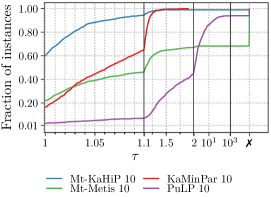
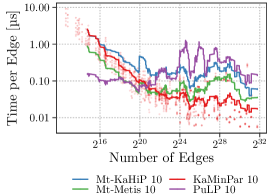
Figure 2: Performance profile and running time plot (shows time per edge with a right-aligned rolling geometric mean over 50 instances) comparing the performance of KaMinPar with different partitioners for smaller values of $k$ on set A.

Table 1: Results of our experiment for large values of $k$ with different parallel partitioners on set B. The last two columns show the geometric mean running time and edge cuts relative to KaMinPar of all instances that do not crash (timeout instances are additionally excluded in edge cut comparison).

Algorithm	# timeout	# crash	# imbalanced	# feasible	rel. time	rel. cut
KaMinPar 10	0	0	0	84	1,00	1,00
Mt-Metis-K 10	19	10	51	4	11,91	0,99
Mt-Metis-RB 10	0	25	55	4	5,61	1,03
Mt-KaHiP 10	31	7	11	35	38,64	1,00
PuLP 10	76	0	0	8	73,52	1,25

Running Time and Solution Quality for Large $k$.

In Table 1, we present the results of our experiment with different parallel partitioners (each using $10$ threads) for larger values of $k\in\{2^{11},2^{14},2^{17},2^{20}\}$, $\varepsilon=0.03$ and 3 repetitions per instance with a time limit of one hour on set B and machine B (192 Gb main memory). Note that the time limit is 10 times larger than the longest running time of KaMinPar for an instance. We additionally included the recursive bipartitioning version of Mt-Metis (referred to as Mt-Metis-RB) to evaluate the performance of recursive bipartitioning on large $k$. In the following, we consider a partition produced by an algorithm as feasible, if the algorithm terminates in the given time limit and satisfies the balance constraint $L_{k}\coloneqq(1+\varepsilon)\lceil\frac{c(V)}{k}\rceil$.

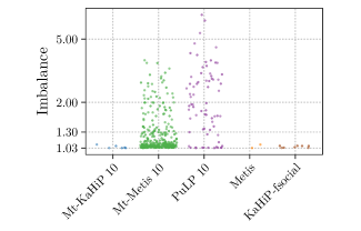
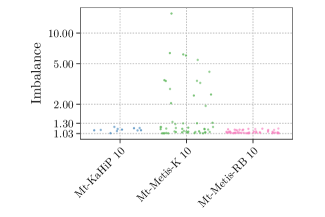
Figure 6: Left: imbalance of infeasible partitions computed by Mt-KaHiP 10, Mt-Metis 10, PuLP 10, Metis and KaHiP-fsocial on benchmark set A with $k\in\{2,4,8,16,32,64\}$ and $\varepsilon=0.03$. Right: imbalance of infeasible partitions computed by Mt-Metis-K 10, Mt-Metis-RB 10 and Mt-KaHiP 10 on benchmark set B with $k\in\{2^{11},2^{14},2^{17},2^{20}\}$ and $\varepsilon=0.03$.

Out of the 84 evaluated instances (21 graphs times 4 values of $k$), Mt-Metis-RB 10, Mt-Metis-K 10, PuLP 10 and Mt-KaHIP 10 were only able to produce on 4, 4, 8 resp. 35 instances a feasible solution. Mt-Metis-RB 10 and Mt-Metis-K 10 primarily failed to produce solutions that satisfy the balance constraint (55 resp. 51 instances). Figure 6 (right) in Appendix E shows that Mt-Metis-K 10 generally produces larger balance violations (median resp. maximum imbalance is 1,14 resp. 15,56) than Mt-Metis-RB 10 (median 1,05 and maximum 1,15). Mt-KaHIP 10 and PuLP 10 were mostly unable to compute a partition in the given time limit (31 resp. 76 instances). KaMinPar 10 produced a feasible solution on all instances. The fastest competitor is Mt-Metis-RB 10, which is more than 5 times slower than KaMinPar 10 on average. All other partitioners are an order of magnitude slower than KaMinPar 10. If we include all infeasible partitions and individually compare the partitioners on those instances in terms of solution quality, we can see that all produce partitions with comparable edge cuts (except for PuLP 10). However, a fair comparison in terms of solution quality is difficult due to the large number of infeasible solutions. We conclude that KaMinPar is currently the only partitioner considered in our evaluation that can reliably compute feasible partitions for larger values of $k$ in a reasonable amount of time.

Scalability of KaMinPar.

In Figure 3, we show the scalability of KaMinPar for $k\in\{2^{11},2^{14},2^{17},2^{20}\}$, $\varepsilon=0.03$ and three repetitions per instance on set B using $p\in\{1,4,16,64\}$ cores of machine A. In the plot, we represent the speedup of each instance as a point and the cumulative harmonic mean speedup over all instances with a single-threaded running time $\geq x$ seconds with a line. Note that initial partitioning includes all calls to our initial bipartitioning algorithms on graphs with more than $2pC$ nodes.

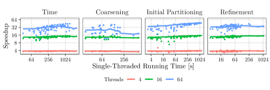
Figure 3: Self-relative speedups for the different components of KaMinPar on set B.

The overall harmonic mean speedup of KaMinPar is 3,8 for $p=4$, 13,3 for $p=16$ and 27,9 for $p=64$. The harmonic mean speedups of coarsening, initial partitioning and refinement are 25,0, 34,5 and 33,1 for $p=64$. We note that our refinement component achieves slightly better speedups than our coarsening component, although both are based on the size-constrained label propagation algorithm. This effect is most pronounced on instances with larger node degrees. During coarsening, each thread aggregates ratings to neighboring clusters in a local hash map (with only $2^{15}$ entries) for nodes with small degree and in a local vector of size $n$ for high degree nodes ($\geq 2^{15}/3$). During refinement, each thread uses a local vector of size $k$ for this. Instances with larger node degrees more often uses the local vector of size $n$ to aggregate ratings during coarsening, which can limit scalability due to cache effects. Note that KaMinPar performs no expensive arithmetic operations. Hence, perfect speedups are not possible due to limited memory bandwidth.

7 Conclusion and Future Work

We presented a new graph partitioning scheme that successfully combines the merits of classical direct $k$-way partitioning and recursive bipartitioning. Similar to direct $k$-way partitioning, deep MGP coarsens and uncoarsens the graph only once, and allows the use of $k$-way local improvement algorithms. Yet, it does not suffer scalability problems if $k$ is large and has a better asymptotic running time than recursive bipartitioning. Our experimental evaluation shows that our shared-memory parallel implementation of deep MGP runs efficiently on up to 64 PEs, while achieving comparable results to established graph partitioners if $k$ is small. Furthermore, our evaluation showed that KaMinPar is an order of magnitude faster than other graph partitioners based on direct $k$-way partitioning if $k$ is large, while consistently producing balanced solutions. In the future, we would like to explore graph partitioning for very large values of $k$, e.g., $k\in\Theta(n)$.

Appendix A Parallel Multilevel Graph Partitioning

Graph partitioners that are able to partition large real-world graphs can be categorized into three types of systems: streaming [48, 17, 49, 2, 36, 39], non-multilevel [46, 47] and parallel multilevel algorithms [45, 47, 13, 26, 5, 38]. Streaming graph partitioners operate in a model in which the nodes $v$ and their neighborhood arrive one at a time and the algorithm directly has to assign $v$ to a block. Non-multilevel systems such as PuLP [45, 47] directly partition the input graph into $k$ blocks and use local search heuristics to further improve solution quality. Streaming and non-multilevel systems significantly sacrifice solution quality to achieve higher speed [49, 36, 46, 17].

The matching [13, 15, 31, 26, 51] and clustering algorithms [5, 12, 22] used by different sequential partitioners in the coarsening phase are well-suited for parallelization, sometimes with only minor quality losses [12, 9]. The coarsening phase proceeds until a fixed number of nodes remains, usually $kC$, where $C$ is a tuning parameter.

In the initial partitioning phase, parallel partitioners either call sequential multilevel algorithms with different random seeds [5, 13, 15, 25] or use parallel recursive bipartitioning [22, 31, 26, 32]. In the former case, the graph is copied to each PE and the best partition obtained from all independent runs is projected back to the coarsest graph. In the latter case, parallelism is achieved by either splitting the thread pool into two evenly-sized groups and assigning each to one of the two recursive calls [26, 31] or dynamically assign the threads to the recursive calls with a task scheduler [22]. To obtain an initial bipartition of the coarsest graph, often portfolio approaches composed of different bipartitioning algorithms are used [41, 42, 22, 11].

Most parallel partitioners use the label propagation heuristic to improve the solution quality during the refinement phase [5, 31, 22, 38, 51, 15]. More advanced techniques are based on parallel variants of the FM local search [18] that are widely used in sequential partitioners. PT-Scotch [13], KaPPa [25] and Jostle [51] use sequential $2$-way FM refinement on two adjacent blocks of the partition. Mt-KaHIP [5] and Mt-KaHyPar [22] implement a parallel $k$-way FM algorithm based on the localized multi-try FM of the sequential graph partitioner KaHIP [41]. Mt-Metis [32] uses greedy refinement (FM with only positive gain moves), and hill-scanning, a simplification of localized FM where small groups of vertices, whose individual gains are negative, are moved if their combined gain is positive.

In the parallel setting, nodes can change their block concurrently which requires synchronization to ensure that the balance constraint is not violated [31]. Existing systems either explicitly communicate their local changes and reject moves that would violate the balance constraint [31, 26, 15] or use atomic compare-and-swap instructions to maintain block weights [22, 5].

Appendix B Proof of Theorem 4.1

Proof B.1.

By (3), MGP goes through $\log(n/C)$ levels so that the overhead terms “$\log n$” in (4) sum to $\mathcal{O}\!\left(\log^{2}n\right)$ – we ignore these overhead from now on. While $>pC$ nodes are left, the graph shrinks geometrically with the levels so that the total remaining cost for (un)coarsening and balancing from (4) is linear – $\mathcal{O}\!\left(n/p\right)$.

When $\leq pC$ nodes are left, replication and selection of the best partition keeps the number of nodes at each level at $\Theta\!\left(pC\right)$. There are $\log p$ such levels incurring total cost $\mathcal{O}\!\left(C\log p\right)$ for (un)coarsening and balancing. By (2) this cost is bounded by $\mathcal{O}\!\left(n/p\right)$.

For the cost of bipartitioning we consider three cases:
Case (a) $k\leq p$: Each PE performs $\log k$ bipartitions with total cost $C\log k$. By (2) this is bounded by $\mathcal{O}\!\left(n/p\right)$.
Case (b) $p<k\leq n/C$: Each PE performs $\log p+k/p$ bipartitions with total cost $C(k/p+\log p)$. Once more, by (2) this is bounded by $\mathcal{O}\!\left(n/p\right)$.
Case (c) $k>n/C$: In this case, deep MGP first performs an $n/C$-way partitioning into blocks of size about $C$. By the above analysis, this takes time $\mathcal{O}\!\left(n/p+\log^{2}n\right)$. Then the remaining blocks are partitioned into $k/(n/C)=kC/n$ blocks using recursive bipartitioning in time $\mathcal{O}\!\left(C\log(kC/n)\right)$. Summing over all blocks assigned to a PE we get additional cost $n\log(kC/n)/p$.

Appendix C Benchmark Set Statistics

Appendix D Running Time and Solution Quality with Small $k$

We also ran KaMinPar, Mt-Metis and Mt-KaHiP on all 64 cores of machine A. Here, we partitioned each graph of the reduced benchmark set B into $k\in\{2,4,8,16,32,64\}$ blocks allowing a maximum imbalance of $\varepsilon=0.03$. In this setup, KaMinPar 64 is 5 resp. 4,4 times faster than Mt-KaHiP 64 resp. Mt-Metis 64, whereas on the same instances on 10 cores of machine B, it is 5,7 resp. 3,1 times faster. Thus, we can see that the running time of KaMinPar scales slightly worse to 64 cores than Mt-KaHiP, but slightly better than Mt-Metis for smaller values of $k$. In Figure 5 (right), we compare the solution quality of each algorithm on the reduced benchmark set B. We can see that the differences of the partitioners in terms of solution quality are more pronounced on this set than on set A (compare with Figure 2). However, this is due to the benchmark set, since each partitioner produced partitions with comparable quality if we compare them individually with $10$ and $64$ threads.

Table 2: Geometric mean running time and solution quality for different algorithms on benchmark set A and $k\in\{2,4,8,16,32,64\}$. Running time only includes instances for which all algorithms produced a result. The number of included instances is shown in the last row. Solution quality is relative to KaMinPar (lower is better) and only includes instances for which the respective algorithm computed a balanced partition. Thus, solution quality cannot be compared between different competitors.

Algorithm	$T$	$T[m\geq 10^{6}]$	$T[m\geq 10^{8}]$	rel. cut	# infeasible
KaMinPar 10	0,39 s	0,85 s	9,36 s	1,00	0
Mt-Metis 10	0,48 s	1,49 s	30,36 s	1,00	349
Mt-KaHiP 10	1,33 s	3,84 s	55,76 s	0,94	6
PuLP 10	1,11 s	5,70 s	95,93 s	2,39	72
Metis	1,00 s	4,15 s	97,44 s	1,05	2
KaHiP-fsocial	2,93 s	11,05 s	200,67 s	1,03	8
# instances	1 150	832	196

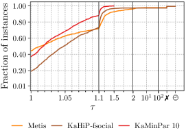
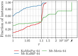
Figure 5: Left: performance profile of KaMinPar, Metis and KaHiP-fsocial on benchmark set A with $k\in\{2,4,8,16,32,64\}$ and $\varepsilon=0.03$. Right: performance profile of KaMinPar, Mt-KaHiP and Mt-Metis on 64 cores of machine A, reduced benchmark set B with $k\in\{2,4,8,16,32,64\}$ and $\varepsilon=0.03$. Note that the change in relative solution quality is due to the reduced benchmark set.

Appendix E Infeasible Solutions

References

- [1] Intel Threading Building Blocks. https://www.threadingbuildingblocks.org/.
- [2] Z. Abbas, V. Kalavri, P. Carbone, and V. Vlassov. Streaming Graph Partitioning: An Experimental Study. PVLDB, 11(11):1590–1603, 2018. doi:10.14778/3236187.3236208.
- [3] Y. Akhremtsev, T. Heuer, P. Sanders, and S. Schlag. Engineering a direct k-way Hypergraph Partitioning Algorithm. In 19th Workshop on Algorithm Engineering and Experiments, (ALENEX), pages 28–42, 2017.
- [4] Y. Akhremtsev. Parallel and External High Quality Graph Partitioning. PhD thesis, Karlsruher Institut für Technologie (KIT), 2019. doi:10.5445/IR/1000098895.
- [5] Y. Akhremtsev, P. Sanders, and C. Schulz. High-Quality Shared-Memory Graph Partitioning. IEEE Transactions on Parallel and Distributed Systems, 31(11):2710–2722, 2020. doi:10.1109/TPDS.2020.3001645.
- [6] K. Andreev and H. Räcke. Balanced Graph Partitioning. Theory of Computing Systems, 39(6):929–939, 2006.
- [7] D. Bader, H. Meyerhenke, P. Sanders, and D. Wagner, editors. 10th DIMACS Implementation Challenge – Graph Partitioning and Graph Clustering, 2012.
- [8] C. Bichot and P. Siarry, editors. Graph Partitioning. Wiley, 2011.
- [9] M. Birn, V. Osipov, P. Sanders, C. Schulz, and N. Sitchinava. Efficient Parallel and External Matching. In Euro-Par, volume 8097 of LNCS, pages 659–670. Springer, 2013.
- [10] A. Buluc, H. Meyerhenke, I. Safro, P. Sanders, and C. Schulz. Recent Advances in Graph Partitioning. In L. Kliemann and P. Sanders, editors, Algorithm Engineering, volume 9220 of LNCS, pages 117–158. Springer, 2014.
- [11] U. V. Catalyurek and C. Aykanat. Hypergraph-partitioning based Decomposition for Parallel Sparse-Matrix Vector Multiplication. IEEE Transactions on Parallel and Distributed Systems (TPDS), 10(7):673–693, 1999.
- [12] Ü. V. Çatalyürek, M. Deveci, K. Kaya, and B. Ucar. Multithreaded Clustering for Multi-Level Hypergraph Partitioning. In IEEE 26th International Symposium on Parallel and Distributed Processing (IPDPS), pages 848–859. IEEE, 2012.
- [13] C. Chevalier and F. Pellegrini. PT-Scotch. Parallel Computing, pages 318–331, 2008.
- [14] T. A. Davis and Y. Hu. The University of Florida Sparse Matrix Collection. ACM Transactions on Mathematical Software, 38(1):1:1–1:25, 2011.
- [15] K. D. Devine, E. G. Boman, R. T. Heaphy, R. H. Bisseling, and Ü. V. Catalyürek. Parallel Hypergraph Partitioning for Scientific Computing. In 20th International Conference on Parallel and Distributed Processing, (IPDPS), pages 124–124. IEEE, 2006.
- [16] E. D. Dolan and J. J. Moré. Benchmarking Optimization Software with Performance Profiles. Math. Program., 91(2):201–213, 2002. doi:10.1007/s101070100263.
- [17] M. F. Faraj and C. Schulz. Buffered Streaming Graph Partitioning. CoRR, abs/2102.09384, 2021. URL: https://arxiv.org/abs/2102.09384, arXiv:2102.09384.
- [18] C. M. Fiduccia and R. M. Mattheyses. A Linear-Time Heuristic for Improving Network Partitions. In Proceedings of the 19th Conference on Design Automation, pages 175–181, 1982.
- [19] D. Funke, S. Lamm, P. Sanders, C. Schulz, D. Strash, and M. von Looz. Communication-free Massively Distributed Graph Generation. In IEEE International Parallel and Distributed Processing Symposium (IPDPS), 2018.
- [20] M. R. Garey and D. S. Johnson. Computers and Intractability: A Guide to the Theory of NP-Completeness, volume 174. W.H. Freeman, San Francisco, 1979.
- [21] L. Gottesbüren, T. Heuer, P. Sanders, and S. Schlag. Shared-Memory n-level Hypergraph Partitioning. arXiv preprint arXiv:2104.08107, 2021.
- [22] L. Gottesbüren, T. Heuer, P. Sanders, and S. Schlag. Scalable Shared-Memory Hypergraph Partitioning. In 23rd Workshop on Algorithm Engineering and Experiments, (ALENEX 2021), pages 16–30. SIAM, 2021.
- [23] T. Heuer and S. Schlag. Improving Coarsening Schemes for Hypergraph Partitioning by Exploiting Community Structure. In 16th International Symposium on Experimental Algorithms, (SEA), pages 21:1–21:19, 2017.
- [24] T. Heuer, N. Maas, and S. Schlag. Multilevel Hypergraph Partitioning with Vertex Weights Revisited. arXiv preprint arXiv:2102.01378, 2021.
- [25] M. Holtgrewe, P. Sanders, and C. Schulz. Engineering a Scalable High Quality Graph Partitioner. 24th IEEE International Symposium on Parallel and Distributed Processing (IPDPS), pages 1–12, 2010.
- [26] G. Karypis and V. Kumar. Parallel Multilevel -way Partitioning Scheme for Irregular Graphs. In Proceedings of the ACM/IEEE Conference on Supercomputing, 1996.
- [27] G. Karypis and V. Kumar. A Fast and High Quality Multilevel Scheme for Partitioning Irregular Graphs. SIAM Journal on Scientific Computing, 20(1):359–392, 1998.
- [28] G. Karypis and V. Kumar. Multilevel k-way Partitioning Scheme for Irregular Graphs. Journal on Parallel and Distributed Compututing, 48(1):96–129, 1998.
- [29] F. Khorasani, R. Gupta, and L. N. Bhuyan. Scalable SIMD-Efficient Graph Processing on GPUs. In Proceedings of the 24th International Conference on Parallel Architectures and Compilation Techniques, PACT ’15, pages 39–50, 2015.
- [30] U. o. M. Laboratory of Web Algorithms. Datasets. URL: http://law.di.unimi.it/datasets.php.
- [31] D. LaSalle and G. Karypis. Multi-threaded Graph Partitioning. In 27th IEEE International Parallel and Distributed Processing Symposium (IPDPS), pages 225–236, 2013.
- [32] D. LaSalle and G. Karypis. A Parallel Hill-Climbing Refinement Algorithm for Graph Partitioning. In 45th International Conference on Parallel Processing (ICPP), pages 236–241, 2016.
- [33] D. Lasalle and G. Karypis. Multi-threaded Graph Partitioning. In 27th IEEE International Symposium on Parallel and Distributed Processing, IPDPS 2013, Cambridge, MA, USA, May 20-24, 2013, pages 225–236. IEEE Computer Society, 2013. doi:10.1109/IPDPS.2013.50.
- [34] D. LaSalle, M. M. A. Patwary, N. Satish, N. Sundaram, P. Dubey, and G. Karypis. Improving Graph Partitioning for Modern Graphs and Architectures. In Proceedings of the 5th Workshop on Irregular Applications - Architectures and Algorithms, IA3 2015, Austin, Texas, USA, November 15, 2015, pages 14:1–14:4. ACM, 2015. doi:10.1145/2833179.2833188.
- [35] J. Leskovec. Stanford Network Analysis Package (SNAP).
- [36] C. Martella, D. Logothetis, A. Loukas, and G. Siganos. Spinner: Scalable Graph Partitioning in the Cloud. In 33rd IEEE International Conference on Data Engineering (ICDE), pages 1083–1094, 2017.
- [37] H. Meyerhenke, P. Sanders, and C. Schulz. Partitioning Complex Networks via Size-Constrained Clustering. In Experimental Algorithms, volume 8504 of LNCS, pages 351–363. Springer, 2014. doi:10.1007/978-3-319-07959-2_30.
- [38] H. Meyerhenke, P. Sanders, and C. Schulz. Parallel Graph Partitioning for Complex Networks. IEEE Transactions on Parallel and Distributed Systems, 28(9):2625–2638, 2017. doi:10.1109/TPDS.2017.2671868.
- [39] J. Nishimura and J. Ugander. Restreaming Graph Partitioning: Simple Versatile Algorithms for Advanced Balancing. In 19th ACM SIGKDD Conf. on Knowledge Discovery and Data Mining (KDD), pages 1106–1114, 2013.
- [40] U. N. Raghavan, R. Albert, and S. Kumara. Near Linear Time Algorithm to Detect Community Structures in Large-Scale Networks. Physical review E, 76(3):036106, 2007.
- [41] P. Sanders and C. Schulz. Engineering Multilevel Graph Partitioning Algorithms. In 19th European Symposium on Algorithms (ESA), volume 6942 of LNCS, pages 469–480. Springer, 2011.
- [42] S. Schlag, V. Henne, T. Heuer, H. Meyerhenke, P. Sanders, and C. Schulz. -way Hypergraph Partitioning via -Level Recursive Bisection. In 18th Workshop on Algorithm Engineering and Experiments (ALENEX), pages 53–67, 2016.
- [43] K. Schloegel, G. Karypis, and V. Kumar. Graph Partitioning for High Performance Scientific Simulations. In The Sourcebook of Parallel Computing, pages 491–541, 2003.
- [44] C. Schulz and D. Strash. Graph Partitioning: Formulations and Applications to Big Data. In S. Sakr and A. Y. Zomaya, editors, Encyclopedia of Big Data Technologies. Springer, 2019. doi:10.1007/978-3-319-63962-8\_312-2.
- [45] G. M. Slota, K. Madduri, and S. Rajamanickam. PuLP: Scalable Multi-Objective Multi-Constraint Partitioning for Small-World Networks. In 2014 IEEE International Conference on Big Data (Big Data), pages 481–490, 2014. doi:10.1109/BigData.2014.7004265.
- [46] G. M. Slota, K. Madduri, and S. Rajamanickam. Complex Network Partitioning Using Label Propagation. SIAM J. Scientific Computing, 38(5), 2016. doi:10.1137/15M1026183.
- [47] G. M. Slota, S. Rajamanickam, K. D. Devine, and K. Madduri. Partitioning Trillion-Edge Graphs in Minutes. In 31st IEEE International Symposium on Parallel and Distributed Processing (IPDPS), pages 646–655, 2017.
- [48] I. Stanton and G. Kliot. Streaming Graph Partitioning for Large Distributed Graphs. In 18th ACM SIGKDD Conf. on Knowledge Discovery and Data Mining, (KDD), pages 1222–1230, 2012.
- [49] C. E. Tsourakakis, C. Gkantsidis, B. Radunovic, and M. Vojnovic. FENNEL: Streaming Graph Partitioning for Massive Scale Graphs. In 7th ACM Conference on Web Search and Data Mining, (WSDM), pages 333–342, 2014.
- [50] N. Viswanathan, C. Alpert, C. Sze, Z. Li, and Y. Wei. The DAC 2012 Routability-driven Placement Contest and Benchmark Suite. In 49th Design Automation Conference, (DAC), pages 774–782, 2012.
- [51] C. Walshaw and M. Cross. JOSTLE: Parallel Multilevel Graph-Partitioning Software – An Overview. In Mesh Partitioning Techniques and Domain Decomposition Techniques, pages 27–58. 2007.
- [52] S. Williams, L. Oliker, R. Vuduc, J. Shalf, K. Yelick, and J. Demmel. Optimization of Sparse Matrix-Vector Multiplication on Emerging Multicore Platforms. In SC ’07: Proceedings of the 2007 ACM/IEEE Conference on Supercomputing, pages 1–12, 2007. doi:10.1145/1362622.1362674.