Instance segmentation of fallen trees in aerial color infrared imagery using active multi-contour evolution with fully convolutional network-based intensity priors

Abstract

Over the last several years, semantic image segmentation based on deep neural networks has been greatly advanced. On the other hand, single-instance segmentation still remains a challenging problem. In this paper, we introduce a framework for segmenting instances of a common object class by multiple active contour evolution over semantic segmentation maps of images obtained through fully convolutional networks. The contour evolution is cast as an energy minimization problem, where the aggregate energy functional incorporates a data fit term, an explicit shape model, and accounts for object overlap. Efficient solution neighborhood operators are proposed, enabling optimization through metaheuristics such as simulated annealing. We instantiate the proposed framework in the context of segmenting individual fallen stems from high-resolution aerial multispectral imagery, providing problem-specific energy potentials. We validated our approach on 3 real-world scenes of varying complexity, using 730 manually labeled polygon outlines as ground truth. The test plots were situated in regions of the Bavarian Forest National Park, Germany, which sustained a heavy bark beetle infestation. Evaluations were performed on both the polygon and line segment level, showing that the multi-contour segmentation can achieve up to 0.93 precision and 0.82 recall. An improvement of up to 7 percentage points (pp) in recall and 6 in precision compared to an iterative sample consensus line segment detection baseline was achieved. Despite the simplicity of the applied shape parametrization, an explicit shape model incorporated into the energy function improved the results by up to 4 pp of recall. Finally, we show the importance of using a high-quality semantic segmentation method (e.g. U-net) as the basis for individual stem detection, as the quality of the results degraded dramatically in our baseline experiment utilizing a simpler method. Our method is a step towards increased accessibility of automatic fallen tree mapping in forests, due to higher cost efficiency of aerial imagery acquisition compared to laser scanning. The precise fallen tree maps could be further used as a basis for plant and animal habitat modeling, studies on carbon sequestration as well as soil quality in forest ecosystems.

1 Introduction

Forest ecosystems are the most species-rich ecosystems on earth and play an essential role in providing ecosystem services such as wood production, drinking water supply, carbon sequestration, and biodiversity preservation (Watson et al., 2018). However, forests are under immense pressure especially because of the unsustainable use of their resources, conversion into other land use types, and global change. Therefore, there is a strong need for better management and conservation practises allowing a sustainable use that can secure all the services. A critical precondition for sustainable forest management are monitoring schemes that provide the necessary information for preparing management plans. Besides growing stock, yield and tree species distribution, also deadwood is an essential indicator of forest health as e.g. in temperate forests, up to one-third of all species depend on it during their life cycle (Müller and Bütler, 2010). Moreover, it is not just the amount of deadwood that matters for the conservation of biodiversity (Seibold and Thorn, 2018); also its quality is decisive for the conservation of biodiversity. Therefore, it is also important to determine the tree species, the decay stage and if the dead wood is standing or lying. Estimating the amount of both types of deadwood is not just decisive for the maintaining biodiversity, but also for management of adverse effects of forest disturbances such as wind throws and insect outbreaks. The latter aspect is becoming increasingly important as the frequency and severity of such disturbance events are continuously on the rise due to global change (Seidl et al., 2017). Such events can affect large tracks of forested land in a short time span (e.g. windthrow). That makes it very difficult to accurately assess the amount of timber affected by conventional field-based methods. Therefore, remote sensing techniques are a natural and cost-efficient alternative to field works. This demand for accurate information on the distribution of coarse woody debris (CWD) in forests, driven by the aforementioned factors, has sparked research interest within the remote sensing community. In recent years, a number of contributions have focused on detection and classification of dead wood from laser scanning data (Marchi et al., 2018). Delineating individual fallen stems in both aerial (e.g. Polewski et al. (2015a)) and terrestrial (e.g. Polewski et al. (2017)) point clouds was shown to be feasible.

While the 3D information inherent in laser scanning point clouds provides a solid basis for fallen tree detection, obtaining high density laser scanning data may be prohibitively expensive. Multispectral aerial imagery offers a more accessible alternative. The near-infrared channel is particularly useful for this purpose, since dead and diseased vegetation produces a distinct reflectance signature in this spectral band (Jensen, 2006). In case of fallen tree stems, resolution at the level of decimeters or better is crucial to the success of detection, because the width of the target object can be as low as 30-40 cm, and as such they could appear as only a single row of pixels (or be altogether missing) within a lower-resolution image. A number of studies considered the determination of tree health (e.g. Safonova et al. (2019)) or direct detection of coarse woody debris (e.g. Freeman et al. (2016)) from high-resolution optical imagery. Currently, most approaches dealing with fallen trees focus on either analyzing groupings of pixels without a one-to-one correspondence to stems (e.g. Einzmann et al. (2017); Lopes Queiroz et al. (2019)), or determining lines which represent the positions and lengths of individual trees, disregarding their thickness (Panagiotidis et al., 2019; Duan et al., 2017).

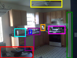
(a)

(b)

(c)

Figure 1: (a)-(b) sample images from the LSVRC dataset (Russakovsky et al., 2015). The data is geared towards high-resolution close-range photography from handheld devices. (c) sample nadir-view color infrared image showing multiple intersecting fallen stems.

This paper considers the task of delineating single fallen stems in the broader context of instance segmentation in imagery. Our goal is to extract polygons representing individual stems from difficult scenarios which contain dozens of partially overlapping and intersecting objects (see Fig. 1). While dense semantic segmentation of images has been arguably all but solved using decoder-encoder architectures like fully convolutional networks (e.g. Ronneberger et al. (2015)), extraction of individual object instances still remains a challenge and an active area of research within the neural network and computer vision community (Arnab and Torr, 2017; He et al., 2017). State-of-the-art approaches based on convolutional neural networks(CNN) suffer from coarseness of feature maps and limited information contained in the candidate object regions of interest, which leads to degraded performance for small and multi-scale object localization (Zhao et al., 2018). Also, some of the recent advancements have been geared towards benchmarks and competitions published by the computer vision community, such as the Large Scale Visual Recognition Challenge (LSVRC) (Russakovsky et al., 2015). These datasets usually contain large quantities of close-range images captured from handheld devices, depicting clearly-visible ’common’ objects such as household items, people, animals, etc. The emphasis is put on the network’s ability to recognize a variety of object classes (the LSVRC data contains 200 categories). In contrast, remote sensing images, especially acquired in a natural resource monitoring setting, usually contain many possibly overlapping instances of the same object category, like fallen trees in a bark beetle attack zone (Fig. 1) or a cluster of tree crowns. Although the optical sensor hardware is improving, the average resolution of aerial remote sensing imagery is still significantly smaller than in case of close-range photography, resulting in possibly blurred object boundaries. This could pose a problem to some of the state-of-the-art CNN architectures which follow a region proposal-classification design (e.g. Ren et al. (2017)). Overlapping region proposals, containing candidate object bounding boxes, are usually pruned using a discrete process like non-maxima suppression, which means that if the candidate generator produces a high ’objectness’ score on an image region not centered on a real object (due to blurred boundaries and heavy candidate overlap), the true detections could be thrown away and never even make it to the classification stage. Moreover, specifically for the case of fallen stems, detection based on axis aligned bounding boxes has a key weakness. Typically, imagery obtained in remote sensing flight campaigns features a ground sampling distance of no less than 10-15 cm. Therefore, fallen tree trunks would appear only several pixels wide and possibly hundreds of pixels long. Assuming that the stems may be arbitrarily oriented within the image, the tree’s axis-aligned bounding box would be overwhelmingly populated with irrelevant pixels (except close to the main diagonal).

To alleviate some of these problems, we introduce a general framework for segmenting sets of overlapping objects of a single category into individual instances. Instead of attempting to detect objects in axis-aligned bounding boxes, we maintain shape parametrizations and associated rigid transform parameters separately per instance, effectively evolving multiple active contours (Cremers et al., 2007) simultaneously. Our framework explicitly models object overlap as well as prior shape information. Starting from an initial random state and an upper bound on the number of objects in the scene, the optimization process eliminates redundant shapes by evolving them to empty contours. The method operates on the probability maps produced by dense semantic segmentation, taking advantage of object appearance prior information learned from training examples. We instantiate the framework specifically for fallen tree stem detection, evolving rectangular shapes according to the energy functional which combines a nonparametric shape prior, a data fit term, and a collinearity model. We propose a simulated annealing scheme with stochastic sampling as the method of choice for evolving the optimal shapes and their spatial orientations. The evaluated energy is defined on the space of polygons. The target polygons are obtained by finding contours of 0.5-superlevel sets of probability images from semantic segmentation. This enables efficient computation of energy changes from applying neighboring moves, because calculating intersections between the rectangular shapes and the target polygons can be carried out with log-linear time complexity with respect to the number of edges in the polygons (Žalik, 2000), as opposed to being a function of the number of image pixels.

The rest of this paper is organized as follows. In Section 2, we report related work regarding both the detection of fallen trees from imagery and methodological aspects of combining active contour methods with CNN based segmentation. Section 3 introduces the general framework for instance segmentation of images based on multi-contour evolution on an abstract level, whereas in Section 4, the framework is instantiated for detecting fallen trees; we provide details of the tailored solution neighborhood operator for the stochastic optimization, the initialization strategy as well as specific realizations of the shape prior and other elements of the energy functional. In Section 5, experimental evaluations of the proposed method are provided, in comparison to a baseline operating on line level. Also in this section we investigate the impact of using a CNN for generating the appearance prior versus a simple baseline derived from raw image channel intensities. The experimental results are discussed in Section 6, and the most important conclusions are summarized in the final section.

2 Related work

To the best of our knowledge, this is the first contribution addressing the large scale detection of fallen stems from aerial imagery on a polygon level, which provides a comprehensive evaluation on over 700 reference polygons. From an application standpoint, the two approaches conceptually most similar to ours use the Hough transform to fit lines representing individual stems in binarized images of target class posterior probabilities obtained on the basis of hand-crafted textural features (Duan et al., 2017) or spectral thresholding (Panagiotidis et al., 2019). Thiel et al. (2020) performed generic line detection within RGB orthomosaics derived from very-high resolution unmanned aerial system-acquired imagery to find approximate fallen stem shapes.Lopes Queiroz et al. (2019) used a generic segmentation procedure on the spectral bands of the aerial image combined with the normalized difference vegetation index (Tucker, 1979), and subsequently classified the resulting clusters based on spectral/textural features augmented with LiDAR derived information (canopy height model). Einzmann et al. (2017) applied a similar approach, using large-scale mean shift in the role of the segmentation algorithm and augmenting the set of spectral bands with linear transformations of raw bands, textural features and multiple vegetation indices. However, neither of these approaches restricts the generic image segmentation to follow the shape or appearance of fallen stems, therefore in case of multiple intersecting trees, individual stems would not be delineated. We believe that a key advantage of our proposed method versus generic segmentation approaches is that the former has knowledge of the target object’s shape, whereas the latter do not. Therefore, while it may be possible to find parameters of generic methods that produce acceptable segmentations for any particular scene, these parameters (e.g. bandwidths, number of clusters) and not readily learnable from training data or easily transferable between scenes. In contrast, our method is informed on the dimensions of fallen stems as well as on the interactions between them, allowing it to decompose the scene into objects which plausibly look like fallen stems. On the area level,  Latifi et al. (2018) used synthetic RapidEye images to assess the extent of damage in spruce stands resulting from a bark beetle infestation. Regarding the use of deep neural networks for detecting diseased and dead trees, Safonova et al. (2019) applied a CNN to classify tree vitality from patches of RGB aerial imagery. Ostovar et al. (2019) used the Faster R-CNN (Ren et al., 2017) to detect regions of close-range images containing tree stumps, which were then classified with respect to their root and butt-rot status.

On a more abstract level, our method could be interpreted as a way of integrating CNNs with (multiple) active contour segmentation. Other ways of achieving this were previously reported by several authors. In the context of individual building segmentation from aerial imagery, Marcos et al. (2018) proposed an end-to-end trainable framework utilizing CNNs for learning the geometric prior parametrizations of an active contour model (ACM). Inference from the ACM was integrated into the CNN weight update schedule through computing a structured loss on the predicted and ACM’s predicted output versus ground truth polygons, and backpropagating the loss to the CNN parameters.

Our proposed approach borrows some ideas from the work of Cremers and Rousson (2007), where the active contour energy functional was designed to interact with the input image indirectly through the intensity priors. The authors also directly modeled the prior distribution of the shape coefficients using a kernel density estimator. Our energy formulation shares some similarities with the energy function utilized by Milan et al. (2014) for multiple object tracking, which also included a data fit term, pairwise interaction terms between tracked objects as well as unary potentials encoding physical motion constraints (analogous to proir information).

3 Multi-contour segmentation with priors

We consider the generic problem of fitting multiple instances of a single object class from abstract ’images’. Although all objects are by construction of the same class, a reasonable amount of intra-class variation in shape as well as appearance is allowed and expected. Usually, the image space $\mathbb{I}$ will correspond to either the image plane $\mathbb{R}^{2}$ or 3D Euclidean space $\mathbb{R}^{3}$, allowing to model e.g. 2D rasters or (voxelized) 3D point clouds. However, any vector space is viable where there is a meaningful concept of shape, rigid transformations (isometries) and a way of measuring shape overlap. Denoting an input image as $I\in\mathbb{I}$ sampled from the image space, we assume that $I$ contains an unknown number $M$ of object instances from the target class $C$. Our goal is to retrieve approximations of the target objects with respect to a pre-specified shape model $P_{s}(\bar{\alpha})$ and its associated shape generator function $f_{s}(\bar{\alpha})$, parameterized by a vector of abstract shape coefficients $\bar{\alpha}$. The shape generator instantiates shapes in standard position (centroid at the coordinate system origin, no rotations around axes). This function may be as complex as a generative adversarial network, where the shape coefficients represent the randomly sampled noise input, or as simple as a rectangle generator parameterized by a width and a height. Additionally, each modeled shape is equipped with its own set of position/orientation parameters $\theta_{i}$ which would typically include translations with respect to each coordinate axis and appropriate rotations as required by the dimensionality of $\mathbb{I}$. We will denote the shape generated by $f_{s}$ for coefficients $\bar{\alpha}$ and rigidly transformed by $\theta$ as $f_{s}(\bar{\alpha}|\theta)$.

In order to decouple shape and appearance (i.e. image intensity) information, we introduce an explicit discriminative prior $P_{i}(C|I)$ on the image space $\mathbb{I}$. This image intensity prior transforms the original, possibly multi-channel $I$ into a new probability image $I_{p}$ encoding the class probabilities of $C$ given the intensities. In practice, this can be seen as the output of a semantic segmentation, like the U-net (Ronneberger et al., 2015) in case of 2D raster images, or VoxNet (Maturana and Scherer, 2015) for voxelized 3D point clouds. By extracting contours of $q-$level supersets of $I_{p}$ (using e.g. the marching cubes algorithm by Lorensen and Cline (1987)), we may obtain a partition of $I$ into regions corresponding to the target class, or ’foreground’, versus ’background’ regions. The comparison between shapes evolving according to the model $P_{s}$ and ’foreground’ shapes present within the image now boils down to the calculation of set intersections and differences. Indeed, the shape model does not interact with the original image $I$ other than through the extracted level supersets from $I_{p}$. We define the collection of connected regions inside the probability image $I_{p}$ as $S=\{s_{i}\subset I_{p},i=1\ldots n_{s}\}$, corresponding to the extracted level supersets. The elements of $S$ form polytopes of appropriate dimension, e.g. polygons in 2D and polyhedrons in 3D. Note that these polytopes need not represent single instances of the target objects. In highly complicated scenarios, we expect them to consist of many intersecting and overlapping instances.

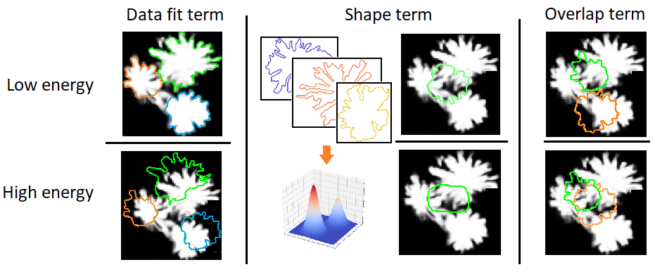
Figure 2: Illustration of the impact of the various terms on the aggregate energy function, which is a linear combination of the data fit, shape, and overlap potentials. Left column: data fit potential ensures that a large percentage of high-probability target class areas are covered by the evolving contours. Middle column: shape potential ensures that the evolved shapes are within the expected variability of the target objects’ shape distribution. Right column: overlap term prevents covering the same parts of the image with different evolving contours.

3.1 Energy function

Based on the definitions from the previous section, we are now ready to introduce the energy function which drives the evolution of the modeled shapes. Let $M^{\prime}$ denote an initial overestimation of the true number of objects $M$ inside the input image. Then, each evolving shape is described by its vector of shape coefficients $\bar{\alpha}_{i}$ as well as the location/orientation parameters $\theta_{i}$. Collecting all models parameters into a vector $\Omega=(\omega_{i}=(\bar{\alpha}_{i},\theta_{i}))_{i=1\ldots M^{\prime}}$, let $F(\omega_{i})$ be an alias for $f_{s}(\alpha_{i}|\theta_{i})$. The aggregate energy of the shape set is given by Eq. 1:

$$\begin{split}E(\Theta|S)=&\underbrace{\gamma_{d}E_{d}\left[\bigcup_{s\in S}s,\bigcup_{i}F(\omega_{i})\right]}_{\text{data fit term}}-\underbrace{\gamma_{s}\sum_{i}\log P_{s}(\bar{\alpha_{i}})}_{\text{shape probability term}}\\ &+\underbrace{\gamma_{o}\sum_{j,k,j\neq k}E_{o}[F(\omega_{j}),F(\omega_{k})]}_{\text{pairwise overlap term}}\\ &+\underbrace{\sum_{u}\tau_{u}E_{aux,u}(\Omega)}_{\text{auxiliary potentials}}\end{split}$$ (1)

An illustration of each energy term/potential’s role and impact on the aggregate energy is given by Fig. 2.

3.1.1 Data fit potential

The role of the data fit term $E_{d}(\tau,\phi)$ is to ensure that the model shapes coincide well with the target class regions of the image. It is a function of two sets: (i) the union $\tau$ of all target class regions $s\in S$ extracted from the probability image $I_{p}$, and (ii) the union $\phi$ of all currently modeled shapes obtained from ’decoding’ the elements of $\Omega$ with the generator function $f_{s}$ and applying the respective rigid transform. Ideally, the sets (i) and (ii) should coincide, however in practice the differences $\tau\setminus\phi$ as well as $\phi\setminus\tau$ are non-empty. The former corresponds the parts of regions designated as ’target class’ that are not covered by any model shape (false negatives). Symmetrically, $\phi\setminus\tau$ indicates regions deemed as ’target class’ by the model, but not intersecting with any elements $s\in S$, and thus lacking evidence in the input image (false positives). The value of $\tau\setminus\phi$ impacts the specificity/recall of the segmentation, whereas $\phi\setminus\tau$ impacts the sensitivity/precision. We allow an assignment of different weights to these two quantities, reflecting the fact that the tradeoff between precision and recall may be asymmetric for some applications:

$$E_{d}(\tau,\phi)=2[(1-\pi_{p})\lambda(\tau\setminus\phi)+\pi_{p}\lambda(\phi\setminus\tau)]$$ (2)

In the above, the term $\lambda(\cdot)$ can be thought of as analogous to the Lebesgue measure on the Euclidean space of the appropriate dimension, i.e. area in 2D, volume in 3D, etc. The term related to the precision (false positives) is weighted with $0\leq\pi_{p}\leq 1$.

3.1.2 Shape probability potential

This term is directly derived from the prior shape model $P_{s}(\bar{\alpha})$ as the sum of negative log-likelihoods of all model shapes. It acts as a regularizer for the shape coefficients, penalizing shapes which become too unlikely with respect to the learned prior. Note that for some generator functions, the shape coefficients $\bar{\alpha}$ may already be distributed uniformly by construction inside the (appropriately scaled) unit hypercube, in which case the shape probability term boils down to a constant and may be removed. For an example, see e.g.(Polewski et al., 2020), where a generative adversarial network with uniformly distributed latent variables was used as the shape model within the active contour segmentation framework.

3.1.3 Overlap potential

Since our framework assumes that initial guess on the number of shapes $M^{\prime}$ is biased towards too high values, we expect that part of the model shapes will become redundant. To prevent duplicate coverage of the same image regions by different model objects, and to allow the number of active shapes to converge to the true number of objects present within the image, we define an overlap potential $E_{o}$ which penalizes overlapping of model shapes. Acting together with the data fit term $E_{d}$, it is designed to direct a redundant shape towards evolving into an empty contour: $E_{o}$ will push a shape away from areas already occupied by other model shapes, while $E_{d}$ will ensure that the shape does not occupy background regions of the input image. Note that not all forms of overlap should be penalized. For example, in our application of fallen tree segmentation, intersections of tree stems that are not parallel to each other are unlikely to be due to instance duplication, instead they are the result of physical overlap and stacking. To model this, we utilize an auxiliary term $\kappa(o_{1},o_{2})\in[0;1]$ which quantifies the likelihood of model shapes $o_{1},o_{2}$ belonging to the same real-world object. The overlap potential is then defined in a pairwise manner as:

$$E_{o}(o_{1},o_{2})=\kappa(o_{1},o_{2})\lambda(o_{1}\cap o_{2})$$ (3)

The potential $E_{o}$ is evaluated over all pairs $i,j\in{1,2,\ldots,M^{\prime}}$ such that $i<j$, with each value contributing to the total energy $E(\Theta)$ in equal proportion. Once again, $\lambda$ indicates the ’natural’ measure in the Euclidean space of the appropriate dimension (area, volume etc.).

3.1.4 Auxiliary potentials

Our framework allows for application specific potentials $E_{aux,u}$, each weighted by their own coefficient $\tau_{u}$. In our formulation, to maintain the highest flexibility, these potentials are functions of the entire model parameter vector $\Omega$, which means they have access to both the shape coefficients and the decoded/transformed model shapes. This formulation admits unary, pairwise, or even higher order potentials. In Section 4, an example of an auxiliary pairwise potential is shown, which is designed to discourage collinearity between the modeled stems.

3.2 Relationship to active contour segmentation

The proposed framework can be viewed as one possible generalization of the classic foreground-background active contour raster image segmentation (Cremers et al., 2007) to multiple object instances and more general images. The statistical formulation by Cremers and Rousson (2007) assumed that the evolving contour of a target class $C$ region has an abstract shape parametrization $\bar{\alpha}$, endowed with a prior model $P_{s}(\bar{\alpha})$. The optimized energy functional represented a trade-off between the data fit term and probability of the evolving shape. Denoting $H_{\bar{\alpha}}[x]$ as the indicator function for image element $x$ lying inside the shape, their energy objective can be written as:

$$\begin{split}E^{\prime}(\bar{\alpha})=&-\int(H_{\bar{\alpha}}[x]\log P(x|C)\\ &+(1-H_{\bar{\alpha}}[x])\log P(x|\neg C))dx\\ &-\log P_{s}(\bar{\alpha})\end{split}$$ (4)

Here, the foreground and background regions have their separate image intensity likelihoods $P(x|C),P(x|\neg C)$. By assuming equal prior probabilities on the foreground/background regions ($P(C)=P(\neg C)$), based on the Bayesian rule we can express the data fit potential in terms of the target class posterior $P(C|x)$, resulting in:

$$\begin{split}E^{\prime\prime}(\bar{\alpha})&=-\underbrace{\int H_{\bar{\alpha}}[x]\log P(C|x)dx}_{\text{data fit inside contour}}\\ &-\underbrace{\int(1-H_{\bar{\alpha}}[x])\log[1-P(C|x)])dx}_{\text{data fit outside contour}}\\ &-\log P_{s}(\bar{\alpha})\\ &=E^{\prime}(\bar{\alpha})+D\end{split}$$ (5)

The new energy function $E^{\prime\prime}$ differs from $E^{\prime}$ only by a constant value $D$, therefore their extrema coincide (see e.g. Polewski et al. (2015b)). Moreover, under certain assumptions, the data fit terms inside and outside of the contour are analogous to the quantities $\lambda(\tau\setminus\phi)$ and $\lambda(\phi\setminus\tau)$ from our data fit potential (Eq.2). Specifically, recall that the target connected regions $s_{i}\in S$ are high-probability $q-$level supersets extracted from the probability image. We can therefore view the posterior class probability inside and outside these regions as respectively $p_{in}\approx 1-\epsilon,p_{out}\approx\epsilon$, where $\epsilon$ is a small positive constant. In this setting, the intersection of all objects modeled by the current state $\Omega$ with the set of target regions $S$ will contribute $\lambda(\tau\cap\phi)\cdot\log(1-\epsilon)\approx 0$ to the data fit potential, since $\log(1-\epsilon)$ tends to 0 with $\epsilon$. On the other hand, the difference $\phi\setminus\tau$ will contribute $\lambda(\phi\setminus\tau)\cdot\log\epsilon$, which tends to $-\infty$ as $\epsilon$ tends to zero. By a similar argument, one can show that the data fit term outside the contour from Eq. 5 is dominated by the symmetrical expression $\lambda(\tau\setminus\phi)\cdot\log\epsilon$. Setting $\pi_{p}$ to 0.5 in our data fit potential (Eq. 2), we see that an instantiation of our framework with a single modeled object is equivalent to the original statistical active contour formulation with probabilities quantized at ${1-\epsilon,\epsilon}$ such that $\gamma_{d}=-\log\epsilon$.

3.3 Optimization

To optimize the total energy from Eq. 1, various stochastic and combinatorial techniques are available based on the choice of quantization or lack thereof for the model variables. If all shape and rigid transformation parameters are continuous, Eq. 1 can be minimized using stochastic methods like simulated annealing (Kirkpatrick et al., 1983) or a hybrid Monte Carlo-gradient based approach like basin hopping (Wales and Doye, 1997; Li and Scheraga, 1987). The latter is particularly useful in settings where the gradients of all the energy function terms with respect to all model variables may be computed analytically. Sometimes it may be reasonable to discretize the domain of one or more variables, e.g. the shape translation parameters from $\theta_{i}$ could be expressed in pixels or voxels. In such cases, generic metaheuristics for solving mixed combinatorial/continuous problems are applicable, including methods from the class of evolutionary algorithms, specialized versions of tabu search (e.g. (Siarry and Berthiau, 1997)), and simulated annealing.

The aforementioned metaheuristics are based on exploring the neighborhood of the current solution and making local moves which alter a small part of it. This makes it cumbersome and inefficient to apply these local-search based methods to the minimization of our energy (Eq. 1), since the data fit term requires a union of all of the evolving shapes $\phi=\bigcup_{i}F(\omega_{i})$, and an intersection of this union with the high-probability object contours from the input image $\tau=\bigcup_{s\in S}s$. Even if only one shape $\omega_{i}$ is altered, all of the aforementioned calculations need to be repeated to re-evaluate the data fit potential $E_{d}$. To localize the effects of modifying individual shapes and make local search steps more efficient, we propose the following approximation. First, observe that as $\tau$ does not depend on the model variables, it can be precomputed once and reused in the calculations. Moreover, we may express the intersection $\phi\cap\tau$ as a union of intersections $\bigcup_{i}\tau\cap F(\omega_{i})$. Applying the inclusion-exclusion principle, we can write:

$$\begin{split}|\phi\cap\tau|&=\underbrace{\sum_{i}|\tau\cap F(\omega_{i})|}_{\text{unary term}}-\underbrace{\sum_{i\leq i<j}|\tau\cap F(\omega_{i})\cap F(\omega_{j})|}_{\text{pairwise term}}\\ &+\underbrace{\sum_{k=3}^{M^{\prime}}(-1)^{k+1}(\sum_{1\leq i_{1}<\ldots<i_{k}}|\tau\cap F(\omega_{i_{1}})\cap\ldots\cap F(\omega_{i_{k}})|)}_{\text{residual}}\end{split}$$ (6)

We choose to approximate $|\phi\cap\tau|$ by its underestimation given by the first two terms (unary and pairwise) in the inclusion-exclusion expansion (Eq. 6). This corresponds to ignoring contributions from subsets where 3 or more of the model shapes intersect. In practice, we believe this approximation is sufficient, because the model explicitly discourages overlap of multiple shapes through the overlap potential $E_{o}$. Moreover, by using an underestimation of the true intersection area $|\phi\cap\tau|$, the multi-shape overlap is penalized even more due to the subtraction of the overlapping area in the pairwise term and not recovering it in the (removed) residual. This leads the model away from undesirable overlap. However, the main benefit is that the influence of changing a single model shape $i$ (by mutating its shape coefficients or rigid transform parameters) is now reduced to affecting one unary term $|\tau\cap F(\omega_{i})|$ and at most $M^{\prime}$ pairwise terms $|\tau\cap F(\omega_{i})\cap F(\omega_{j})|,j\in{1,\ldots,M^{\prime}}$. The pairs $i,j$ which do not intersect can be filtered out using simple bounding box criteria. Combined with caching the values $|\tau\cap F(\omega_{i})|,|\tau\cap F(\omega_{i})\cap F(\omega_{j})|$ for all model objects and their pairs, the term $|\tau\setminus\phi|$ can be efficiently updated based on the values of $|\tau\cap\phi|,|\tau|$, by using the identity $|A\setminus B|=|A|-|A\cap B|$. In a similar manner, the value of $\phi$ may be approximated by caching and updating the first and second-order terms of the inclusion-exclusion expansion $|F(\omega_{i})|,|F(\omega_{i})\cap F(\omega_{j})|$, yielding $|\phi\setminus\tau|$. Moreover, the caching of the pairwise terms $|F(\omega_{i})\cap F(\omega_{j})|$ also enables fast updates of the term $E_{o}$. Finally, the shape model $P_{s}$ is already in additive form, therefore altering $\bar{\alpha_{i}}$ influences only the $\log P_{s}(\bar{\alpha_{i}})$. Care should be taken when instantiating auxiliary potentials to ensure that they also allow efficient partial updates, leading to applicability of local solution perturbation based metaheuristics.

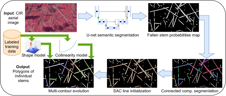
Figure 3: Overview of the processing pipeline for delineating individual stem polygons using multiple active contour evolution. The input CIR image undergoes semantic segmentation using the U-net, and the fallen stem probability map is partitioned into high-probability connected components. Next, the model shape positions and dimensions are initialized based on sample consensus line segmentation. Finally, the model shape configuration is optimized using simulated annealing, under consideration of the shape and collinearity models learned from labeled training data.

4 Application of our framework to the instance segmentation of fallen trees

In this section, we instantiate the framework described in the previous chapter, obtaining a method for detecting individual fallen stems from aerial imagery. We consider a 2D raster image with $N_{c}$ channels as input. Ideally, the image should include a near-infrared channel, which is known to differentiate dead and living vegetation well. The rest of this section explains the instantiation of various components of the energy term, the strategy for exploring the solution space using the neighborhood operator, as well as an initialization scheme based on detecting lines using the sample consensus method. An overview of the entire processing pipeline is depicted in Fig. 3.

4.1 Fully convolutional networks

Fully convolutional networks (FCNs) are a class of convolutional artificial neural networks (CNNs) designed for dense semantic segmentation of raster images. As opposed to classical CNNs that are used primarily for image (sparse) classification (i.e. assigning a single label to an entire image or patch), FCNs do not possess fully connected layers, which makes them independent of the input image size (Long et al., 2015). FCNs primarily consist of convolutional/transposed convolutional filters as well as pooling layers, organized into two symmetrical paths. The encoder path downsamples the original image into meaningful features by means of convolutional filters and pooling operations, whereas the upsampling path aims at decoding these features into a full-sized output map using transposed convolution operations. The final, topmost upsampling layer of the network is fed into a softmax operator, producing per-class posterior probabilities at each pixel and enabling end-to-end training with a logistic loss function. A classic FCN architecture which attained widespread use across various applications (Akeret et al., 2017; Dong et al., 2017) is the U-net (Ronneberger et al., 2015), where upsampling layers are augmented with feature maps from the downsampling path at the corresponding resolution, to provide more context information. The architecture of a classic U-net is depicted in Fig. 4. It should be noted that due to the handling of image borders in the convolution operation, a decrease in image size occurs at each convolutional filtering layer in both the downsampling and encoding branches. This results in the output network layer having smaller dimensions than the original input image. To process input images of arbitrary size, a tiling strategy must therefore be employed, where input windows for subsequent applications of the U-net overlap by the margin derived from the difference between input and output layer shapes (see Ronneberger et al. (2015) for details).

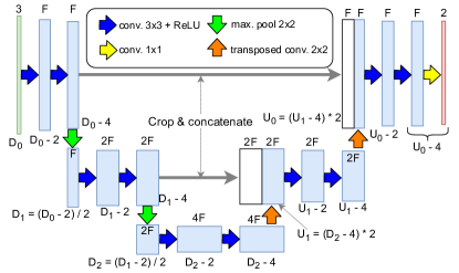
Figure 4: Architecture of a 3 layer U-net for binary classification of 3-channel images. At level $k$, the layers undergo convolution with a series of 3x3 filters, producing $2^{k}F$ feature maps. The initial size $D_{0}$ of the input image is approximately halved at each downsampling layer, an approximately doubled in each upsampling layer (up to border removing convolutions). The final layer is obtained by a 1x1 convolution with the top-level upsampled feature layer, and is subsequently fed into the softmax operator to derive class posterior probabilities.

4.2 Image intensity prior

In the role of the image intensity prior $P_{i}(C|I)$ for our target class of fallen trees, we utilize the U-net deep neural network 4.1 in a binary classification setting. The original architecture is easily adaptable to the variable number of input channels $N_{c}$. The per-pixel posterior object class probabilities conditioned on the image pixel intensities (i.e.$P_{i}(C|I)$) are obtained directly from the semantic segmentation. We subsequently apply the marching squares algorithm (Lorensen and Cline, 1987) to derive contours of $q-$level supersets of the probability image. This results in a set of high-probability polygons, possibly consisting of multiple fallen trees and non-class objects or noise. Since the best known geometric algorithms used for calculating polygon intersections have a worst-case computational complexity proportional to the product of their vertex counts in the general (non-convex) case (Nievergelt and Preparata, 1982), we apply the contour simplification algorithm by Douglas and Peucker (1973) (parameterized by the max. simplification distance $\epsilon_{d}$) to the polygons, resulting in the final set $S$ defined in Sec. 3.

4.3 Shape generator

As the shapes of fallen stems are well approximated by rectangles, we utilize a simple shape generator $f_{s}(\bar{\alpha})$ parameterized by two scalars $\alpha=[a,b]$, which produces a rectangle with side lengths $a,b$ centered at the origin of the coordinate system, oriented parallel to its axes (i.e. in standard position):

$$\begin{split}&f_{s}(a,b)=[(-\frac{a}{2};-\frac{b}{2}),(\frac{a}{2};-\frac{b}{2}),(\frac{a}{2};\frac{b}{2}),(-\frac{a}{2};\frac{b}{2})]\\ &f_{s}(a,b;\theta=[x_{c},y_{c},\rho])=R_{\rho}f_{s}(a,b)+T_{x_{c},y_{c}}\end{split}$$ (7)

The rigid transformation parameters $\theta$ consist of the center position $(x_{c},y_{c})$ translation $T$ and an in-plane rotation $R$ by angle $\rho$.

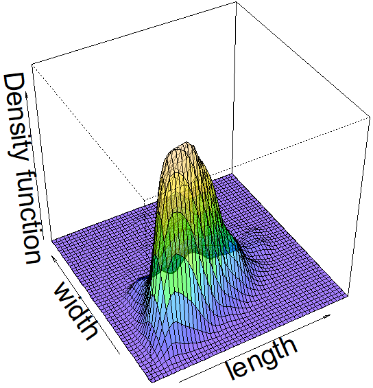
Figure 5: Sample kernel density estimator model of joint stem length/width probability based on reference labeled polygons.

4.4 Energy components

Here we provide details about component potentials of the energy function (Eq. 1). Aside from the 3 standard potentials defined in Section 3, we introduce an auxiliary collinearity potential to help prevent the fragmentation of object detections into multiple collinear parts.

4.4.1 Data fit and overlap terms

We utilize the aforementioned (Sec. 3.3) second-order inclusion-exclusion principle based formulation to approximate the set difference cardinalities $\phi\setminus\tau,\tau\setminus\phi$ by appropriate pairwise intersections. Since the model polygons have a constant dimension of 4 vertices, the computation of any pairwise intersection of model polygons $i$ and $j$, $f_{s}(\alpha_{i}|\theta_{i})\cap f_{s}(\alpha_{j}|\theta_{j})$ may be done in constant time, whereas the computational complexity of intersecting any $f_{s}(\alpha_{i}|\theta_{i})$ with a high-probability contour $s_{i}\in S$ is linear in the number of vertices forming $s_{i}$ (Nievergelt and Preparata, 1982). Additionally, we modify the generic overlap potential $E_{o}$ (Eq. 3) to include a dependency on the angular difference in orientations between the model shapes:

$$E_{o}(i,j)=e^{\frac{-(\rho_{i}-\rho_{j})^{2}}{2\sigma_{o}^{2}}}|f_{s}(\alpha_{i}|\theta_{i})\cap f_{s}(\alpha_{j}|\theta_{j})|$$ (8)

This reflects the model’s capability to allow non-parallel, crossing shapes to overlap without being penalized, as they most likely do not correspond to the same object (fallen stem).

4.4.2 Shape prior

We utilize a shape prior model in the form of a kernel density estimator defined on the shape coefficients $\bar{\alpha}=[a,b]$, based on a set of training rectangle shapes $S_{T}=\{\bar{\alpha}_{k}\}$:

$$P_{s}(\bar{\alpha})=\frac{|H|^{-1/2}}{|S_{T}|}\sum_{k=1}^{n}K(H^{-1/2}(\bar{\alpha}-\bar{\alpha}_{k}))$$ (9)

In the above, the bivariate Gaussian kernel is applied in the role of $K$, whereas the bandwidth matrix $H$ is determined via the plug-in selection method of Wand and Jones (1994). A sample shape model derived from part of our reference shapes is depicted in Fig. 5.

4.4.3 Collinearity prior (auxiliary potential)

While the overlap penalty will discourage the formation of highly overlapping model shapes, there is still a possibility of segmenting a single tree stem as a sequence of nearly-collinear parts (see Fig. 6). To mitigate this, we introduce an auxiliary pairwise collinearity potential $E_{c}=\sum_{i,j}E_{c}(i,j)$, which penalizes highly collinear shapes located in close proximity with each other. Here, we define $E_{c}(i,j)=\log P_{eq}(f_{s}(\alpha_{i}|\theta_{i}),f_{s}(\alpha_{j}|\theta_{j}))$ as the log-probability $P_{eq}$ of the two shapes $i,j$ belonging to the same stem. In practice, we use the output of a probabilistic classifier (e.g. logistic regression) acting on differential features derived from the shapes’ locations (angular deviation of orientations, mean average distance of central axes). This is in analogy to the object similarity function applied to graph cut segmentation of stem parts into individual fallen trees defined in our prior work (Polewski et al., 2015a). However, the log-probability contributes positive values to the energy for each detected collinear shape pair, thereby biasing the model away from such states and encouraging a merge operation of the interacting shapes.

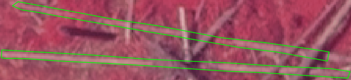
(a)

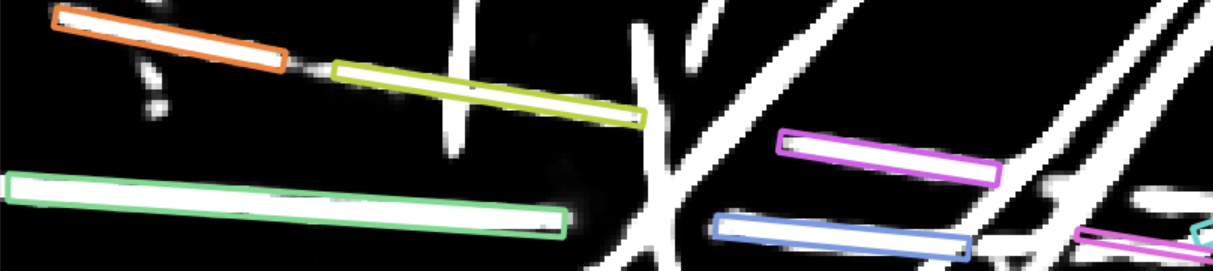
(b)

Figure 6: (a) Color infrared image of forest scene with fallen stems. Two long stems are marked with green outlines. (b) Sample detection result for the two stems over posterior class probability image of same scene. Due to occlusions, the stems are fragmented and discontinuous within the probability map, which causes the energy function to prefer multiple disconnected collinear fragments over a single polygon covering the full length of the stem.

4.5 Initialization with sample consensus

We initialize our model with a set of line segments automatically detected using sample consensus (SAC) methods (Fischler and Bolles, 1981) within the binarized probability image $P_{i}(C|I)$ obtained from semantic segmentation (see Sec. 4.2). The inlier threshold for $d_{sac}$ SAC is set to the maximum expected width of a fallen stem (expressed in pixels). We only allow line segment hypotheses having a minimal length $l_{sac}$, again derived from the minimal length of a tree stem we expect to find. This segment length is measured as the length of the interval of inlier pixel projections onto the respective model line. We also impose a minimum number of inlier points $n_{sac}$ for valid hypotheses. The whole scene is processed iteratively, greedily picking the highest-inlier hypothesis until there are no valid hypotheses left. We expect to discover an overabundance of line segment hypotheses, partially covering the vast majority of true stem segments within the scene (see Fig. 7). Each accepted SAC hypothesis becomes an initial model shape, with the length $l_{0}^{i}$ and position $t_{x,0}^{i},t_{y,0}^{i}$ / orientation $\rho_{0}^{i}$ inherited from the SAC line and a default assigned width. It is up to our energy formulation to eliminate redundant model elements, determine true dimensions of each object, and improve delineation of individual stem boundaries.

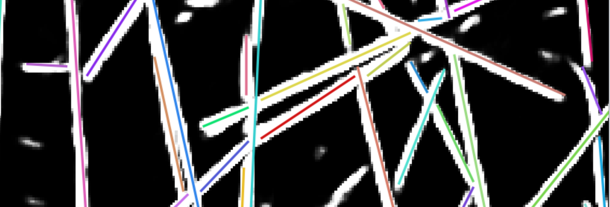
Figure 7: Line segments discovered using an iterative sample consensus (SAC) method. Although most target class pixels are covered by at least one SAC line, the method usually overestimates the true number of stems due to the variability of stem width distributions and the resulting difficulty in defining a single inlier threshold appropriate for all cases.

4.6 Efficient evaluation of neighboring solutions

As our fallen tree detection pipeline is designed for processing high-resolution nadir-view aerial imagery, it seems reasonable to quantize some size and position parameters at the ground sampling distance (GSD) of the input image, i.e. the finest level of detail available within the image. Given the elongated shape of our target objects (fallen tree stems), this quantization can yield a significant reduction of some parameters’ domains. Specifically, assuming a typical GSD of high-resolution aerial imagery of 5-10 cm, and the diameter of fallen stems bounded by 70 cm, the width parameter of the generated rectangle would only admit a small number (7-14) of possible values. For this reason, we restrict the elements $a,b$ of the shape coefficient vector $\bar{\alpha}$ and to the integer domain, representing the number of pixels at the original image resolution. The rectangle length and width $a,b$ are additionally equipped with their own lower/upper bounds $[a_{lo};a_{hi}],[b_{lo};b_{hi}]$ based on the image resolution and the expected maximum/minimum stem dimensions. The lower bound $b_{lo}$ of the width is set to zero, which allows the model to ’disable’ a particular, redundant shape altogether and prevent it from contributing to the energy function (through zero overlap with any other polygons). Additionally, we impose restrictions on the location of the centers $t_{x}^{i},t_{y}^{i}$ for every shape $i$ separately, based on the centers of their SAC line segment initializations $t_{x,0}^{i},t_{y,0}^{i}$ (see previous section). The center of the model shape $t_{x}^{i},t_{y}^{i}$ must be located within a rectangle of length $l_{0}^{i}$ oriented according to the initial SAC angle $\rho_{0}^{i}$ and having a width $w_{0}$ which is a parameter of our method (see Fig. 8). We introduce these constraints in order to avoid drifting away from the initial SAC solutions into poor regions of the solution space where no overlap of model objects with high probability level-supersets of the image would exist and hence loss of gradient would occur. The optimization method of choice, simulated annealing, is susceptible to this kind of behavior during the initial phases of the minimization process, where the temperature parameter remains high and even poor moves which deteriorate the solution quality continue to be accepted.

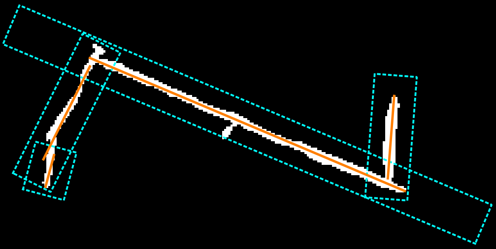
Figure 8: Probability image with detected initial sample consensus hypotheses (orange lines). Each line is surrounded by its center constraints polygon (cyan boxes). The evolution of the model shape associated with the given hypothesis line is constrained to maintain the center of the shape within the corresponding box at all times.

4.6.1 Solution altering moves

Consider the state $\Omega^{k}$ of the solution at iteration $k$ of the optimization process, consisting of all shape and rigid transformation parameters concatenated into a single vector: $\Omega^{k}=(\omega_{i}^{k}=(\bar{\alpha}_{i}^{k},\theta_{i}^{k}))$ (see Sec. 3.1). To generate a new candidate state $\Omega^{k+1}$ from $\Omega^{k}$, we designed the following solution altering moves, acting on a random shape $\omega_{u}^{k}$:

1. length/width: add/subtract a random integer bounded by $\delta_{l},\delta_{w}$ respectively to the length/width of shape $u$

2. angle: add/subtract a random real number bounded by $\delta\rho$ to the angle $\rho_{u}$ related to shape $u$’s orientation

3. location (along axis): shift the center of shape $u$ along its current axis by a random number bounded by $\delta_{t,ax}$

4. location (arbitrary): shift the center of shape $u$ by an arbitrary random 2D vector, the components of which are bounded by $\delta_{x},\delta_{y}$

5. merge/absorb: for a collinear shape $\omega_{v}^{k}$, extend the shape $u$ by projecting the vertices of both shapes onto the current axis of shape $u$ and adjusting its length and center point such that $u$ contains all the projections. Also, disable the contributions of shape $v$ to the overall energy by setting its width to zero

The selection of the move to apply is based on a uniform random choice, where the merge/absorb move is only considered if the probability $P_{eq}$ of two shapes belonging to the same object is above a threshold value (see Sec. 4.4.3). Moves (i)-(iv) are of a local nature in the sense that only the model shape $u$ changes. To calculate the new energy, we only need to perform a series of constant-time rectangle intersection computations between $u$ and the remaining shapes, as well as one or more intersection calculations between $u$ and the high-probability object contours $s\in S$, linear in the respective vertex counts. The values of the remaining model shape and image contour intersections remain unchanged and can be cached as described in Sec. 3.3. In case of move type (v), a similar technique can be applied, because while technically two shapes are altered, only the ’absorbing’ shape $u$ needs to have its intersections recalculated since shape $v$ becomes an empty contour whose intersection with an arbitrary polygon yields the empty set.

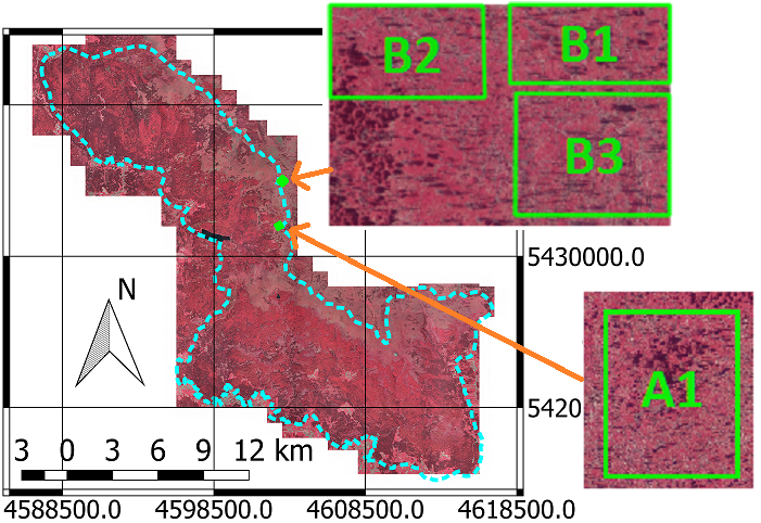
(a)

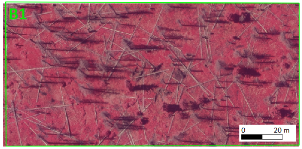
(b)

Figure 9: (a) Training and validation regions (in green) chosen within the Bavarian Forest National Park (boundaries shown with dashed cyan line). The coordinates and true north arrow are with respect to the coordinate reference system DHDN/3-degree Gauss-Krüger zone 4 (EPSG:31468). Background is color infrared image with ground sampling distance of 10 cm. Region A was used exclusively for training, whereas region B was the basis for validation. (b) a depiction of test area B1, containing a mixture of lying dead trees, standing dead trees, and living vegetation.

5 Experiments and results

In this chapter, we describe the source imagery, target training and test areas, reference data, evaluation strategies, and the details of our experimental setup used to evaluate the proposed dead tree delineation framework against a baseline method. We also list the principal numerical results.

5.1 Data acquisition

For validating our method, we utilized aerial imagery from the Bavarian Forest National Park, situated in South-Eastern Germany ($49^{\circ}3^{\prime}19^{\prime\prime}$ N, $13^{\circ}12^{\prime}9^{\prime\prime}$ E). The Bavarian Forest lies in the mountain mixed forests zone consisting mostly of Norway spruce (Picea abies) and European beech (Fagus sylvatica). From 1988 to 2010, a total of 5800 ha of the Norway spruce stands died off because of a bark beetle (Ips typographus) infestation (Lausch et al., 2013). Color infrared images were acquired in the leaf-on state during a flight campaign carried out in June 2017 using a Leica DMC III high resolution digital aerial camera with a nadir across track field of view of 77.3^∘ (see Leica (2017) for the product sheet). Multiple multispectral color cameras were utilized to form composite images, which had a resolution of 14592 x 25728 pixels with a virtual pixel size of 3.9 $\mu m$ on the CMOS sensor. The mean above-ground flight height was ca. 2879 m, resulting in a pixel resolution of 10 cm on the ground. The flight campaign took place between 10:30 and 13:25, with the sun’s position traversing the range 49^∘64^∘35^∘. The images contain 3 spectral bands: near infrared (spectral range 808-882 nm), red (619-651 nm) and green (525-585 nm). All digital CIR images were radiometrically corrected by using optimal camera calibration observations, transformation parameters and ground control points. The procedures were conducted in the program system OrthoBox (Orthovista, Orthomaster) of the company Trimble/INPHO.

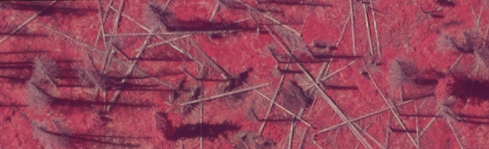
(a)

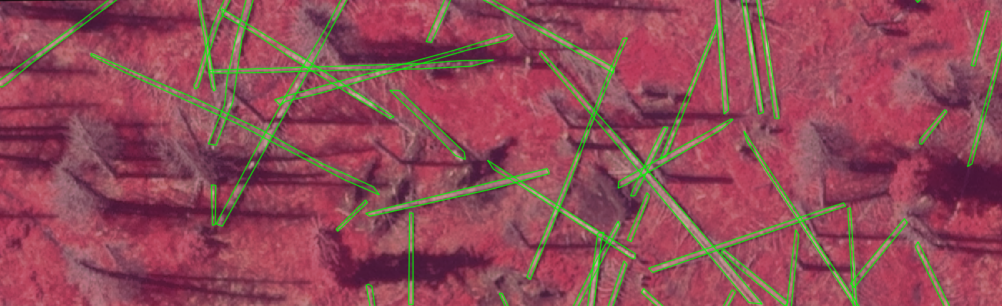
(b)

Figure 10: (a) Sample color infrared (CIR) image containing fallen stems. The ground sampling distance of 10 cm is sufficient to delineate each individual stem with high precision (b).

5.2 Reference data

Two separate regions of the National Park were used in this study (Fig. 9). We manually labeled individual stems forming large groupings of fallen trees visible in the high-resolution aerial imagery (Fig. 10). We only considered stems with a minimal length of 2 m. In Region A, a total of 213 single stem polygons were labeled. These polygons formed the basis for training the semantic segmentation component (U-net, see Sec. 5.4.1). Additionally, we used Region B, disjoint from Region A, to derive a total of 730 fallen tree polygons distributed across 3 test areas (Fig. 9). We took care to mark all visible fallen stems in each respective area to enable a fair evaluation. The areas B1, B2, and B3 are ordered by an increasing, subjective degree of segmentation difficulty. The first test area (B1) comprises 157 fallen stems and a number of standing dead trees in a state of advanced decay (Fig. 9(b)), distributed over an area of 140 x 70 $m^{2}$. The fallen trees are often Area B2 is slightly larger with dimensions of 140 x 70 $m^{2}$, but contains significantly more stems with a count of 218. It contains some visually more challenging scenarios of many stems intersecting at various angles. Finally, area B3 (140 x 107 $m^{2}$) is the most challenging among the test plot, with 355 fallen stems and difficult scenarios of many stems forming complex interactions. A particularly dense region within area B3 is depicted in Fig. 12.

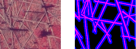
(a)

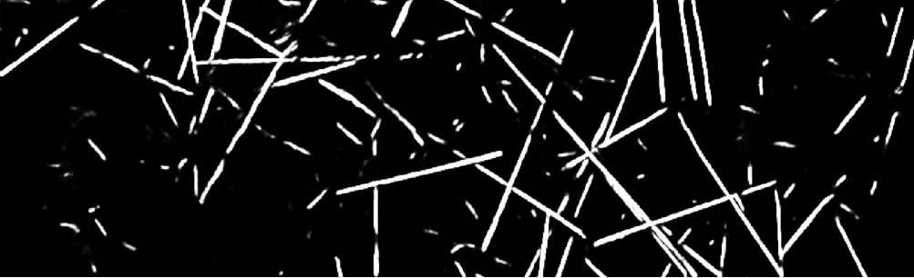
(b)

Figure 11: (a) an image patch for U-net training. left: original CIR image, right: pixel mask showing target class (magenta) and non-class (blue) pixels. The black regions within the image do not contribute to the training loss function, which enables the learning to focus more on the boundary between the stem and its surroundings. (b) Per-pixel probability of belonging to a fallen stem, obtained from semantic segmentation with the trained U-net.

5.3 Evaluation criteria

We utilize two classic measures, correctness (also known as precision/specificity) and completeness (recall/sensitivity) to quantify the detection and segmentation results. We instantiate these measures in two complementary settings: (i) polygon level and (ii) centerline level. In both scenarios, correctness is conceptually defined as the ratio of detected objects which may be linked to reference stems, whereas completeness refers to the converse: the ratio of reference stems which have a detected counterpart. The exact matching criteria for the polygon versus the line case are listed below.

5.3.1 Polygon level

This version of the evaluation criteria is used for comparing the polygons delineated by our method versus the manually created reference polygons. To consider a reference polygon $r$ as matched, we require that there exist a detected polygon $d$ such that $|r\cap d|/|r|>0.5$, i.e. more than half the area of $r$ must be covered by the detection. Similarly, the matching criterion for a detected polygon $d^{\prime}$ is the existence of a reference polygon $r^{\prime}$ such that $|r^{\prime}\cap d^{\prime}|/|d^{\prime}|>0.5$. Using basic algebra of sets, it’s possible to show that these conditions taken together guarantee an intersection-over-union (IoU) value above $1/3$. While an IoU value of 0.5 is often regarded as the cutoff point for ’good’ detection, there are several reasons why we chose a smaller threshold: (i) the polygons represent the objects themselves, not bounding boxes like in a typical detection scenario, (ii) some fallen stems marked as whole within reference data may be fragmented into multiple parts by shadows within the image, thereby making detection with a single contiguous polygon unlikely, and (iii) the detected polygons are typically only several pixels wide, so an error in width of merely 1 pixel could result in a significant loss of overlap area (e.g. 15% or more). We report the mean IoU values on matched reference stems for relevant experiments.

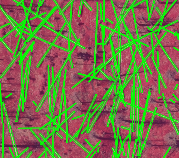
Figure 12: Dense region within plot B3, where many stems are concentrated on a relatively small area.

5.3.2 Line level

Since the baseline method for comparison (i.e. sample consensus line detection) does not produce polygons, we introduce the line-based evaluation for the sake of fairness. Similar to the polygon case, we perform pairwise comparisons between line segments extracted from the reference and detected polygons. The segments for the reference polygons are derived from the centerlines of their oriented bounding boxes, whereas for the detected rectangles they are simply the centerlines parallel to the longer rectangle edge, clipped to lie within the shape. To determine a match between two segments, we adapt the 3D matching criterion from our prior work concerning detection of fallen stems in point clouds (Polewski et al., 2015a) to the 2-dimensional case. Let $\vec{r},\vec{d}$ denote, respectively, the reference and detected line segments which are candidates for matching. We consider $\vec{r}$ matched with $\vec{d}$ if and only if the following 3 criteria are met (see Fig. 13):

• the angular deviation between $\vec{r},\vec{d}$ is below $5^{\circ}$

• the mean projected distance between $\vec{r},\vec{d}$ is below 35 cm, or half-width of the average stems we expect to encounter

• the projection of $\vec{r}$ onto $\vec{d}$ must have a minimum length of 60%$\cdot|\vec{d}|$

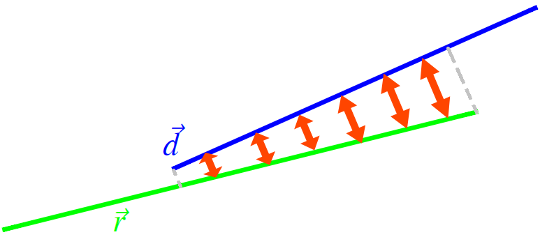
Figure 13: Computing the average projection distance and cover between two line segments $\vec{d},\vec{r}$. The average distance is taken over a discrete set of projected points (orange distance markers). Dashed gray lines indicate the region of $d$ covered by the projection of $r$ onto $d$.

	Collinearity coefficient
	Polygon level								Line level
	Off		Low		Mod.		High		Off		Low		Mod.		High
Precision/recall	P	R	P	R	P	R	P	R	P	R	P	R	P	R	P	R
Shape coefficient
Plot B1
Off	.90	.81	.90	.80	.91	.82	.90	.80	.88	.76	.89	.74	.89	.76	.88	.75
Low	.90	.81	.90	.82	-	-	-	-	.88	.75	.88	.77	-	-	-	-
Mod.	.90	.82	-	-	.91	.82	-	-	.89	.75	-	-	.88	.76	-	-
High	.90	.82	-	-	-	-	.89	.80	.87	.75	-	-	-	-	.86	.73
Plot B2
Off	.91	.73	.93	.73	.92	.74	.92	.72	.87	.73	.88	.73	.88	.75	.87	.73
Low	.92	.75	.92	.74	-	-	-	-	.87	.75	.87	.73	-	-	-	-
Mod.	.93	.75	-	-	.92	.75	-	-	.87	.74	-	-	.87	.74	-	-
High	.91	.77	-	-	-	-	.91	.76	.87	.74					.87	.73
Plot B3
Off	.93	.76	.93	.77	.93	.78	.93	.78	.89	.77	.89	.78	.88	.79	.89	.78
Low	.93	.77	.92	.78	-	-	-	-	.88	.76	.89	.78	-	-	-	-
Mod.	.93	.78	-	-	.91	.78	-	-	.88	.76	-	-	.88	.78	-	-
High	.93	.79	-	-	-	-	.93	.79	.87	.75	-	-	-	-	.87	.77

Table 1: Sensitivity analysis results for the influence of the shape and collinearity energy potentials onto the aggregate energy. Precision and recall of the detection are given for both the polygon- and line-level evaluation. Four levels of influence are investigated for each potential, where ’off’,’low’,’moderate’,’high’ correspond respectively to term coefficient values of $0,0.1,0.3,0.5$ within the aggregate energy. The energy term coefficient configurations yielding the highest precision (correctness) are emphasized with bold font (recall value breaks ties).

5.4 Experimental setup and results

We performed a number of computational experiments to determine both the absolute performance of the entire processing pipeline, its relative performance versus a sample consensus baseline, as well as the influence of its components on the detection quality. To facilitate computations and enable concurrent processing, each high-probability polygon obtained from the U-net semantic segmentation (Sec. 4.2) is considered independently. In all experiments, the data fit coefficient $\gamma_{d}$ was kept constant at $\log\epsilon,\epsilon=1e-6$. Moreover, the overlap potential $E_{o}$ is measured in the same units (i.e. polygon area) as the data fit term, therefore we also set $\gamma_{o}=\gamma_{d}$ to maintain the same semantics of an area unit in both potentials. The setting of $\epsilon$ assumes that the target class probability of pixels outside and inside the selected image regions is respectively $1e-6,1-1e-6$. In fact, all three of the quantities $E_{d},E_{s},E_{o}$ may be interpreted as (log-)probabilities, and we make use of this fact to define a simple potential normalization scheme. This is to promote interpretability of the energy coefficients $\gamma$, such that potentials having similar coefficient values will also exert a similar influence on the energy function. In particular, we divide each potential by the cardinality of the set it was integrated over, so that $E_{d}$ is divided by the area of the currently processed high-probability polygon $s\in S$, $E_{s}$ is normalized by the number of evolving shapes $M^{\prime}$, whereas the normalization constant for $E_{c}$ is the number of unordered pairs $\binom{M^{\prime}}{2}$.

The simulated annealing was carried out with 16 random restarts, picking the result with the best objective function value. The number of inner iterations per temperature level was 15000, and the cooling factor was set to 0.9. The minimum and maximum accepted stem length was 2 m and 30 m, respectively. Detected polygons with lengths outside this interval were discarded.

To gain a deeper insight into the experimental results, we partitioned the set of reference trees per plot into two categories, based on their overlap with other reference polygons. Standalone objects not intersecting any other stem were considered ’simple’, whereas stems belonging to groupings of mutually overlapping polygons were categorized as ’complex’. The percentages of reference trees classified as ’complex’ in the test areas B1, B2, and B3 were respectively 53%, 59%, and 69%.

5.4.1 Training the U-net

We utilized the manually marked stem polygons to train an instance of the 3 layer U-net depicted in Fig. 4, with additional dropout and batch normalization layers. The implementation provided by Akeret et al. (2017) was adapted to our data. The input image size $D_{0}$ was 200 pixels, and the number of features (convolutional filters) at top level was set to $F=32$. Since stems are elongated thin structures, usually the proportion of pixels occupied by them is small compared to the background. Therefore, we only used pixels lying within a small 4-pixel band around the marked stem polygons in the role of negative class examples. This was to enhance the class balance and also encourage the learning process to focus on learning the boundaries between stems and their immediate surroundings instead of random background patterns (Fig. 11(a)). The resulting class label distribution was imbalanced with 31% of pixels representing fallen stems. A sample result of the probabilistic output obtained from semantic segmentation with the trained U-net is shown in Fig. 11(b). We used the Adam algorithm (Kingma and Ba, 2017) to perform stochastic gradient optimization of a binary logistic objective until convergence. Standard metaparameters for the Adam optimizer were assumed ($\alpha=0.001,\beta_{1}=0.9,\beta_{2}=0.999$). The dropout rate was 50 %, whereas the training minibatch size was set to 15.

5.4.2 Sensitivity analysis for energy coefficients

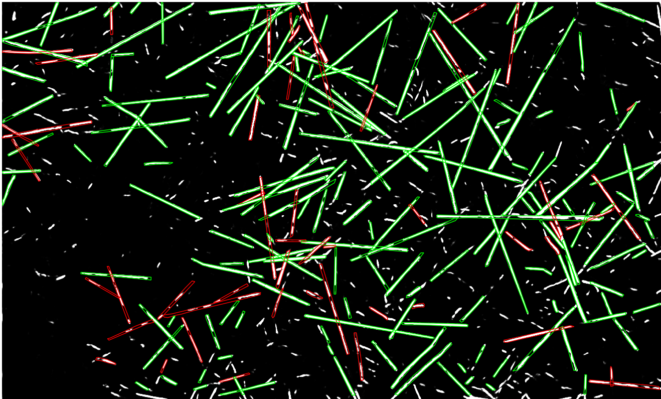
(a)

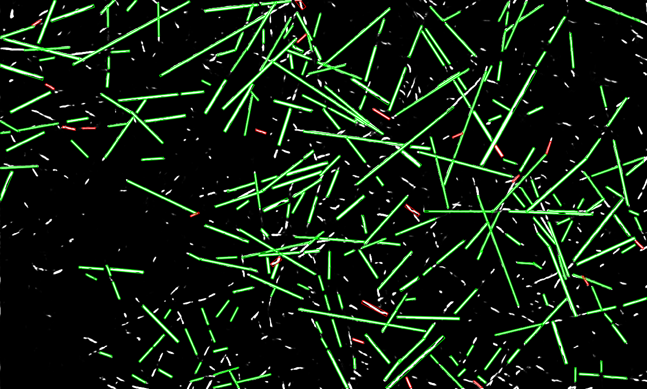
(b)

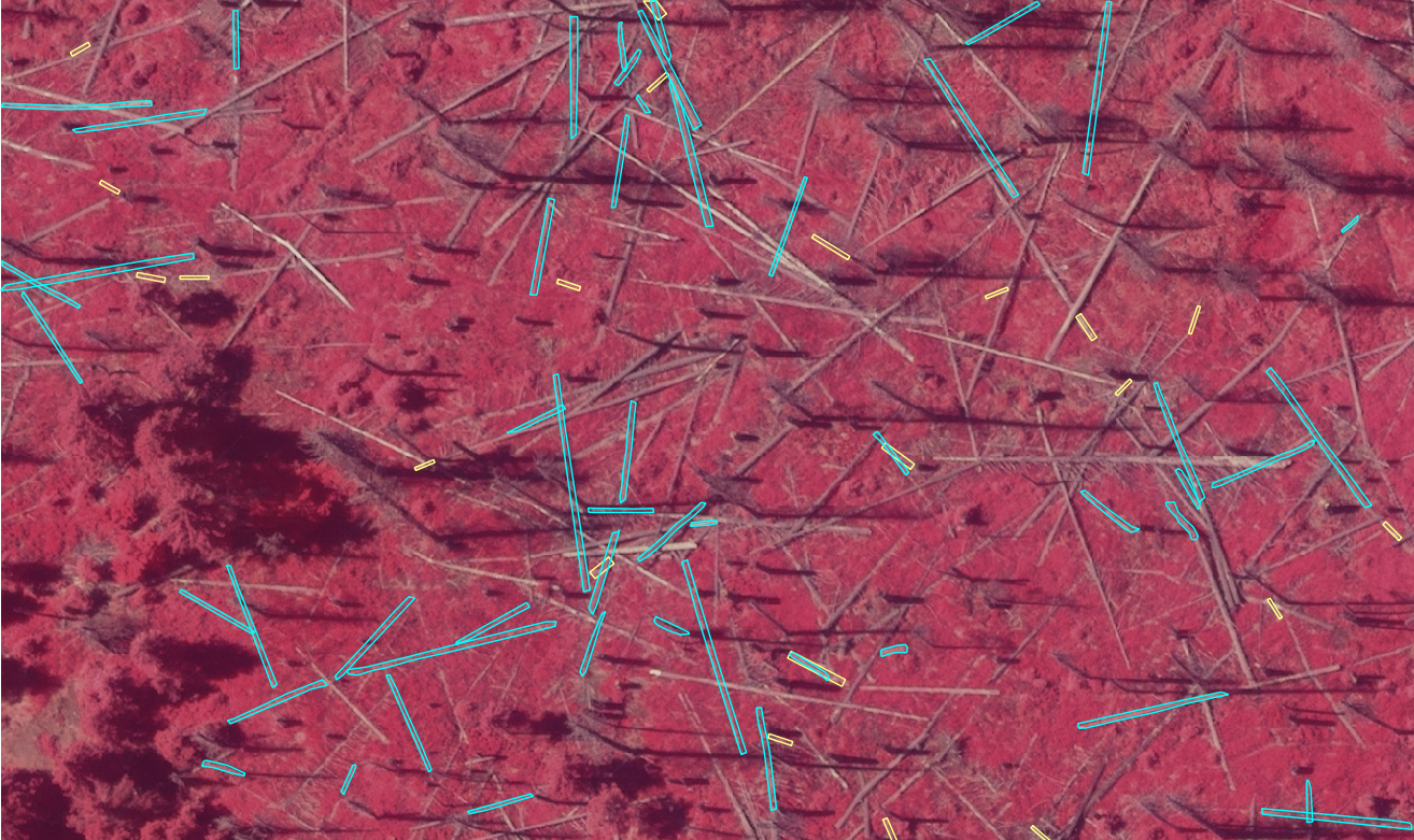
(c)

Figure 17: Results of fallen stem segmentation for plot B2 (polygon level). (a), (b) depict respectively the reference and detected polygons, with semantic segmentation posterior probability as background. Red/green colors indicate a polygon mismatched/matched with a counterpart (above 50% area overlap). (c) original false color CIR image with indicated mismatched reference (cyan) and detected (yellow) polygons.

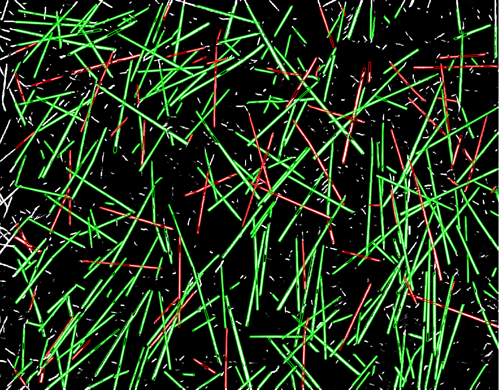
(a)

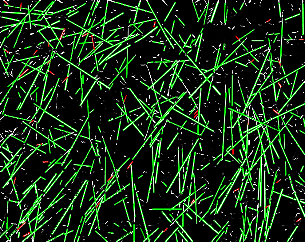
(b)

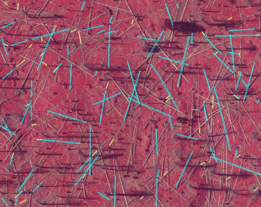
(c)

Figure 18: Results of fallen stem segmentation for plot B3 (polygon level). (a), (b) depict respectively the reference and detected polygons, with semantic segmentation posterior probability as background. Red/green colors indicate a polygon mismatched/matched with a counterpart (above 50% area overlap). (c) original false color CIR image with indicated mismatched reference (cyan) and detected (yellow) polygons.

In the first experiment, we varied the energy coefficients $\gamma_{s},\gamma_{c}$ corresponding respectively to the shape and collinearity energy terms $E_{s},E_{c}$ (Secs. 4.4.2,4.4.3). Thanks to the normalization scheme described above, it suffices to investigate coefficient values of the order of magnitude $1$. We introduced 4 levels of coefficient magnitude: $(0,0.1,0.3,0.5)$, corresponding to labels of $L=$off,low,moderate,high. Performance metrics were collected for the following combinations of $(\gamma_{s},\gamma_{c})$: $\{(\text{off},\text{off})\}\cup\{\{(\text{off},x),(x,\text{off}),(x,x)\}:x\in L\}$. For the polygon-based evaluation, we recorded the correctness and completeness as per Sec. 5.3.1 as well as the mean matched intersection-over-union measure. In case of line-based evaluation, the metrics saved were (i) the correctness and (ii) a version of completeness which considers only reference stems which were covered by detected segments (in the projection sense, see Fig. 13) to a degree of at least 65%. The results are summarized in Table 1. Also, Figs. 16-18 visualize the detection results of the best performing parameter combinations for the 3 target areas. On the polygon level, a correctness above 0.9 was reached for all plots, with completeness values between 0.77 and 0.82. The highest attained intersection-over-union was 0.59, 0.55, and 0.58 respectively for plots B1, B2, B3. The plot exhibiting the highest completeness was also the one with the highest percentage of ’simple’ (single component) reference trees. Adjusting the shape and collinearity term coefficients yielded an improvement in precision/recall of 1/1, 2/4, and 0/3 percentage points (pp) respectively for plots B1, B2, B3. Moreover, all results with the highest attained correctness were associated with a ’moderate’ or higher shape term coefficient. In contrast, varying coefficients did not influence the line level evaluation much, with precision/recall gains of 1/0, 1/2, and 0/1 pp. Overall, relative to the polygon level, the line evaluation resulted in slightly lower values for precision at 88-89 and completeness of 75-78.

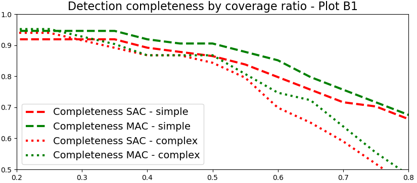
(a)

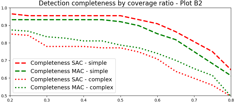
(b)

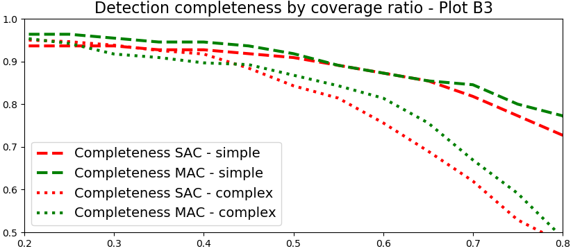
(c)

Figure 14: Detection completeness results for the 3 test plots - comparison between the sample consensus baseline (SAC) and our multiple active contour (MAC) method. The horizontal axis indicates the ratio of the reference tree’s length which is covered by the projection of its matched detected line. A point $(p,q)$ on the plot is interpreted as $q$ of all reference trees having a valid match which covers at least $p$ of their length.

5.4.3 Comparison to baseline (sample consensus)

The purpose of this experiment was to compare the line-based detection quality to the sample consensus baseline. To this end, we executed the sample-consensus based line segment detection within the high-probability components from U-net semantic segmentation (Sec. 4.5), and considered the SAC line segments as the final detection result. To account for randomness and to equalize the chances versus the compared-to method, the SAC computations were repeated a number of times equal to the size of checked coefficient combination set in the first experiment, and the best result was noted. We then picked the best-performing coefficient combination per plot as per Table 1 and performed a more in-depth comparison of our method and the SAC result using more metrics. Notably, we analyzed completeness at different thresholds of stem coverage as well as correctness of detecting ’simple’ stems (which occupy their individual input polygon, without intersecting other trees) versus ’complex’ stems (which are part of a complex aggregate of multiple overlapping objects). The curves showing detection completeness as a function of reference stem projected coverage ratio are depicted in Fig. 14, whereas the remaining metrics are given by Table 3. In terms of overall precision (correctness), our method attains a lead of 4 pp consistently across the test plots. However, considering the complexity of the reference stems, this difference is extended to 5-7 pp for complex stems and reduced to 0-3 pp for simple (single component) stems. The detection completeness (recall) follows a similar trend, with our method outperforming the baseline by up to 5 pp for simple and up to 7 pp for complex stems. Note that the advantage of our method becomes more clear at coverage levels beyond 60%, whereas for low coverage levels, both methods perform similarly.

5.4.4 Comparison to semantic segmentation baseline - logistic regression

This experiment involved replacing the high-quality semantic segmentation probability map from the U-Net with a basic logistic regression model trained only on the channel intensities. The same data was used for training both models. No higher-level textural features were used in order to determine the benefit of using a state-of-the-art neural network for semantic segmentation. The pixel-level classification accuracy and F1 score on a hold-out validation set for the U-Net were respectively 0.94 and 0.91. The cross-validated overall accuracy and F1 score for the logistic regression baseline attained values of 0.80 and 0.62. We then applied the logistic regression model to the images of the test area, obtaining maps of posterior class probabilities. Polygons of high probability regions were subsequently extracted and our multi-contour segmentation was executed. Although the per-pixel classification metrics for the logistic regression were satisfactory, the object-level (both line and polygon) performance appeared to break down. The precision degraded to levels of 0.76-0.83, and the recall experienced an even more extreme drop to levels of 0.15-0.27. In Fig. 15, the semantic segmentation of the same area by the LR baseline and by the U-Net is shown. It can be seen that within the LR probability image, many stems are missing or greatly ’thinned out’, i.e. represented by only a sparse set of pixels.

5.5 Execution time

The training process of the U-net on an nVidia GeForce GTX 1080 Ti graphics card (with CUDA support) took ca. 7.5 hours, after which time convergence of the learning process was achieved. The prediction time of the U-net on new data was measured in seconds and negligible compared to the optimization time of the multi contour objective. This optimization was carried out on a desktop computer equipped with 128 GB of RAM and an Intel XEON E5-1680 v4 CPU running at a frequency of 3.4 GHz, consisting of 8 cores. We used our own implementation of the simulated annealing metaheuristic algorithm written in the C++ programming language. The mean execution times of the inference/optimization on the respective test areas (averaged over different choices of the objective function parameters $\gamma_{s},\gamma_{c}$) are given in Table 2.

	Plot B1	Plot B2	Plot B3
Mean exec. time [h]	3.95	6.68	13.46
Standard dev. [h]	0.17	0.42	0.46
Time per stem [s]	61	83	91

Table 2: Execution times of simulated annealing based optimization of proposed multi active contour method on the 3 test areas. The shown values correspond to the mean execution time, standard deviation, and mean time for processing one stem per test area.

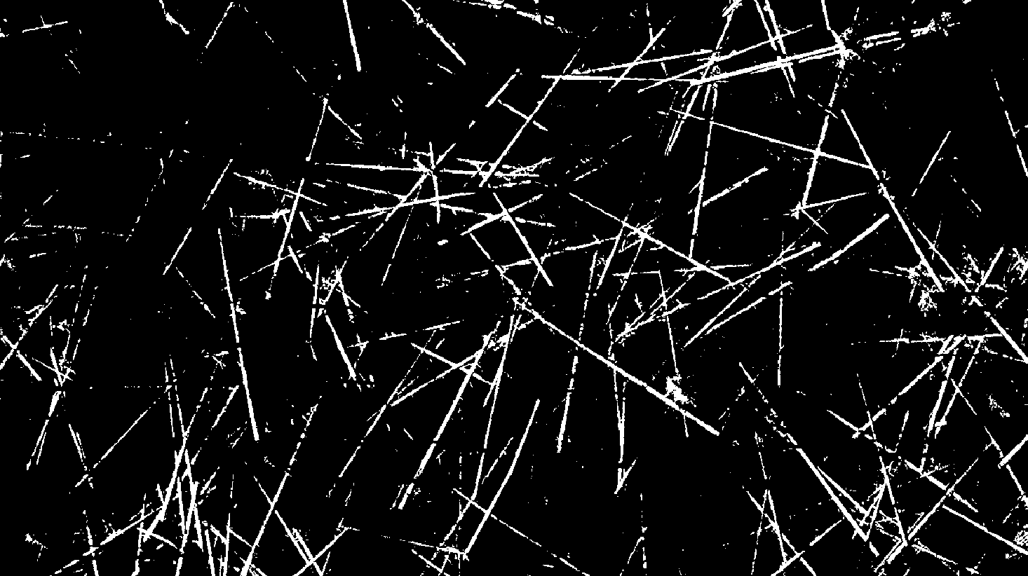
(a)

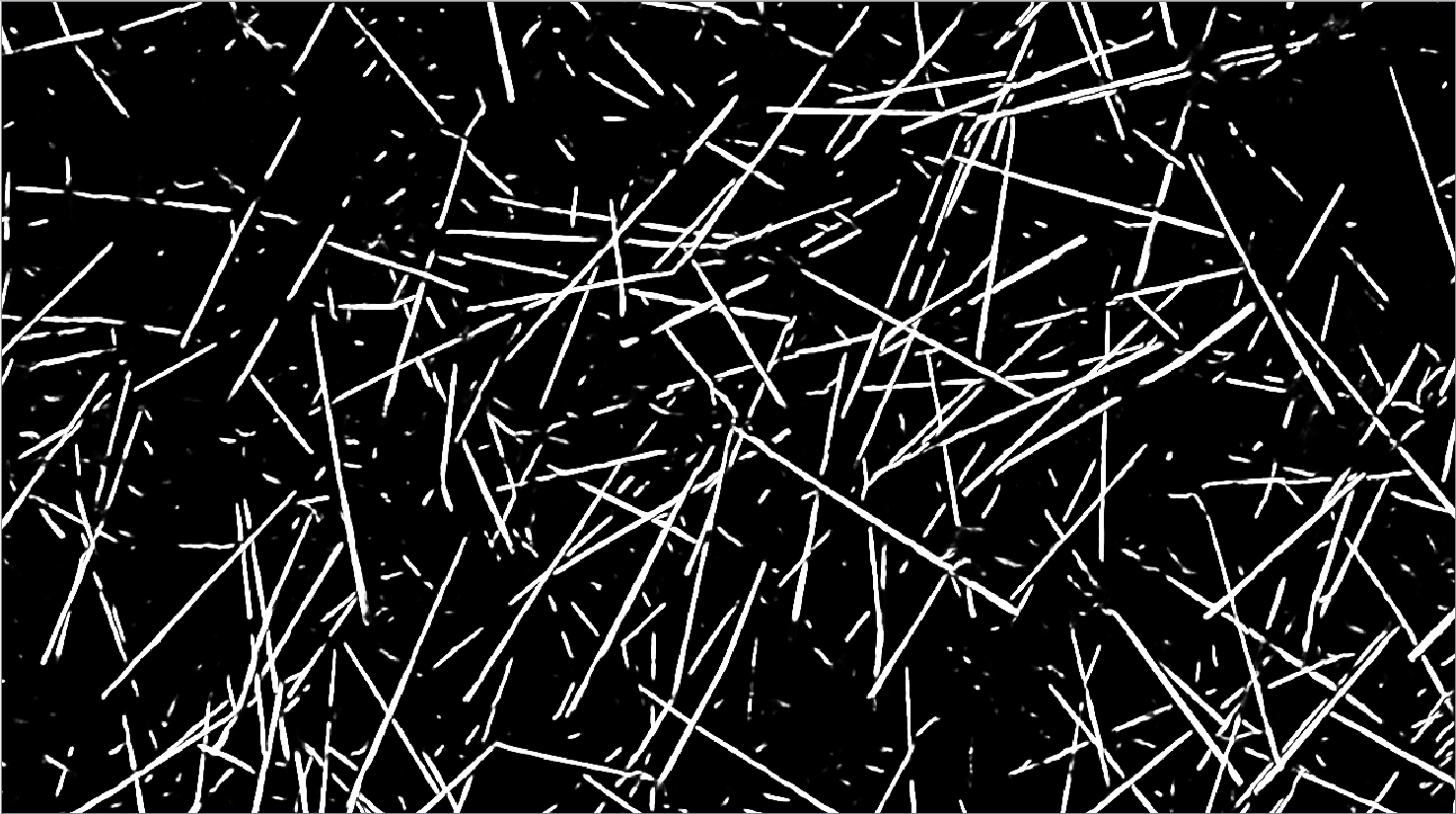
(b)

Figure 15: Comparison of posterior probabilities from semantic segmentation by (a) logistic regression based on simple channel intensities and (b) U-net. The LR baseline tends to thin out the stems, often reducing them to sparse sets of pixels.

	Pr.(total)	Pr.(simple)	Pr.(complex)	Rec.(total)
Plot B1
SAC	.85	.82	.90	.70
MAC	.89	.85	.97	.76
Plot B2
SAC	.84	.89	.79	.73
MAC	.88	.91	.84	.75
Plot B3
SAC	.84	.88	.82	.74
MAC	.88	.88	.87	.79

Table 3: Results of line-based evaluation - comparison between baseline sample consensus (SAC) and our multiple active contour (MAC) method. Shown are the precision (Pr.) on the whole data, for ’simple’ and for ’complex’ reference stems, as well as the total recall (Rec.) at 0.65 coverage of reference stems.

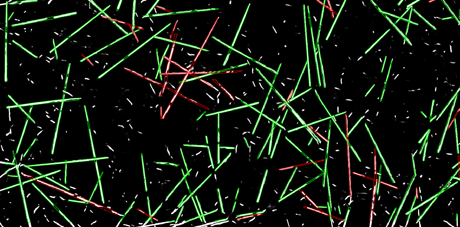
(a)

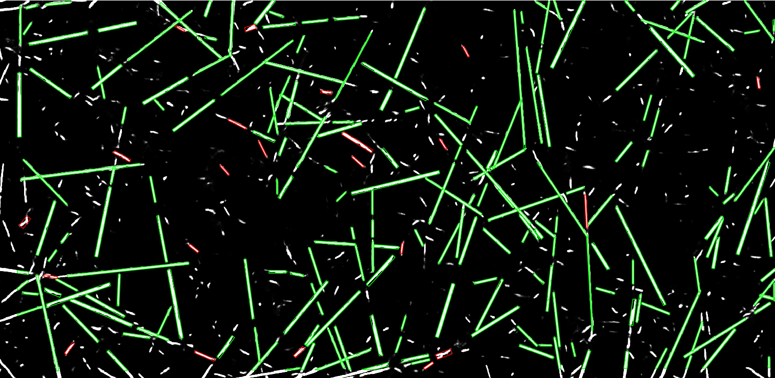
(b)

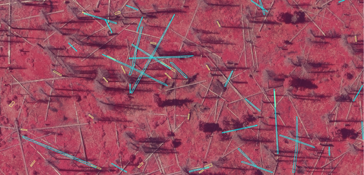
(c)

Figure 16: Results of fallen stem segmentation for plot B1 (polygon level). (a), (b) depict respectively the reference and detected polygons, with semantic segmentation posterior probability as background. Red/green colors indicate a polygon mismatched/matched with a counterpart (above 50% area overlap). (c) original false color CIR image with indicated mismatched reference (cyan) and detected (yellow) polygons.

6 Discussion

Overall, our method was successful in providing a good quality detection result for all 3 test plots of multi-level scenario complexity, both in terms of agreement of the extracted and reference polygons (IoU between 0.55-0.59), and the percentage of matched reference and detected polygons (correctness of 0.91-0.93, completeness 0.78-0.82). As expected, the shape prior turned out to be more helpful in case of polygon level evaluation, because the line level evaluation is less sensitive to changes in detected polygon width and small changes in orientation. Despite the simplicity of the utilized shape representation (rectangles parameterized by width and length), the energy benefited from an explicit shape model with a gain of up to 4 pp in completeness (while maintaining correctness). We hypothesize that a more complex shape model could show even higher gains. The test plot B1, which benefited the least from the additional energy terms, also had the lowest percentage of complex (intersecting) reference stems, confirming the intuition that the shape and collinearity priors are mostly useful for the complex scenarios.

It is interesting to note that plot B1, which can be considered the ’easiest’, obtained the lowest precision score among the 3 test plots on the polygon level. This can be attributed to a relatively high number of standing dead tree stems within this plot (see Fig. 16c). These stems appear to be virtually indistinguishable from lying stems under the semantic segmentation output of the U-Net. This is probably a consequence of the network not being trained to distinguish standing dead trees from fallen stems. It is not clear whether this can be achieved solely based on monocular images without dense depth information. Aside from standing dead trees, other sources of false negatives may be linked to root plates as well as woody debris appearing to possess a similar hue within the CIR images as our target objects.

A number of misdetections (unmatched reference trees) is once again associated with the posterior probability of the semantic segmentation from the U-Net. As visible on Figs. 16a, 17a, 18a, the missing stems are often fragmented into discontinuous chunks in the probability image, caused mostly by shadows and occlusions from other objects like shrubs or understory growth. Such discontinuities prohibit the energy function from enclosing the disjoint stem parts in a single detected polygon. This is associated with our method’s inherent tendency to exploit the connectivity structure of the high-probability pixels, where each connected component is processed independently. Due to computational tractability considerations, for large scenes it is impractical to consider all connected components within one, simultaneous optimization problem. However, there are several alternative possibilities of alleviating this problem. First, explicitly adding examples of shadowed fallen stems to the U-Net’s training set would help increase the continuity of the stems within the probability image. Second, out energy formulation could be altered to explicitly account for these discontinuous, collinear detections. Finally, a post-processing step could be applied, where the detected polygons would be clustered together based on mutual distance and collinearity, for example using graph cut methods (Shi and Malik, 2000). In our setting, the collinearity potential from Sec. 4.4.3 could be directly used in the role of the object similarity function.

Comparison to the sample consensus baseline shows that the line-based detection can be improved by applying our energy function to the SAC candidates, both in terms of completeness and correctness. Moreover, our method yields higher gains for more complex scenarios of intersecting stems. In case of simple, single-component stems, sample consensus line fitting usually delivers good results and is difficult to significantly improve upon. Also, it appears that SAC is often able to provide low-coverage partial matching of the majority of stems present within the test area, but falls short of the task of precisely delineating their extents. It is for higher stem length coverages that our multiple active contour method, endowed with prior knowledge about the size and spatial conformation of fallen stems, is able to gain the most clear advantage.

Our results show the importance of using a high-quality semantic segmentation method as a basis for the contour evolution. We believe that the performance degradation turned out to be so extreme because of the nature of the classified objects. Indeed the fallen stems are usually represented by objects of only a few pixels of width, and therefore the deformations caused by the lower-quality logistic regression semantic segmentation turned out to distort the appearance of stems in the probability image beyond recognition. It was nevertheless surprising that a ca. 20% drop in pixel-level accuracy resulted in a nearly 60% degradation in object-level recall.

The relative execution times are consistent with our a priori ordering of the three test areas with respect to their difficulty. Indeed, the unit time required for processing one stem in Plots B2 and B3 is respectively 33 % and 50 % larger compared to Plot B1 (see Table 2). The processing time is dominated by solving the multiple active contour evolution objective (via simulated annealing), with the semantic segmentation with the U-net as well as the sample consensus-based line segmentation contributing only a small fraction of time. In turn, the simulated annealing algorithm’s computational complexity can be traced back to the complexity of the move-making procedure, which is directly proportional to the number evolving model shapes as well as the number of points forming the connected component’s polygon (see Sec. 4.4). Therefore, a single connected component with a very complex boundary (e.g. Fig. 12) can dominate the the processing time, especially if the initial sample consensus line segmentation results in many model shapes to evolve. The current processing times on a single machine are satisfactory for small and medium-scale applications of areas which are densely covered with fallen stems. However, in this study our primary focus was to attain high accuracy of the stem delineation and not as much to optimize the throughput of the computation. In particular, we did not conduct investigations into the minimal required random restarts of the simulated annealing runs, the number of iterations of each temperature, or the cooling schedule itself. We believe that there is potential to reduce the current execution times by at least tenfold once these meta-parameters are optimized. This would bring the unit cost of processing a single stem into the realm of several seconds, which would mean that an area containing 10,000 fallen stems could be processed within one day on a single machine.

We believe that our study showed the advantage of using active contour evolution over generic line detection methods for the purpose of segmenting elongated structures such as fallen tree stems in high-resolution aerial imagery. To the best of our knowledge, it is the first study which (i) was based on more than 700 objects, (ii) provided both pixel-level as well as line-level detection metrics, and (iii) dealt with extremely complex overlapping stem scenes. The results show that a segmentation method which is informed on the shape and appearance of the objects it is trying to segment can improve performance especially in the case of complex scenes. A further advantage of our proposed method over off-the-shelf segmentation procedures is that most of the crucial parameters can be learned from training examples. However, it should be noted that our study had several limitations that should be addressed in future research. First, the presence of shadows and occlusions can be detrimental to the formation of connected components within the posterior probability image, leading to partition of the same physical object into multiple, unrelated segmented objects. Moreover, the utilized rectangular representation of stems may be too simple in some cases, especially in the context of applying the method to more complex shapes aside from fallen stems. Also, our input data lacked 3D information, which led to confusion between fallen and standing trees in some cases. Finally, the meta-parameters of the simulated annealing optimizer were not tuned for efficiency of processing, which makes the current version of our software not applicable to large area processing. Nonetheless, we believe that the trainable nature of the key parameters makes our approach applicable to new, previously unseen areas given enough training data, without the need for manual parameter tweaking.

Our results are very promising as we can count the number of fallen trees and determine the area covered by each tree very accurately from aerial imagery. Therefore, the proposed methodology will allow many applications in forest and conservation management. After severe disturbances, our method allows a quick assessment of the number and distribution of fallen trees, which is necessary to plan salvage logging activities to harvest the timber and to prevent the spread of insects, such as the Norway spruce bark beetle Ips typographus. In the next step, the delineated polygons will be a basis for determining not only the number of the fallen trees, but also the amount of wood. This would make the information even more suitable for forest management, since from this value the operation of logging machinery and transportation can be planned accurately. For conservation management, our method will help to map the distribution and amount of deadwood in the ecosystem. This will allow to determine the best areas for conservation measures and to monitor the amount of lying dead wood in a given area to fulfil minimum requirements for maintaining biodiversity (Müller and Bütler, 2010). Moreover, our method can also be used for research projects that need accurate information about the distribution of lying dead wood, such as long-term studies on carbon sequestration, the spatial arrangement of forest regeneration, or animal movement.

7 Conclusions and outlook

This work introduced a framework for segmenting multiple objects of a common type from imagery using a collection of evolving active contours, unified under an aggregate energy functional encompassing various aspects of the segmentation quality. In particular, along with the usual data fit term, our energy favors high-probability shapes as defined by an explicit shape model, and penalizes overlap of adjacent contours. The proposed approach makes use of state-of-the-art semantic segmentation methods (e.g. U-net) to extract regions of the input image which are likely to contain realizations of target class objects. We then instantiated the framework in the context of fallen tree detection from high-resolution aerial color infrared imagery, by providing concrete shape parametrizations, a kernel density estimator-based shape model, as well as additional, domain-specific energy potentials. It was shown on 3 test plots that our approach can achieve good segmentation performance in terms of both polygon-based (intersection-over-union) and line-based quality metrics. It was found that using the proposed shape model improved the segmentation completeness at polygon level by up to 4 pp. As expected, the additional energy terms (collinearity and shape model) were mostly useful for complex aggregates of multiple overlapping stems, while their impact on isolated stem detection was minimal.

Our investigation showed the critical importance of using a high-quality semantic segmentation method in case of thin, elongated objects such as fallen stems. The posterior probability map obtained from a simple baseline using channel intensities resulted in a breakdown of segmentation completeness, with many stems under-represented and fragmented in the probability image. The sufficient quality of the semantic segmentation is a precondition for the successful application of our method.

On the line level, the proposed energy-based segmentation method was compared to a sample consensus baseline. Although the energy functional evolves polygons (contours), an improvement in line-based metrics was also observed, with gains in both precision and recall up to 6 pp.

An issue to be addressed in future work is associated with objects split by shadows or occlusions in the probability image, leading to fragmentations of stems into disjoint parts. For large scenes with hundreds or thousands of objects, it would be computationally intractable to jointly consider all high-probability image regions within one optimization problem. Instead, a more feasible strategy seems to perform merging of the detected polygons as a post-processing step, e.g. using a graph-cut approach. Another natural direction for future work is the application of our framework to more complex object classes and associated, richer shape models. Also, instantiating the framework in 3D using outputs from voxel-based deep semantic segmentation networks could be an interesting next step.

References

- Akeret et al. (2017) Akeret, J., Chang, C., Lucchi, A., Refregier, A., 2017. Radio frequency interference mitigation using deep convolutional neural networks. Astronomy and Computing 18, 35–39.
- Arnab and Torr (2017) Arnab, A., Torr, P.H.S., 2017. Pixelwise instance segmentation with a dynamically instantiated network. CoRR abs/1704.02386. URL: http://arxiv.org/abs/1704.02386.
- Cremers and Rousson (2007) Cremers, D., Rousson, M., 2007. Efficient kernel density estimation of shape and intensity priors for level set segmentation, in: Deformable Models. Springer, New York. Topics in Biomedical Engineering. International Book Series, pp. 447–460. URL: http://dx.doi.org/10.1007/978-0-387-68343-0_13, doi:10.1007/978-0-387-68343-0_13.
- Cremers et al. (2007) Cremers, D., Rousson, M., Deriche, R., 2007. A review of statistical approaches to level set segmentation: Integrating color, texture, motion and shape. Int. J. Comput. Vision 72, 195–215. URL: http://dx.doi.org/10.1007/s11263-006-8711-1, doi:10.1007/s11263-006-8711-1.
- Dong et al. (2017) Dong, H., Yang, G., Liu, F., Mo, Y., Guo, Y., 2017. Automatic brain tumor detection and segmentation using u-net based fully convolutional networks, in: Valdés Hernández, M., González-Castro, V. (Eds.), Medical Image Understanding and Analysis, Springer International Publishing, Cham. pp. 506–517.
- Douglas and Peucker (1973) Douglas, D.H., Peucker, T.K., 1973. Algorithms for the reduction of the number of points required to represent a digitized line or its caricature. Cartographica: The International Journal for Geographic Information and Geovisualization 10, 112–122. URL: https://doi.org/10.3138/FM57-6770-U75U-7727, doi:10.3138/FM57-6770-U75U-7727.
- Duan et al. (2017) Duan, F., Wan, Y., Deng, L., 2017. A novel approach for coarse-to-fine windthrown tree extraction based on unmanned aerial vehicle images. Remote Sensing 9. URL: https://www.mdpi.com/2072-4292/9/4/306, doi:10.3390/rs9040306.
- Einzmann et al. (2017) Einzmann, K., Immitzer, M., Böck, S., Bauer, O., Schmitt, A., Atzberger, C., 2017. Windthrow detection in european forests with very high-resolution optical data. Forests 8. URL: https://www.mdpi.com/1999-4907/8/1/21, doi:10.3390/f8010021.
- Fischler and Bolles (1981) Fischler, M.A., Bolles, R.C., 1981. Random sample consensus: A paradigm for model fitting with applications to image analysis and automated cartography. Commun. ACM 24, 381–395. URL: https://doi.org/10.1145/358669.358692, doi:10.1145/358669.358692.
- Freeman et al. (2016) Freeman, M., Stow, D., Roberts, D., 2016. Object-based image mapping of conifer tree mortality in san diego county based on multitemporal aerial ortho-imagery. Photogrammetric Engineering & Remote Sensing 82, 571–580. doi:10.14358/PERS.82.7.571.
- He et al. (2017) He, K., Gkioxari, G., Dollar, P., Girshick, R., 2017. Mask r-cnn, in: 2017 IEEE International Conference on Computer Vision (ICCV), pp. 2980–2988.
- Jensen (2006) Jensen, J.R., 2006. Remote Sensing of the Environment: An Earth Resource Perspective (2nd Edition). Prentice Hall, Upper Saddle River. URL: http://www.worldcat.org/isbn/0131889508.
- Kingma and Ba (2017) Kingma, D.P., Ba, J., 2017. Adam: A method for stochastic optimization. arXiv:1412.6980.
- Kirkpatrick et al. (1983) Kirkpatrick, S., Gelatt, C.D., Vecchi, M.P., 1983. Optimization by simulated annealing. Science 220 4598, 671--80.
- Latifi et al. (2018) Latifi, H., Dahms, T., Beudert, B., Heurich, M., Kübert, C., Dech, S., 2018. Synthetic rapideye data used for the detection of area-based spruce tree mortality induced by bark beetles. GIScience & Remote Sensing 55, 839--859. URL: https://doi.org/10.1080/15481603.2018.1458463, doi:10.1080/15481603.2018.1458463.
- Lausch et al. (2013) Lausch, A., Heurich, M., Fahse, L., 2013. Spatio-temporal infestation patterns of Ips typographus (L.) in the Bavarian Forest National Park, Germany. Ecological Indicators 31, 73--81.
- Leica (2017) Leica, 2017. Leica Geosystems DMC III Airborne Digital Camera product sheet. https://leica-geosystems.com/products/airborne-systems/imaging-sensors/leica-dmciii. Accessed: 2021-02-04.
- Li and Scheraga (1987) Li, Z., Scheraga, H.A., 1987. Monte carlo-minimization approach to the multiple-minima problem in protein folding. Proceedings of the National Academy of Sciences 84, 6611--6615. URL: https://www.pnas.org/content/84/19/6611, doi:10.1073/pnas.84.19.6611, arXiv:https://www.pnas.org/content/84/19/6611.full.pdf.
- Long et al. (2015) Long, J., Shelhamer, E., Darrell, T., 2015. Fully convolutional networks for semantic segmentation. arXiv:1411.4038.
- Lopes Queiroz et al. (2019) Lopes Queiroz, G., McDermid, G.J., Castilla, G., Linke, J., Rahman, M.M., 2019. Mapping coarse woody debris with random forest classification of centimetric aerial imagery. Forests 10. URL: https://www.mdpi.com/1999-4907/10/6/471, doi:10.3390/f10060471.
- Lorensen and Cline (1987) Lorensen, W.E., Cline, H.E., 1987. Marching cubes: A high resolution 3d surface construction algorithm, in: Proceedings of the 14th Annual Conference on Computer Graphics and Interactive Techniques, Association for Computing Machinery, New York, NY, USA. pp. 163--169. URL: https://doi.org/10.1145/37401.37422, doi:10.1145/37401.37422.
- Marchi et al. (2018) Marchi, N., Pirotti, F., Lingua, E., 2018. Airborne and terrestrial laser scanning data for the assessment of standing and lying deadwood: Current situation and new perspectives. Remote Sensing 10. URL: https://www.mdpi.com/2072-4292/10/9/1356, doi:10.3390/rs10091356.
- Marcos et al. (2018) Marcos, D., Tuia, D., Kellenberger, B., Zhang, L., Bai, M., Liao, R., Urtasun, R., 2018. Learning deep structured active contours end-to-end, in: The IEEE Conference on Computer Vision and Pattern Recognition (CVPR).
- Maturana and Scherer (2015) Maturana, D., Scherer, S., 2015. Voxnet: A 3d convolutional neural network for real-time object recognition, in: 2015 IEEE/RSJ International Conference on Intelligent Robots and Systems (IROS), pp. 922--928.
- Milan et al. (2014) Milan, A., Roth, S., Schindler, K., 2014. Continuous energy minimization for multitarget tracking. IEEE Transactions on Pattern Analysis and Machine Intelligence 36, 58--72.
- Müller and Bütler (2010) Müller, J., Bütler, R., 2010. A review of habitat thresholds for dead wood: a baseline for management recommendations in european forests. European Journal of Forest Research 129, 981--992.
- Nievergelt and Preparata (1982) Nievergelt, J., Preparata, F.P., 1982. Plane-sweep algorithms for intersecting geometric figures. Commun. ACM 25, 739--747. URL: https://doi.org/10.1145/358656.358681, doi:10.1145/358656.358681.
- Ostovar et al. (2019) Ostovar, A., Talbot, B., Puliti, S., Astrup, R., Ringdahl, O., 2019. Detection and classification of root and butt-rot (rbr) in stumps of norway spruce using rgb images and machine learning. Sensors 19. URL: https://www.mdpi.com/1424-8220/19/7/1579, doi:10.3390/s19071579.
- Panagiotidis et al. (2019) Panagiotidis, D., Abdollahnejad, A., Surovy, P., Kuželka, K., 2019. Detection of fallen logs from high-resolution uav images. New Zealand Journal of Forestry 49. doi:10.33494/nzjfs492019x26x.
- Polewski et al. (2020) Polewski, P., Shelton, J., Yao, W., Heurich, M., 2020. Segmentation of single standing dead trees in high-resolution aerial imagery with generative adversarial network-based shape priors. ISPRS - International Archives of the Photogrammetry, Remote Sensing and Spatial Information Sciences XLIII-B2-2020, 717--723. URL: https://www.int-arch-photogramm-remote-sens-spatial-inf-sci.net/XLIII-B2-2020/717/2020/, doi:10.5194/isprs-archives-XLIII-B2-2020-717-2020.
- Polewski et al. (2015a) Polewski, P., Yao, W., Heurich, M., Krzystek, P., Stilla, U., 2015a. Detection of fallen trees in ALS point clouds using a Normalized Cut approach trained by simulation. ISPRS Journal of Photogrammetry and Remote Sensing 105, 252 -- 271. doi:http://dx.doi.org/10.1016/j.isprsjprs.2015.01.010.
- Polewski et al. (2015b) Polewski, P., Yao, W., Heurich, M., Krzystek, P., Stilla, U., 2015b. Detection of single standing dead trees from aerial color infrared imagery by segmentation with shape and intensity priors. ISPRS Annals of Photogrammetry, Remote Sensing and Spatial Information Sciences II-3/W4, 181--188. doi:10.5194/isprsannals-II-3-W4-181-2015.
- Polewski et al. (2017) Polewski, P., Yao, W., Heurich, M., Krzystek, P., Stilla, U., 2017. A voting-based statistical cylinder detection framework applied to fallen tree mapping in terrestrial laser scanning point clouds. ISPRS Journal of Photogrammetry and Remote Sensing 129, 118 -- 130. doi:http://dx.doi.org/10.1016/j.isprsjprs.2017.04.023.
- Ren et al. (2017) Ren, S., He, K., Girshick, R., Sun, J., 2017. Faster r-cnn: Towards real-time object detection with region proposal networks. IEEE Transactions on Pattern Analysis and Machine Intelligence 39, 1137--1149.
- Ronneberger et al. (2015) Ronneberger, O., P.Fischer, Brox, T., 2015. U-net: Convolutional networks for biomedical image segmentation, in: Medical Image Computing and Computer-Assisted Intervention (MICCAI), Springer. pp. 234--241. URL: http://lmb.informatik.uni-freiburg.de/Publications/2015/RFB15a. (available on arXiv:1505.04597 [cs.CV]).
- Russakovsky et al. (2015) Russakovsky, O., Deng, J., Su, H., Krause, J., Satheesh, S., Ma, S., Huang, Z., Karpathy, A., Khosla, A., Bernstein, M., Berg, A.C., Fei-Fei, L., 2015. ImageNet Large Scale Visual Recognition Challenge. International Journal of Computer Vision (IJCV) 115, 211--252. doi:10.1007/s11263-015-0816-y.
- Safonova et al. (2019) Safonova, A., Tabik, S., Alcaraz-Segura, D., Rubtsov, A., Maglinets, Y., Herrera, F., 2019. Detection of fir trees (abies sibirica) damaged by the bark beetle in unmanned aerial vehicle images with deep learning. Remote Sensing 11. URL: https://www.mdpi.com/2072-4292/11/6/643, doi:10.3390/rs11060643.
- Seibold and Thorn (2018) Seibold, S., Thorn, S., 2018. The Importance of Dead-Wood Amount for Saproxylic Insects and How It Interacts with Dead-Wood Diversity and Other Habitat Factors. Springer International Publishing, Cham. pp. 607--637. URL: https://doi.org/10.1007/978-3-319-75937-1_18, doi:10.1007/978-3-319-75937-1_18.
- Seidl et al. (2017) Seidl, R., Thom, D., Kautz, M., Martin-Benito, D., Peltoniemi, M., Vacchiano, G., Wild, J., Ascoli, D., Petr, M., Honkaniemi, J., Lexer, M.J., Trotsiuk, V., Mairota, P., Svoboda, M., Fabrika, M., Nagel, T.A., Reyer, C.P.O., 2017. Forest disturbances under climate change. Nature Climate Change 7, 395--402. URL: https://doi.org/10.1038/nclimate3303, doi:10.1038/nclimate3303.
- Shi and Malik (2000) Shi, J., Malik, J., 2000. Normalized cuts and image segmentation. IEEE T. Pattern Anal. 22, 888--905. doi:10.1109/34.868688, arXiv:0703101v1.
- Siarry and Berthiau (1997) Siarry, P., Berthiau, G., 1997. Fitting of tabu search to optimize functions of continuous variables. International Journal for Numerical Methods in Engineering 40, 2449 -- 2457. doi:10.1002/(SICI)1097-0207(19970715)40:13<2449::AID-NME172>3.0.CO;2-O.
- Thiel et al. (2020) Thiel, C., Mueller, M.M., Epple, L., Thau, C., Hese, S., Voltersen, M., Henkel, A., 2020. Uas imagery-based mapping of coarse wood debris in a natural deciduous forest in central germany (hainich national park). Remote Sensing 12. URL: https://www.mdpi.com/2072-4292/12/20/3293, doi:10.3390/rs12203293.
- Tucker (1979) Tucker, C.J., 1979. Red and photographic infrared linear combinations for monitoring vegetation. Remote Sens. Environ. 8, 127--150. doi:10.1016/0034-4257(79)90013-0.
- Wales and Doye (1997) Wales, D.J., Doye, J.P.K., 1997. Global optimization by basin-hopping and the lowest energy structures of lennard-jones clusters containing up to 110 atoms. The Journal of Physical Chemistry A 101, 5111--5116. URL: https://doi.org/10.1021/jp970984n, doi:10.1021/jp970984n.
- Wand and Jones (1994) Wand, M.P., Jones, C., 1994. Multivariate plug-in bandwidth selection. Computational Statistics 9, 97--116.
- Watson et al. (2018) Watson, J.E.M., Evans, T., Venter, O., Williams, B., Tulloch, A., Stewart, C., Thompson, I., Ray, J.C., Murray, K., Salazar, A., McAlpine, C., Potapov, P., Walston, J., Robinson, J.G., Painter, M., Wilkie, D., Filardi, C., Laurance, W.F., Houghton, R.A., Maxwell, S., Grantham, H., Samper, C., Wang, S., Laestadius, L., Runting, R.K., Silva-Chávez, G.A., Ervin, J., Lindenmayer, D., 2018. The exceptional value of intact forest ecosystems. Nature Ecology & Evolution 2, 599--610. doi:10.1038/s41559-018-0490-x.
- Žalik (2000) Žalik, B., 2000. Two efficient algorithms for determining intersection points between simple polygons. Computers & Geosciences 26, 137 -- 151. URL: http://www.sciencedirect.com/science/article/pii/S0098300499000710, doi:https://doi.org/10.1016/S0098-3004(99)00071-0.
- Zhao et al. (2018) Zhao, Z., Zheng, P., Xu, S., Wu, X., 2018. Object detection with deep learning: A review. CoRR abs/1807.05511. URL: http://arxiv.org/abs/1807.05511, arXiv:1807.05511.