^b Korea Institute for Advanced Study
Seoul, 02455,  Korea
e-mail: mukhanov@physik.lmu.de

^d National Research Nuclear University MEPhI
(Moscow Engineering Physics Institute),
Kashirskoe Shosse 31, 115409 Moscow, Russia

^e Dubna State University,
141980 Dubna (Moscow region), Russia

Abstract

We consider new instantons that appear as a result of accounting for quantum fluctuations. These fluctuations naturally regularize the $O(4)$ singular solutions abandoned in Coleman’s theory. In the previous works [4, 3] we showed how new instantons modify the widely accepted picture of false vacuum decay in two particular examples of exactly solvable potentials. Here we generalize our consideration to arbitrary potentials and provide a general theory of these new instantons with quantum cores in which vacuum fluctuations dominate. We develop a method that allows us to determine the parameters of instantons for generic potentials not only in the thin-wall approximation but also in the cases where this approximation fails. Unlike the Coleman instantons, the instantons with quantum cores always exist in the cases where the vacuum must be unstable.

1 Introduction

Let us consider a real scalar field with the potential $V\left(\varphi\right)$ shown in Fig.1. For simplicity, we normalize this potential to zero at the local minimum at $\varphi_{f}<0$, i.e., $V\left(\varphi_{f}\right)=0$. The potential has a maximum at $\varphi=0$, where $V\text{$\left(0\right)$}=V_{bar}$ is the hight of the barrier. If at $\varphi>0$ the potential is unbounded from below or negative at the second minimum, which corresponds to the true vacuum, then the false vacuum at $\varphi_{f}$ is obviously metastable and must decay. As a result of the sub-barrier tunneling, the critical bubbles are formed, which are filled with a new phase $\varphi>0$. They expand and eventually collide, filling the space with a new phase.

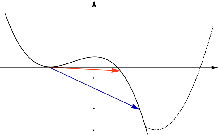
$\varphi_{f}$

$V$

$\varphi$

$-V_{bar}$

$V_{uv}$

$V_{true}$

$V_{bar}$

Figure 1: The potential with a metastable vacuum at $\varphi_{f}$, which must decay via instantons, regardless of whether this potential is unbounded from below or has the second true minimum (represented by the dot-dashed line). For each concrete potential, there is a full spectrum of instantons. Those instantons corresponding to the transitions represented by the upper red line describe the thin-wall bubbles for which the potential in the center of the emerging bubble satisfies the condition $\left|V_{uv}\right|\ll V_{bar}$. The instantons corresponding to the deep subbarrier transition (as shown, for example, by the lower blue line) are dominated by “friction” and cannot be described in the thin-wall approximation.

At first sight, the problem looks very similar to the problem of tunneling the “particle” with $N$ degrees of freedom, characterized by generalized coordinates $\mathbf{q\mathnormal{\equiv(}}q_{1},...,q_{N})$, from the local minimum of the potential $V\left(\mathbf{q}\right)$. However, this analogy is incomplete and, moreover, even confusing. In fact, for a system with a finite number degrees of freedom, the subbarrier transition is reversible, i.e., the system can return to the original minimum after tunneling. In field theory, vacuum decay is irreversible. Although there are solutions that seem to describe a transition that takes us back to a false vacuum state, they correspond to contracting bubbles with very improbable initial conditions of zero measure. Moreover, we would like to emphasize that the scalar field potential $V\left(\varphi\right)$ should in no way be considered as an analogue of the potential $V\left(\mathbf{q}\right)$. To make this clear, it is convenient to represent the action for the scalar field

$$S=\int\left(\frac{1}{2}\eta^{\alpha\beta}\varphi_{,\alpha}\varphi_{,\beta}-V\left(\varphi\right)\right)d^{4}x\,,$$ (1)

where $\eta^{\alpha\beta}$ is the Minkowski metric, in the following equivalent form:

$$S=\int(\mathcal{K-V)}dt\,,$$ (2)

where

$$\mathcal{K}\equiv\frac{1}{2}\int\left(\partial_{t}\varphi_{\mathbf{x}}\right)d^{3}x\,,$$ (3)

and

$$\mathcal{V}\equiv\int\left(\frac{1}{2}\left(\partial_{i}\varphi_{\mathbf{x}}\right)^{2}+V\left(\varphi_{\mathbf{x}}\right)\right)d^{3}x\,.$$ (4)

From here it is obvious that we consider a system with an infinite number of degrees of freedom, described by generalized coordinates $\varphi_{\mathbf{x}}(t)\equiv\varphi\left(\mathbf{x\mathnormal{,t}}\right)$, which characterizes the strength of the field at each point in space, and the spatial coordinates $\mathbf{x=}\left(x^{1},x^{2},x^{3}\right)$ simply enumerate the degrees of freedom. Accordingly, $\mathcal{K}$ and $\mathcal{V}$ are the kinetic and potential energies of the system. Therefore, the functional $\mathcal{V}\left(\varphi_{\mathbf{x}}\right)$ (but not $V\left(\varphi\right)$) plays the role of the potential when we consider sub-barrier tunneling in quantum field theory. If the minimum at $\varphi_{f}$ corresponds to a false vacuum, then the potential $\mathcal{V}\left(\varphi_{\mathbf{x}}\right)$ is always unbounded from below even for the bound potential $V\left(\varphi\right)$ with the second true minimum of depth $V\left(\varphi_{tr}\right)=-\epsilon$. Indeed, in this case, the constant field configuration $\varphi=\varphi_{tr}$ has the potential energy $\mathcal{V}\left(\varphi_{\mathbf{x}}=\varphi_{tr}\right)=-\epsilon\times volume$ and tends to minus infinity as the volume grows. Therefore, the false vacuum decay is always analogous to the sub-barrier escape of the “particle with an infinite number degrees of freedom” from a local well in the unbounded potential. To describe the sub-barrier transition, it is convenient to perform the Wick rotation and switch from Minkowski to Euclidean time $\tau=\mathsf{i}\,t$. The action (2) then becomes $S=\mathsf{i}\,S_{E}$, where

$$S_{E}=\int\left(\frac{1}{2}\left(\partial_{\tau}\varphi\right)^{2}+\frac{1}{2}\left(\partial_{i}\varphi\right)^{2}+V\left(\varphi\right)\right)d^{3}xd\tau$$ (5)

is the Euclidean action. Assuming that the sub-barrier transition from the false vacuum occurs in the “time interval” $0\geq\tau>-\infty$, we must find field configurations with $\varphi\left(\tau\rightarrow-\infty,\mathbf{x}\right)=\varphi_{f}$, matching the classically allowed state $\varphi\left(\tau=0,\mathbf{x}\right)$ with $\partial\varphi/\partial\tau=0$ and $\mathcal{V}\left(\varphi\left(\mathbf{x}\right)\right)=0$. It is clear that the main contribution to the tunneling rate, proportional to $\exp\left(iS\right)=\exp\left(-S_{E}\right)$, should come from those field configurations that minimize the Euclidean action, i.e., satisfy the equation

$$\partial_{\tau}^{2}\varphi+\Delta\varphi-V^{\prime}=0\,,$$ (6)

where $V^{\prime}\equiv dV/d\varphi.$ Therefore, to calculate the tunneling rate, one must first find the corresponding solutions of equation (6).

2 The Coleman Instanton and Quantum Fluctuations

From general considerations, one can expect that among all possible solutions of equation (6), the solution with the highest possible symmetry has the smallest action and dominates the decay rate [1, 2]. Therefore, Coleman proposed to consider $O(4)$ - invariant solutions for which $\varphi$ depends only on $\varrho=\sqrt{\tau^{2}+\mathbf{x}^{2}}$, that is, $\varphi\left(\tau,\mathbf{x}\right)=\varphi\left(\varrho\right)$. In this case, equation (6) is simplified to the ordinary differential equation

$$\ddot{\varphi}(\varrho)+\frac{3}{\varrho}\,\dot{\varphi}(\varrho)-V^{\prime}=0\,,$$ (7)

where the dot denotes the derivative with respect to $\varrho.$ This reduces the problem to studying “the motion of a particle with one degree of freedom” in the presence of friction in the inverted potential $V$ (see Fig.2) .

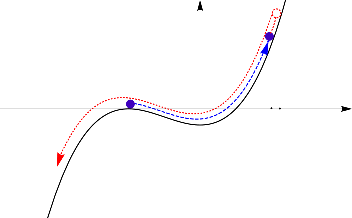
$\varphi_{f}$

$-V$

$\varphi$

$\varphi_{uv}$

$\varphi_{b}$

$\varrho_{b}\neq 0$

$\varrho_{uv}$

$\varrho\rightarrow\infty$

$\varrho\rightarrow 0$

Figure 2: The solution of equation (7) for the instanton is mathematically equivalent to the solution of the equation for the “particle” with friction in the inverted potential $-V$. It starts its motion at $\varrho\rightarrow\infty$ on the top of the inverted potential and moves toward positive $\varphi$ when the “time” $\varrho$ decreases, as shown by the dashed blue line. At some $\varrho_{b}\neq 0$, the “velocity” $\dot{\varphi}$ vanishes and the “particle” bounces off and starts moving in the direction of negative $\varphi$, as shown by the dotted red line. Only when $\varrho_{b}=0$, the motion ends at the highest point and does not go further back. This is the case of the nonsingular Coleman instanton, which at this moment materializes as a bubble in the Minkowski space. For any finite $\varrho_{b}$ the bouncing classical trajectories are singular. However, as we have shown, the classical solutions corresponding to these singular trajectories can be trusted only up to $\varrho_{uv}>\varrho_{b}$ because at this moment quantum fluctuations begin to dominate and therefore the part of the solution indicated by the dotted red line must be ignored and only the part, shown by the dashed blue line, can be trusted. At $\varrho=\varrho_{uv}$, the bubble with the quantum core of size $\varrho_{uv}$, where the potential is shifted to $V_{uv}$, emerges from under the barrier and materializes in the Minkowski space.

In order to find a particular solution of (7) that makes a dominant contribution to the tunneling rate, we need to decide what are the proper initial or, alternatively, boundary conditions for this solution. One of them is obvious: namely, if the field is “initially” in the false vacuum state at $\tau\rightarrow-\infty$, then

$$\varphi\left(\varrho\rightarrow\infty\right)=\varphi_{f}\,.$$ (8)

Assuming that at the “moment of emergence” at $\tau=0$ the field in the center of the bubble is equal to $\varphi\left(\varrho=0\right)=\varphi_{c}$, we can approximate (7) near this point, i.e., for $\left|\varphi-\varphi_{c}\right|\ll\varphi_{c}$, as

$$\ddot{\varphi}(\varrho)+\frac{3}{\varrho}\,\dot{\varphi}(\varrho)-V_{c}^{\prime}\simeq 0\,,$$ (9)

where $V_{c}^{\prime}=V^{\prime}\left(\varphi_{c}\right)$. This equation has the following general solution:

$$\varphi\left(\varrho\right)=\varphi_{c}+\frac{V_{c}^{\prime}}{8}\,\varrho^{2}+\frac{C}{\varrho^{2}}\,,$$ (10)

where the integration constant $C$ must be taken equal to zero in order to be in agreement with $\varphi\left(\varrho=0\right)=\varphi_{c}$. Therefore,

$$\dot{\varphi}(\varrho=0)=0$$ (11)

is the only possible choice for the boundary condition at $\varrho=0$ that does not lead to a singularity. The $O(4)$-solution of equation (7) with boundary conditions (8) and (11), if it exists, is unique and is called the Coleman instanton.

We showed in previous publications that in some cases such instantons either do not exist [3] or they lead to an unexpectedly large vacuum decay rate [4]. As we demonstrated in [3, 4], both these problems can be resolved by involving unavoidable quantum fluctuations. These fluctuations can either regularize the solutions, which were previously singular, or completely saturate the instantons leading to too large a decay rate. In fact, the classical solution can be trusted only if the field strength exceeds the level of vacuum fluctuations at the appropriate scale. In the case of a massless scalar field, the “typical” amplitude of quantum fluctuations and their time derivative in scales $r$ are approximately equal to (see, e.g., [5, 6])

$$\left|\delta\varphi_{r}\right|\simeq\frac{\sigma}{r}\,,\quad\left|\delta\dot{\varphi}_{r}\right|\simeq\frac{\sigma}{r^{2}}\,,$$ (12)

where $\sigma$ is the number of the order of unity. The massless scalar field is a shift invariant, and to determine when quantum fluctuations begin to saturate the classical field, we must compare either the typical change of this field on scales $r$ or its time derivative with the amplitude given in (12). Both equations lead to the same result (up to a numerical coefficient of the order of unity). Therefore, to be concrete, we compare the time derivative for the instanton solution $\dot{\varphi_{I}}\left(\varrho\right)$ with $\left|\delta\dot{\varphi}_{r}\right|$. It is clear that the instanton solution is trustworthy only at such $r$ for which

$$\dot{\varphi_{I}}\left(\sqrt{\tau^{2}+r^{2}}\right)>\frac{\sigma}{r^{2}}\,.$$ (13)

In Fig.3, we have plotted two solutions for the Coleman instanton versus the level of quantum fluctuations at $\tau=0$ when $r=\varrho.$ The instanton lying entirely under the $\sigma/\varrho^{2}$ curve is never reliable, while the other is reliable only in the $\varrho_{uv}<\varrho<\varrho_{ir}$ region, where both the ultraviolet and the infrared cutoff scales, $\varrho_{uv}$ and $\varrho_{ir}$, are two different solutions of the following equation:

$$\dot{\varphi}_{I}\left(\varrho\right)\simeq\frac{\sigma}{\varrho^{2}}\,.$$ (14)

$-\dot{\varphi}$

$\varrho$

$\varrho_{ir}$

$\varrho_{uv}$

$|\dot{\varphi}_{I}|$

$|\delta\dot{\varphi}_{\varrho}|\sim\frac{1}{\varrho^{2}}$

Figure 3: The red dot-dashed line indicates the level of quantum fluctuations. The classical solution with the Coleman boundary conditions, represented by the blue dot-dashed line, is completely hidden under the quantum fluctuations and is not trustworthy. For the Coleman instanton, shown by the black solid line, the reliable part of the classical solution lies in the region $\varrho_{uv}<\varrho<\varrho_{ir}$, where the strength of the field exceeds the level of the quantum fluctuations.

It follows that Coleman’s boundary condition (11) formulated in the deep ultraviolet region is never reliable. In turn, the boundary condition formulated at a small finite $\varrho_{b}\neq 0$ does not a priori exclude solutions with the non-vanishing integration constant $C$ in (10). A possible singularity that can occur in this case at $\varrho=0$ is anyway regularised by the ultraviolet cutoff. This leads to the appearance of the whole class of new instantons that can be parametrized by $\varrho_{b}$.

3 New Instantons

To determine the plausible boundary condition at $\varrho_{b}$, we first calculate the potential energy (4) at $-\varrho_{b}\leq\tau\leq 0$. For the $O\left(4\right)$-invariant solution $\varphi\left(\varrho\right)$, the integral in (4) is simplified to

$$\mathcal{V}\left(\tau\right)=4\pi\int_{\varrho_{b}}^{\infty}\left[\frac{1}{2}\left(1-\frac{\tau^{2}}{\varrho^{2}}\right)^{3/2}\dot{\varphi}^{2}+\left(1-\frac{\tau^{2}}{\varrho^{2}}\right)^{1/2}V\right]\varrho^{2}d\varrho+\mathcal{V}_{r_{b}}\left(\tau\right)\,,$$ (15)

where $\mathcal{V}_{r_{b}}\left(\tau\right)$ is the contribution to the potential energy from the core of the bubble of size $r_{b}\left(\tau\right)=\sqrt{\varrho_{b}^{2}-\tau^{2}}$. Integrating by parts and using equation of motion (7), we can rewrite the second term under the integral as

$$4\pi\int_{\varrho_{b}}^{\infty}\left(1-\frac{\tau^{2}}{\varrho^{2}}\right)^{1/2}V\varrho^{2}d\varrho=\frac{4\pi}{3}\int_{\varrho_{b}}^{\infty}Vd\left(\varrho^{2}-\tau^{2}\right)^{3/2}$$

$$=\frac{4\pi}{3}\left(\left.\left(\varrho^{2}-\tau^{2}\right)^{3/2}V\right|_{\varrho_{b}}^{\infty}-\int_{\varrho_{b}}^{\infty}\left(\varrho^{2}-\tau^{2}\right)^{3/2}\left(\ddot{\varphi}+\frac{3}{\varrho}\dot{\varphi}\right)\dot{\varphi}d\varrho\right)\,.$$ (16)

If we remove here the term with the second derivative by further integration by parts and insert the result in (15), we obtain

$$\mathcal{V}\left(\tau\right)=2\,\pi\,\tau^{2}\int_{\varrho_{b}}^{\infty}\sqrt{1-\frac{\tau^{2}}{\varrho^{2}}}\,\dot{\varphi}^{2}d\varrho+\frac{2\,\pi}{3}\,\dot{\varphi}_{b}^{2}\,r_{b}^{3}-\frac{4\,\pi}{3}\,V_{b}\,r_{b}^{3}+\mathcal{V}_{r_{b}}\left(\tau\right)\,,$$ (17)

where $\dot{\varphi}_{b}\equiv\dot{\varphi}\left(\varrho_{b}\right)$, $V_{b}\equiv V\left(\varphi\left(\varrho_{b}\right)\right)$ and we have assumed that $\dot{\varphi}^{2}\varrho^{3}$ and $V\varrho^{3}$ vanish as $\varrho\rightarrow\infty$. Since we have normalized the potential $V$ in the false vacuum to zero, the total energy of the bubble must be zero. Taking into account that $\partial_{\tau}\varphi=\frac{\tau\,\dot{\varphi}}{\sqrt{\tau^{2}+\mathbf{x}^{2}}}$, we find that the kinetic energy (3) vanishes at $\tau=0$ and therefore the bubble can materialize or, in other words, emerge from under the barrier only when

$$\mathcal{V}\left(0\right)=\frac{2\,\pi}{3}\,\dot{\varphi}_{b}^{2}\,\varrho_{b}^{3}-\frac{4\,\pi}{3}\,V_{b}\,\varrho_{b}^{3}+\mathcal{V}_{\varrho_{b}}(0)$$ (18)

vanishes. It is quite natural to assume (see the next Section for a more detailed justification), that the total energy of the central part of the bubble with the radius $r_{b}=\varrho_{b}$ is mainly due to the shift of the potential energy density $\mathcal{V}_{\varrho_{b}}(0)$ to $V_{b}$ and is therefore equal to

$$\mathcal{V}_{\varrho_{b}}(0)=\frac{4\,\pi}{3}\,V_{b}\,\varrho_{b}^{3}\,,$$ (19)

compensating the second term in (18). Since the potential energy $\mathcal{V}\left(0\right)$ must vanish, we conclude that the only possible boundary condition we can impose at $\varrho_{b}$ is

$$\dot{\varphi}\left(\varrho_{b}\right)=0\,.$$ (20)

The solutions of equation (7) with the boundary conditions (8) and (20) give us the whole class of new instantons parametrized by $\varrho_{b}$ at which the corresponding classical solution bounces.

4 Quantum Core

As can be seen in Fig.4, part of these new solutions inevitably falls below the curve determining the level of quantum fluctuations, and therefore they can be trusted only in the range $\varrho_{uv}<\varrho<\varrho_{ir}$ where $\dot{\varphi}\left(\varrho\right)$ exceeds the level of quantum fluctuations. The ultraviolet cutoff scale $\varrho_{uv}$ is always larger than $\varrho_{b}$. We will show how to determine this scale for a rather broad class of potentials. To do this, we assume that the field $\varphi$ does not change its value too much and stays close to $\varphi_{b}$ when $\varrho$ changes from $\varrho_{b}$ to $\varrho_{uv}$ . Then equation (7) can be well approximated as in (9) by replacing $\varphi_{c}$ by $\varphi_{b}$. The general solution of this equation is given in (10), where the constant of integration $C$ is now determined by the boundary condition (20). As a result, we find

$$\varphi_{I}\left(\varrho\right)=\varphi_{b}+\frac{V_{b}^{\prime}}{8}\,\frac{\left(\varrho^{2}-\varrho_{b}^{2}\right)^{2}}{\varrho^{2}}\,.$$ (21)

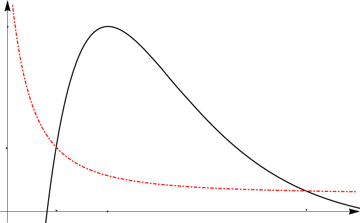
$-\dot{\varphi}$

$\varrho$

$\varrho_{ir}$

$\varrho_{m}$

$|\dot{\varphi}_{I}|$

$|\delta\dot{\varphi}_{\varrho}|\sim\frac{1}{\varrho^{2}}$

$\varrho_{uv}$

$\varrho_{b}$

$-\dot{\varphi}_{m}$

$-\dot{\varphi}_{uv}$

Figure 4: Unlike the Coleman instantons, the new instanton, shown as a solid black line, corresponds to the classical solution with the boundary condition $\dot{\varphi}\left(\varrho_{b}\right)=0$ with finite non-vanishing $\varrho_{b}$, which is a free parameter characterizing the entire spectrum of the new instantons. Being continued to $\varrho<\varrho_{b}$, this solution would become singular at $\varrho=0$ with $\varphi$ going to minus infinity. But already at $\varrho_{uv}>\varrho_{b}$ the derivative of the classical solution $|\dot{\varphi}_{I}|$ falls below the level of quantum fluctuations $|\delta\dot{\varphi}_{\varrho}|\sim\frac{1}{\varrho^{2}}$, and $\varrho_{uv}$, which is determined by the parameters characterising the classical solution, regularizes the singularity. For this reason, the part of the solution indicated by the dotted red line in Fig.2 must be ignored.

Substituting this solution into (14), we obtain the following equation:

$$\varrho_{uv}^{4}+\frac{4\,\sigma}{V_{b}^{\prime}}\,\varrho_{uv}-\varrho_{b}^{4}=0\,,$$ (22)

which can be solved exactly and gives us the ultraviolet cutoff scale in terms of $\varrho_{b}$. The equation for the infrared cutoff scale $\varrho_{ir}$ can be obtained in a similar way by considering the asymptotics of the solution at large $\varrho$. At this stage, we do not need explicit solutions for these scales but we would like to emphasize again that the bounce for a new instanton always occurs within the quantum core with the radius $\varrho_{uv}$. Quantum fluctuations dominate in this core and it makes no sense to speak about the classical solution for $\varrho<\varrho_{uv}$. Since we have normalized the energy density in the false vacuum to zero, the energy density of vacuum fluctuations in the quantum core must be shifted by $V_{uv}\equiv V(\varphi_{uv})$ ($\varphi_{uv}\equiv\varphi(\varrho_{uv})$). Taking this into account, we find the total potential energy for $\tau=0$ which comprises both the contribution of the classical instanton solution in its trustable region $\varrho_{uv}<\varrho<\varrho_{ir}$ and the energy of the quantum core:

$$\mathcal{V}\left(0\right)=\frac{2\,\pi}{3}\left(\dot{\varphi}_{uv}^{2}\,\varrho_{uv}^{3}-\dot{\varphi}_{ir}^{2}\,\varrho_{ir}^{3}\right)\simeq\frac{2\,\pi\,\sigma}{3}\left(\frac{1}{\varrho_{uv}}-\frac{1}{\varrho_{ir}}\right).$$ (23)

Thus, with the precision allowed by the time-energy uncertainty relation, the potential energy vanishes and the bubble with the quantum core emerges from under the barrier, materialises and expands in the Minkowski space, filling it with a new phase. Therefore, the after-bouncing part of the new instanton at $0<\varrho<\varrho_{b}$, which is singular at $\varrho\rightarrow 0$, must be ignored and replaced by the quantum core.

To determine the contribution of the new regularized instantons to the decay rate, we have to calculate the Euclidean action (5), which for the $O(4)$ solutions is simplified to

$$S_{E}\,=\,2\pi^{2}\,\int_{\varrho_{uv}}^{\varrho_{ir}}\left(\frac{1}{2}\,\dot{\varphi}^{2}\,+V(\varphi)\right)\varrho^{3}d\varrho+S_{QC}\,,$$ (24)

where

$$S_{QC}=\frac{\pi^{2}}{2}V_{uv}\varrho_{uv}^{4}\,$$ (25)

is the contribution from the quantum core. Using equation of motion (7) and integrating by parts, we find

$$2\pi^{2}\int_{\varrho_{uv}}^{\varrho_{ir}}V\varrho^{3}d\varrho=\frac{\pi^{2}}{2}\left(\left.V\varrho^{4}\right|_{\varrho_{uv}}^{\varrho_{ir}}-\int_{\varrho_{uv}}^{\varrho_{ir}}V^{\prime}\dot{\varphi}\varrho^{4}d\varrho\right)$$

$$=\frac{\pi^{2}}{2}\left(\left.V\varrho^{4}\right|_{\varrho_{uv}}^{\varrho_{ir}}-\int_{\varrho_{uv}}^{\varrho_{ir}}\left(\ddot{\varphi}+\frac{3}{\varrho}\dot{\varphi}\right)\dot{\varphi}\varrho^{4}d\varrho\right)$$

$$=\frac{\pi^{2}}{2}\left(\left.\left(V-\frac{1}{2}\dot{\varphi}^{2}\right)\varrho^{4}\right|_{\varrho_{uv}}^{\varrho_{ir}}-\int_{\varrho_{uv}}^{\varrho_{ir}}\dot{\varphi}^{2}\varrho^{3}d\varrho\right)\,,$$ (26)

and therefore total action (24) can be rewritten as

$$S_{E}=\frac{\pi^{2}}{2}\int_{\varrho_{uv}}^{\varrho_{ir}}\dot{\varphi}^{2}\varrho^{3}d\varrho+\frac{\pi^{2}}{4}\left(2V_{ir}\varrho_{ir}^{4}+\dot{\varphi}_{uv}^{2}\varrho_{uv}^{4}-\dot{\varphi}_{ir}^{2}\varrho_{ir}^{4}\right)\,.$$ (27)

The last term in the parentheses is of the order of unity and can be neglected because the semiclassical approximation is valid only when $S_{E}\gg 1$. Moreover,

$$\int_{\varrho_{b}}^{\varrho_{uv}}\dot{\varphi}^{2}\varrho^{3}d\varrho<\dot{\varphi}_{uv}^{2}\,\varrho_{uv}^{4}\simeq O(1)\,,$$ (28)

and the integral from $\varrho_{ir}$ to $\infty$ is also of the order of unity. Therefore, the action for the new quantum-core instantons is well approximated by

$$S_{E}=\frac{\pi^{2}}{2}\int_{\varrho_{b}}^{\infty}\dot{\varphi}^{2}\varrho^{3}d\varrho\,.$$ (29)

The decay rate of the false vacuum per unit time per unit volume can then be estimated as

$$\Gamma\simeq\varrho_{0}^{-4}\exp\left(-S_{E}\right)\,,$$ (30)

where $\varrho_{0}\equiv\varrho_{0}\left(\varrho_{b},\varphi_{f},...\right)$ is the parameter characterizing the “size of the bubble” and should enter here for dimensionality reasons.

5 General Solutions

In this section, we will find approximate instanton solutions for a broad class of unbounded potentials with a false vacuum, as shown in Fig.1 . The false vacuum at $\varphi_{f}<0$ is separated from the unbounded concave part of the potential by the barrier of hight $V_{bar}$, and at $\varphi>0$ both the first and second derivatives of the potential are negative, i.e. $V^{\prime}<0$ and $V^{\prime\prime}<0$. The typical behavior of the magnitude of the first derivative $\left|V^{\prime}\left(\varphi\right)\right|$ for the potential in Fig.1 is shown in Fig.5. It first grows, reaches its maximum $V^{\prime}_{i}$ at the inflection point located within the range $\varphi_{f}<\varphi_{i}<0$, vanishes at $\varphi=0$ and then starts to grow rapidly. We assume that the potential up to $\varphi_{i}$ can be well approximated as

$$V\left(\varphi\right)=\frac{1}{2}V_{f}^{\prime\prime}\left(\varphi-\varphi_{f}\right)^{2}+\frac{1}{4!}V_{f}^{(IV)}\left(\varphi-\varphi_{f}\right)^{4}+...\,,$$ (31)

where $V^{\prime\prime}_{f}$ and $V_{f}^{(IV)}$ are the second and fourth derivatives of the potential at $\varphi_{f}$, in particular, for the quartic potential $V^{\prime\prime}_{f}=0$. Our task is to find an approximate solution of equation (7) for a rather generic potential, simplifying this equation by neglecting either the friction or the potential term in it.

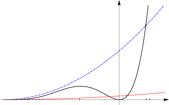
$|V^{\prime}|$

$\varphi$

$\varphi_{uv}$

$\varphi_{m}$

$\varphi_{f}$

end of friction domination

thin-wall approximation

$\varphi_{i}$

Figure 5: The magnitude of the derivative of the potential is compared to the value of the friction term in equation (7) calculated under the assumption that this term dominates. In the case shown by the blue dot-dashed line, the friction dominates over the potential term in the range $\varphi_{f}<\varphi<\varphi_{m}$, where the derivative $\left|\dot{\varphi}\right|$ grows as $\varrho$ changes from $\infty$ to $\varrho_{m}$ (see Fig.4). At $\varrho\simeq\varrho_{m}$ the potential term in (7) takes over and $\left|\dot{\varphi}\right|$ starts to decrease until finally the ultraviolet cutoff is reached. Such instantons are mostly dominated by friction and correspond to thick-wall bubbles. If, on the other hand, the friction term is almost completely below $\left|V^{\prime}\right|$, as indicated by the dashed red line, it can be neglected in the leading order and we can use the thin-wall approximation.

5.1 Friction dominated solutions (outside of the thin-wall approximation)

Given a solution of equation (7), we want to determine in what range of $\varphi$ the potential term in this equation can be neglected with respect to the friction term, i.e.,

$$\left|V^{\prime}\right|\ll\left|\frac{3}{\varrho}\dot{\varphi}\right|\,.$$ (32)

To do this, we first find the following solution of equation (7) by omitting the potential term in it and taking into account the boundary condition (8):

$$\varphi\left(\varrho\right)\simeq\varphi_{f}-\frac{E}{4\,\varphi_{f}\,\varrho^{2}}\,,$$ (33)

where $E>0$ is the integration constant, normalized to negative $4\varphi_{f}$ for convenience because as we will see, $E$ is nothing more than the number of quanta on the scale characterizing the size of the bubble. If we calculate the derivative of $\varphi$ and express $\varrho$ in terms of $\varphi$ from (33), we get

$$\left|\frac{3}{\varrho}\dot{\varphi}\right|\simeq\frac{24\left|\varphi_{f}\right|}{E}\left(\varphi_{f}-\varphi\right)^{2}\,.$$ (34)

It is clear that inequality (32) is satisfied in the region where $\left|V^{\prime}\left(\varphi\right)\right|$ lies well below the quadraric curve in (34), (see Fig. 5). Therefore, for

$$E\ll\frac{24\left|\varphi_{f}\right|}{V^{\prime}_{i}}\left(\varphi_{f}-\varphi_{i}\right)^{2}$$ (35)

the friction term dominates throughout the range from $\varphi_{f}$ to a positive $\varphi_{m}$, determined by the equation

$$\frac{24\left|\varphi_{f}\right|}{E}\left(\varphi_{f}-\varphi_{m}\right)^{2}\simeq\alpha\left|V^{\prime}_{m}\right|\,,$$ (36)

where $\alpha$ is a numerical coefficient of the order of unity and $V^{\prime}_{m}\equiv V^{\prime}\left(\varphi_{m}\right)$. As can be seen from Fig.5, this equation always has a solution for any $E$ when $\left|V^{\prime}\right|$ grows faster than $\varphi^{2}$ for positive $\varphi$ . In many cases $V^{\prime}_{i}$ can be estimated as $O(1)\times V_{bar}/\left|\varphi_{f}\right|$ and $\left|\varphi_{f}-\varphi_{i}\right|\sim\left|\varphi_{f}\right|$ and inequality (35) is simplified to

$$E\ll\frac{O(1)\,\varphi_{f}^{4}}{V_{bar}}\,.$$ (37)

When inequality (35) or its simplified version (37) is satisfied, the instanton solution in the range $\varphi_{f}<\varphi<\varphi_{m}$ is well approximated by (33). The field $\varphi$ changes from negative to positive values as $\varrho$ decreases, and it vanishes at

$$\varrho_{0}^{2}\simeq\frac{E}{4\,\varphi_{f}^{2}}\,$$ (38)

characterizing the “size of the bubble”. The number of quanta at a scale of $\varrho_{0}$ is of the order

$$\dot{\varphi}_{0}^{2}\,\varrho_{0}^{4}\simeq\frac{E^{2}}{4\,\varphi_{f}^{2}\,\varrho_{0}^{2}}\simeq E\,,$$ (39)

and this number of quanta $E$ must be much larger than unity, because otherwise the essential part of the classical instanton is completely saturated by quantum fluctuations. As follows from (38), the size of the instanton $\varrho_{0}$ is always larger than $1/\left|\varphi_{f}\right|$ and the magnitude of the negative “velocity” at the $\varphi=0$ crossing,

$$\dot{\varphi}(\varrho_{0})\simeq-\frac{4\,\varphi_{f}^{2}}{E^{1/2}}\,,$$ (40)

is smaller than $\varphi_{f}^{2}$. After the field becomes positive and $\varrho$ continues to decrease, the friction term dominates until $\varphi$ approaches $\varphi_{m}$ at

$$\varrho_{m}^{2}\simeq\frac{E}{4\,\varphi_{f}\left(\varphi_{f}-\varphi_{m}\right)}\,,$$ (41)

where $\varphi_{m}$ is the solution of equation (36). At this “moment”, the potential term in equation (7) becomes comparable to the friction term, the magnitude of the field derivative $\left|\dot{\varphi}\right|$ reaches its maximum

$$\left|\dot{\varphi}_{m}\right|\simeq\sqrt{\frac{E\left(\varphi_{f}-\varphi_{m}\right)}{\varphi_{f}}}\varrho_{m}^{-2}\gg\varrho_{m}^{-2}\,,$$ (42)

and for $\varrho<\varrho_{m}$, where the potential term dominates, $\left|\dot{\varphi}\right|$ decreases vanishing at the bounce at $\varrho_{b}<\varrho_{m}$. As can be seen in Fig.4, just before the bounce $\left|\dot{\varphi}\left(\varrho_{uv}\right)\right|$ becomes comparable to the level of quantum fluctuations, and the bubble with a quantum core emerges in the Minkowski space. To estimate the potential in the quantum core $V_{uv}\equiv V(\varphi(\varrho_{uv}))$, we omit the friction term in equation (7) at $\varrho<\varrho_{m}$ and take into account that $\dot{\varphi}_{uv}^{2}\ll\dot{\varphi}_{m}^{2}$. Then from the first integral of this simplified equation we find

$$V_{uv}\simeq V_{m}-\frac{1}{2}\dot{\varphi}_{m}^{2}\simeq V_{m}-\frac{8\,\varphi_{f}\left(\varphi_{f}-\varphi_{m}\right)^{3}}{E}\,,$$ (43)

where $V_{m}\equiv V(\varphi_{m})$. Taking into account (37), we find by considering this expression that the maximal value of the potential in the quantum core for the friction dominated instantons is about $-V_{bar}$ and the quantum bound $E>1$ imposes a lower bound on the depth of penetration under the barrier.

Now let us estimate the action for the friction dominated instantons. Taking into account that $\dot{\varphi}^{2}$ decreases for $\varrho<\varrho_{m}$, we find that

$$\int_{\varrho_{b}}^{\varrho_{m}}\dot{\varphi}^{2}\varrho^{3}d\varrho\apprle\frac{1}{4}\dot{\varphi}_{m}^{2}\varrho_{m}^{4}\simeq\frac{E\,\left(\varphi_{f}-\varphi_{m}\right)}{4\,\varphi_{f}}\,.$$ (44)

In the range $\varrho_{m}<\varrho<\infty$ the friction term dominates and the solution is well approximated by (33), thus

$$\int_{\varrho_{m}}^{\infty}\dot{\varphi}^{2}\varrho^{3}d\varrho\simeq\frac{E\,\left(\varphi_{f}-\varphi_{m}\right)}{2\,\varphi_{f}},$$ (45)

and the total action (29) is about

$$S_{E}\simeq\frac{3\,\pi^{2}}{8}\frac{E\,\left(\varphi_{f}-\varphi_{m}\right)}{\varphi_{f}}\,.$$ (46)

5.2 The thin-wall approximation

For

$$E\gg\frac{O(1)\,\varphi_{f}^{4}}{V_{bar}}\,,$$ (47)

the magnitude of the negative potential in the quantum core $\left|V_{uv}\right|$ is much smaller than the hight of the potential $V_{bar}$. In this case, we can use the thin-wall approximation, which assumes that the instanton is dominated by the potential term in equation (7) and the friction term can be considered as a small perturbation. Let us check whether this is indeed the case. The exact non-local first integral of equation (7) is

$$\frac{1}{2}\,\dot{\varphi}^{2}-V=\int_{\varrho}^{\infty}\frac{3}{\tilde{\varrho}}\,\dot{\varphi}^{2}\,d\tilde{\varrho},$$ (48)

where the boundary condition (8) has been used. We now assume that the field $\varphi$ changes very rapidly only within the thin layer of the width $2\Delta\varrho$, which is much smaller than the size of the bubble $\varrho_{0}$, and accordingly tends to $\varphi_{f}$ and $\varphi_{uv}$ rapidly for $\varrho>\varrho_{0}$ and $\varrho<\varrho_{0}$, respectively. Then the integral on the right-hand side of (48) is suppressed within the wall by a factor $\Delta\varrho/\varrho_{0}$ compared to $\dot{\varphi}^{2}$ and $V$. Therefore, in the leading approximation we have

$$\dot{\varphi}^{2}\approx 2\,V$$ (49)

for $\varrho_{0}-\Delta\varrho<\varrho<\varrho_{0}+\Delta\varrho$. Recalling that $\varphi\left(\varrho_{0}\right)=0$, we immediately find that the size of the bubble can be estimated as

$$\varrho_{0}\simeq\left(\frac{E}{2\,V_{bar}}\right)^{1/4}\,,$$ (50)

where $E\equiv\dot{\varphi}_{0}^{2}\,\varrho_{0}^{4}$ is the number of quanta on the bubble scale. If we neglect $\dot{\varphi}_{uv}^{2}$ compared to $V_{uv}$, we find from (48)

$$V_{uv}\approx-\frac{3\,s}{\varrho_{0}}\,,$$ (51)

where

$$s\equiv\int_{\varrho_{uv}}^{\infty}\dot{\varphi}^{2}d\varrho\approx\int_{\varphi_{f}}^{\varphi_{uv}}\sqrt{2\,V}d\varphi\sim\sqrt{2\,V_{bar}}\,\left(\varphi_{uv}-\varphi_{f}\right)$$ (52)

is the surface tension of the bubble. The value of $\varphi_{uv}>0$ is determined in the leading order by $V\left(\varphi_{uv}\right)\approx 0.$ From (50), (51) and (52) we obtain

$$V_{uv}\simeq-\frac{3\left(2\,V_{bar}\right)^{3/4}\left(\varphi_{uv}-\varphi_{f}\right)}{E^{1/4}},$$ (53)

and it is obvious that for those $E$ satisfying inequality (47) we have $\left|V_{uv}\right|\ll V_{bar}$. The relative width of the bubble wall can be evaluated as $\Delta\varrho/\varrho_{0}\sim\left|V_{uv}\right|/V_{bar}$. Finally, the action (29) can be approximated as

$$S_{E}\simeq\frac{\pi^{2}}{2}\,\varrho_{0}^{3}\,s\simeq\frac{\pi^{2}}{2}\frac{E^{3/4}}{\left(2\,V_{bar}\right)^{1/4}}\left(\varphi_{uv}-\varphi_{f}\right)\,.$$ (54)

We would like to emphasize again that the numerical coefficients in all the above formulas are determined up to a factor of the order of unity.

5.3 Summary

For convenience, let us briefly summarize the basic formulas obtained in this Section. As we have found, quantum fluctuations regularize the classical solutions which would otherwise be singular. This in turn leads to the appearance of a whole class of new instantons, all of which contribute to the false vacuum decay. These new instantons can be parametrized by the number of quanta $E\equiv\dot{\varphi}_{0}^{2}\varrho_{0}^{4}$ on the scale of the instanton size $\varrho_{0}$. As a function of $E$, we derived the following approximate formulas characterizing the instantons for a general unbounded potential in Fig.1, which is concave at positive $\varphi$.

For the friction dominated instantons, for which

$$1\ll E\ll\frac{O\left(1\right)\varphi_{f}^{4}}{V_{bar}}\,,$$ (55)

the bubble size, the potential in the quantum core, and the instanton action are given accordingly

$$\varrho_{0}\simeq\frac{E^{1/2}}{2\left|\varphi_{f}\right|}\,,\quad V_{uv}\simeq V\left(\varphi_{m}\right)-\frac{8\,\varphi_{f}\left(\varphi_{f}-\varphi_{m}\right)^{3}}{E}\,,\quad S_{E}\simeq\frac{3\,\pi^{2}}{8}\frac{E\left(\varphi_{f}-\varphi_{m}\right)}{\varphi_{f}}\,,$$ (56)

where $\varphi_{f}<0$ is the location of the false vacuum, $V_{bar}$ is the hight of the barrier, and $\varphi_{m}$ is the solution of the equation

$$\frac{24\,\left|\varphi_{f}\right|}{E}\left(\varphi_{f}-\varphi_{m}\right)^{2}\simeq O(1)\left|V^{\prime}\left(\varphi_{m}\right)\right|\,.$$ (57)

In the case of the thin-wall approximation, for

$$E\gg\frac{O\left(1\right)\varphi_{f}^{4}}{V_{bar}}\,,$$ (58)

we have

$$\varrho_{0}\simeq\left(\frac{E}{2\,V_{bar}}\right)^{1/4}\,,\quad V_{uv}\simeq-\frac{3\left(2\,V_{bar}\right)^{3/4}\left(\varphi_{uv}-\varphi_{f}\right)}{E^{1/4}}\,,\quad S_{E}\simeq\frac{\pi^{2}}{2}\frac{E^{3/4}}{\left(2\,V_{bar}\right)^{1/4}}\left(\varphi_{uv}-\varphi_{f}\right)\,,$$ (59)

where $\varphi_{uv}$ is the solution of the equation $V\left(\varphi_{uv}\right)\approx 0.$

Note that these formulas also apply well for the potential with the second true minimum $V_{true}<0$ at a positive $\varphi_{tr}$, if the potential up to this minimum is well approximated by a concave potential, as shown, e.g., by the dot-dashed line in Fig.1. In this case, the minimal value of $E$ is determined by $V_{uv}(E_{min})\simeq V_{true}$ if $E_{min}>1$, otherwise it must be assumed to be of the order of unity if the true minimum is too low. Given $\varrho_{0}(E)$ and $S_{E}\left(E\right)$, the contribution of the corresponding instanton parametrized by $E$ to the decay rate per unit time per unit volume can be estimated as $\Gamma\simeq\varrho_{0}^{-4}\exp\left(-S_{E}\right)$.

6 Examples

We will now show how the above results can be applied to the general class of potentials and derive concrete formulas in several interesting examples. We will also compare these results with those obtained from exact solutions in the cases where such solutions exist.

6.1 Concave power-law potentials

Let us start with the class of unbounded potentials for which the Coleman instantons do not exist [7]. Namely, let us consider the potential

$$V\left(\varphi\right)=\left\{\begin{array}[]{cc}\frac{\lambda_{+}}{4}\left(\varphi-\varphi_{f}\right)^{4}&\text{for }\varphi<\beta\varphi_{f}\\ -\frac{\lambda_{-}}{n}\varphi_{f}^{4}\left(\frac{\varphi}{\varphi_{f}}\right)^{n}+V_{bar}&\text{for }\varphi>\beta\varphi_{f}\end{array}\right.$$ (60)

with $n\geq 4$, where the parameter $\beta$ is expressed in terms of the positive coupling constants $\lambda_{+}$ and $\lambda_{-}$ as

$$\frac{\beta^{n-1}}{\left(1-\beta\right)^{3}}=\frac{\lambda_{+}}{\lambda_{-}}$$ (61)

and

$$V_{bar}=\left[\frac{\lambda_{-}}{n}\beta^{n}+\frac{\lambda_{+}}{4}\left(1-\beta\right)^{4}\right]\varphi_{f}^{4}$$ (62)

is the hight of the potential. This potential is composed of two power-law potentials which meet at $\varphi=\beta\varphi_{f}$, and the first derivative of the potential is continuous at this point. We consider two limiting cases, namely, when the potential drops very rapidly after reaching its maximum ($\lambda_{-}\gg\lambda_{+}$) and when the potential is very flat near the maximum ($\lambda_{-}\ll\lambda_{+}).$

a) The potential with a sharp maximum ($\lambda_{-}\gg\lambda_{+}$). In this case, $\beta\simeq(\lambda_{+}/\lambda_{-})^{1/\left(n-1\right)}\ll 1$ and

$$V_{bar}\simeq\frac{\lambda_{+}}{4}\varphi_{f}^{4}\,.$$ (63)

We first consider the friction-dominated instantons with

$$1\ll E\ll\frac{1}{\lambda_{+}}\,.$$ (64)

Solving equation (57) for $\varphi_{m}$, we find that for $1\ll E\ll 1/\lambda_{-}$

$$\varphi_{m}\sim\frac{\varphi_{f}}{\left(\lambda_{-}E\right)^{1/\left(n-3\right)}},\;\;V_{uv}\sim-\frac{\lambda_{-}\varphi_{f}^{4}}{\left(\lambda_{-}E\right)^{n/\left(n-3\right)}},\;\;S_{E}\sim\frac{E}{\left(\lambda_{-}E\right)^{1/\left(n-3\right)}},$$ (65)

while for $1/\lambda_{-}\ll E\ll 1/\lambda_{+}$ one obtains

$$\varphi_{m}\sim\frac{\varphi_{f}}{\left(\lambda_{-}E\right)^{1/\left(n-1\right)}}\,,\quad V_{uv}\sim-\frac{\varphi_{f}^{4}}{E}\,,\quad S_{E}\sim E\,.$$ (66)

The size of the bubble in both cases is

$$\varrho_{0}\sim\frac{E^{1/2}}{\left|\varphi_{f}\right|}\,.$$ (67)

In the above formulas, we have completely omitted the numerical coefficients leaving only the parametric dependence.

In the thin-wall approximation for

$$E\gg\frac{1}{\lambda_{+}}\,$$ (68)

from (59) we immediately find that for any $n\geq 4$

$$\varrho_{0}\sim\frac{1}{\left|\varphi_{f}\right|}\left(\frac{E}{\lambda_{+}}\right)^{1/4}\,,\quad V_{uv}\sim-\frac{V_{bar}}{\left(\lambda_{+}E\right)^{1/4}}\,,\quad S_{E}\sim\frac{\left(\lambda_{+}E\right)^{3/4}}{\lambda_{+}}\,.$$ (69)

b) The potential with a flat maximum In the case $\lambda_{-}\ll\lambda_{+}$ the hight of the barrier is

$$V_{bar}\simeq\frac{\lambda_{-}}{n}\varphi_{f}^{4}\,.$$ (70)

For the friction-dominated instantons with $1\ll E\ll\frac{1}{\lambda_{-}}$, the solution of equation (57) is

$$\varphi_{m}\sim\frac{\varphi_{f}}{\left(\lambda_{-}E\right)^{1/\left(n-3\right)}}\gg\varphi_{f}$$ (71)

and formulas (56) are simplified to

$$\varrho_{0}\sim\frac{E^{1/2}}{\left|\varphi_{f}\right|}\,,\quad V_{uv}\sim-\frac{V_{bar}}{\left(\lambda_{-}E\right)^{n/\left(n-3\right)}}\,,\quad S_{E}\sim\frac{E}{\left(\lambda_{-}E\right)^{1/\left(n-3\right)}}\,.$$ (72)

For $E\gg\frac{1}{\lambda_{-}}$ (the thin-wall approximation) it follows from (59) that

$$\varrho_{0}\sim\frac{1}{\left|\varphi_{f}\right|}\left(\frac{E}{\lambda_{-}}\right)^{1/4}\,,\quad V_{uv}\sim-\frac{V_{bar}}{\left(\lambda_{-}E\right)^{1/4}}\,,\quad S_{E}\sim\frac{\left(\lambda_{-}E\right)^{3/4}}{\lambda_{-}}\,.$$ (73)

In the case of the quartic unbounded potential $\left(n=4\right)$, the exact solution was constructed in terms of the Jacobi elliptic functions and the corresponding asymptotic expressions were derived in [3]. The reader can verify that the above asymptotic formulas are in full agreement with the results of [3]. Thus, we have shown that the approximate formulas derived in [3], as a result of rather lengthy calculations, can be obtained in a very simple way using the “friction-dominated” and “thin-wall” approximations developed in this work. Moreover, for $n>4$ the exact solutions for the instantons do not exist, while with our approach we can find approximate solutions describing the tunneling for any $n.$

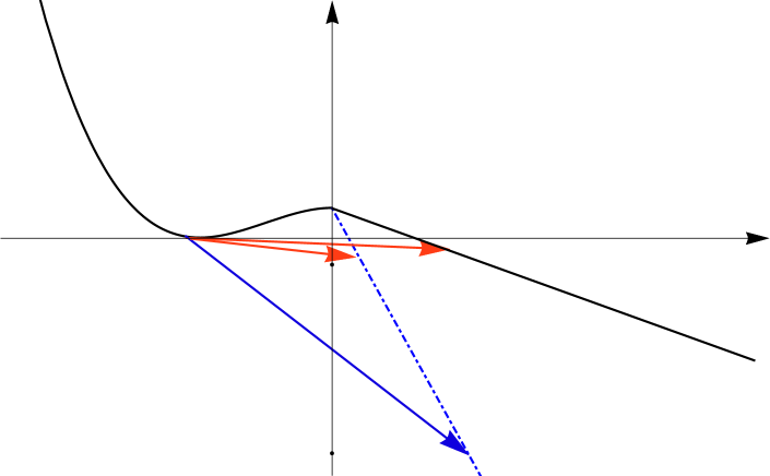
$\varphi_{f}$

$V$

$\varphi$

$-V_{bar}$

$E\simeq 1$

$-\varphi_{f}^{4}$

$V_{bar}$

$\lambda_{-}\ll\lambda+$

$\lambda_{-}>1$

Figure 6: In the case of the flat linear potential with $\lambda_{-}\ll\lambda_{+}$ only the thin-wall instantons with $\left|V_{uv}\right|<\left|V_{bar}\right|$ represented by the red solid line exist. The limiting case $\left|V_{uv}\right|\simeq\left|V_{bar}\right|$ corresponds to the Coleman instanton. For the steep potential with $\lambda_{-}>1$, both the friction-dominated and thin-wall instantons exist. The lower blue line shows the transition for the friction-dominated instanton to the lowest possible value of the potential in the quantum core corresponding to $E\simeq 1$. For the Coleman instanton, which also exists in this case, $E\ll 1$, and thus it is completely saturated by quantum fluctuations.

6.2 Linear potential

The methods developed in this work can be applied with an obvious modification to a much broader class of potentials, namely, the potentials with two minima and the potentials which are not necessarily concave. To demonstrate how this can be done in cases other than those presented above, now we consider the linear potential

$$V\left(\varphi\right)=\left\{\begin{array}[]{cc}\frac{\lambda_{+}}{4}\left(\varphi-\varphi_{f}\right)^{4}&\text{for }\varphi<0\\ \lambda_{-}\varphi_{f}^{3}\varphi+V_{bar}&\text{for }\varphi>0\,,\end{array}\right.$$ (74)

for which we can compare the approximate expressions derived by the methods of this work with the results obtained from exact solutions constructed in [4]. Here, $\varphi_{f}<0$, the coupling constants $\lambda_{+}$ and $\lambda_{-}$ are positive, the potential has the hight

$$V_{bar}=\frac{1}{4}\lambda_{+}\varphi_{f}^{4}$$ (75)

and the first derivative of the potential is discontinuous at $\varphi=0$ (see Fig.6). Depending on the ratio of the coupling constants, we can have different types of instantons and therefore we consider two limiting cases separately. As before, we will skip all numerical coefficients and focus on the parametric dependence of the instanton solutions.

a) Flat potential ($\lambda_{-}\ll\lambda_{+})$. In this case, the magnitude of the derivative of the potential $\left|V^{\prime}\right|$ as a function of $\varphi$ is shown in Fig.7. As can be seen from this figure for $E<1/\lambda_{+}$, the friction term (see the green dotted curve) dominates everywhere and the corresponding instantons cannot be regularized by quantum fluctuations. In fact, for them the time derivative $\left|\dot{\varphi}\right|$ behaves as $\varrho^{-3}$ at small $\varrho$ and the classical field dominates over quantum fluctuations everywhere up to a singularity at $\varrho=0$. Therefore, these instantons do not contribute to the vacuum decay rate. For the non-singular solutions, the potential always dominates at negative $\varphi$ and we can apply formulas (50) to estimate $\varrho_{0}$. There is a jump of the derivative at $\varphi=0$; it becomes much smaller at $\varphi=+0$ as it was at $\varphi=-0$. If we want to avoid the dominance of the friction term directly after the $\varphi=0$ crossing, which would lead us to the singularity, we must require that

$$\frac{3}{\varrho_{0}}\left|\dot{\varphi_{0}}\right|\sim\frac{V_{bar}^{3/4}}{E^{1/4}}\leq\left|V_{+0}^{\prime}\right|=\left|\lambda_{-}\varphi_{f}^{3}\right|\,,$$ (76)

where we have used equations (49) and (50). It follows from here that only for

$$E\geq E_{C}\simeq\frac{\lambda_{+}^{3}}{\lambda_{-}^{4}}$$ (77)

the instantons are non-singular. These instantons fulfil the thin-wall criterion and therefore one can apply formulas (59), which in this case lead to

$$\varrho_{0}\sim\frac{1}{\left|\varphi_{f}\right|}\left(\frac{E}{\lambda_{+}}\right)^{1/4},\quad V_{uv}\sim-V_{bar}\left(\frac{E_{C}}{E}\right)^{1/4},\quad S_{E}\sim E_{C}\left(\frac{E}{E_{C}}\right)^{3/4},$$ (78)

where we have taken into account that $\varphi_{uv}\simeq\left(\lambda_{+}/\lambda_{-}\right)\varphi_{f}$ as it follows from $V\left(\varphi_{uv}\right)\simeq 0.$ The minimum value $E=E_{C}$ corresponds to the instanton with the Coleman boundary condition that exists in this case.

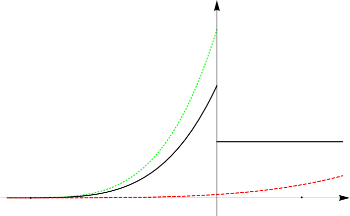
$|V^{\prime}|$

$\varphi$

$\varphi_{uv}$

$\varphi_{f}$

$\lambda_{+}|\varphi_{f}|^{3}$

$\lambda_{-}|\varphi_{f}|^{3}$

friction

Figure 7: The green dotted line describes the singular instantons for which the friction term dominates for both negative and positive values of $\varphi$. For non-singular instantons the friction term calculated in (34) under the assumption that it dominates (see the red dashed line) is always below the $\left|V^{\prime}\right|$-curve at negative $\varphi$ and it remains less relevant than the potential at positive $\varphi$ only if the condition (77) is fulfiled.

a) Steep potential ($\lambda_{+}\ll\lambda_{-})$. The magnitude of the derivitave of the potential for this case is shown in Fig.8. The derivative also jumps at $\varphi=0,$ but unlike to the previous case it becomes much larger at $\varphi=+0$ than it is at $\varphi=-0$. Therefore, here there exist nonsingular solutions describing instantons dominated by friction at $\varphi<0.$ Taking into account (34), we can see from Fig.8 that the instantons with $E<1/\lambda_{-}$ are also dominated by friction at $\varphi>0$ and are therefore singular. The non-singular instantons with

$$\frac{1}{\lambda_{-}}\ll E\ll\frac{1}{\lambda_{+}}\,,$$ (79)

are then described by expressions in (56), where we have to set $\varphi_{m}=0$:

$$\varrho_{0}\sim\frac{E^{1/2}}{\left|\varphi_{f}\right|}\,,\quad V_{uv}\sim-\frac{\varphi_{f}^{4}}{E}\,,\quad S_{E}\sim E\,.$$ (80)

The minimal value $E\simeq 1/\lambda_{-}$ corresponds to the Coleman instanton. Note that for a very steep potential with $\lambda_{-}>1$ the Coleman instanton with $E<1$ is entirely saturated by quantum fluctuations. In this case, in formulas (80) $E$ must be taken greater than unity and thus the minimal value of the potential in the quantum core is about $V_{uv}\sim-\varphi_{f}^{4}$ and the minimal size of the bubble, which should be the main contributor to the decay rate for the unbounded potential, is $\varrho_{0}\sim 1/\left|\varphi_{f}\right|$.

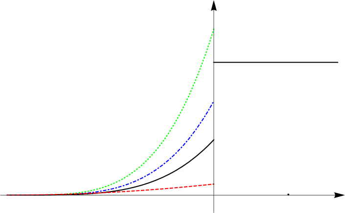
$|V^{\prime}|$

$\varphi$

$\varphi_{uv}$

$\varphi_{f}$

$\lambda_{-}|\varphi_{f}|^{3}$

$\lambda_{+}|\varphi_{f}|^{3}$

singular instantons

friction dominated instantons

thin-wall approximation

Figure 8: For very steep linear potentials with $\lambda_{-}>1$ we have, depending on $E$, the singular, the friction-dominated and the thin-wall instantons. They correspond to the dotted green, dot-dashed blue and dashed red curves, respectively. The Coleman instanton, which also exists in this case, does not belong to the spectrum because $E<1$ and this instanton is thus completely saturated by quantum fluctuations.

For $E\gg 1/\lambda_{+}$, the thin-wall formulas (59) are valid and taking into account that $\varphi_{uv}\simeq\left(\lambda_{+}/\lambda_{-}\right)\varphi_{f}\ll\varphi_{f}$, we obtain

$$\varrho_{0}\sim\frac{1}{\left|\varphi_{f}\right|}\left(\frac{E}{\lambda_{+}}\right)^{1/4}\,,\quad V_{uv}\sim-\frac{V_{bar}}{\left(\lambda_{+}E\right)^{1/4}}\,,\quad S_{E}\sim\frac{\left(\lambda_{+}E\right)^{3/4}}{\lambda_{+}}\,.$$ (81)

One can easily verify that the above formulas reproduce all the limiting cases derived from the exact solutions in [4] .

7 Conclusions

In this work, we have shown that quantum fluctuations play an important role when we consider the decay of a false vacuum. In particular, they regularize the classical instanton solutions, which would otherwise be singular. This in turn leads to the appearance of the full spectrum of new instantons, all of which contribute to the decay of the false vacuum. In those cases, when instantons with the Coleman boundary conditions exist, they normally belong to this spectrum. However, as we have seen in the example of the steep linear potential, there are potentials where the Coleman instantons are completely saturated by the quantum fluctuations and thus are no longer trustworthy as classical solutions. Moreover, we proved in [7] that for a broad class of potentials, where the false vacuum must obviously be unstable, the Coleman instantons do not exist at all. For these potentials, the decay of the vacuum is fully due to our new instantons, which actually are bouncing solutions regularized by the ultraviolet cutoff, which is self-consistently expressed in terms of the new instanton parameters.

The complete set of new instantons are classical solutions of equation (7) with the bounce boundary conditions $\dot{\varphi}\left(\varrho_{b}\right)=0$ and $\varphi\left(\varrho\rightarrow\infty\right)=\varphi_{f}$, which are reliable only within the range $\varrho_{uv}<\varrho<\varrho_{ir}$, where the ultraviolet and infrared cutoff scales are two different solutions of equation (14). At $\varrho<\varrho_{uv}$, the bubble is filled by dominant vacuum fluctuations with the ground state level shifted to $V_{uv}$. The proposed boundary conditions comprises a free parameter $\varrho_{b}$, which parametrizes the new instantons, however they in fact were parametrized by the parameter $E$ instead of $\varrho_{b}$, which is a number of quanta on the bubble size scale, i.e. $E\equiv\dot{\varphi}^{2}\varrho_{0}^{4}$, and it is more suitable for the purpose of the present paper. It is clear that for any given potential the parameter $\varrho_{b}$ can uniquely be expressed in terms of $E$ and vice versa.

In Section 5, we developed a general new method for constructing the approximate instanton solutions for arbitrary potentials, which generalizes the well known method of the thin-wall approximation [1] and actually allows to derive solutions outside of the validity of the thin-wall approximation. In the leading order, the size of the instanton, its on-shell action and the potential within the quantum core are presented either in formulae (56) or (59), depending on $E$. These characteristics of the false vacuum decay are explicitly expressed in terms of the parameters that characterize the potential, namely its hight, the position of the false vacuum, and the coupling constants.

We have applied these formulas for the concave unbounded potentials and derived in a very simple way the parametric dependence of the characteristics of the instantons for a broad class of potentials which drop as $-\varphi^{n}$ with $n\geq 4$. It has been shown that in the case of the quartic potential, for which there exists an exact solution [3], we have correctly reproduced, up to the numerical coefficients of the order of unity, all the limiting cases elaborated in [3] as a result of rather lengthy and tedious calculations. Although the numerical coefficients can be quite large, as for example in the action $\frac{8\,\pi^{2}}{3\,\lambda_{-}}$, the accuracy of our method does not allow us to estimate them reliably. Therefore, we have focused on the parametric dependences of the solutions and ignored the numerical factors, which can easily be computed numerically for a given class of potentials by considering only a single concrete set of parameters. Moreover, our method has allowed us to obtain the dependence on the parameters even in those cases for which the analytical solutions are not known, i.e., such as for $-\varphi^{6}$ and other potentials. Our proposed method is applicable to obtain the results in the leading order practically for arbitrary potentials. The key element of this method is the “master” figure, in which the dependence of the magnitude of the derivative of the potential is compared with the value of the friction term as a function of $\varphi$ calculated under the assumption that this term dominates over the potential term in equation (7). In this way we can find out which term in equation (7) can be neglected, which in turn considerably simplifies the approximate solution in the corresponding range of $\varphi$. We have shown how to apply our method to the linear potential considered in the paper [4] and have reproduced its main results in a few lines.

Acknowledgments

The work of V. M. was supported by the Germany Excellence Strategy—EXC-2111—Grant No. 39081486.

The work of A. S. was supported in part by RFBR grant No. 20-02-00411.

References

• [1] S.Β R.Β Coleman, The Fate of the False Vacuum. Semiclassical Theory, Phys.Β Rev.Β D 15 (1977) 2929 Erratum: [Phys.Β Rev.Β D 16 (1977) 1248]. doi:10.1103/PhysRevD.15.2929, 10.1103/PhysRevD.16.1248.
• [2] S.Β R.Β Coleman, V.Β Glaser, and A.Β Martin, Β Action Minima Among Solutions to a Class of Euclidean Scalar Field Equations, Commun.Β Math.Β Phys.Β 58 (1978) 211. doi:10.1007/BF01609421
• [3] V. F. Mukhanov, E. Rabinovici, A. S. Sorin, Quantum Fluctuations and New Instantons II: Quartic Unbounded Potential, Fortsch.Β Phys.Β 69 (2021) 020101 doi:10.1002/prop.202000101 [arXiv:2009.12444 [hep-th]].
• [4] V. F. Mukhanov, E. Rabinovici, A. S. Sorin, Quantum Fluctuations and New Instantons I: Linear Unbounded Potential, Fortsch.Β Phys.Β 69 (2021) 020100 doi:10.1002/prop.202000100 [arXiv:2009.12445 [hep-th]].
• [5] V. Mukhanov, Physical Foundations of Cosmology, Cambridge University Press (2005).
• [6] V. Mukhanov, S. Winitzki, Introduction to Quantum Effects in Gravity, Cambridge University Press (2007).
• [7] V. F. Mukhanov, A. S. Sorin, On the Existence of the Coleman Instantons, arXiv:2104.12661 [hep-th].