Towards Precision Cosmology With Improved PNLF Distances Using VLT-MUSE
I. Methodology and Tests

Abstract

The [O III] $\lambda 5007$ Planetary Nebula Luminosity Function (PNLF) is an established distance indicator that has been used for more than 30 years to measure the distances of galaxies out to $\sim 15$ Mpc. With the advent of the Multi-Unit Spectroscopic Explorer on the Very Large Telescope (MUSE) as an efficient wide-field integral field spectrograph, the PNLF method is due for a renaissance, as the spatial and spectral information contained in the instrument’s datacubes provides many advantages over classical narrow-band imaging. Here we use archival MUSE data to explore the potential of a novel differential emission-line filter (DELF) technique to produce spectrophotometry that is more accurate and more sensitive than other methods. We show that DELF analyses are superior to classical techniques in high surface brightness regions of galaxies and we validate the method both through simulations and via the analysis of data from two early-type galaxies (NGC 1380 and NGC 474) and one late-type spiral (NGC 628). We demonstrate that with adaptive optics support or under excellent seeing conditions, the technique is capable of producing precision ($\lesssim 0.05$ mag) [O III] photometry out to distances of 40 Mpc while providing discrimination between planetary nebulae and other emission-line objects such as H II regions, supernova remnants, and background galaxies. These capabilities enable us to use MUSE to measure precise PNLF distances beyond the reach of Cepheids and the tip of the red giant branch method, and become an additional tool for constraining the local value of the Hubble constant.

1 Introduction

Ciardullo et al. (1989) demonstrated that the [O III] $\lambda 5007$ luminosity function (LF) of planetary nebulae (PNe) in nearby galaxies has a bright upper limit. That limit, which is $\sim 640L_{\odot}$, is nearly universal across all galaxies and can therefore be exploited as a distance indicator (e.g., Jacoby et al., 1990; Ciardullo et al., 2002a). In fact, a careful comparison of the distances to $\sim 20$ galaxies within $\sim 10$ Mpc shows that the accuracy and precision of the planetary nebula luminosity function (PNLF) method is comparable to that obtainable from the tip of the red giant branch (TRGB) and Cepheids (Ciardullo, 2012, 2013). However, as initially implemented with narrow-band filter imaging, the PNLF technique begins to have difficulties beyond $\sim 10$ Mpc and reaches its effective limit by $\sim 20$ Mpc. Consequently, for the past couple of decades, the application of the PNLF to cosmological questions has been limited.

With the increasing tension between the Hubble Constant ($H_{0}$) derived from the distance ladder (e.g., Riess et al., 2019; Breuval et al., 2020; Freedman et al., 2020) and $H_{0}$ derived from early Universe measurements (Hinshaw et al., 2013; Planck Collaboration et al., 2020), a revitalization of the PNLF is worth considering as the method could be used as an alternative to Cepheid and the TRGB measurements. However, to be competitive in this era of precision cosmology, the method’s accuracy beyond 10 Mpc must be improved, and its effective limit pushed beyond 20 Mpc.

Ideally, one would like to obtain PNLF distances to galaxies in a clean Hubble flow. This presents a problem for the method, as the technique is most easily applied to early-type galaxies which are preferentially found in clusters. Unfortunately, the local potential of a typical cluster introduces a non-cosmological component to the radial velocity that is roughly $\sim$1000 km s^-1 (Ruel et al., 2014). Even if a dozen cluster galaxies are observed, this peculiar motion would still introduce a major uncertainty into any $H_{0}$ calculation. The alternative is to target isolated field galaxies, where the bulk velocity uncertainty is much smaller, of the order of $\sim 300$ km s^-1 (Scrimgeour et al., 2016). Most large field galaxies are spirals, and, though the PNLF method can be applied to these systems (Ciardullo et al., 2002a), care must be taken to remove H II regions and supernova remnants from the PN sample. Moreover, a 1% determination of the Hubble Constant requires measuring field galaxies at a distance of $\sim 400$ Mpc; this is far beyond the reach of the PNLF.

Nevertheless, there are a number of relatively nearby early-type galaxies that are not within large galaxy clusters, and, with care, PNLF distances can be obtained to spirals and other star-forming galaxies. It is therefore reasonable to try to extend the technique with modern telescopes and instrumentation. For example, a galaxy at $\sim 50$ Mpc will have a $\sim$2.5% error in $H_{0}$ due solely to peculiar motion. If a typical PNLF distance carries a statistical uncertainty of 5%, then the total error associated with 10 $D\sim 50$ Mpc galaxies would be roughly 2%. Such a precision would be interesting with regard to the problem of the Hubble Constant tension. Moreover, if the PNLF can be shown to be reliable at these larger distances, then it can be used to calibrate the luminosities of Type Ia supernovae (SN Ia) in early-type galaxies and in systems beyond the reach of Cepheids and the TRGB.

The Multi-Unit Spectroscopic Explorer (MUSE) optical integral field spectrograph (IFS) (Bacon et al., 2010) on the 8.2 m Very Large Telescope (VLT) enables this type of observation. There are several ways in which MUSE improves upon previous PNLF studies:

1. The VLT offers a larger aperture, as it has four times the collecting area of the 4-m class telescopes used in most earlier PNLF works.

2. The Paranal Observatory site frequently delivers much better seeing than $1\farcs 2$, which was the typical image quality of the previous work. The ground-layer adaptive optics system (GLAO) available for MUSE further enhances the capability to deliver data with high image quality.

3. MUSE delivers an effective bandpass that is more than five times narrower than what is typically provided by interference filters. Since PNLF measurements are background dominated, the reduced noise substantially improves the detectability and photometric accuracy of planetary nebulae.

4. Since MUSE covers the spectral range between 4800 Å and 9300 Å and has a resolution of $R\sim 2000$ at 5000 Å, it produces a spectrum for every emission-line object in its field. Contaminating objects such as H II regions, supernova remnants (SNRs) and background galaxies (such as Ly$\alpha$ emitters) can immediately be identified, thus preventing them from skewing the PNLF statistics.

5. MUSE spectra can allow spatial blends to be identified, enabling the emission from two merged sources, such as PN pairs, to be disentangled.

6. Because MUSE does not require a narrow-band filter, all PNe have the same photometric throughput, independent of their velocity. In contrast, narrow-band filters, when placed in the fast beams of large telescopes, generate a system throughput that depends on the velocity of the emission-line object being observed. This introduces a photometric error that depends on a galaxy’s rotation curve and velocity dispersion (Jacoby et al., 1989).

PNLF distances rely on accurate [O III] $\lambda 5007$ photometry of planetary nebulae superimposed on the bright continuum surface brightness of their host galaxy. Roth et al. (2004) have demonstrated that an IFS is capable of delivering accurate spectrophotometry of point sources by observing PNe in the bulge of M31 with the PMAS at the Calar Alto 3.5 m telescope (Roth et al., 2005), the MPFS at the 6 m BTA in Selentchuk (Sil’chenko & Afanasiev, 2000), and INTEGRAL at the WHT (Arribas et al., 1998). In the M31 pilot study, it was also serendipitously discovered that spectral information, specifically the H$\alpha$ and the [S II] $\lambda\lambda 6717,6731$ emission lines, facilitates the identification and exclusion of interloping supernova remnants. However, the sizes of the first generation integral field units (IFUs) were far too small to cover the field-of-view needed to obtain PNLF measurements (e.g., the PMAS field-of-view was only $8\times 8$ arcsec²).

With its much larger field of view of 1 arcmin², MUSE overcomes this limitation. For example, Kreckel et al. (2017) (henceforth Kr2017) used $\sim 45$ min MUSE exposures to identify 63 PNe in a small section (three $1\arcmin\times 1\arcmin$ pointings) of the large face-on spiral NGC 628. These authors reported a PNLF distance modulus of $(m-M)_{0}=29.91^{+0.08}_{-0.13}$ ($9.6^{+0.4}_{-0.6}$ Mpc), which is 0.26 mag larger than that found by Herrmann et al. (2008) using PNe identified with narrow-band filters. The authors ascribed the offset to MUSE’s ability to discriminate PNe from supernova remnants.

More recently, Spriggs et al. (2020) (hereafter Sp2020) extended PNLF measurements with MUSE out to the Fornax cluster, and obtained distances to the early-type galaxies of NGC 1380 and NGC 1404 (FCC 167 and FCC 219 in their nomenclature). Using Moffat profile PSF-fitting photometry as introduced by Kamann et al. (2013), these authors obtained PN magnitudes that are on average 0.4 mag fainter than corresponding measurements by Feldmeier et al. (2007) and McMillan et al. (1993), and hence inferred larger PNLF distances than the previous studies. Given these developments, it is worthwhile to explore the potential of PN observations with MUSE across a larger sample of galaxies.

In this work, we demonstrate the effectiveness of MUSE for improving distances to previously studied galaxies. We will show consistency with earlier work, we will derive distances to galaxies that were previously beyond the reach of the PNLF, and we demonstrate that it is possible to reliably measure distances to late type galaxies, thus extending the calibration of Type Ia supernovae beyond that performed by Feldmeier et al. (2007). This study focuses on the methodology. In a forthcoming paper, we will address the large set of galaxies currently in the MUSE archives. For now, we concentrate on two galaxies for which recent PNLF results exist in the literature, NGC 628, and NGC 1380. The analyses of these objects will allow us to benchmark the capabilities of MUSE PN observations against the results obtained by other distance scale techniques. In addition, we also examine the archival data for NGC 474, to confirm that MUSE can obtain PNLF distances to galaxies that are beyond the reach of Cepheid and TRGB measurements.

Table 1: MUSE Exposures of the Galaxies

Galaxy	Date	Time	seeing	Texp	Program ID	Object ID	Notes
Name			(arcsec)	(s)
NGC 628	2014-10-31	03:39:58	0.77	2535	094.C-0623	NGC628-1	(1)
	2014-10-31	04:43:34	0.83	2535	094.C-0623	NGC628-2	(1)
	2015-09-15	05:00:36	0.76	2970	095.C-0473	NGC0628-P1	(1)
	2017-07-22	07:36:36	1.14	2970	098.C-0484	NGC0628-P2	(1)
	2017-11-13	03:43:55	0.95	2970	098.C-0484	NGC0628-P3	(1)
	2017-09-16	04:17:21	1.08	2970	098.C-0484	NGC0628-P4	(1)
	2016-12-30	01:01:36	1.05	2970	098.C-0484	NGC0628-P5	(1)
	2016-10-01	04:56:15	0.69	2970	098.C-0484	NGC0628-P6	(1)
	2016-10-01	06:08:16	0.70	2970	098.C-0484	NGC0628-P7	(1)
	2017-07-21	08:25:54	0.82	2970	098.C-0484	NGC0628-P8	(1)
	2017-11-13	01:22:45	0.96	2970	098.C-0484	NGC0628-P9	(1)
	2017-11-13	02:33:10	0.75	2970	098.C-0484	NGC0628-P12	(1)
NGC 1380	2016-12-31	03:19:12	0.74	720	296.B-5054	FCC167_CENTER	(2)
	2016-12-31	03:37:29	0.88	720	296.B-5054	FCC167_CENTER	(2)
	2016-12-31	03:51:26	0.76	720	296.B-5054	FCC167_CENTER	(2)
	2016-12-31	04:09:45	0.55	720	296.B-5054	FCC167_CENTER	(2)
	2016-12-31	04:23:44	0.45	720	296.B-5054	FCC167_CENTER	(2)
	2017-01-20	02:18:59	0.93	600	296.B-5054	FCC167_MIDDLE	(2)
	2017-01-20	02:52:43	0.91	600	296.B-5054	FCC167_MIDDLE	(2)
	2017-01-20	03:09:31	0.83	600	296.B-5054	FCC167_MIDDLE	(2)
	2017-11-10	04:03:05	1.46	600	296.B-5054	FCC167_MIDDLE	(2)
	2017-11-10	04:15:03	1.43	600	296.B-5054	FCC167_MIDDLE	(2)
	2016-12-30	02:29:24	0.85	600	296.B-5054	FCC167_HALO	(2)
	2016-12-30	02:45:41	1.05	600	296.B-5054	FCC167_HALO	(2)
	2016-12-30	02:57:37	0.96	600	296.B-5054	FCC167_HALO	(2)
	2017-01-20	01:11:54	1.02	600	296.B-5054	FCC167_HALO	(2)
	2017-01-20	01:28:14	0.81	600	296.B-5054	FCC167_HALO	(2)
	2017-01-20	01:40:14	0.73	600	296.B-5054	FCC167_HALO	(2)
NGC 474	2019-01-02	10:34:21	0.65	37312	099.B-0328	WFM-NGC474-S	(1)

Note. — (1) fully reduced data cube retrieved, (2) raw data retrieved and re-reduced.

2 Observations

For this initial demonstration, we used the publicly available, fully reduced MUSE data cubes (see Romaniello et al., 2018) in the ESO Archive to derive PNLFs across a range of galaxy types and distances. We did not sift through the archive completely, but rather, we selected three representative systems that are amenable for analysis and validation of our methodology. A follow-up paper will address more galaxies. Our archive search was facilitated by the graphical user interface with ancillary data that is accessible through the ESO Portal for registered users. Because the MUSE data cubes were obtained from a variety of programs that were executed at the VLT between 2016 and 2019, the data are inhomogeneous and sample a wide range of observing conditions, with seeing measurements between $0\farcs 65$ and $1\farcs 1$ and exposure times between 0.25 and 10 hours. This heterogeneity is particularly useful for exploring the capabilities and limitations of MUSE for PNLF measurements. In one case (NGC 1380), we discovered that the semi-automatic pipeline used for creating the reduced archival data products had not worked as expected, due to the lack of bright field stars available for positional reference. This caused the individual exposures to be combined with incorrect offsets, and produced a final data cube whose image quality was a factor of two worse than those of the individual frames. For this particular data set, we retrieved the raw FITS files that are also available from the ESO Archive and re-reduced a subset of the data to restore the expected quality. Table 1 summarizes the archival data sets used for this paper.

3 Data Reduction and Analysis

Most classical PNLF measurements were performed with direct imaging cameras employing narrow-band filters, and most were mounted at the prime focus of 4 m class telescopes. As we wish to investigate the capabilities and limitations of IFS for PNLF distance determinations, it is useful to remember that the images that will be shown in this paper have been extracted from MUSE data cubes. These cubes were created via a complex process which involved the data reduction and analysis of roughly 90 000 raw spectra that were projected onto 24 CCD cameras and mounted to 24 spectrograph modules. In what follows, we describe this process in some detail.

3.1 Data Reduction Pipeline

A description of the most recent version of the MUSE data reduction software (DRS) for science users is given in Weilbacher et al. (2020). Previous versions and software development aspects are discussed in Weilbacher et al. (2014). The DRS pipeline chiefly consists of basic processing and post-processing. Basic processing includes the tasks of marking bad pixels, bias subtraction, master/sky flatfield correction, and wavelength calibration. Unlike other pipelines for fiber-based IFUs, there is no step for the tracing and extraction of spectra. Instead of performing multiple interpolations, the MUSE DRS creates a pixel table that maintains the integrity of CCD pixels by assigning each one a unique wavelength and sky coordinate. The pixel table is the output of basic processing. The post-processing step merges the data sets from the 24 spectrograph modules into one file, performs the sky subtraction, applies velocity corrections, performs the astrometric and flux calibration, and mosaics the different exposures (which may have different ditherings and rotations) into one dataset. A resampling algorithm then creates the final data product as an NAXIS=3 FITS format data cube. The output FITS file comes with two extensions: the first contains the actual data, and the second provides the variance. A summary of performance parameters is given in Table 2. For a full discussion, see Weilbacher et al. (2020).

Table 2: MUSE Data Reduction Software Performance

Parameter	Value
Bias subtraction residuals	$\leq$ 0.1 e-h-1, Note (1)
Pixel table wavelength calibration accuracy	0.01 — 0.024 Å  (0.4 – 1.0 km s-1)
Data cube wavelength calibration accuracy	0.06 — 0.08 Å  (2.5 — 4.0 km s-1)
Sky subtraction accuracy	1% at 500 nm
Flux calibration accuracy	2% at 500 nm
Astrometric accuracy (relative)	$0\farcs 05$ in RA, $0\farcs 03$ in DEC

Note. — (1) measured in units of dark current per pixel.

3.2 Differential Emission Line Filtering on Data Cube Layers

Although PNe are intrinsically bright, and a large fraction of their luminosity is radiated in the [O III] $\lambda 5007$ emission line, their signal is totally swamped in broadband images by the continuum surface brightness of their host galaxy. To detect this line, the PNLF distance technique has relied on direct imaging through narrow band filters that suppress most of the continuum while transmitting the light within the passband of the filter. Jacoby et al. (1989) have explained that by creating a difference (diff) image by subtracting a scaled continuum off-band (off) image from a corresponding [O III] on-band (on) image, the continuum surface brightness is conveniently removed, and the PNe become detectable as faint point sources on a flat noise floor. Roth et al. (2018) have demonstrated that MUSE data cubes allow a synthetic implementation of the on-band/off-band technique: by co-adding selected data cube layers for a few wavelength bins around a given emission line (Doppler shifted to the systemic velocity of the galaxy) and comparing these data to an appropriately chosen off-band image, the effective filter bandwidth of the classical direct imaging technique can be reduced from 30 to 50 Å down to 4 or 5 Å. As a result, the photon shot noise contribution from the underlying galaxy is reduced by the square root of the ratio of those numbers, thereby increasing the signal-to-noise of a PN detection by a factor of $\sim$2.5. In other words, exposures with conventional narrow-band filters would have to be 6 to 10 times longer to achieve the same signal-to-noise. Obviously, this would not be practical for observing distant galaxies. Moreover, another significant improvement can be obtained via a spaxel-to-spaxel approach to flux calibration. This novel procedure can only be achieved with an IFU, and will be described below.

For the purpose of precision PN photometry, we have refined the on-band/off-band technique by creating stacks of 15 single data cube layers, each having a width of 1.25 Å. These stacks are grouped around the wavelength of the Doppler-shifted [O III] line, in order to account for a range of PN radial velocities of $\pm$500 km s^-1 centered on the systemic velocity of the galaxy. We also create a 125 Å  intermediate-bandwidth continuum image by co-adding 100 data cube layers redward of the redshifted 5007 Å emission line. From each of the 15 on layers, we subtract the normalized continuum off image to form a total of 15 diff images.

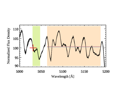
Figure 1: Left: a data cube with the on-band image (green) and the adjacent stack of off-band images (beige). Another filter variant with an additional offband stack is indicated in blue hues (see Section 3.4). Right: The relative flux of the pseudo continuum for NGC 1380, sampled at 10 different regions in the galaxy, with the wavelength intervals for on-band images (between 5029.7 and 5047.2 Å) shown in green, and the off-band image (5063.5 to 5187.2 Å) displayed in beige. The spectra show very little variation over these different regions.

As an example, the right-hand panel of Figure 1 shows the normalized spectrum of NGC 1380 measured over ten $51\times 51$ spaxel apertures that extend radially from the galaxy’s nucleus, with offsets of 10 spaxels between each sample. The on-band layers, shaded in green, are tightly related to the mean of the continuum in the off-band region, which is highlighted in beige. The latter was chosen to be close to the [O III] doublet, but away from the strong Mg b absorption feature between rest frame 5160 and 5192 Å. For reference, the wavelength of the first on-band layer is shown with a red cross. In this plot, the spectra for the 10 different apertures, normalized to the flux density at the red cross, lie almost on top of each other. The mean continuum flux, averaged over the off-band and plotted as horizontal lines, has an aperture-to-aperture standard deviation of just 0.13 %. For the calibration of each wavelength bin in the on bandpass, the continuum background at the wavelengths of Doppler-shifted [O III] emission lines can therefore be tied to the off-band with extremely high accuracy. Over the seeing disk of a point-source PN, the relation is essentially constant and even robust against surface brightness fluctuations (Tonry & Schneider, 1988; Mitzkus et al., 2018). Galaxy rotation and stellar population differences can lead to systematic shifts of the calibration constant, but as these effects generally occur on spatial scales much larger than relevant for point source photometry, they only introduce a small, locally constant residual in the background and cancel out. As will be shown below, the principle of self-referencing in each data cube spaxel is uniquely efficient for removing residual fixed pattern noise and therefore preferable over the technique of subtracting a model spectrum of the galaxy.

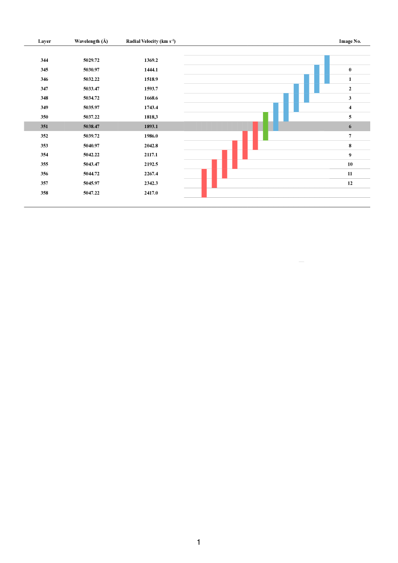
Figure 2: Data cube layers and narrow band images for NGC1380. Each layer is 1.25 Å wide, and each narrow-band image for PN detection consists of 3 adjacent layers.

Since the wavelength resolution of MUSE is roughly twice the dispersion of the data cube, the [O III] $\lambda 5007$ emission from a planetary nebulae will typically be distributed over 2 or 3 wavelength bins (layers). Thus, our method for PN detection involves summing the [O III] flux from three adjacent layers of the cube. Figure 2 illustrates this process for the Fornax lenticular galaxy NGC 1380. Here the galaxy’s systemic velocity of 1877 km s^-1 happens to fall within the 351st wavelength bin (data cube layer) and is shown as the grey shaded row. The galaxy’s internal motions then shift the 5007 Å  emission of individual PNe to wavelengths between $\sim 5030$ Å (wavelength bin 345) and $\sim 5045$ Å (wavelength bin 357), depending on the exact velocity of the object. The red and blue bars illustrate that by co-adding three adjacent layers of the data cube, 13 images are formed with effective bandpasses of 3.75 Å. This collects all the [O III] emission from all the PNe while greatly increasing the contrast of the PNe over the continuum, allowing the detection of the faintest emission-line objects relative to a narrow-band (e.g., 40 Å) image. The final photometry, however, is executed on the single layer images (Section 3.3).

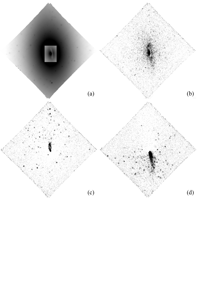
Figure 3: Continuum and narrow-band diff images of the high surface brightness nuclear region of NGC 1380, orientation: north up, east left. (a) Off-band image, note the insert that highlights a ring of dust around the nucleus, (b) diff image with a filter bandwidth of 40 Å as typically used for classical PNLF observations, (c) DELF image, blue-shifted with respect to the systemic velocity by approximately $-200$ km s^-1, (d) DELF image, red-shifted by $+200$ km s^-1. While in (c) and (d) the point-like sources are identified as PN candidates, their signal is almost completely washed out in the conventional diff image (b). The presence of a large ionized gas disk is hinted in the diff images and further discussed in Section 4.1.4.

The images shown in Figure 3 illustrate how this scheme compensates for the variation of radial velocities. The $\sim 200$ km s^-1 rotation of the galaxy (D’Onofrio et al., 1995) is clearly seen, as the PNe north of the nucleus are systematically blue-shifted, while those in the southern part of the galaxy are primarily redshifted. The effects of the galaxy’s $\sim 200$ km s^-1 velocity dispersion (D’Onofrio et al., 1995; Vanderbeke et al., 2011) are also immediately visible, as there exist a few counter-rotating objects in both regions.

To better understand the efficacy of the result, we must consider the sources of noise in the data cube. Accurate background subtraction has long been known to be a challenge for faint object spectroscopy, and the systematic errors associated with flatfield corrections are an important reason why the limit imposed by photon statistics is seldom achieved. For example, as pointed out by Cuillandre et al. (1994) for the case of long-slit spectroscopy, the limit for long exposures is not photon shot noise, but systematic multiplicative errors, caused by the CCD flatfield error $\epsilon$ (for the continuum) and slit alignment errors, $\omega$ (for strong sky line residuals). Numerically, the signal-to-noise near a sky line can be expressed as

$$\left(\frac{S}{N}\right)_{\mathrm{LS}}=\frac{I_{O}T}{\sqrt{I_{S}T+\sigma^{2}_{\mathrm{CCD}}}+(\epsilon+\omega)I_{S}T}$$ (1)

where $T$ is the exposure time, $I_{O}$ is the object flux, $I_{S}$ is the sky background flux, and $\sigma^{2}_{\mathrm{CCD}}$ is the detector noise. If $\alpha$ is the ratio between the object and sky fluxes, this term converges for long exposure times to

$$\left(\frac{S}{N}\right)_{\mathrm{LS,limit}}=\frac{\alpha}{\epsilon+\omega}$$ (2)

Adopting Equation 2 for our MUSE data, it follows that the errors from [O III] emission line spectrophotometry are strongly affected by residual flatfielding errors. As illustrated in Figure 4, these systematic uncertainties are visible as a criss-cross pattern of brightness-enhanced streaks throughout the image, with $\epsilon$ assuming values as large as 10%. This limitation was already discovered in the course of the MUSE surveys for faint Ly$\alpha$-emitting galaxies (e.g., Bacon et al., 2017; Herenz et al., 2017; Wisotzki et al., 2018; Bacon et al., 2021). Moreover, MUSE integral field spectroscopy is affected by residual errors that are more complex than the ones for long-slit spectroscopy. As pointed out by Soto et al. (2016), since the light path varies from slice to slice and from IFU to IFU, small discontinuous variations are introduced into the line-spread-function (LSF) and the wavelength solution of the final reconstructed data cube. These issues are then further exacerbated by systematic flatfielding and bias subtraction errors.

In order to remove the resulting residual patterns from deep MUSE exposures, Soto et al. (2016) invoked the ZAP filter, which is based on principal component analysis (PCA). ZAP constructs a sky residual spectrum for each individual spaxel, which can then be subtracted from the original data cube. While the method does reduce the sky residuals, it has the potential drawback that its eigenspectra, which characterize the residuals, are unable to distinguish between astronomical signals and the background. Thus the method requires very careful treatment of the filter parameters and interpretation of the filtered data.

In our application, the host galaxy background is orders of magnitude brighter than the sky, and the spectral region of interest is not plagued by bright night-sky emission lines. Under these conditions, a simple generalization of the on-band/off-band direct imaging technique is very efficient at accurately subtracting the background and suppressing the $\epsilon$-term in Equation 2.

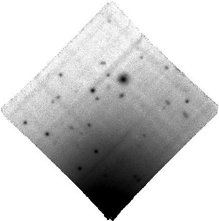
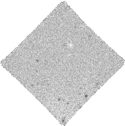
Figure 4: Example of efficient suppression of background flatfield residuals with differential emission line filtering in the HALO field of NGC 1380 (see also Fig. 15, north is up and east to the left). Left: broad-band continuum image obtained from co-adding data cube layers over the wavelength interval $5063.75\leq\lambda\leq 5188.75$ Å. The image exhibits flatfield residuals of up to 10% of the background intensity. Middle: a single data cube layer at 5045 Å, continuum-subtracted using the scaled mean galaxy spectrum to remove the pixel-to-pixel flatfield variations. Right: a continuum-subtracted single data cube layer at 5035 Å. At this wavelength, the redshifted [O III] line at 5007 Å is transmitted for PNe with a radial velocity of 1687 km s^-1, i.e., a projected velocity of $-190$ km s^-1 relative to systemic. These PNe appear as faint point sources in the image. Note that there is a hint of a local zero-point offset at the location of an unrelated $z=0.3355$ background galaxy (north of the frame center) that appears as slightly oversubtracted. This small continuum correction factor mismatch does not affect the overall flatfield of the frame nor our ability to detect PNe.

Ignoring for a moment the statistical errors that add in quadrature as well as the slit alignment error $\omega$, we can write the influence of the multiplicative systematic error $\epsilon$ on the flux measurement $F(\lambda)$ as

$$F(\lambda)=\sum_{i,j}^{N_{aper}}I_{O}(x_{i},y_{j},\lambda)-c\sum_{m,n}^{N_{skyrad}}I_{S}(x_{m},y_{n},\lambda)$$ (3)

The first term in this equation sums the apparent fluxes, $I_{0}$, in the spaxels of an object within an aperture aper; the second term does the same for the apparent spaxel fluxes, $I_{S}$, in the source’s sky annulus, skyrad. The normalizing constant $c$, which is typically $\sim 0.1$, accounts for the greater number of spaxels in the sky region. If $o$ and $s$ are the true spaxel fluxes in the object aperture and sky annulus, and $F(x_{i},y_{j},\lambda)$ is the flux per spaxel ($i$,$j$) contributing to the total, then, assuming the residual flatfield errors $\epsilon_{ij}$ and $\epsilon_{mn}$ are not varying with wavelength,

$$\begin{split}F(x_{i}.y_{j},\lambda)=(1+\epsilon_{ij})\left(o(x_{i},y_{j},\lambda)+s(x_{i},y_{j},\lambda)\right)-c/N_{aper}\sum_{m,n}^{N_{skyrad}}(1+\epsilon_{mn})s(x_{m},y_{n},\lambda)\\ =o(x_{i},y_{j},\lambda)+s(x_{i},y_{j},\lambda)+\epsilon_{ij}o(x_{i},y_{j},\lambda)+\epsilon_{ij}s(x_{i},y_{j},\lambda)-c/N_{aper}\sum_{m,n}^{N_{skyrad}}s(x_{m},y_{n},\lambda)\\ -c/N_{aper}\sum_{m,n}^{N_{skyrad}}\epsilon_{mn}s(x_{m},y_{n},\lambda)\end{split}$$ (4)

Under the assumption of a flat, or to first order, constant gradient in the background surface brightness, two terms cancel to zero, so that

$$s(x_{i},y_{j},\lambda)-c/N_{aper}\sum_{m,n}^{N_{skyrad}}s(x_{m},y_{n},\lambda)=0$$ (5)

This leaves us with three remaining terms that add a systematic error to the object flux $o(x_{i},y_{j},\lambda)$:

$$F(x_{i}.y_{j},\lambda)=o(x_{i},y_{j},\lambda)+\epsilon_{ij}o(x_{i},y_{j},\lambda)+\epsilon_{ij}s(x_{i},y_{j},\lambda)-c/N_{aper}\sum_{m,n}^{N_{skyrad}}\epsilon_{mn}s(x_{m},y_{n},\lambda)$$ (6)

The term $\epsilon_{ij}o(x_{i},y_{j},\lambda)$, which is no more than $\sim 10\%$ of the object flux, does not scale with the background surface brightness and can therefore be neglected. The two remaining terms are directly proportional to the background, meaning that deviations of $\epsilon_{ij}$ from zero can contribute a significant residual to the extracted point source spectrum whenever the background surface brightness is high.

By contrast, the difference frame method applies a scaled continuum flux subtraction within identical spaxels that are subject to the same error, $\epsilon_{ij}$. The term therefore cancels out as shown in Equation 7:

$$\begin{split}F(x_{i}.y_{j},\lambda)=(1+\epsilon_{ij})o(x_{i},y_{j},\lambda)+(1+\epsilon_{ij})s(x_{i},y_{j},\lambda)-k(1+\epsilon_{ij})\sum_{\lambda=\lambda_{1}}^{\lambda_{n}}s(x_{i},y_{j},\lambda)\\ =(1+\epsilon_{ij})\left[o(x_{i},y_{j},\lambda)+s(x_{i},y_{j},\lambda)-k\sum_{\lambda=\lambda_{1}}^{\lambda_{n}}s(x_{i},y_{j},\lambda)\right]\end{split}$$ (7)

The scaling factor $k$ can be accurately measured from the data cube itself, such that the background terms vanish:

$$s(x_{i},y_{j},\lambda)-k\sum_{\lambda=\lambda_{1}}^{\lambda_{n}}s(x_{i},y_{j},\lambda)=0$$ (8)

and we are merely left with a small error on the flux:

$$F(x_{i}.y_{j},\lambda)=(1+\epsilon_{ij})o(x_{i},y_{j},\lambda)$$ (9)

As we have verified in various tests (Section 3.6), the continuum band can be scaled to the adjacent [O III] $\lambda 5007$ window with very high accuracy, as long as there are no dramatic changes in the underlying stellar population or kinematics of the host galaxy. Such changes do not often occur over the MUSE field-of-view in early-type systems (such as NGC 1380), so the error in the scaling factor $k$ is held well below 1%. (For aperture photometry, the term is even less important: as long as there is no strong population gradient, the factor will cancel.) The middle and right panels in Fig. 4 illustrate how well the background subtraction is accomplished in practice.

Based on the above analysis, we have expanded the technique of extracting a small number of continuum-subtracted diff images and have processed the entire data cube with a tool that replaces each layer with a continuum-subtracted diff frame; this step isolates any emission features and produces a high signal-to-noise measurement with practically no background residuals. This tool has also been instrumental for measuring the emission lines of H$\alpha$ and [S II] that are important for the reliable classification of PNe (see Section 3.5 below).

To summarize, the generalization of the classical on-band/off-band technique to MUSE data cubes not only provides an advantage of much smaller filter bandwidths, hence less background flux from the host galaxy, but also reduces spaxel-to-spaxel flatfield residuals that would otherwise produce overwhelmingly large errors in regions of high host galaxy surface brightness. These two advantages allow PNLF studies to be made with greater precision and to much greater distances than previous studies. In fact, this differential emission line filter (DELF) technique is conceptually similar to using beam-switching in the near infrared, or to the nod-shuffle option in optical spectroscopy (Cuillandre et al., 1994; Glazebrook & Bland-Hawthorn, 2001; Roth et al., 2002), in the sense that identical pixels are used for comparing object + sky with sky. The main difference is that no extra exposure time is spent on sky frames.

3.3 Source detection and photometry

As described in the previous section, the detection of PN candidates and the measurement of [O III] magnitudes were accomplished by adapting the methods of classical on-band/off-band photometry to the set of diff images at different wavelengths produced from the MUSE data cubes. Our procedure consisted of four major steps.

First, the identification of PN candidates was performed visually by scanning through the set of images that were co-added over three wavelength bins. We found that loading the images into 13 consecutive frames of the DS9 tool (Joye & Mandel, 2003) and “tabbing” through the images provided a generalization of the classical blinking technique. We required all valid PN candidates to appear in at least three successive frames and have a point-source appearance. In a future tool, this requirement can be implemented in software via an source detection algorithm. However for the present work, this level of automation was not necessary. Once found, the position of each PN candidate was recorded and used as a first estimate for the next step in our analysis.

With the initial coordinate estimates in hand, the centroids of the PN candidates were measured using the GCNTRD routine, available in the NASA IDL Astronomy User’s Library. This routine fits a Gaussian to the image in all 15 frames of the unbinned diff images. Because the [O III] $\lambda 5007$ emission only appears in those few images of the stack that correspond to the PN’s radial velocity, we only measured the centroid when the flux from rough aperture photometry exceeded some threshold value above the noise. The centroid obtained from the brightest image of the series was adopted as the best ($x$,$y$) position of the PN candidate.

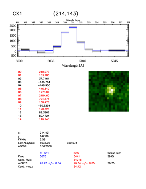
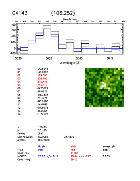
Figure 5: The short spectra for one bright and one faint PN in NGC 1380. Images of the PNe formed by co-adding 5 data cube layers centered on the brightest bin are shown on the right; the spectra formed from 15 layers of the data cube are displayed on the left. The thick black histograms show the measured DAOPHOT fluxes in each bin, while the thin black lines illustrate the photometric uncertainties. The blue histograms display the Gaussian fits. The abscissa is labeled in wavelength on the bottom and layer numbers on the top. Top row: CX1, a PN with $m_{5007}=26.43\pm 0.05$. Bottom row: PN CX143, with $m_{5007}=28.25\pm 0.17$. Gaussian fits to the two emission lines yield central wavelengths and corresponding radial velocities of 5038.06 Å/$1865.9$ km s^-1 and 5034.56 Å/$1657.6\,$km s^-1, respectively.

In step 3 of our procedure, we used the Gaussian-based centroids to perform aperture photometry in all 15 frames of the unbinned diff images, thereby creating a short 15-pixel spectrum in the relevant wavelength region of interest. We validated the photometry with two different tools (see Section 3.6). Depending on the image quality of a given data cube, we chose a DAOPHOT aperture radius of 3 pixels, or slightly larger, and a sky annulus with inner and outer radii of typically 12 and 15 pixels. Examples of two of these short spectra are shown in Figure 5.

In step four, we measured the [O III] flux by first fitting a Gaussian to the resulting emission line in the short spectrum (with the central wavelength, line full width at half maximum (FWHM), and normalization as free parameters), and then either recording the integrated flux over the fitted profile, or co-adding the individual flux measurements from the closest 5 bins around the peak of the Gaussian fit. For well-behaved profiles, the two methods yield values that agree within a few hundredths of a magnitude. However, in cases of double-lined or broadened profiles, which occurred when the images of two PNe with different radial velocities happen to overlap with each other, the flux from summing over 5 bins is significantly larger. We resolved this problem with an interactive deblending tool that fits two separate Gaussians to the data. This produced a more accurate magnitude for each component of the blend (see Section 4.1.2).

These steps were supplemented by visual inspection of both the original diff images and the short spectra produced in step four. This allowed us to immediately identify overlapping objects and assess sources corrupted by unrelated emission features or spurious signals.

To account for the flux beyond our 3 pixel radius measuring aperture, we need to apply an aperture correction using stars in the field. Given the small field of view of MUSE, most galaxy exposures in the ESO archive contain too few stars bright enough for a reliable PSF measurement using just the data layers of interest. Moreover, within the body of a nearby galaxy, it is often difficult to discriminate foreground stars from one of the galaxy’s semi-resolved globular clusters. Consequently, we need another method to measure the aperture correction for our PN measurements.

To address this challenge, we created broadband (200 Å) images from co-added data cube layers centered on the redshifted [O III] line. Point source candidates of sufficient brightness were identified with DAOPHOT FIND and ordered by apparent magnitude from their DAOPHOT APER measurements. After identifying up to 10 of the brightest stars in the field, we applied the Levenberg-Marquardt algorithm mpfit to fit their PSFs with Gaussian and Moffat functions (Markwardt, 2009). For each star, two different approaches were used for the fit: one in the off broadband wavelength region to a create high signal-to-noise measurement of the PSF. As an independent check, and also to address the wavelength dependence of aperture corrections, another fit was applied in each layer of the data cube, albeit at the expense of noisier results.

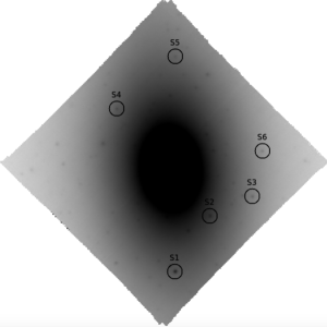
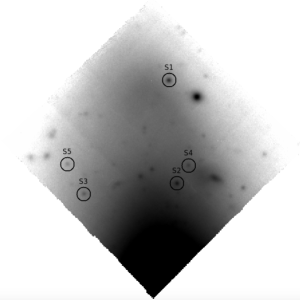
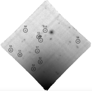
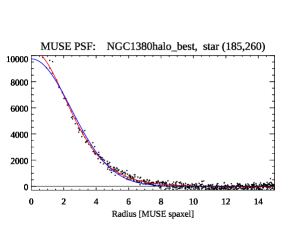
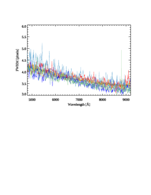
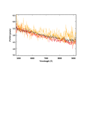
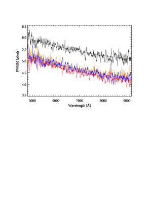
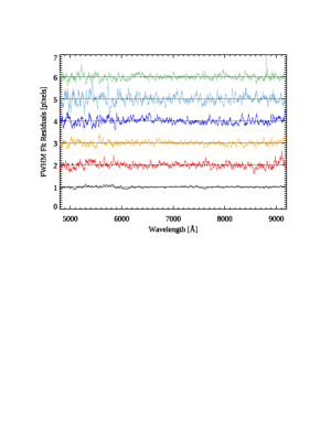
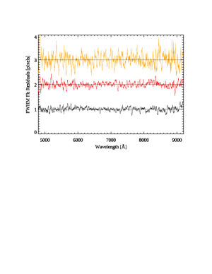
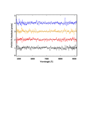
Figure 6: Examples of PSF measurements in the MUSE data cubes of NGC 1380’s CENTER (left column), MIDDLE (middle column), and HALO (right column) - see also Fig. 15. The first row shows continuum images centered on the redshifted [O III] line, with a bandwidth of 200 Å. Point sources are indicated with circles and labeled S1, S2, etc. Radial plots for the brightest point source in each field, overplotted with a Gaussian fit (blue) and a Moffat fit (red), are shown in the second row (ordinate flux units: $10^{-20}$ erg cm^-2 s^-1). Row 3 presents the FWHM for all field stars that were bright enough to yield a successful PSF fit, plotted as a function of wavelength across the data cube (ordinate units: pixels). The scatter of these values, shown as residuals from second order polynomial fits (the full drawn lines in Row 3) are plotted in Row 4 (with incremental offsets of 1 for clarity). The difference in image quality from the CENTER (4.1 pixels FWHM, $0\farcs 82$), DISK (5.4 pixels FWHM, $1\farcs 08$), and HALO (5.1 pixels FWHM, $1\farcs 02$) is obvious. Note that HALO star S1 is a resolved globular cluster and has a FWHM of 5.8 pixels, significantly larger than the other objects in this field (black curve in Row 3, right column). This source cannot be used to determine an aperture correction.

As pointed out by Kamann et al. (2013), PSF fitting parameters are expected to vary smoothly with wavelength, with the FWHM monotonically decreasing towards the red. We used this a priori knowledge to fit a second order polynomial to the measured FWHM as a function of wavelength; this model proved to be satisfactory even for very faint objects. The scatter of the residuals at the nominal wavelength of [O III], Doppler-shifted to the systemic velocity of the galaxy in question, was taken as a measure for the uncertainty of the PSF determination. Finally, for the well-behaved point sources from this analysis, aperture photometry was performed within incrementing radii, typically ranging from 3 pixels up to 12 pixels, where, as before, the sky annulus was defined using inner and outer radii of 12 and 15 pixels, respectively. The difference between the flux at 3 pixels and the asymptotic value at large radii was adopted as the aperture correction for the given data cube. The formal error for this value was estimated from the standard deviation of the residuals, again from a polynomial fit, over an interval of $\pm 100$ Å around the redshifted [O III] line.

The corresponding curves for a number of stars superposed on NGC 1380 are shown in Figure 6. This approach is, unfortunately, sensitive to contaminants: in NGC 1380, some of the “stars” are resolved on HST frames and are listed by Jordán et al. (2015) as candidate globular clusters. Thus, one must be cautious about using a blind analysis of field objects. Without further information, such as high-resolution HST imaging, a MUSE frame’s PSF may be overestimated. Object S1 in the HALO field of NGC 1380 is actually a globular cluster, as it has a significantly larger FWHM than other sources in the field and is therefore unsuitable for measuring the frame’s PSF. We note that for future targeted PNLF observations with MUSE, the pointings should be planned to ensure the presence of PSF template stars in the field.

In order to validate the stellar PSF determination as applicable for the PNe, we stacked several tens of the brightest PN images from the 3-wavelength-bin series of frames. To account for the sub-pixel offset between the point source positions, the sub-images around each object were rescaled by a factor of 10 and shifted to a common centroid. This allowed for registration to a common center that is accurate to within one tenth of a pixel ($0\farcs 02$), i.e., small enough to have a negligible affect on the PSF and aperture correction. As an example, Figure 7 shows the stacked PN images for the central field in NGC 1380 along with a radial plot of the resulting PSF.

         

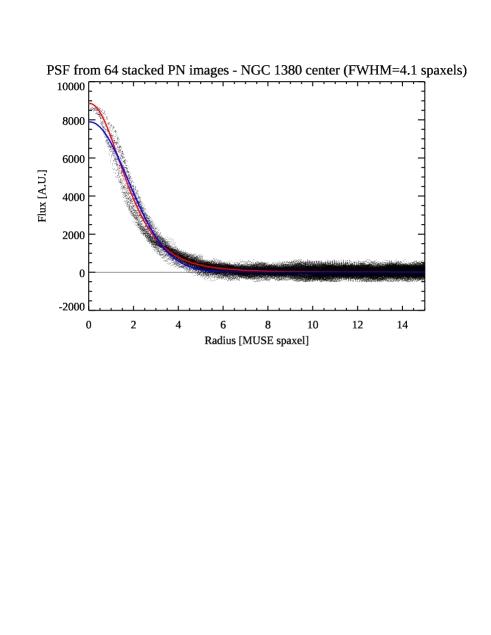
Figure 7: Left: image of a stack of the 64 brightest PNe in NGC 1380 CENTER field. Right: radial plot of the PSF. A Gaussian fit to the PSF (shown in blue) yields a FWHM of 4.1 pixel, in agreement with the analysis of the field stars. For comparison, a Moffat fit is shown in red.

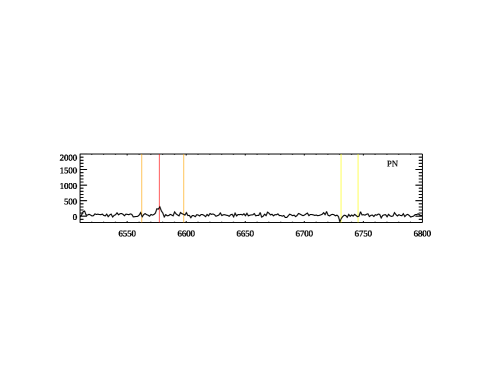
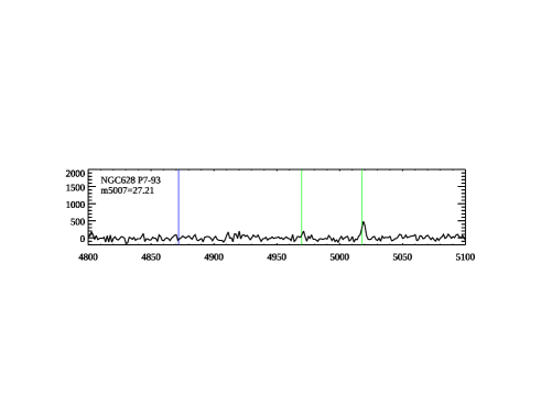
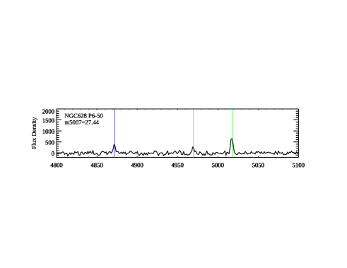
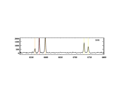
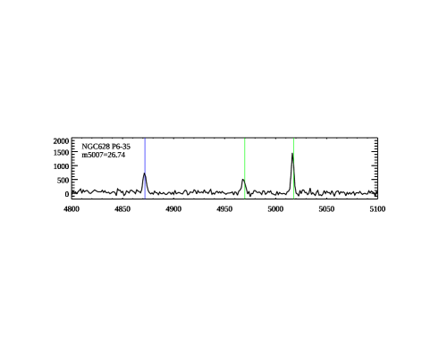
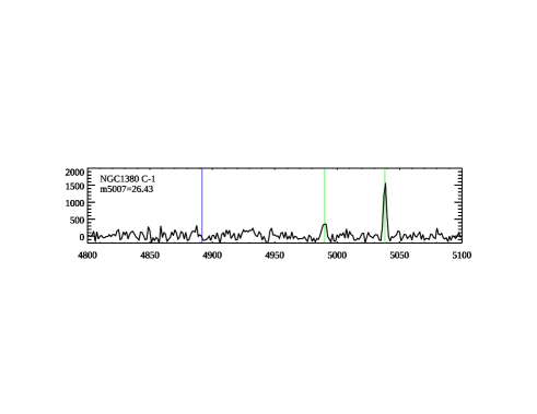
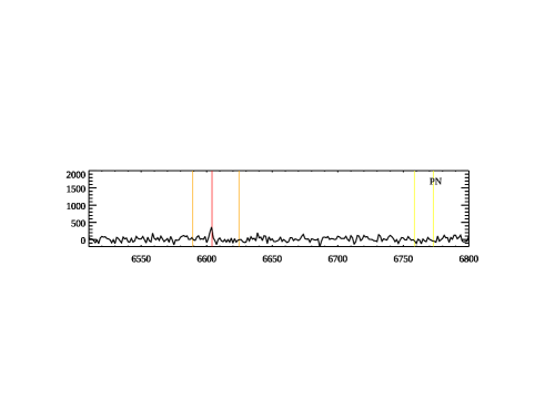
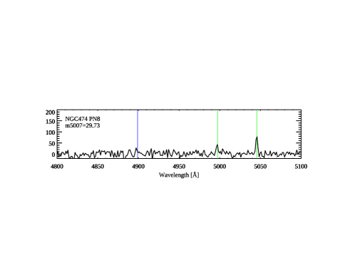
Figure 8: Example spectra, illustrating the range of brightness, and different classes of emission line objects. Flux density is plotted in units of $10^{-20}$ erg cm^-2 s^-1 Å^-1. Note that for the faintest object (Row 7) the scale is stretched by a factor of 10. The wavelengths of H$\beta$, [O III], H$\alpha$, [N II], and [S II], shifted to the systemic velocity of the host galaxy, are indicated with colored lines. The spectrum of the overluminous PN C-1 in NGC 1380, shown in Row 6, presents no peculiarities, such as split or broadened emission lines that otherwise might indicate a blend of two objects. As a curiosity, the spectrum of PN8 in NGC 474 (Row 7) shows a broad, asymmetric emission line at a wavelength of $\sim 6740$ Å. The corresponding datacube layers reveal a chance alignment of PN8 with one of two Ly$\alpha$ emitting galaxies at a redshift of $z=4.551$ (see Fig. 30).

3.4 Spectroscopy

To confirm a PN candidate, it is necessary (though not sufficient) to detect a point source at the wavelength of the [O III] $\lambda 5007$ emission line, Doppler-shifted to the systemic velocity of the galaxy, and allowing for orbital motion within the system’s gravitational potential. To rule out interlopers such as high redshift background galaxies, one generally needs to detect another emission line at the correct wavelength, typically [O III] $\lambda 4959$, or H${\alpha}$. Also, depending on the Hubble type of the host galaxy, it may be necessary to distinguish PNe from supernova remnants or H II regions — a task that is particularly critical in late type galaxies.

For this purpose, we extracted the spectrum of each PN candidate by performing DAOPHOT aperture photometry in each layer of the data cube, using the same procedure as for the determination of $m_{5007}$ magnitudes, including centroiding the line and applying (wavelength-dependent) aperture corrections. To this end, we expanded the scope of the DELF to the entire wavelength range of the data cube. This version of our code samples the continuum underlying a targeted emission line using two wavelength intervals which bracket the line of interest. This option is illustrated by highlighting the data cube layers of Fig. 1 in blue and red hues. We note that bright night sky emission lines in the regions which define the continuum can create a bias and must therefore be masked from the analysis. This feature has not yet be implemented in our software. However, since the current study does not extend to wavelengths beyond $\sim$ 7500 Å, masking was not necessary for our analysis and satisfactory results were found with the former version of the code. In problematic cases, e.g., for objects located near the edge of the field, we were able to measure spectra interactively using the P3D visualization tool. This program allows the user to select individual spaxels to represent objects and background by defining arbitrary geometries in the data cube (Sandin et al., 2010).

Figure 8 presents a few representative examples of the emission line sources detected by our analysis, including PNe of different brightness, a supernova remnant, a compact H II region, and a high redshift interloper.

3.5 Classification

The confirmation of PN candidates as true planetaries is an important task, as background galaxies, supernova remnants, compact H II regions, and even some AGN may contaminate a sample of PN candidates. If left unrecognized, these objects can distort the bright-end cutoff of the PNLF and cause an underestimate of a galaxy’s distance. While the (rare) cases of single emission line interlopers are easily flagged owing to the absence of [O III] $\lambda 4959$ and/or H$\alpha$, the spectrum of a SNR or a compact H II region is not necessarily that different from that of a PN. Furthermore, spatially overlapping PNe, which may sometimes appear as a single overly bright object in narrow-band images can be deblended spectroscopically, only if the radial velocities of the two objects differ by more than $\sim 100$ km s^-1.

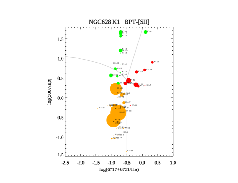
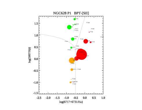
Figure 9: BPT-diagrams (Baldwin et al., 1981) for pointings K1 (left), and P1 (right)in NGC 628. The green circles are PNe, orange indicates H II regions, and red represent supernova remnants. The symbol sizes indicate the $m_{5007}$ magnitude, with larger circles representing brighter objects.

To distinguish PNe from H II regions and SNRs, we have adopted the classification scheme of Frew & Parker (2010), who plotted the [O III]/H$\beta$ line ratio against [S II]/H$\alpha$, where [S II] refers to the sum of the [S II] doublet $\lambda\lambda$ 6717, 6731 Å. This adaptation of the “BPT-diagram” (Baldwin et al., 1981) has the advantage of being insensitive to dust extinction, while still being very effective at discriminating various classes of emission-lines objects.

Figure 9 shows our BPT diagram for two fields in the face-on spiral galaxy NGC 628. The curves show the regions occupied by PNe, H II regions, and supernova remnants; three very bright H II regions in the K1 field have been deliberately included for illustration. In the figure, the symbol sizes are directly proportional to the luminosity of the [O III] $\lambda 5007$ line. We note that while the dividing line between PNe and SNR is rather well-defined and based on empirical data (Sabin et al., 2013), the separation between PNe and H II regions as defined by Kewley et al. (2001) is less clear. Although there is a sharp upper limit to the [O III]/H$\beta$ line ratio of H II regions, a considerable number of Galactic PNe fall below this line (Frew & Parker, 2010). However, the Frew & Parker (2010) study included PNe of all luminosities, while the line ratios of PNe in the brightest $\sim 1$ mag of the PNLF are considerably more homogenous (Ciardullo et al., 2002a; Richer & McCall, 2008). This fact is illustrated in the figure: objects with [O III] luminosities significantly brighter than the PNLF cutoff fall securely in the H II region area of the diagram. In contrast, the cluster of objects identified as PNe all have [O III]/H$\beta$ ratios above 5. Nevertheless, because of the PN/H II region ambiguity, we can create two versions of the PNLF, one with, and another without the borderline cases. A comparison of the resultant two distances would yield a systematic component in the uncertainty in the corresponding distance determination.

3.6 Tests

To convince ourselves that the photometry on DELF processed data cubes delivers the expected accuracy, we conducted several internal and external tests, including embedding artificial PNe of known fluxes into the observed data cubes. These tests allowed us to search for systematic photometric errors or inaccurate error estimates that could enter the PNLF distance determination algorithm, and potentially produce biased distances.

3.6.1 Differential emission line filtering

We validated the performance of the DELF technique using data cubes centered on the nuclei of galaxies. These regions have a wide range of continuum surface brightnesses, and are therefore excellent locations for testing the efficiency of our photometric techniques. NGC 1380 is a good place to begin as we can compare our own data with signal-to-noise values for PNe published by Sp2020. Figure 10 presents the results of this analysis.

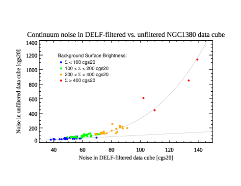
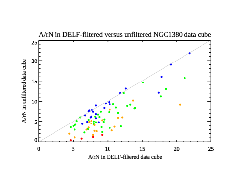
Figure 10: Test of DELF photometry on PNe projected near the center of NGC 1380. The objects are located in regions with a variety of surface brightnesses, with blue representing $\Sigma<100$, green $100\leq\Sigma<200$, orange $200\leq\Sigma<400$, and red $\Sigma\geq 400$, in units of $10^{-20}$ erg cm^-2 s^-1 Å^-1 [cgs20], as integrated over the aperture. Left: comparison of continuum noise of the unfiltered data cube versus DELF-filtered cube. Right: amplitude/residual noise ratio (ArN) for PNe measured in the unfiltered data cube versus the DELF-filtered cube.

On the left, the graph shows the residual continuum noise in the wavelength interval $5100\leq\lambda\leq 5500$ Å, measured from PNe spectra that were extracted with DAOPHOT using an aperture radius of 3 pixels and a sky annulus between 12 and 15 pixels. The noise is plotted in units of $10^{-20}$ erg cm^-2 s^-1 Å^-1 for 104 PN candidates of all brightnesses measured on both the unfiltered data cube and the DELF-processed data cube. The objects are located in regions with a variety of surface brightness. As expected, the residual continuum noise is clearly correlated with the background surface brightness. In regions of low surface brightness, the unfiltered and filtered noise levels are the same (the grey 1:1 line). However, the unfiltered noise increases rapidly as the background brightens (grey curve, representing a fourth-order polynomial). The noise levels for the DELF measurements are never worse than those for the unfiltered data, and at high surface brightness, they are far superior. We conclude that the MUSE-specific on-band/off-band technique is the preferred choice for further processing.

This is confirmed by comparing the signal-to-noise ratio of PNe magnitudes with and without filtering. We have chosen to use the quantity A/rN introduced by Sp2020, which is the ratio of the amplitude of their simultaneous fit of [O III] in the spatial and spectral domains over the residual noise of the fit. We compute the same ratio in our background-subtracted spectra by fitting a Gaussian to the [O III] $\lambda 5007$ line and measuring the noise, again in the wavelength interval $5100\leq\lambda\leq 5500$ Å. The plot on the right in Fig. 10 shows A/rN for the unfiltered data versus A/rN with the filter. The color coding is the same as for the previous test. Sp2020 considered objects measured with an A/rN below 3 to be uncertain. Our plot reveals that a considerable fraction of measurements without the filter fall below this threshold. The same measurements with the DELF technique lie well above the Sp2020 threshold. The correlation with background surface brightness is again evident.

Additional plots which directly compare our A/rN and magnitude measurements with those of Sp2020 are presented in Section 4.1. Based on these three analyses, we conclude that DELF is indeed an efficient tool for suppressing systematic flatfielding errors in MUSE emission line spectrophotometry. While this is especially important in the inner regions of galaxies where PNe are plentiful and the continuum surface brightness is high, DELF offers significant improvement even when the background surface brightness is low, as the photometric uncertainties will still be dominated by fixed pattern flat-fielding errors.

3.6.2 Photometric tests using artificial PN images

In order to check the validity of our photometry, we performed tests with artificial emission line point sources embedded in the original MUSE data cubes with a priori known positions, fluxes, and radial velocities. Running the algorithms on the original data with these mock PNe allows us to assess random and systematic errors for our photometry and spectroscopy, and determine how the detection limit for a given cube depends on the continuum surface brightness across the galaxy.

Figure 11 illustrates two examples from an extensive series of tests: frame (a) shows the distribution of a regular grid of PN positions, plotted over the halo surface brightness of NGC 1380 in the continuum. Frame (b) presents the image corresponding to the Doppler-shifted wavelength of [O III], extracted from the simulated data cube over three layers for a better signal-to-noise ratio. The grid comprises 11 groups of 11 mock PNe with magnitudes between $m_{5007}=28.0$ and $m_{5007}=29.0$ in increments of 0.1 mag, placed diagonally with decreasing brightness from upper left to lower right. Frame (c) is analogous to (a), but the PNe have random positions, random radial velocities (hence they appear in different data cube layers), and random $m_{5007}$ magnitudes in the range $27.0\leq m_{5007}\leq 29.5$.

The mock PNe were inscribed into the data cube as follows. First, a two-dimensional point source image was created using the assumption of a Gaussian PSF. A Gaussian was chosen because the details of the PSF were deemed to be unimportant, as all our photometry is performed using small (3 pixel) apertures and a sky annulus with inner and outer radii of 12 and 15 pixels. The FWHM and total flux contained in the point source were varied from run to run, with values appropriate for the specific galaxy being analyzed.

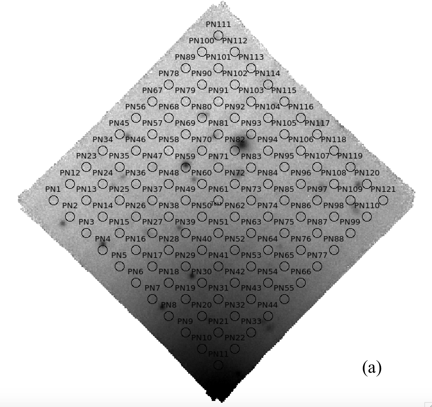
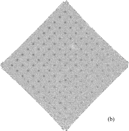
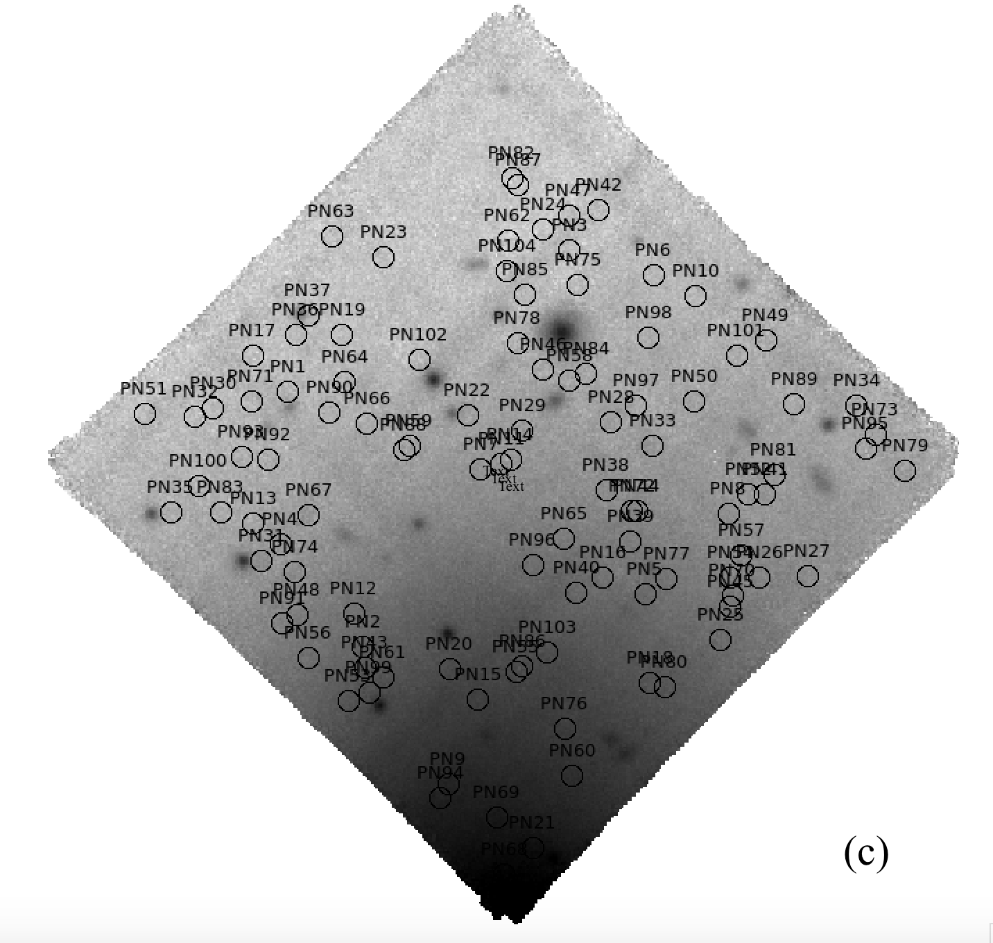
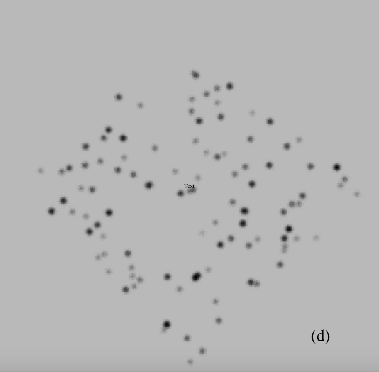
Figure 11: Simulated PN images in MUSE data cubes of the HALO field of NGC 1380. (a): regular $11\times 11$ grid of PNe with magnitudes between $28.0\leq m_{5007}\leq 29.0$ in increments of 0.1 mag. The locations where the PNe are inserted are shown via the circles. All PNe have their emission at the same wavelength. (b): image extracted from the previous cube, binned over 3 layers of wavelength. (c): mock PNe with randomly chosen magnitudes in the range $27.0\leq m_{5007}\leq 29.5$ and randomly distributed radial velocities (only positions indicated). (d) a 2-dimensional image of NGC 1380 before inserting mock PNe at different cube layers. Note the chance alignment of several overlapping PNe.

Next, the noise-free point sources, which were in units of photons per pixel, were modified with a Poissonian noise generator, using the IDL function POIDEV. These noisy images were then transformed into cgs units, and measured with DAOPHOT’s aperture photometry routine phot to determine their “true” magnitudes.

Finally, the noisy 2D-image was added into the data cube of a galaxy, either in a grid at a common wavelength or at random positions with wavelengths distributed over the 15 data cube layers that are relevant for the galaxy in question (see Section 3.2) and weighted by the Gaussian profile of the assumed MUSE line spread function (LSF). In other words, the input image with artificial PNe is projected into the stack of 15 data cube layers such that each PN has the correct LSF for its assigned Doppler-shift.

It is worthwhile mentioning that sometimes the random assignment of a PN position leads to chance superposition of objects, e.g., PN82 and PN87 in Fig. 11c, that can be hard to distinguish in a 2D-image (d). In some cases, the PNe can be resolved in the data cube by their velocity difference. However, if $\Delta v\lesssim 100$ km s^-1, the PNe may appear as one object. While this seems to be an academic exercise of the simulations, we find such examples exist in reality, and have a potential impact on the PNLF (see the discussion in Section 4.1).

The analysis of photometric simulations as dense as the one in Fig. 11c also reveals that aperture photometry is negatively influenced by the presence of too many emission line objects in the sky annuli. Such a condition causes complex cross-talk and systematic errors that are hard to remove. Since the density of bright PNe in distant galaxies is generally not high enough to trigger these problems, we conducted the remainder of our simulations using a modified position generator that reduces the number of objects per frame by imposing a minimum distance between sources (30 pixels). This constraint entirely erased the cross-talk artifacts observed in the simulations. It was subsequently chosen as the standard routine.

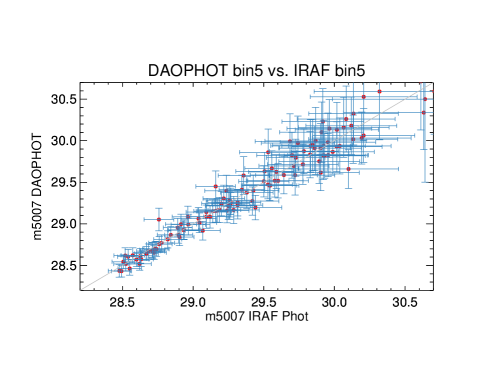
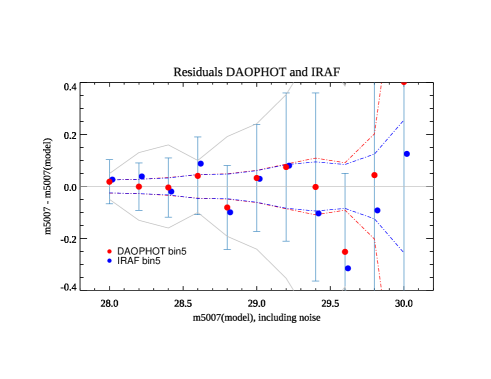
Figure 12: Comparison of aperture photometry DAOPHOT APER and IRAF-Phot with simulated PNe as illustrated in Fig. 11 (a),(b). Left: DAOPHOT magnitudes versus IRAF. Right: the mean residuals in bins of 0.2 mag. The dashed curves outline the error of the mean, while the error bars on the red symbols illustrate the typical uncertainty of a single measurement in each bin. The grey envelope outlines the standard deviation of the DAOPHOT measurements in each bin.

Using data cubes with artificial PNe placed on a grid as shown in Fig. 11a and Fig. 11b, we compared two different aperture photometry tools for internal consistency: DAOPHOT’s aper, and IRAF’s phot. The results are shown in Figure 12. The overall agreement in a magnitude range of $28.5\leq m_{5007}\leq 29.5$ is very good. We note that this test is idealized in the sense that the centroids of the point sources are accurately known a priori; this would not be the case for measurements of unknown objects, and in particular, very faint objects at the frame limit. However, the exercise is useful to demonstrate the validity of our photometry down to faint magnitudes.

The lower-right panel in Fig. 12 plots the photometric residuals for the two tools, showing average values in 0.2 mag bins. The DAOPHOT results exhibit the best agreement with the input values of the simulation. The error bars on the red symbols illustrate the typical uncertainty of a single measurement in each bin, not the error of the mean, which is plotted with dashed lines. The grey lines represent the envelope for the standard deviation of the DAOPHOT measurements in each bin; these are in reasonable agreement with the error bars of single measurements as taken from the DAOPHOT error estimates. The kink at $m_{5007}=28.6$ is an artifact of our simulation and is due to the systematics of the data cube and the fixed pattern of the grid.

In order to remove the systematic, a fully randomized simulation as highlighted in Fig. 11c and Fig. 11d was executed. Using an automated script, we generated 10000 artificial PNe and distributed the objects amongst 200 data cubes, with 50 objects per cube. The results of these models are plotted in Figure 13. The left panel shows a scatter plot of all 10000 measurements, while the plot on the right illustrates the typical $1\sigma$ uncertainties reported for individual measurements. The envelope curves indicate the measured standard deviation in each bin.

Except for the faintest magnitudes, the quantities agree well, confirming that the DAOPHOT error estimates are statistically meaningful and credible. At a magnitude of $m_{5007}=27.0$, which is slightly fainter than the PNLF’s bright-end cutoff for NGC 1380, the simulated photometry indicates individual errors of 0.04 mag. Errors of the mean, which are of order 0.01 mag, demonstrate that there is no systematic error in the photometry down to $m_{5007}\sim 28.0$. Beyond that point, a systematic offset does become apparent, and the amplitude of the systematic grows to $\sim 0.07$ mag at $m_{5007}\sim 29$, which is roughly the detection limit in the cube.

The simulations confirm that our technique yields precision spectrophotometry for point-like emission-line sources having the magnitudes of PNe at distances of $15\lesssim D\lesssim 25$ Mpc. In typical 1 hour exposures, measurements of the bright end of the PNLF should be accurate to $\sim 0.04$ mag with no apparent systematic errors, even in regions of high surface brightness. The errors can clearly be reduced and the method extended to greater distances with larger PN samples and with longer exposure times. Based on these promising results, we perform all of our photometric measurements with DAOPHOT.

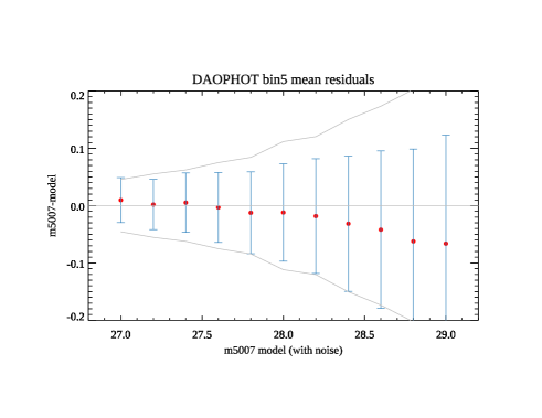
Figure 13: A simulation with 10000 artificial emission line point sources. Left: residuals of all the measurements. Right: the average residuals within 0.2 mag bins. The error bars represent the uncertainties of individual measurements, while the grey envelope sketches the standard deviation in each bin.

3.6.3 Radial velocities

The line fitting tool of our spectroscopy provides a measurement of the line-of-sight velocities of individual PNe, and thus allows for future exploration of the gravitational potentials of PN host galaxies. To test this capability, we used our simulations to assess the accuracy of the Gaussian fit to the [O III] emission line. Figure 14 shows the velocity residuals of mock data, obtained from 1000 realizations of PNe in a total of 20 data cubes, each simulating a 1 hour MUSE exposure of a galaxy. The full range of velocity residuals is the equivalent to two MUSE wavelength bins, i.e., 2.5 Å. It is immediately apparent that the velocity accuracy is on the order of one tenth of a wavelength bin, with a standard deviation of 5.0 km s^-1 for objects in the magnitude range $27.0\leq m_{5007}\leq 27.5$, 7.0 km s^-1 between $27.5\leq m_{5007}\leq 28.0$, 11.1 km s^-1 between $28.0\leq m_{5007}\leq 28.5$, and 16.4 km s^-1 for PNe fainter than 28.5 mag. The error of the mean again demonstrates that there is no systematic offset in the measurements. The simulation shows that the central wavelength error is well-behaved, and that radial velocities at the bright end of the PNLF can be measured with an accuracy of a few km s^-1. We have used this result in our subsequent analysis of benchmark galaxies for calibrating the line-of-sight velocity (LOSV) error as a function of PN brightness.

Figure 14: Residuals of radial velocity measurements for 1000 simulated PNe in NGC 1380. The mock objects have a velocity distribution of $\pm 450$ km s¹ centered on the galaxy’s systemic velocity of 1877 km s^-1.

3.7 Fitting the Luminosity Function

In order to derive PNLF distances and their formal uncertainties, we followed the procedure of Ciardullo et al. (1989). We adopted the analytical form of the PNLF,

$$N(M)\propto e^{0.307M}\left\{1-e^{3(M^{*}-M)}\right\}$$ (10)

convolved it with the photometric error versus magnitude relation derived from our aperture photometry, and fit the resultant curve to the statistical samples of PNe via the method of maximum likelihood. For the foreground Milky Way extinction, we used the reddening map of Schlegel et al. (1998), updated through the photometry of Schlafly & Finkbeiner (2011), and assuming $A_{5007}=3.47E(B-V)$ (Cardelli et al., 1989). For the value of the PNLF cutoff, we adopted $M^{*}=-4.53$, which is the most-likely value found by Ciardullo (2012) from a dozen nearby galaxies with well-determined Cepheid and TRGB distances.

4 Results

4.1 Benchmark galaxy: NGC 1380

NGC 1380 is a lenticular galaxy in the Fornax cluster with Hubble type SA0, a heliocentric systemic velocity of $v_{rad}=1877\pm 12$ km s^-1, a rotational velocity of $\sim 200$ km s^-1 (D’Onofrio et al., 1995) and $v_{rot}/\sigma\sim 1$ (Vanderbeke et al., 2011). Analyses of the galaxy’s Globular Cluster Luminosity Function (GCLF; Blakeslee & Tonry, 1996; Villegas et al., 2010) and Surface Brightness Fluctuations (SBF; Tonry et al., 2001; Jensen et al., 2003; Blakeslee et al., 2009) both place the galaxy securely in the core of the cluster, roughly 19 Mpc away (Madore et al., 1999; Blakeslee et al., 2009). Two previous PNLF distance determinations are available for the galaxy; one based on narrow-band observations with the Magellan telescope ($(m-M)_{0}=31.10$ or 16.6 Mpc; Feldmeier et al., 2007), and one from a previous study with MUSE ($(m-M)_{0}=31.24$ or 17.7 Mpc; Spriggs et al., 2020). NGC 1380 was also the host to the fast-declining Type Ia supernova, SN 1992A, and therefore fits in well with the long-term goal of calibrating SN Ia luminosities. Figure 15 shows an image of NGC 1380 with the MUSE and Magellan pointings overlaid.

  

Figure 15: A $6.5\arcmin\times 6.5\arcmin$ image of NGC 1380 from the Carnegie-Irvine Galaxy Survey (Ho et al., 2011). North is up and east is to the left. Left: The MUSE pointings from the Fornax survey of Spriggs et al. (2020), with the CENTER (bottom), MIDDLE (middle), and HALO (top) fields outlined. Right: The location of the Magellan narrow-band image taken by Feldmeier et al. (2007), with the locations of PN candidates shown as black dots.

4.1.1 Data

We retrieved all MUSE exposures in the vicinity of NGC 1380 from the ESO archive. This consisted of 43 frames taken during the time-frame between Dec 30, 2016 and Nov 10, 2017 from program ID 296.B-5054 (PI: M. Sarzi). As displayed in Fig. 15, these data consist of pointings in three fields with a small amount of spatial overlaps between fields. We used the master calibrations from the archive and chose to only re-reduce the science data (using pipeline v2.8.3, Weilbacher et al. 2020) as follows. We processed the basic calibrations using bias correction, flat-fielding, tracing, wavelength calibration, geometric calibration, and twilight skyflat correction using the master calibration closest in time to each science exposure.

The high-level processing then handles the data at the level of individual exposures. We first reduced the offset sky fields to measure the sky continuum and produce a first-guess for the sky-line fluxes. For each on-target exposure the pipeline then combined the data from all CCDs while also correcting for atmospheric refraction. The flux-calibration used response curves (and telluric corrections) derived from standard star exposures taken during the same night, typically, within an hour of the science exposure. All response curves were visually checked to be valid in the wavelength range below 7000 Å; the curves showed only typical night-to-night variations. The pipeline then re-fit the sky emission lines, subtracted them together with the previously prepared sky continuum, corrected the data to the appropriate barycentric velocity, applied the relative astrometric calibration, and finally created a data cube and set of broad-band images of each exposure (including an image integrated over the bandpass of HST F814W filter). Automatic alignment of the exposures failed, since the fields of NGC 1380 contained significant background gradients and the foreground stars were relatively faint. We therefore subtracted the large-scale gradients using smoothed images and then interactively computed the stellar centroids in each MUSE image and on the HST F814W reference image using the IRAF routine imexam. While doing so, we used the frame FWHM given by IRAF to remove exposures with bad seeing. The exposures selected for the final cubes are listed in Table 1.

Using the above astrometric offsets, we then used the pipeline again to combine the good exposures of each field into a datacube. The cube reconstruction rejects cosmic rays and we saved the data in the default sampling ($0\farcs 2\times 0\farcs 2\times 1.25$ Å) with the wavelength scale starting at 4600 Å. A comparison of the positions of six stars from the Gaia DR2 catalog (Lindegren et al., 2018) with those derived from our MUSE image in the F814W filter shows non-negligible but approximately random offsets at about the $0\farcs 07$ level. We therefore conclude that the MUSE cubes have an astrometric accuracy on the same order.

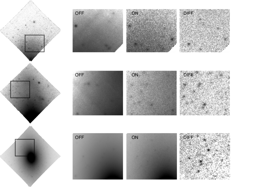
Figure 16: Examples of PN detections in NGC 1380 for pointing in the HALO (top), MIDDLE (middle), and CENTER (bottom). The zoomed regions show the off, on, and diff images and illustrate how the DELF method extracts the faint emission line objects from the bright continuum background. The resulting flat zero-background image is free from residual fixed-pattern noise.

4.1.2 Differential emission line filtering and source detection

As the first step of analysis, each cube produced by the MUSE data reduction was processed with the DELF filter to yield two diff files, one containing 13 layers of 3 co-added wavelength bins (used for source detection), and the other containing 15 layers of unbinned data (for PN measurements).

The CENTER, MIDDLE, and HALO fields were inspected visually with DS9 as described in Section 3.2. This step, which yielded 162, 73, and 29 PN candidates, respectively, is illustrated in Figure 16. In addition, Fig. 3 in Section 3.2 shows our CENTER pointing in the continuum and in two narrow layers of the stack of 13 co-added images. This figure highlights how emission line objects appear and disappear on opposite sides of the nucleus, owing to the rotation of the galaxy, and the associated Doppler shift of the PNe. The northern part of NGC 1380 is rotating towards us (blue-shifted), while the southern part is moving away from us (red-shifted). Also, in addition to the point sources, there is also a prominent feature seen near the nucleus of the galaxy which suggests the presence of an ionized disk. This disk is likely associated with the dust ring seen in the insert of (a) and participates in the rotation of the stars. We discuss this object briefly in Section 4.1.4.

The careful double-checking of diff images, e.g., Fig. 3, occasionally reveals a small mismatch in the continuum scaling factor. In this example, the mismatch is apparent to the north and south of the nucleus as white hues. This less than perfect subtraction, which is caused by rotation induced Doppler shifts of the stellar population, is irrelevant for the point source photometry which uses local estimates of the background.

We display the order of magnitude mismatch of the diff image in Figure 17. The figure shows noise histograms for ten $51\times 51$ pixel regions of the bluest unbinned diff layer in the CENTER pointing of NGC 1380. The histograms start at pixel (70,160) and then moving outward in the galaxy in increments of 10 pixels in $x$. The data show an almost perfect normal distribution of noise that increases towards the nucleus as the surface brightness of the galaxy rises. The mean varies by an amount of less than $3\times 10^{-20}$ erg cm^-2 s^-1 which is negligible in comparison with the flux of PNe near the detection limit ($\approx 300\times 10^{-20}$ erg cm^-2 s^-1).

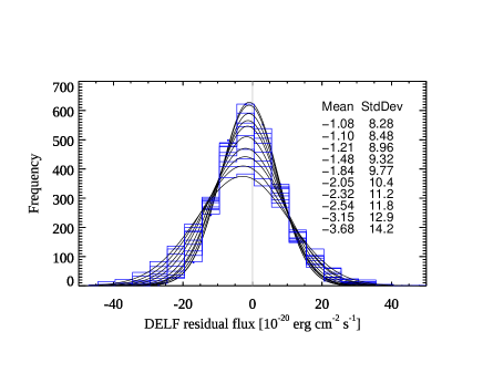
Figure 17: Residual noise in our DELF filtered frame at data cube layer 344 for the CENTER field of NGC 1380, displayed as histograms at 10 offset positions from east to west in the quadrant east of the nucleus. The Gaussian fits to each histogram are shown. Though the dispersion of the Gaussians increase as the galaxy’s surface brightness increases, the shift in the mean is negligible.

It is worth pointing out that the detection of PNe turned out to be an iterative process, involving several passes through the imaging, photometry, and spectroscopy. A detailed inspection of the images was required, which led to the discovery of as many as 15 point sources with overlapping images but different line-of-sight velocities. These blended objects were then confirmed by carefully stepping through the stack of images. A full record of detected blends is listed in the Appendix Table 5.

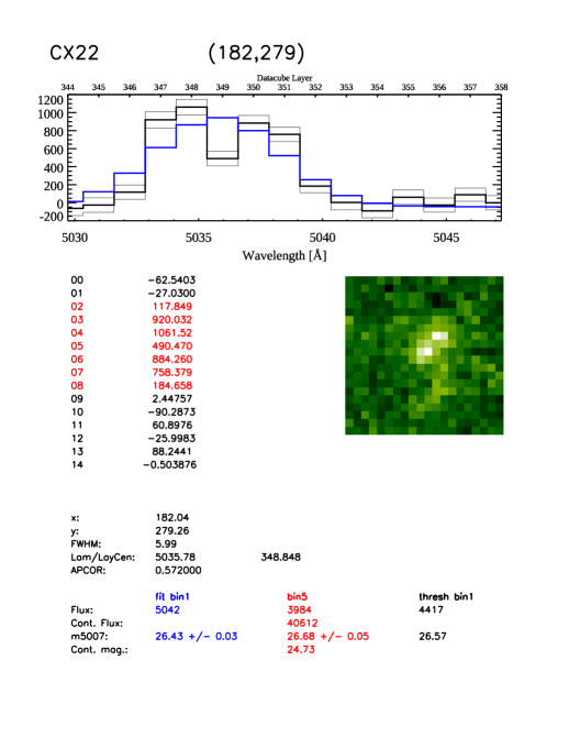
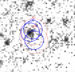
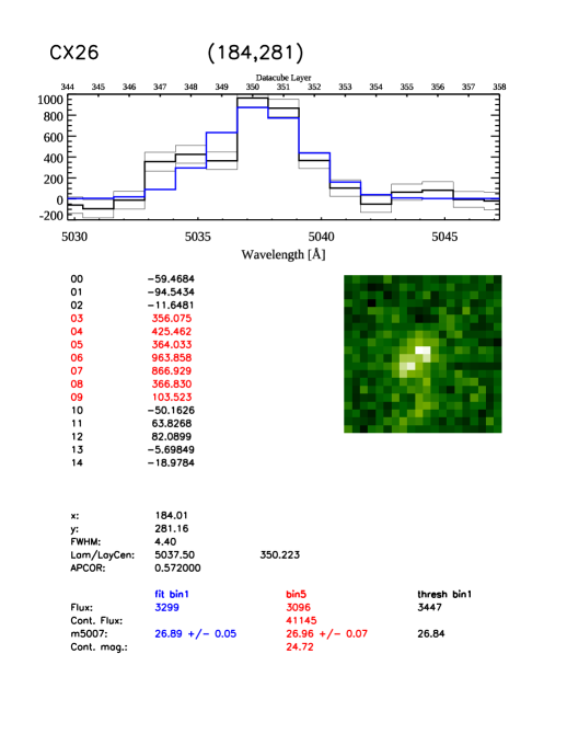
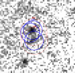
Figure 18: An example of superposed PNe in NGC 1380. Three emission line objects are located within a $1\arcsec$ radius. The top left panel shows the short spectrum for CX22 measured in a 3 pixel radius aperture; the bottom left panel shows the equivalent short spectrum for CX26, which is $0\farcs 55$ away. Note that the objects have different radial velocities. The blue curves indicate the erroneous fits before deblending. The right-hand panels show the appearance of the objects in data cube layer 348 and 350.

Figure 18 illustrates an example of such a blend. In the figure, three PN candidates are located within a region less than $1\arcsec$ in radius; such a blend would have been impossible to distinguish using the classical narrow band filter technique. Of these three sources, two were detected by Sp2020: one was classified as a PN (object Sp68 in their Table 4) and the other as a supernova remnant (object Sp70). However, a careful inspection of the top and bottom panels in Fig. 18 reveals that Sp70 has two components which are separated by $0\farcs 55$; this only becomes apparent by blinking the images centered on data cube layers 348 and 350. The short spectra extracted with a 3 pixel radius aperture for CX22 (top) and CX26 (bottom) are shown on the left hand side of Fig. 18 (explanation as in Fig. 5).

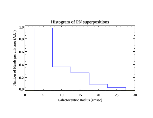
Figure 19: Histogram of PN superpositions in the central field of NGC 1380 shown as number density per unit area (in arbitrary units) versus galactocentric radius.

One can ask whether the probability of PN superpositions depends strictly on the underlying surface brightness of the galaxy. Certainly the evidence from narrow-band studies supports this hypothesis (e.g., Ciardullo et al., 1989; Jacoby et al., 1990; McMillan et al., 1993), but observations through $\sim 50$ Å wide bandpasses are not nearly as effective as MUSE at surveying the bright inner regions of galaxies. If the number density of PNe do follow the light, it would mean that the effect of blends on the PNLF is highest near the nucleus, and increases with the distance of a given galaxy. Figure 19 shows the distribution of blends as a function of galactocentric radius, which in turn is linked to the continuum surface brightness of the galaxy via de Vaucouleur’s law. The number density indeed is correlated with the surface brightness and exhibits a steep rise towards the nucleus. For radii smaller than 5 arcsec the PNLF is becoming incomplete, so no further increase is observed. The number statistics is too poor to allow for a more detailed investigation, however the trend is clear.

Measurements of the [O III] $\lambda 5007$ flux from two blended objects with a line separation of 3.75 Å cannot easily be performed with simple aperture photometry; it requires careful PSF extraction in data cubes using software similar to that used by Kamann et al. (2013) for crowded stellar fields. We have as yet not attempted to adapt this technique to the challenging problem of faint emission line objects. Instead, we employed an interactive line fitting tool that allows us to trim the contaminating spectral line with an ad hoc assumption about the true line profile for the object in the center of the aperture. This approach is not rigorously objective, but is an improvement over the poor fits that were produced before deblending (see Fig. 18).

For the current work, we identified objects with multiple emission-line components by blinking the images between the relevant data cube layers. This procedure allowed us to associate the correct components with their corresponding spatial images. Ideally one would like to automate the process, but we defer that discussion to a later paper. For now, our method of visually blinking the frames has enabled us to identify blends and improve both the photometry and line-of-sight velocity measurements.

Table 3 summarizes our final catalog of confirmed PNe in NGC 1380. In total, we identify 118 PNe in the CENTER field, 40 in the MIDDLE field, and 8 in the HALO field. For comparison, Sp2020 found 91 PNe in the CENTER field of NGC 1380, with a significant fraction (15 objects, or 16 % of their total) identified in our survey as blends (see Appendix Table 5). We also detected 70 PNe candidates near our detection limit that we classify as unconfirmed, as they are visible only in [O III] 5007 Å, i.e., they have no other confirming emission line. Of 264 point source candidates (PN and other) identified by visual inspection through 15 data cube layers, we classify only 16 (6 %) as spurious, i.e., their signal-to-noise was too low for validation. These numbers demonstrate that our differential imaging approach to PN identification is much more efficient at finding objects near the detection limit and unraveling blended point sources than techniques that work solely with the original data cubes.

More information on the classification procedure appears in Section 4.1.4 below.

Table 3: Emission line point sources detected in NGC 1380

Pointing	confirmed PN	PN candidates	SNR	spurious
Center (C)	118	31	11	2
Middle (M)	40	25	1	7
Halo (H)	8	14	0	7

4.1.3 Photometry

We performed DAOPHOT aperture photometry on the objects found in all three NGC 1380 pointings. Aperture corrections derived from stars in the field are tabulated in Appendix Table 6, and the results of the photometry are given in Appendix Table 9. A cross reference to the identifications of Sp2020 is provided in Column 2. These data allow us to perform a detailed comparison of magnitudes, signal-to-noise estimates, radial velocities, and object classifications of the two datasets.

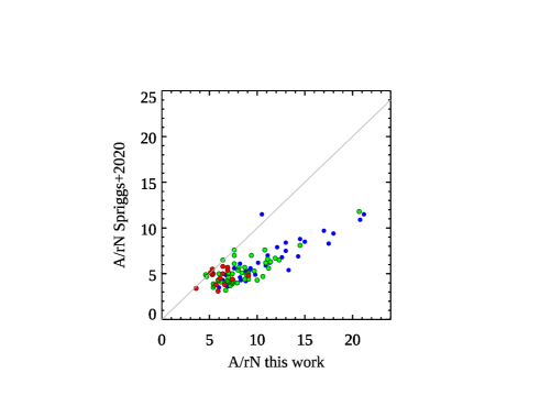
Figure 20: Signal-to-noise parameter A/rN measured by Sp2020 versus A/rN from this work. The blue points show PNe superposed on regions of relatively low galaxy surface brightness, the green points display PNe projected on areas of intermediate brightness, and the red points represent PNe located in high surface brightness regions of the galaxy. In general, the Sp2020 signal-to-noise values are $\sim 60\%$ of those measured via our DELF technique. The outlier around A/rN=11 is due to the blend of CX7+CX158 that remained unresolved (SP11) in Sp2020, cf. Appendix Table 5.

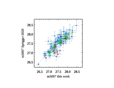
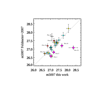
Figure 21: Comparison of our $m_{5007}$ photometry with the literature. Left: Sp2020 compared to our work. As in Fig. 20, the blue points show PNe superposed on regions of relatively low galaxy surface brightness, the green points represent PNe in regions of intermediate brightness, and the red points denote PNe located in high surface brightness areas of the galaxy. Note that the data display a systematic trend with surface brightness. Right: Fm2007 compared with our work. The color code and labels are explained in the text.

Sp2020 do not provide error estimates for their $m_{5007}$ photometry. However, we can make a meaningful comparison of the photometric uncertainties using A/rN, the ratio of the fitted emission line amplitude to the residual continuum noise for the [O III] $\lambda 5007$ emission line. Figure 20 shows our A/rN values versus those quoted by Sp2020. As our off image includes measurements of the background continuum at the position of each PN, we can track the behavior of A/rN versus the underlying galaxy surface brightness. This information is color-coded into the diagram, with blue representing objects projected onto regions of low surface brightness, and red displaying object superposed on a bright background. Regardless of PN magnitude, and except for a single outlier, the S/N ratio for the Sp2020 data is below the 1:1 line, and typically only $\sim 60\%$ of that obtained from DAOPHOT aperture photometry on DELF filtered images. This result is a direct confirmation of the expected advantage of the differential filtering approach as outlined in Section 3.2. Sp2020 excluded any objects from their analysis that fall below a threshold of A/rN = 3. In our DELF photometry, only one of those objects is close to this threshold, and only 3 are below a level of A/rN = 5. In contrast, Sp2020 reported 50 objects below this latter value, again supporting the expectation of a significant gain from our approach.

Figure 21 compares our $m_{5007}$ magnitudes to those of Sp2020 using the same color coding as in Fig. 10. Although the scatter between the measurements is larger than that expected from our internal tests (cf. Fig. 12), the relation generally follows the 1:1 line. Moreover, a closer inspection of the residuals reveals a trend in the data: objects superposed on regions of higher galaxy background surface brightness (red symbols) tend to be brighter in the Sp2020 data (mean residual of $-0.23$ mag), and the opposite is true for PN projected onto regions of lower surface brightness (blue, mean residual of $+0.14$ mag). In the absence of Sp2020 $m_{5007}$ error estimates, we have used the reciprocal of the quoted A/rN values as a proxy for their error bars in both plots, with the caveat that they are likely underestimates (see Fig. 10). Note that we confirm within the error bars the overluminous object reported by Sp2020.

More instructive is a comparison with the observations of Feldmeier et al. (2007, hereafter Fm2007), who used a narrow-band filter on the Magellan Clay telescope to identify 44 PN candidates in a 5.5 arcmin² region north of NGC 1380’s nucleus. Sp2020 compared their photometry to this dataset and reported good agreement in a relative sense for 4 matching objects in the CENTER field and 17 matches in the MIDDLE field. However, they reported that magnitudes measured by MUSE were systematically 0.45 mag fainter than those of Fm2007. Although we were unable to compare their magnitudes as they only published the photometry for the CENTER field, we decided to repeat the exercise, finding 4 matches in the CENTER, 18 matches in the MIDDLE, and 4 additional matches in the HALO. These matches include Fm2007 objects Fm1 and Fm3, which are present on both the MUSE CENTER and MIDDLE pointings, and Fm29, which is located on both the MIDDLE and HALO fields. We also discovered that thanks to the overlap of the CENTER, MIDDLE, and HALO fields, there are 9 PNe common to the CENTER and MIDDLE, and 4 objects common to the MIDDLE and HALO. Comparison of the pairs of magnitudes reveals that a satisfactory agreement is reached with an offset of -0.4 magnitudes for MIDDLE and HALO with respect to CENTER, suggesting a possible systematic error in the MUSE flux calibration, perhaps caused by non-photometric conditions. If true, this would essentially reconcile the 0.45 mag discrepancy with Fm2007 as reported by Sp2020.

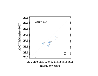
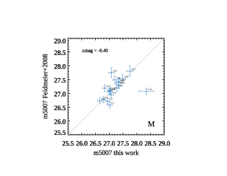
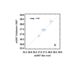
Figure 33: Comparison of the Fm2007 narrow-band filter photometry with our MUSE DELF photometry for [O III] sources in the CENTER, MIDDLE, and HALO fields of NGC 1380.

Comparison plots for each field can be found in the Appendix Figure 33, while the combined datapoints for all fields are shown in the right panel of Figure 21. The best agreement with the 1:1 line is achieved assuming a zero-point offset of $-0.1$ mag for the CENTER field and $-0.4$ mag for the MIDDLE and HALO pointings, roughly in line with the differential correction described above. However, while there is generally good agreement with the 1:1 line, a number of outliers are apparent. A careful inspection of the stack of diff images reveals that the outliers Fm1, Fm7, and Fm21 (magenta points that fall below the 1:1 line) can be explained by the contamination of PNe light by emission from diffuse gas. This effect is revealed by the velocity separation of the two components in the MUSE spectra. Fm13, which also has an anomalously bright narrow-band magnitude, is similarly identified as the blend of two overlapping point sources. The discrepancy for objects Fm19 and Fm33, (the red objects above the 1:1 line) is likely due to the velocities, as their [O III] $\lambda 5007$ emission lines (5034.48 Å  and 5032.14 Å) lie on the blue-edge of the narrow-band filter’s bandpass. Just a $\sim 20\%$ change in the filter transmission would explain the magnitude difference seen in the figure. The final discrepant object, Fm37 is located at the very edge of a MUSE data cube, and thus may have unreliable photometry.

Based on these data, we conclude that except for the above outliers, the agreement between Fm2007 and our photometry is good. In the absence of a proper calibrator, the $-0.4$ mag offset could either be due to a systematic error either in the flux calibration or the aperture correction (or both). To avoid this issue, future targeted observations must be sure to have sufficiently bright PSF stars in the field, and have flux standard exposures specifically attached to the observations.

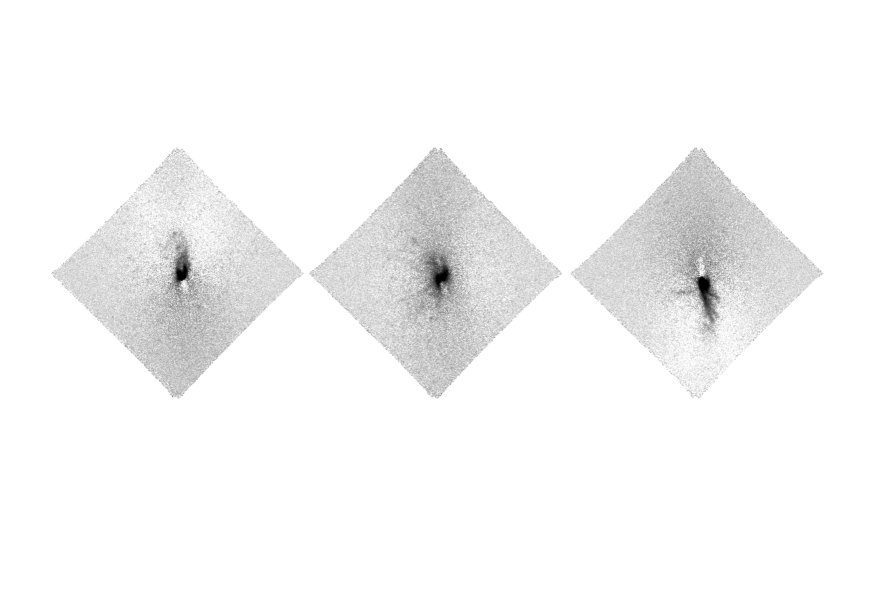
Figure 22: H$\alpha$ images and a spectrum of the ionized gas disk in the core of NGC 1380. The blue- and redshifted narrow-band images around the systemic velocity of the galaxy reveal the kinematics of the galactic plane and a complex system of filaments and knots that extend far from the principal plane of the disk. The spectrum suggests shock ionization; the shocks may also explain the nature of some of the non-PN candidates in our sample.

4.1.4 Spectroscopy

Spectra for all detected PN candidates were obtained using the entire MUSE data cube as described in Section 3.4. The main objective of this exercise was to confirm that the point-like [O III] emitters are true PNe, and to exclude interlopers such as H II regions, supernova remnants, and background galaxies. As a byproduct of this step, radial velocities were measured and tabulated for future use in kinematic analyses.

For a candidate to be classified as a PN, it was required to exhibit at least two emission lines, normally [O III] $\lambda 5007$ and [O III] $\lambda 4959$, with the latter’s flux measured to be of roughly one third of the former (Storey & Zeippen, 2000). For some faint objects near the detection limit, [O III] $\lambda 4959$ was not visible; but H$\alpha$ was. When H$\alpha$ was visible, we used the relationship for bright planetaries found by Herrmann et al. (2008, hereafter He2008) and classified the object as a PN if the flux in H$\alpha$ was smaller than the flux in [O III] $\lambda 5007$. If the [O III] $\lambda 5007$ line was the only line detected, the object was classified as a PN “candidate”. Most of these candidates should be true PNe: while single line detections could be due to background objects such as [O II] galaxies and Ly$\alpha$ emitters (LAEs), [O II] emitters would likely be detected in the continuum (Ciardullo et al., 2013), while LAEs are relatively rare. Specifically, at the depth and redshift window of the NGC 1380 data, the surface density of LAEs is roughly 0.5 objects per MUSE pointing (Herenz et al., 2019). Moreover, while the density of LAE contaminants will increase with depth, most Ly$\alpha$ emitters have line widths that are significantly wider than that expected from the [O III] line of a planetary (e.g., Trainor et al., 2015; Verhamme et al., 2018; Muzahid et al., 2020). Nevertheless, to be conservative, single-line PN candidates were not included in our PNLF analysis.

Some of the NGC 1380 PN candidates that have bright H$\alpha$ also have significant emission in the low-ionization lines of [N II] $\lambda\lambda 6548,6584$ and [S II] $\lambda\lambda 6717,6731$. This is generally the signature of shock ionization from a supernova remnant. However, NGC 1380 does not exhibit strong star formation activity, nor does it contain much cold interstellar medium, so it is unclear whether these spectral features should be attributed to SNRs. Moreover, our generalized DELF processing about H$\alpha$ reveals a $\sim 2$ kpc diameter gas disk around the galaxy’s nucleus. This disk, which has a kinematic structure similar to that seen for the PNe, has been investigated previously with the GMOS IFU (Ricci et al., 2014), and more recently with MUSE and ALMA data (Tsukui et al., 2020). As illustrated in Figure 22, the disk consists of a combination of diffuse gas and filaments with [N II]/H$\alpha$ and [S II]/H$\alpha$ line strengths indicative of shock excitation. A number of our point-like and sometimes not quite point-like objects have similar line ratios, suggesting they may actually be physically related to the disk, rather than the result of local supernova explosions. In any case, these strong [N II] and [S II] emitters are not planetary nebulae. Although the disk is interesting on its own right, its investigation is beyond the scope of this paper.

We note that the agreement between the object classifications Sp2020 and those of this work is generally good. The only differences are for SP40, which Sp2020 classified as an interloper, but we show it to have a PN-like spectrum, Sp22 (CX45), which we classify as a PN but Sp2020 lists as a supernova remnant, and Sp72 (CX115) which we consider a PN, but Sp2020 classifies as an H II region. For the rest of the Sp2020 objects our classifications agree.

4.1.5 The PNLF of NGC 1380

The left panel of Figure 23 compares the luminosity function of objects securely classified as planetary nebulae in the three fields of NGC 1380 with that derived from NGC 1380’s CENTRAL field by Sp2020. The diagram contains several features of note.

First, the central field NGC 1380 contains one PN that is “overluminous,” i.e., it appears significantly brighter than the value of $M^{*}$ predicted from the rest of the PN population. Like Sp2020, we have eliminated this object from our analysis, as its inclusion would greatly worsen the overall fit to the empirical function (decreasing its likelihood by a factor of $\sim 3\times 10^{5}$). Still, the object presents a puzzle: its spectrum looks like that of an ordinary PN, with a very high [O III]/H$\beta$ ratio, negligibly faint lines of [N II] and [S II], and an [O III]/H$\alpha$ ratio consistent with that seen in other bright planetaries (Herrmann et al., 2008). Since the object is only $\sim 0.25$ mag brighter than $M^{*}$, its apparent luminosity could be explained by a superposition of two PN within the top $\sim 0.5$ mag of the luminosity function. However, there is no evidence for two components in the shape of the [O III] $\lambda 5007$ emission line. Specifically, we used the line fitting tool pPXF (Cappellari & Emsellem, 2004; Cappellari, 2017) to measure the [O III] $\lambda 5007$ emission line more accurately than is possible by our Gaussian fitting algorithm. We find that the line profile is indistinguishable from the instrumental profile and there is no evidence of doubling. If the object is composed of two separate sources, their positions and velocities must be consistent to within roughly $0\farcs 4$ and 75 km s^-1 (one spectral bin), respectively.

Alternatively, if the overluminous source identified in the MUSE observations of NGC 1380 is a planetary nebula, it might be foreground to the galaxy. Fornax is known to have a substantial population of intracluster stars, (e.g., Spiniello et al., 2018; Spavone et al., 2020; Cantiello et al., 2020), and, since NGC 1380 sits securely in the cluster core, $0.6^{\circ}$ from the central cD galaxy NGC 1399, it is reasonable to assume some of these stars will be in the foreground. In fact, several examples of apparently overly-luminous PNe have been found in the Virgo Cluster (Jacoby et al., 1990), another system which is known to have a large population of intracluster stars (e.g., Williams et al., 2007; Longobardi et al., 2015; Mihos et al., 2017). If this is the explanation for the apparent brightness of the PN, then the object is at least $\sim 2$ Mpc in front of NGC 1380, near the turn-around radius of the cluster (Drinkwater et al., 2001). Although the presence of an intracluster $M^{*}$ PN at the extreme edge of the galaxy cluster may seem unlikely, if the PN were much closer to the galaxy, it would not be identified as an outlier in the system’s luminosity function. Thus the hypothesis cannot be ruled out.

With the current data, it is difficult to know whether either of these explanations is correct. But it is important to recognize that sources that appear too bright for the empirical function given by equation 10 are occasionally found in PN surveys of other galaxies. Also, it is interesting to note that numerical PNLF simulations (e.g., Mendez & Soffner, 1997; Valenzuela et al., 2019) do show a shallower slope at the bright end, and can produce overluminous PNe when the sample size is large. Méndez et al. (2001) have demonstrated such an effect for a sample of 535 PNe detected in NGC 4697 (see their Figures 14 and 15). Unless the PN sample contains enough objects to reliably define the shape of the luminosity function, or unless further research develops a theory for the existence of these objects, this source of contamination can lead to systematically lower PNLF distance estimates.

Fig. 23 also vividly illustrates the advantage of using DELF images rather than the normal MUSE data cubes. Our luminosity function monotonically increases to $m_{5007}\sim 27.8$ before signs of incompleteness begin to set in. The Sp2020 dataset also reaches this limit, but only in the outer regions of the CENTER field, where the surface brightness is relatively low. Identifying faint and even intermediate brightness PNe in regions of high background is difficult without first subtracting a continuum; this is reflected in the Sp2020 sample.

Finally, as the right-hand panel of Fig. 23 illustrates, despite coming from the same data, the distance we derive from our PN photometry is slightly less ($\sim 0.07$ mag) than the one obtained from the Sp2020 dataset. The cause of this difference can be inferred from Fig. 21. Because the empirical PNLF has a sharp exponential cutoff, PNLF distances depend most strongly on the observed magnitudes of the brightest few PNe in the sample. Fig. 21 demonstrates that in NGC 1380, these bright PNe lie primarily in the lower surface brightness regions of the galaxy, and for these objects, the Sp2020 magnitudes are systematically fainter than our measurements by a few hundredths of a magnitude. This translates into the offset seen in Fig. 23. The probability distributions also show the effect that our smaller measurement uncertainties and a larger sample size have on the likelihood distribution: the internal errors associated with our sample are $\sim 60\%$ smaller than those computed from the Sp2020 dataset.

Figure 23: The PNLF of NGC 1380. The left panel compares our PNLF (black points) and the most likely empirical law (solid curve) with Spriggs et al. (2020) luminosity function (red points) and its mostly likely fit (dotted curve). The open points show the one overluminous object (which is not fit) and PNe beyond the completeness limit. The right panel displays the likelihood of the solution versus the distance modulus. These likelihoods assume $M^{*}=-4.53$ and a foreground reddening of $A_{V}=0.046$, but do not include systematic errors associated with the frames’ aperture corrections, flux calibrations, and foreground reddening.

The maximum likelihood solutions shown in Fig. 23 bring up an interesting issue for future PNLF measurements. If we assume a foreground reddening of $E(B-V)=0.046$ (Schlafly & Finkbeiner, 2011) and an absolute value for $M^{*}=-4.53$ (Ciardullo, 2013), then the most-likely distance modulus to NGC 1380 is $(m-M)_{0}=31.10^{+0.04}_{-0.05}$ (16.6 Mpc), with additional systematic uncertainties associated with the errors on the frames’ aperture corrections, flux calibration, and the amount of foreground reddening. For comparison, the Surface Brightness Fluctuation method generally produces values between 31.20 and 31.60 (e.g., Tonry et al., 2001; Blakeslee et al., 2009, 2010). This offset of $\sim 0.3$ mag is not unexpected, and may be explained by a very small amount of internal reddening in the Cepheid galaxies used for calibration. As has been pointed out by Ciardullo et al. (1993) and again by Ciardullo et al. (2002a), both the PNLF and SBF methods use relatively late-type galaxies to define the zero points of their distance scales. However, any systematic difference between the amount of internal reddening present in these galaxies and that within the early-type systems targeted by the methods will lead to the SBF scale being overestimated and the PNLF scale being underestimated, with $\Delta\mu\sim 7\Delta E(B-V)$, i.e., $\Delta E(B-V)\sim 0.04$.

Alternatively, we can compare our distance modulus to those derived from Cepheid and TRGB measurements of other cluster galaxies. NGC 1326A and 1365 are both projected within $\sim 1$ Mpc of the Fornax central cD galaxy (NGC 1399), have radial velocities consistent with cluster membership, and have been surveyed for Cepheids by the Hubble Space Telescope. Their mean Cepheid-based distance modulus of $(m-M)_{0}=31.10$ (Freedman et al., 2001) is identical to our measurement. On the other hand, the TRGB distance to NGC 1365 is $0.19$ mag more distant than our value (Jang et al., 2018). Moreover, if NGC 1425 (a galaxy projected $5.6^{\circ}$ away on the sky) is also considered to be part of Fornax, then its Cepheid distance ($(m-M)_{0}=31.60$; Freedman et al., 2001), when averaged with those of NGC 1326A and 1365, makes the cluster’s mean Cepheid distance consistent with that of the TRGB. So it is possible that the PNLF distances are still biased slightly towards smaller values.

4.2 Benchmark galaxy: NGC 628

NGC 628 (M74) is a large SA(s)c spiral galaxy that has hosted two Type II (SN2003gd and SN2013ej) and one Type Ic (SN2002ap) supernovae in the past two decades. The galaxy is the brightest and largest member of its group, extending over $12\arcmin$ on the sky, and is viewed almost face-on, with an inclination angle of only $6.5^{\circ}$ (Kamphuis & Briggs, 1992). Because the galaxy is so face-on, the distribution of PN velocities about the galaxy’s systemic value of $v_{\rm rad}=657$ km s^-1 (Lu et al., 1993) is quite narrow, ranging from $\sigma_{v}\sim 50$ km s^-1 in the central arcmin to less than 15 km s^-1 $\sim 4$ disk scale lengths away (Herrmann & Ciardullo, 2009a).

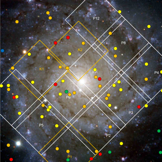
Figure 24: MUSE observations of NGC 628, with the pointings of Kreckel et al. (programme 094.C-0623, labeled K1 and K2) and Blanc et al. (programme 098.C-0484, labeled P1 through P12) outlined as orange and white squares. A PNLF was determined by Kr2017 from PNe in K1, K2, and P1. PNe detected with OPTIC at the WIYN telescope by He2008 are overplotted as circles as an adaptation from their Fig. 2. The color code in red, orange, yellow, and green represents objects in the top 0.5, 1.0, 1.5, and 2.0 mag of the PNLF. Orientation: North up, East to the left. Background image credit: ESO PESSTO Survey (Smartt et al., 2015).

TRGB measurements place NGC 628 between 9.5 to 10.7 Mpc away, while estimates from the Type II SN 2003gd and the galaxy’s brightest supergiants generally give values between 7 and 10 Mpc (see McQuinn et al., 2017, and references therein). Two PNLF distances also exist in the literature, but they are discrepant by $\sim 1.5\sigma$: while the interference-filter based photometry of He2008 gives 8.6 Mpc, the MUSE analysis by Kr2017 yields 9.6 Mpc. The latter authors argue that their larger distance is a consequence of MUSE’s ability to exclude compact SNRs from the PN sample. However, since Davis et al. (2018) has argued that supernova remnants can rarely affect a PNLF distance measurement, it is worth revisiting the robustness of their measurement.

Figure 24 displays an image of NGC 628, along with the locations of the PNe found by He2008 and the 12 pointings recorded in the MUSE archive. The analysis by Kr2017 used three of these pointings, yielding a total of 63 PNe. However, by analyzing the PNe found in all 12 pointings, we can make a detailed photometric comparison with 51 of the PNe measured by He2008. Although the full complement of 12 fields was obtained for another science case, and thus were not all taken under photometric conditions, the overlap with He2008 can be used for bootstrapping the different MUSE exposures to a common photometric zero point. Moreover, one of the fields (P3) was observed twice at different epochs, and under different observing conditions. The data set is therefore attractive for assessing the robustness of our analysis technique, as it allows us to perform both internal and external consistency checks.

4.2.1 Data, source detection, and classification

       

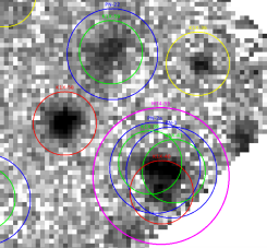
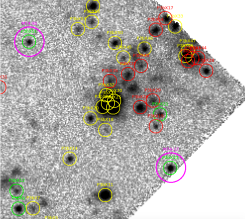
Figure 25: Source confusion due to crowding. Left: M74-33 (magenta circle) was resolved by Kr2017 into two objects PN1 and PN2a (blue). Our [O III] map shows that there are actually three sources in the blend, two of which are PNe (green), the third one classified a SNR (red). Middle: M74-11 from He2008 in field P6 is resolved into two PNe, and is one of the outliers in the left panel of Fig. 26. Right: the outliers below the 1:1 line in Fig. 27 in field P3 are identified as H II regions (yellow) and SNRs (red) in a heavily crowded region of the galaxy.

Except for the data reduction, where we immediately used the fully reduced data cubes as downloaded from the ESO archive, the basic steps for analysis were identical to the ones described for NGC 1380 in Section 4.1. Source detection was facilitated on the one hand by the fact that the narrow velocity dispersion perpendicular to the disk reduced the number of data cube layers that needed to be inspected. However, the large number of point-like H II regions and SNRs complicated the issue. We were able to efficiently identify a promising sample of PNe by supplementing the detections of the DAOPHOT FIND algorithm with visual inspection of the data cubes. We then performed photometry and spectroscopy on the source list to measure emission line strengths and classify the objects via their line ratios (see Table 4).

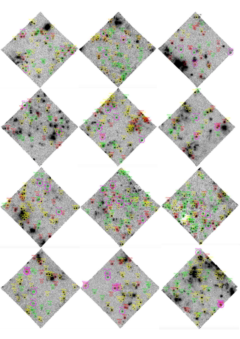
Figure 35: All 12 MUSE pointings available for NGC 628 shown as images in [O III]  $\lambda 5007$, coadded from three datacube layers around the [O III] wavelength, Doppler-shifted to the systemic velocity of the galaxy. Green circles: PN candidates, yellow: H II regions, red: SNR. Magenta circles indicate objects in common with He2008. We have detected a total of 244 PN candidates, 295 H II regions, and 160 SNR.

[O III] maps for all fields are presented in the Appendix Figure 35. As was found in the analysis of NGC 1380, careful inspection of the images was needed to identify blends. Figure 25 shows a few examples of multiplicity, some of which have escaped detection in previous studies. Such cases can explain the [O III] magnitude differences between our MUSE data and the measurements of other studies (see Section 4.2.2 below).

Table 4: Emission line point sources detected in NGC 628

Pointing	Confirmed PNe	Candidate PNe	SNRs	H II	seeing (1)	weather (2)	$\Delta$m (3)
K1	16	3	10	28	$0\farcs 77$	clear	$+0.10$
K2	31	5	20	18	$0\farcs 83$	clear	$-0.20$
P1	11	…	16	7	$0\farcs 76$	clear	$-0.10$
P2	9	3	12	11	$1\farcs 14$	clouds	$-0.03$
P3a	13	3	19	39	$1\farcs 49$	clear	$-0.40$
P3b	13	3	19	39	$0\farcs 95$	clouds	$-0.40$
P4	11	…	9	16	$1\farcs 08$	clear	$-0.11$
P5	10	…	15	35	$1\farcs 05$	clouds	$-0.20$
P6	31	5	17	21	$0\farcs 69$	clouds	$-0.00$
P7	38	12	17	37	$0\farcs 70$	clouds	$-0.35$
P8	13	2	6	28	$0\farcs 82$	clouds !	$-0.80$
P9	6	3	13	23	$0\farcs 96$	clouds !	$-0.95$
P12	15	4	6	32	$0\farcs 75$	clouds !	$-0.14$

Note. — (1) Seeing FWHM (ESO Archive information), (2) Retrieved from ESO Archive: “clouds”: some clouds registered during the night,“clouds !”: clouds passing during an exposure, (3) zero-point offset used to match the He2008 photometry.

4.2.2 Photometry

[O III] measurements were performed in the standard way as described above. However, our photometry was limited by two issues. The first was weather: according to the ESO archive, most of the MUSE observations of NGC 628 were affected by clouds. More serious was the lack of point sources in the field. Unlike NGC 1380, we found it difficult to identify foreground stars suitable for aperture correction measurements. As shown in in Fig. 6, the FWHM vs. wavelength relation for NGC 1380 was well-behaved, and followed the expectations of atmospheric turbulence. However, in NGC  628, there were significant differences between the point sources candidates of each field, and for some objects, we even measured the FWHM to increase with wavelength. Such an effect could conceivably be produced if the target objects were not actually stars, but globular clusters with a large population of blue stragglers concentrated in the core. Attempts to create a model PSF by stacking PN images also proved problematic, as the result was sensitive to the surface brightness of the galaxy’s ubiquitous diffuse background emission. The aperture corrections, which are the dominant source of uncertainty in our photometry, and the catalogue of PN candidates are presented in the Appendix, Tables 7 and 10, respectively.

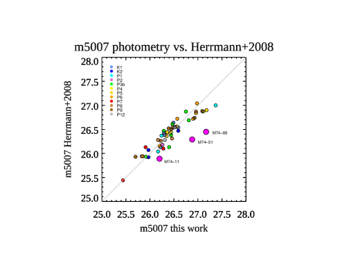
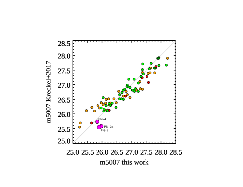
Figure 26: Comparison of our $m_{5007}$ photometry in NGC 628 with PN photometry from He2008 (left) and Kr2017 (right). The color-coding on the left represents different MUSE pointings; that on the right illustrates that different classes of objects, with PNe in green, H II regions in orange, and SNRs in red. The large magenta circles are indicating object blends (see text).

Figure 27: Comparison of photometry in field P3 from two MUSE observing runs with very different image quality (P3a: $1\farcs 49$, July 25, 2017; P3b: $0\farcs 95$, November 13, 2017). PNe are in green, H II regions in orange, and SNRs in red. For the interpretation of outliers (magenta), see text.

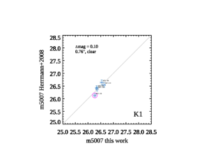
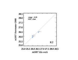
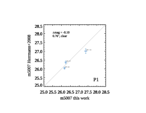
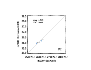
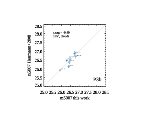
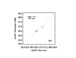
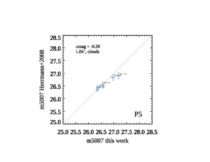
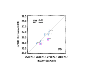
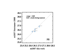
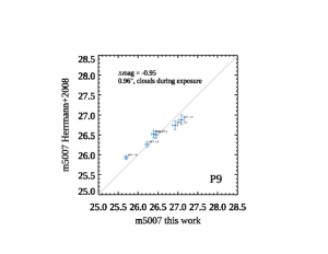
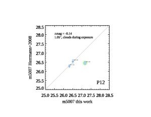
Figure 36: Comparison of $m_{5007}$ photometry in all 12 MUSE pointings in NGC 628 with the narrow-band filter photometry of He2008. Magenta circles indicate outliers due to blending of multiple sources. The green circle for M75-69 in field P12 indicates an outlier due to coverage in only 1 out of the 3 dithered sub-exposures. Seeing and atmospheric conditions are indicated for each exposure. To compensate for non-photometric conditions, the zeropoint of the MUSE photometry has been shifted to achieve the best fit with the comparison data.

Because of these difficulties, we used the He2008 PN photometry as the flux standard system for our measurements. A comparison of our corrected $m_{5007}$ values with the He2008 data is documented in the Appendix Figure 36. The agreement between the two datasets is generally good, except for the outliers caused by blending. A collapsed version of measurements for all 51 objects in common with He2008 is shown in the left panel of Figure 26. For PNe brighter than $m_{5007}=27.0$ the residuals display a standard deviation of 0.12 mag, which is in reasonable agreement with the uncertainties quoted by He2008 ($\pm 0.058$ mag at $m_{5007}=26.0$ and $\pm 0.135$ mag at $m_{5007}=27.0$).

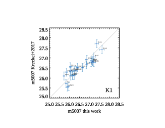
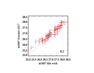
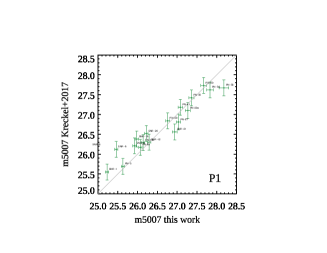
Figure 34: Comparison of our $m_{5007}$ DELF photometry with the MUSE measurements of Kr2017 for fields K1, K2, and P1 in NGC 628.

The right panel of Fig. 26 adjusts our photometry in fields K1, K2, and P2 by $-0.2$ mag, and compares the measurements with those of Kr2017. The plot is broken down by object classes, with H II regions coded in orange, SNRs in red, and PNe in green. The magenta points at the bright end of the distribution are objects where undetected source confusion affected the Kr2017 photometry. The standard deviation for the PN measurements is 0.21 mag, in agreement with the Kr2017 error estimates. See also Fig. 34 in the Appendix for comparison plots per field K1, K2, and P1.

Fig. 27 shows a comparison of the $m_{5007}$ magnitudes for all emission line point sources (PNe, H II regions, SNRs) obtained in field P3 at two different observing epochs under different observing conditions. While the He2008 photometry had a completeness limit of $m_{5007}=26.5$, the MUSE data extends roughly 2.5 magnitudes fainter, with an internal dispersion of 0.15 mag and a mean residual of 0.004 mag for PNe brighter than 28.0 mag (excluding outliers). The bright outliers (magenta) between $25<m_{5007}<27$ are H II regions and SNRs in crowded regions that suffer from blending (several examples are shown in the right panel of Fig. 25). For this internal consistency check, no zero point shift has been applied.

4.2.3 The PNLF of NGC 628

The left-hand panel of Figure 28 displays the bright-end of the planetary nebula luminosity function for NGC 628. Although our PN observations extend all the way to $m_{5007}\sim 29$, we only use the top $\sim 1.5$ mag of the function in our fit. This is due to the fact that, in star-forming populations, the PNLF is not monotonic: instead of exponentially increasing at faint magnitudes, the function exhibits a distinctive dip 2 to 4 magnitudes below $M^{*}$. This feature, first identified by Jacoby & De Marco (2002), occurs in PN populations that are dominated by objects with intermediate and high-mass cores and is discussed in Ciardullo (2010). Since equation 10 does not attempt to model this downturn, we truncate our fit at $m_{5007}\sim 26.9$, and do not use the faintest $\sim 55\%$ of our sample.

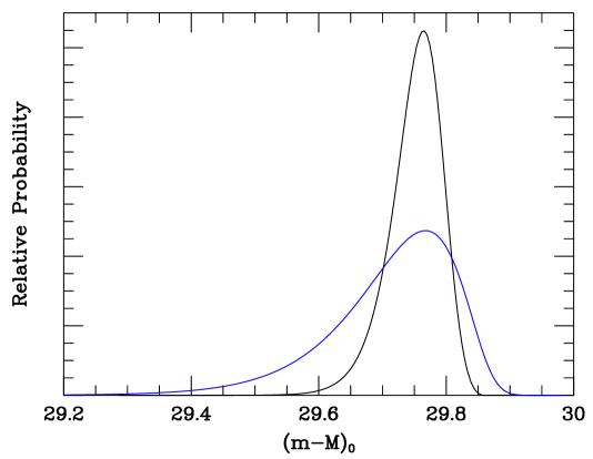
Figure 28: The PNLF of NGC 628. Left: The observed PN luminosity function binned into 0.2 mag intervals. The solid curve is the empirical function of equation 10 shifted by the most likely apparent distance modulus; the dashed curve is the best-fit solution if the brightest PN is omitted from the sample. Right: The relative likelihood versus distance modulus curve for our PN sample (black curve) and Kr2017 sample (blue curve). Both datasets produce the same most-likely distance, but our larger sample size results in a much smaller uncertainty.

The right-hand panel of Fig. 28 displays the uncertainty in our distance modulus. Assuming a foreground galactic extinction $E(B-V)=0.062$ (Schlafly & Finkbeiner, 2011), our most-likely distance modulus is $(m-M)_{0}=29.76^{+0.03}_{-0.05}$ (or 8.95 Mpc), where the uncertainties represent only the statistical errors of the fit. When analyzed using our maximum likelihood technique and using the same value of $M^{*}$, the Kr2017 data give $(m-M)_{0}=29.76^{+0.12}_{-0.05}$, while the PNe of He2008 yield $(m-M)_{0}=29.73^{+0.06}_{-0.07}$. However, we should point out that this apparent consistency hides a potentially important issue: the brightest PN in our sample (P7-38), though not strictly overluminous, is 0.11 mag brighter than the next brightest source. There is no reason to exclude the object from the analysis, as our best-fit to equation 10 is clearly acceptable. However, if do we exclude the object, the best-fit solution becomes $\sim 90$ times more likely, and the galaxy’s distance increases to $29.87^{+0.03}_{-0.05}$.

This issue points out an important limitation of using planetary nebulae for distance determinations. To determine a robust distance using the PNLF, one cannot depend solely on the magnitude of the most luminous PN in a galaxy. Instead, one has to define the shape of the brightest $\sim 1$ mag of the PN luminosity function. Unfortunately, PNe in this critical magnitude range are rare: the specific PN densities given by Ciardullo et al. (2005), coupled with the galaxy bolometric corrections computed by Buzzoni et al. (2006) imply that an $M_{V}=-19$ galaxy will only contain $\sim 20$ PNe in the magnitude range of interest. In the era of precision cosmology, this number is not sufficiently constraining, as the distance may be susceptible to contamination by bright interlopers, or it may be underpopulated, leading to a large uncertainty in distance. As Fig. 28 illustrates, a minimum of $\sim 50$ objects are needed for a robust measurement of the PNLF shape. PN surveys must therefore sample at least $M_{V}\sim-20$ of a galaxy’s luminosity.

4.3 Benchmark galaxy: NGC 474

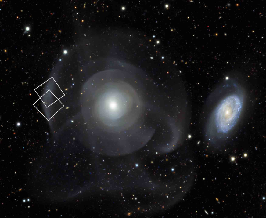
Figure 29: MUSE observations in NGC 474. This $12^{\prime}\times 10^{\prime}$ image (with north up and east to the left) shows the Arp 227 group with the dominating ring galaxy NGC 474 in the center and the gas rich group member NGC 470 to the west. Two MUSE pointings centered on an outer shell of the galaxy are illustrated; each represent a 5.1 hour exposure by Fe2020. Image credit: DES/DOE/Fermilab/NCSA & CTIO/NOIRLab/NSF/AURA

NGC 474 is classified as a lenticular galaxy (Type SA0(s) in the RC3 catalogue; de Vaucouleurs et al., 1991) and is well known for its tidal tails and shell-like features. IFU observations with SAURON have measured the system’s radial velocity to be $2315\pm 5$ km s^-1 (Cappellari et al., 2011), placing the object at a Hubble distance of roughly 32 Mpc. Tully-Fisher distances in the range of 15.3 to 35.0 Mpc were obtained by Bottinelli et al. (1984), while more recent SBF measurements suggest a distance of between 30 and 33 Mpc (Cantiello et al., 2007). Figure 29 show the galaxy’s spectacular system of rings and tidal arms, which are presumably a result of a merger event. Fensch et al. (2020), henceforth Fe2020, obtained deep MUSE exposures in the outer ring with the goal of studying the star formation history and metallicity of the structure. Their reported discovery of 8 PN candidates makes the object an interesting benchmark case, as it allows us to test our technique in a galaxy whose distance is well beyond the limit of classical PNLF measurements.

4.3.1 Data, source detection, classification, photometry

The data retrieval and emission-line analysis proceeded as above. The fully reduced data product as available in the ESO archive consists of a single cube, where two datasets of total exposure time 5.1 hours were merged into one. Therefore, in the overlapping region of the two fields shown in Fig. 29, the total exposure time was more than 10 hours. As can be seen in the off-band image displayed in Figure 30a, the faint surface brightness in this ring region is strongly modulated by the residual flatfield pattern discussed in Section 3.2. This systematic error has completely vanished after DELF processing, yielding the diff images shown in Fig. 30b. The exquisite quality and depth of this region allowed us to easily confirm the 8 objects found by Fe2020 and identify 7 additional PNe candidates. (Since three of these new objects are single-line detections, we classify them as possible PNe and do not use them in our analysis.) Thus, the observations yielded 12 likely PNe with [O III] magnitudes in the range $28.5\lesssim m_{5007}\lesssim 30.2$. Serendipitously, our PN search also discovered two $z=4.551$ Ly$\alpha$ emitters, one of which overlaps with PN8. The region containing PN8 and a Ly$\alpha$ emitter is shown in the inset of Fig. 30.

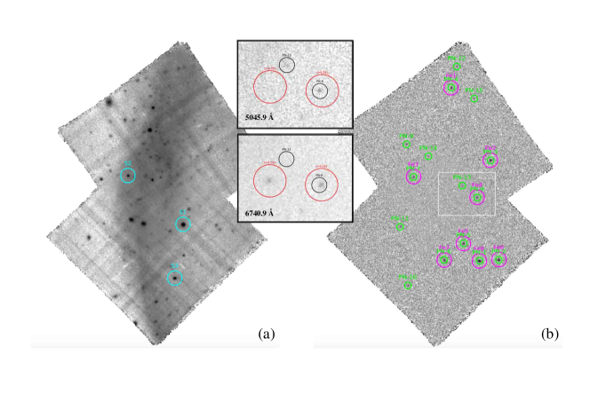
Figure 30: Off and diff images of NGC 474, with north up and east to the left. (a) Continuum (off-band) image, with the three point sources used for our aperture correction marked in cyan. (b) The diff image at radial velocity 2267 km s^-1 (5044.69 Å), summed over 3 layers of the data cube. The PN candidates are marked as green circles. The objects detected by Fe2020 are marked in magenta. The inserts highlight the chance alignment of PN8 with a background galaxy (see also Fig. 8).

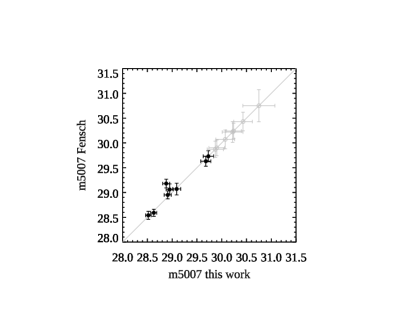
Figure 31: Comparison of our $m_{5007}$ photometry with that of Fe2020. The symbols in grey are intended to illustrate the depth of our photometry, but are not meaningful for this comparison).

As was our experience with NGC 1380, the selection of point sources for measuring the cube’s PSF and aperture correction was non-trivial, as many of the brighter objects are either globular clusters or background galaxies. Using three objects marked in Fig. 30a, we measured [O III] FWHM values of $0\farcs 76$ in the combined field, and $0\farcs 78$ in the southern field. Precision photometry would require us to accurately measure the PSF in each subfield separately, but for the sake of simplicity in this experiment, we have neglected the (very small) difference in image quality. The adopted aperture corrections and our catalogue of PN candidates are found in the Appendix, Tables 8 and 11, respectively.

To compare our photometry with the literature, we needed to convert the absolute $M_{5007}$ values listed by Fe2020 to apparent $m_{5007}$ magnitudes. However, with their assumed distance modulus of $(m-M)_{0}=32.45$, the comparison resulted in an offset of 0.5 mag. With a choice of $(m-M)_{0}=32.95$, and a foreground extinction of 0.1 mag (Schlafly & Finkbeiner, 2011), we obtain excellent agreement as shown in Figure 31. The single outlier at $m_{5007}=28.9$ is probably due to the presence of three continuum point sources very close to the centroid of our PN4 (PN1 in the nomenclature of Fe2020).

Note that the grey plot symbols, although self-referenced to our own magnitudes, are only intended to illustrate the range of photometry possible with deep MUSE exposures. These data, which should be compared with the simulations described in Section 3.6.2 and shown in Fig. 12, demonstrate that a $\sim 10$ hr exposure with MUSE can reach [O III] $\lambda 5007$ magnitudes as faint as $m_{5007}\sim 31$. Moreover, with the MUSE image quality that is currently being achieved with adaptive optics this limit can be improved significantly. For example, in the MUSE Extremely Deep Field combined data cube, an image quality of $0\farcs 6$ FWHM at 4700 Å has been achieved over a total exposure time of 140 hours (Bacon et al., 2021). Thus, it should be possible to push PN detections well past the distance of NGC 474.

4.3.2 The PNLF of NGC 474

Figure 32: The PNLF of NGC 474. On the left is the observed PNLF with our best-fit empirical law shown as a solid line; a completeness limit of $m_{5007}=29.1$ has been assumed. The right hand panel plots the relative likelihood versus distance modulus. The asymmetrical nature of the probability curve is typical for PNLF measurements with a limited number of objects: it is always possible to bring the galaxy closer, as that just moves the PNe further down the luminosity function. But since equation 10 has a sharp cutoff at $M^{*}$, there is a hard upper limit to how far away the galaxy can be.

Figure 32 illustrates our PN luminosity function for NGC 474. The PN sample is small, not because of any issue with the quality or depth of the MUSE observations, but because the amount of galaxy luminosity encompassed by the survey fields is small. As a result, the data cannot be used to obtain a robust measure of the distance to the galaxy. Nevertheless, if we assume that all the PNe are drawn from the empirical function of equation 10, we can perform a maximum-likelihood analysis on the data and obtain an estimate of the galaxy’s distance. We adopt a 90% completeness magnitude limit of $m_{5007}=29.1$; this ad hoc assumption could be improved by running a series of artificial star experiments on the data cube, but is sufficient for our purpose. If we then assume a foreground $E(B-V)=0.03$ (Schlafly & Finkbeiner, 2011), the most-likely distance modulus obtained from the PNe is $(m-M)_{0}=32.86^{+0.08}_{-0.25}$, or $37.4^{+1.5}_{-4.0}$ Mpc. Again, these error bars only represent the formal uncertainties of the fits. Systematic errors associated with the aperture correction, foreground reddening determination, and assumed value of $M^{*}$ are not included in the calculation. This distance is fully consistent with that obtained from the SBF analysis (Cantiello et al., 2007).

5 Discussion

5.1 Accuracy of MUSE photometry

Our goal is to utilize the unique capabilities of MUSE with adaptive optics to make the PNLF a precision distance determination tool for cosmology. To prove this claim, we must first assess the uncertainties involved in this technique, both random and systematic. As the PNLF is a photometric standard candle, one of these uncertainties is the error in the photometry. In Sections 3.6 and 4 we have demonstrated using simulations and through the analysis of archival data that it is possible to obtain an internal photometric accuracy of 0.04 mag for the brightest magnitude bins of the PNLF. Moreover, tests indicate that our photometry is valid down to at least $m_{5007}=30$, with formal error estimates that are empirically validated by the statistics of mock data.

Our archival benchmark tests on NGC 1380 and NGC 628 have shown that accurate PN photometry is achievable with exposure times of less than an hour under reasonably good seeing conditions ($0\farcs 8$) out to distances of $\sim 20$ Mpc. The experiment with archival data for NGC 474 suggests that the same level of photometric accuracy can be reached with exposure times of 10 hours out to a distance of almost 40 Mpc. It is therefore safe to assume that, with the image quality that can be expected from MUSE+GLAO observations, these numbers are conservative estimates. By observing $\sim 50$ PNe in the top $\sim 1$ mag of the PNLF in one or two AO-assisted exposures, MUSE should be able to obtain relative distances that are accurate to $\Delta\mu\approx 0.05$ mag.

Two major contributions to the total error budget come from the calibration of the photometric zeropoint, namely the uncertainties in a frame’s aperture correction and flux calibration, and our imperfect knowledge of the foreground extinction. The latter issue is one that affects most distance indicators and has improved with time as our measurements of the long-wavelength emission of dust has improved (e.g., Aniano et al., 2020). Future work may also reveal ways to use the MUSE datacube to independently estimate E(B-V) from a stellar population analysis of the underlying host galaxy (Zahid et al., 2017; Li et al., 2020, 2021).

The former problem is more serious, especially for a complex, limited-field instrument such as MUSE. We were able to cope with problems with the photometric zero point in our analysis: since some of the archival data used for this study were taken under non-photometric conditions, frame-to-frame offsets in the calibration were apparent at the level of $\pm 0.1$ mag. Fortunately, as we will show in Section 5.3, there are a number of observing strategies that can reduce this error to roughly a couple of percent.

5.2 Limitations of the PNLF

The robustness of PNLF distances ultimately comes down to two questions: what is the precise shape of the bright-end of the PNLF, and does this shape change with stellar population? At this time, theory cannot answer these questions. The value of $M^{*}$ and the observed circumstellar extinction around $M^{*}$ planetaries imply that the central stars that power [O III]-bright PNe have intrinsic luminosities of over $\sim 11,000\ L_{\odot}$ and central star masses greater than $0.66M_{\odot}$(Herrmann & Ciardullo, 2009b; Davis et al., 2018). Despite over 30 years of research, there is still no theory to explain the existence of these objects in Population II systems such as elliptical galaxies. Thus our understanding of the behavior of the PNLF’s bright-end cutoff must be achieved empirically, via the analysis of a broad range of observations (e.g., Bhattacharya et al. (2021)).

Based on the magnitude distribution of planetary nebulae in M31’s bulge, Ciardullo et al. (1989) originally proposed truncating the power-law distribution modeled by Henize & Westerlund (1963) with the expression given by Equation 10. This law, which is similar to the results of numerical models that use ad hoc assumptions for the core masses of [O III]-bright PN central stars (Jacoby, 1989; Mendez et al., 1993; Mendez & Soffner, 1997; Valenzuela et al., 2019), has proved reasonably reliable and repeatable. However, as discussed in Section 4.1, “overluminous” [O III] sources are occasionally found in PN surveys. Because most of the PNLF observations to date have been performed using narrow-band filters and have very little (if any) spectroscopic follow-up, it has been difficult to determine the nature of these sources. Are they true PNe or unrelated objects such as supernova remnants, compact H II regions, blends of multiple objects, or background galaxies? If the objects are PNe and if they are indeed located within the targeted galaxy (as opposed to a foreground intergalactic object), then the empirical form of the PNLF will have to be modified in order for the PNLF to achieve the precision necessary to address questions of cosmology.

MUSE provides the information needed to understand the nature of some overluminous sources. Certainly, at least some of the overluminous [O III] sources have spectra that are indistinguishable from PNe (e.g., Ciardullo et al., 2002b, and the MUSE observations of NGC 1380 described in this paper). But deep, narrow-band PN surveys also have their share of contaminants (e.g., Kudritzki et al., 2000; Durrell et al., 2003; Longobardi et al., 2013). As shown above, MUSE spectra are very efficient at identifying the interlopers in PN surveys. Moreover, by comparing PN luminosity functions inside and outside of clusters, MUSE will also be able quantify the importance of intracluster PNe in PNLF analyses.

A related parameter that is key to using the PNLF for cosmology is the exact value of $M^{*}$ and its dependence on the host galaxy population. Unlike Cepheids or the TRGB methods, there is no immediate prospect for a Galactic calibration of the PNLF. Thus, the PNLF is a secondary standard candle, and its distances will always carry some error originating with the distance measurements to nearby galaxies. At present, the uncertainty in $M^{*}$ is roughly $\sim 0.04$ mag (Ciardullo, 2013), though this can be improved via MUSE observations of additional Cepheid and TRGB galaxies.

Ideally, we wish to develop a more thorough theoretical basis for the PNLF to improve our application of the PNLF and our confidence in the results. We are not at that point yet.

5.3 Future application for the PNLF using MUSE

One of the most important parameters for deriving accurate PNLF distances will be the image quality (i.e., the seeing). As noted by our simulations in Section 3.6, the difference between $1\farcs 0$ and $0\farcs 6$ is dramatic, both for extending the reach of the PNLF in distance and for enabling PN identification in high surface brightness regions of a galaxy. The recent MXDF project (Bacon et al., 2021) has demonstrated that an image quality of $0\farcs 6$ at a wavelength of 5000 Å can be consistently obtained when using the GLAO system at UT4 of the VLT. Future PNLF observations will clearly benefit from GLAO.

Many of the observations in the MUSE archive are not optimized for precision spectrophotometry. For example, one potential source of error is the flux calibration. Typical MUSE observations include flux standards taken at the beginning and end of each night. Additional flux calibrations taken before and after PNLF exposures (with as similar an airmass as possible) can reduce any uncertainties incurred from subtle changes of atmospheric transmission over the course of a night.

A related and serious issue is the need to derive a frame’s aperture correction in order to place relative photometric measurements onto an absolute magnitude scale. The pre-selection of fields that contain sufficiently bright point sources will ensure that each frame contains suitable PSF standards. But care must be taken at this step, since globular clusters can often be mistaken for point sources; in general, the better the angular resolution, the easier it is to choose point sources. Once chosen, the PSF stars can be analyzed by MUSE, but, if they are sufficiently bright, they can also be calibrated with spectrophotometric measurements from other telescopes. Such observations need only be taken at a wavelength near 5007 Å, and, because the aperture correction is a very slow function of wavelength the observing bandpass can be fairly broad, perhaps 250 Å wide. Finally, an attractive opportunity to model the PSF for MUSE GLAO observations has been put forward by Fusco et al. (2020). The muse-psfrec software can be used to reconstruct the PSF from the real-time adaptive optics telemetry information recorded by the MUSE adaptive optics system GALACSI.

Another observing strategy that can assist PNLF measurements is the selection of fields having relatively low surface brightnesses. The high surface brightness regions of a galaxy naturally have more planetary nebulae, as PNe are excellent tracers of the light, and vice versa. However, even with the effectively narrow bandpass from MUSE, the dominant noise source in a PNLF observation is the brightness of the underlying galaxy background plus night sky. The location of a MUSE pointing must be optimized to maximize the number of PNe expected to be found while minimizing the number of fields necessary to obtain a statistically useful PN sample, i.e., $\gtrsim$50 PNe within the brightest mag of the PNLF.

A careful selection of galaxies is also needed for several reasons. First, the earlier criticisms of biases in PNLF distances beyond $\sim$15 Mpc needs to be better understood. Is this a bias arising from pushing into a regime beyond the data quality? Is it due to the misclassification of other emission-line objects as PNe? Or is the error intrinsic to the PNLF itself, perhaps due to the failure of the empirical form of the PNLF to account of “overluminous” objects, intracluster stars, and object blends? MUSE observations in a few fields of suspect galaxies from previous PNLF studies will help resolve the source of a bias, or perhaps demonstrate that there is no bias.

Galaxy selection is also critical for extending the PNLF distances to $\sim 50$ Mpc. The target galaxies should ideally be well-structured early type systems to minimize confusion with H II regions and SNRs, but also offer a sample of Type Ia supernovae to be calibrated. Since these galaxies are beyond the reach of the TRGB and do not have Cepheid variables, they would immediately contribute to the SN Ia calibration.

Finally, it is worth noting the development of BlueMUSE (Richard et al., 2019). With a larger field-of-view of 2 arcmin², a $\tilde{1}5$ % higher throughput, and a higher resolving power of $R=3700$ (both at 5000 Å), BlueMUSE will become an even more efficient tool for exploiting the potential of the PNLF.

6 Conclusions

In this paper, we have demonstrated that spatially resolved spectrophotometry when coupled with ground layer adaptive optics, will enable a break-through in precision PNLF distance determinations. Such measurements may allow us to address the current tension in Hubble Constant measurements. Specifically, in this paper

• We have developed the differential emission line filter (DELF) technique to suppress systematic errors and to deliver high S/N ratio $m_{5007}$ photometry and PN radial velocities.

• We have tested the technique extensively on simulated data.

• We have shown that the DELF technique offers superior photometric performance in comparison with conventional data analysis techniques. For objects near the PNLF cutoff, our typical photometric errors are better than 0.04 mag.

• We have tested the technique on archival data of three benchmark galaxies with distances ranging from $\sim 10$ Mpc to more than 30 Mpc. The three galaxies also contain a variety of stellar populations: one galaxy is a late-type spiral, one is a lenticular galaxy, and the third is an elliptical galaxy with shells and rings.

• We have used the superb image quality and velocity resolution of MUSE to determine that a non-negligible number of bright [O III] sources are actually the chance superposition of multiple objects. Previous studies have unknowingly recorded some of these objects as extremely luminous PNe.

• We have used our analysis techniques to push the PN observations of our benchmark galaxies to greater depths and to regions of higher galaxy surface brightness. That has enabled us to produce PNLFs that extend $\sim 1$ mag deeper than previous analyses and contain more objects in the top $\sim 1$ mag of the luminosity function.

• We have taken advantage of MUSE’s ability to simultaneously record [O III], H$\alpha$, [N II], and [S II] to discriminate PNe from from other types of emission-line objects, such as H II regions, SNRs, and background galaxies. The resultant “pure” sample of PNe has allowed us to better define the bright-end of the PNLF, which can be subject to contamination by interlopers.

Our validation of the DELF technique has been based on archival data that were generally taken for purposes other than PNLF distance determinations. In the future, the major uncertainties identified in our study, namely the determination of aperture corrections and accurate flux calibration, can efficiently be minimized with PNLF-specific observing strategies. Based on the existing data for our most distant benchmark galaxy, NGC 474, we expect that two $\sim 5$ hour MUSE exposures with $0\farcs 6$ seeing will detect $\sim 50$ PNe in the top magnitude of the luminosity function in a galaxy nearly 40 Mpc away. Images with $0\farcs 6$ FWHM at 5000 Å are obtainable with MUSE using the GLAO adaptive optics system. The PNLF distance modulus determined from such data can be expected to have statistical errors of only $\pm 0.05$ mag.

7 Acknowledgments

Based on data obtained from the ESO Science Archive Facility, programme IDs 094.C-0623, 095.C-0473, 098.C-0484, 296.B-5054(A), 099.B-0328. This research has made use of the NASA/IPAC Extragalactic Database (NED), which is funded by the National Aeronautics and Space Administration and operated by the California Institute of Technology. The Institute for Gravitation and the Cosmos is supported by the Eberly College of Science and the Office of the Senior Vice President for Research at the Pennsylvania State University. MMR acknowledges support from BMBF grant 03Z22AB1A, PMW from BMBF 05A20BAB. The authors would like to thank the referee Roberto Méndez for careful reading and useful suggestions to improve the quality of the paper.

Appendix A Supplementary Figures

Appendix B Supplementary Technical Data

Table 5: Chance superpositions of PN candidates found in NGC 1380

Blend Components	ID Sp2020	$x,y$	line profile	spectral components	Separation [”]
CX5+CX54	SP29	260,161	double-lined	CX5 blue, CX54 red	0.75
CX7+CX158	SP11	164,109	broadened line	CX7 slightly redder than CX158	0.72
CX16+CX129	SP15	205,127	broadened line	CX16 red, CX129 blue	2.30
CX21+CX40	SP56	176,233	broadened line	CX21 red, CX40 blue	2.12
CX21+CX127	SP56	176,233	broadened line	CX21 blue, CX127 red	1.98
CX22+CX26	SP70	182,279	double-lined	CX22 blue, CX26 red	0.55
CX24+CX162	SP48	278,210	double-lined	CX24 red, CX162 blue	0.34
CX28+CX152	SP42	278,201	double-lined	CX28 red, CX152 blue	1.39
CX32+CX48	SP86	193,332	double-lined	CX32 blue, CX48 red	0.47
CX50+CX136	SP74	157,289	broadened line	CX50, red CX136 blue	1.49
CX65+CX159	SP12	177,115	double-lined	CX65 blue, CX159 red	1.25
CX71+CX157	SP31	113,167	double-lined	CX71 blue, CX157 red	0.41
CX84+CX132	SP26	311,154	double-lined	CX84 red, CX132 blue	1.14
CX84+CX133	SP26	311,154	double-lined	CX84 red, CX133 blue	0.83
CX106+CX156	SP80	221,307	double-lined	CX106 blue, CX156 red	1.24

Note. — Column (1): object IDs, (2): object IDs Sp2020, (3): data cube ($x,y$) spaxel coordinates, (4) criterion for assessing blend, (5) blended [O III] 5007 emission line components, (6) angular separation.

Table 6: Aperture corrections for NGC 1380

Field	Star	$x$	$y$	FWHM	Peak	APCOR3	APCOR4	APCOR5
Center	S1	236	73	3.66$\pm$0.26	3694	0.572$\pm$0.019	0.342$\pm$0.020	0.224$\pm$0.021
Center	S2	283	148	3.76$\pm$0.28	1256	0.555$\pm$0.087	0.328$\pm$0.077	0.228$\pm$0.064
Center	S3	340	174	3.69$\pm$0.26	932	0.484$\pm$0.073	0.244$\pm$0.074	0.121$\pm$0.064
Center	S4	158	292	3.59$\pm$0.30	864	0.625$\pm$0.096	0.398$\pm$0.081	0.279$\pm$0.072
Center	S5	237	362	3.76$\pm$0.40	630	0.959$\pm$0.076	0.681$\pm$0.074	0.502$\pm$0.075
Center	S6	353	235	3.57$\pm$0.31	618	0.490$\pm$0.122	0.260$\pm$0.115	0.144$\pm$0.101
Middle	S1	247	320	4.95$\pm$0.29	846	0.673$\pm$0.035	0.348$\pm$0.032	0.172$\pm$0.025
Middle	S2	259	169	4.86$\pm$0.36	767	0.698$\pm$0.042	0.368$\pm$0.038	0.179$\pm$0.035
Middle	S3	124	154	5.12$\pm$0.36	271	0.744$\pm$0.070	0.395$\pm$0.064	0.197$\pm$0.060
Halo	S1	185	260	5.44$\pm$0.29	390	0.811$\pm$0.052	0.450$\pm$0.048	0.244$\pm$0.040
Halo	S2	192	139	4.53$\pm$0.30	437	0.623$\pm$0.048	0.311$\pm$0.047	0.160$\pm$0.045
Halo	S3	95	174	4.65$\pm$0.33	419	0.693$\pm$0.049	0.384$\pm$0.045	0.212$\pm$0.044
Halo	S4	160	105	4.63$\pm$0.32	422	0.642$\pm$0.081	0.345$\pm$0.076	0.177$\pm$0.065

Note. — Columns (3),(4): data cube coordinates ($x,y$), (5): PSF FWHM [pixels], (6): PSF peak intensity [arbitrary units], (7),(8),(9): aperture corrections relative to measurements through 3, 4, and 5 pixel radii, with the sky defined in a 12 to 15 pixel annulus.

Table 7: Aperture corrections for NGC 628

Field	Star	$x$	$y$	FWHM	Peak	APCOR3	APCOR4	APCOR5
K1	S1	271	356	4.29$\pm$0.26	13582	0.559$\pm$0.027	0.310$\pm$0.017	0.175$\pm$0.010
K1	S2	279	222	4.23$\pm$0.46	719	0.479$\pm$0.035	0.218$\pm$0.036	0.099$\pm$0.035
K1	S3	70	236	4.13$\pm$0.27	859	0.557$\pm$0.046	0.287$\pm$0.043	0.158$\pm$0.038
K2	S1	211	114	3.94$\pm$0.20	14888	0.393$\pm$0.009	0.158$\pm$0.008	0.052$\pm$0.008
K2	S2	223	346	4.38$\pm$0.26	1687	0.657$\pm$0.016	0.369$\pm$0.016	0.222$\pm$0.017
K2	S3	153	315	4.77$\pm$0.35	986	0.742$\pm$0.031	0.439$\pm$0.028	0.260$\pm$0.027
P1	S1	122	311	3.64 $\pm$ 0.20	1232	0.474 $\pm$ 0.042	0.256 $\pm$ 0.041	0.155 $\pm$ 0.036
P1	S2	103	211	3.44 $\pm$ 0.25	582	0.381 $\pm$ 0.120	0.181 $\pm$ 0.115	0.083 $\pm$ 0.100
P1	S3	208	298	3.42 $\pm$ 0.68	201	0.375 $\pm$ 0.102	0.177 $\pm$ 0.093	0.092 $\pm$ 0.080
P2	S1	229	224	4.10 $\pm$ 0.21	8300	0.329 $\pm$ 0.024	0.078 $\pm$ 0.022	0.045 $\pm$ 0.022
P2	S2	293	195	4.19 $\pm$ 0.13	1614	0.630 $\pm$ 0.015	0.368 $\pm$ 0.018	0.252 $\pm$ 0.020
P2	S3	305	230	6.53 $\pm$ 0.47	755	0.904 $\pm$ 0.069	0.512 $\pm$ 0.048	0.267 $\pm$ 0.034
P3b	S1	172	166	3.78 $\pm$ 0.25	141766	0.400 $\pm$ 0.003	0.172 $\pm$ 0.002	0.067 $\pm$ 0.001
P4	S1	115	253	4.84 $\pm$ 0.28	1541	0.601 $\pm$ 0.019	0.271 $\pm$ 0.019	0.100 $\pm$ 0.018
P4	S2	56	243	4.50 $\pm$ 0.68	522	0.735 $\pm$ 0.037	0.414 $\pm$ 0.034	0.241 $\pm$ 0.030
P5	S1	123	292	4.57 $\pm$ 0.24	787	0.456 $\pm$ 0.067	0.175 $\pm$ 0.058	0.045 $\pm$ 0.053
P5	S2	323	277	3.87 $\pm$ 0.19	1373	0.148 $\pm$ 0.051	…	…
P5	S3	240	81	4.63 $\pm$ 0.29	779	0.577 $\pm$ 0.027	0.275 $\pm$ 0.024	0.117 $\pm$ 0.022
P5	S4	277	144	5.34 $\pm$ 0.36	631	0.857 $\pm$ 0.024	0.522 $\pm$ 0.022	0.318 $\pm$ 0.020
P6	S1	314	293	3.15 $\pm$ 0.21	473435	0.316 $\pm$ 0.001	0.144 $\pm$ 0.001	0.066 $\pm$ 0.001
P6	S2	60	215	3.29 $\pm$ 0.17	259557	0.340 $\pm$ 0.002	0.157 $\pm$ 0.001	0.073 $\pm$ 0.001
P7	S1	208	42	3.32 $\pm$ 0.20	94356	0.313 $\pm$ 0.004	0.130 $\pm$ 0.001	0.049 $\pm$ 0.001
P7	S2	86	279	3.20 $\pm$ 0.19	21450	0.247 $\pm$ 0.010	0.081 $\pm$ 0.009	0.009 $\pm$ 0.008
P8	S1	218	163	4.22 $\pm$ 0.23	3012	0.453 $\pm$ 0.017	0.191 $\pm$ 0.016	0.061 $\pm$ 0.015
P9	S1	293	184	4.15 $\pm$ 0.37	1098	0.469 $\pm$ 0.043	0.234 $\pm$ 0.028	0.124 $\pm$ 0.020
P9	S2	166	299	4.17 $\pm$ 0.15	1383	0.510 $\pm$ 0.024	0.258 $\pm$ 0.023	0.134 $\pm$ 0.020
P9	S3	165	324	4.21 $\pm$ 0.22	693	0.628 $\pm$ 0.033	0.372 $\pm$ 0.032	0.237 $\pm$ 0.030
P9	S4	199	265	3.41 $\pm$ 0.25	6303	0.364 $\pm$ 0.043	0.159 $\pm$ 0.040	0.068 $\pm$ 0.036
P12	S1	221	114	3.86 $\pm$ 0.27	2447	0.416 $\pm$ 0.018	0.178 $\pm$ 0.016	0.061 $\pm$ 0.015
P12	S2	278	233	3.64 $\pm$ 0.20	3846	0.447 $\pm$ 0.050	0.235 $\pm$ 0.052	0.134 $\pm$ 0.052

Note. — Columns (3),(4): data cube coordinates ($x,y$), (5): PSF FWHM [pixels], (6): PSF peak intensity [arbitrary units], (7),(8),(9): aperture corrections for measurements through 3, 4, and 5 pixel radii, with the sky defined in a 12 to 15 pixel annulus.

Table 8: Aperture corrections for NGC 474

Star	$x$	$y$	FWHM	Peak	APCOR3	APCOR4	APCOR5
S1	277	246	3.42 $\pm$ 0.20	821	0.358 $\pm$ 0.015	0.166 $\pm$ 0.013	0.075 $\pm$ 0.012
S2	165	345	3.47 $\pm$ 0.19	258	0.373 $\pm$ 0.046	0.174 $\pm$ 0.046	0.081 $\pm$ 0.045
S3	260	137	3.60 $\pm$ 0.22	286	0.326 $\pm$ 0.046	0.116 $\pm$ 0.043	0.018 $\pm$ 0.040

Note. — Columns (2),(2): data cube coordinates ($x,y$), (3): PSF FWHM [pixels], (4): PSF peak intensity [arbitrary units], (6),(7),(8): aperture corrections for measurements through 3, 4, and 5 pixel radii, with the sky defined in a 12 to 15 pixel annulus.

Appendix C Catalogue of PN candidates

Table 9: NGC 1380

No.	ID	IDSp	IDFm	$x$	$y$	RA(2000)	DEC(2000)	$m_{5007}$	err	ArN	LOSV
(1)	(2)	(3)	(4)	(5)	(6)	(7)	(8)	(9)	(10)	(11)	(12)
PN1	CX1	Sp23		214.43	142.86	3:36:27.835	-34:58:47.70	26.43	0.052	20.7	1865.9
PN2	CX4			228.93	407.11	3:36:27.599	-34:57:54.85	26.68	0.042	20.3	1605.2
PN3	CX6	Sp38		307.41	188.46	3:36:26.322	-34:58:38.58	26.74	0.049	15.0	1777.3
PN4	CX8	Sp82	Fm3	201.58	307.81	3:36:28.044	-34:58:14.71	26.76	0.064	12.1	1835.0
PN5	CX7	Sp11		164.16	108.91	3:36:28.653	-34:58:54.49	26.77	0.049	21.2	1933.8
PN6	CX9	Sp20		171.29	137.41	3:36:28.537	-34:58:48.79	26.82	0.056	18.0	1620.7
PN7	CX10	Sp52		266.42	220.91	3:36:26.989	-34:58:32.09	26.82	0.107	8.7	2001.0
PN8	CX13	Sp50		258.80	218.51	3:36:27.113	-34:58:32.57	26.84	0.138	6.4	1787.4
PN9	CX12	Sp17		146.40	130.01	3:36:28.942	-34:58:50.27	26.93	0.052	17.0	1792.1
PN10	CX38	Sp97		251.49	399.86	3:36:27.232	-34:57:56.30	26.96	0.081	6.7	2059.3
PN11	CX18	Sp27		88.39	158.50	3:36:29.886	-34:58:44.57	26.97	0.050	20.8	1920.7
PN12	CX16	Sp15		204.96	126.76	3:36:27.989	-34:58:50.92	27.00	0.070	11.9	2103.9
PN13	MX2		Fm4	143.77	324.50	3:36:29.289	-34:57:18.43	27.01	0.064	12.8	1742.1
PN14	CX158	Sp11		166.80	111.36	3:36:28.610	-34:58:54.00	27.02	0.066	10.5	1932.6
PN15	CX24	Sp48		278.09	210.26	3:36:26.799	-34:58:34.22	27.05	0.106	8.1	2074.1
PN16	CX22	Sp70		182.04	279.26	3:36:28.362	-34:58:20.42	27.05	0.053	10.8	1651.1
PN17	CX21			176.08	232.56	3:36:28.459	-34:58:29.76	27.06	0.086	8.6	1707.6
PN18	CX116	Sp76		247.61	289.71	3:36:27.295	-34:58:18.33	27.07	0.094	6.8	1667.1
PN19	CX108	Sp22		225.86	140.76	3:36:27.649	-34:58:48.12	27.07	0.097	9.4	1939.7
PN20	HX2		Fm5	301.10	104.82	3:36:26.854	-34:57:00.87	27.08	0.065	16.0	1725.5
PN21	CX119	Sp7		280.61	91.96	3:36:26.758	-34:58:57.88	27.09	0.071	14.3	2146.1
PN22	CX31	Sp41		141.17	195.16	3:36:29.027	-34:58:37.24	27.11	0.067	13.0	1891.5
PN23	CX29	Sp87		270.48	333.36	3:36:26.923	-34:58:09.60	27.12	0.075	11.1	1688.6
PN24	CX19	Sp24		109.16	145.10	3:36:29.548	-34:58:47.25	27.13	0.057	17.5	1699.3
PN25	CX57	Sp30		168.83	162.96	3:36:28.577	-34:58:43.68	27.14	0.097	9.7	1641.5
PN26	CX15			250.69	309.21	3:36:27.245	-34:58:14.43	27.16	0.069	11.2	1575.4
PN27	CX27	Sp95	Fm1	230.10	385.06	3:36:27.580	-34:57:59.26	27.18	0.069	14.5	1683.8
PN28	CX36	Sp59		298.01	244.41	3:36:26.475	-34:58:27.39	27.19	0.083	11.1	1754.6
PN29	HX1			207.60	92.73	3:36:28.375	-34:57:03.29	27.21	0.067	8.8	1559.9
PN30	CX39	Sp51		195.99	220.11	3:36:28.135	-34:58:32.25	27.22	0.132	6.4	2275.0
PN31	MX4		Fm9	201.49	207.51	3:36:28.350	-34:57:41.83	27.23	0.092	11.5	1805.8
PN32	MX55		Fm14	357.13	271.80	3:36:25.818	-34:57:28.97	27.25	0.078	11.0	1789.8
PN33	MX8		Fm17	149.00	221.10	3:36:29.204	-34:57:39.11	27.25	0.076	11.8	1654.0
PN34	MX47		Fm37	102.77	314.30	3:36:29.956	-34:57:20.47	27.26	0.110	6.4	1724.9
PN35	CX28	Sp42		277.85	201.06	3:36:26.803	-34:58:36.06	27.26	0.080	5.3	1911.7
PN36	CX34	Sp78		279.20	299.96	3:36:26.781	-34:58:16.28	27.26	0.078	12.3	1564.7
PN37	CX41	Sp47		167.91	208.61	3:36:28.592	-34:58:34.55	27.26	0.098	11.2	1764.7
PN38	CX25	Sp1		218.91	31.46	3:36:27.762	-34:59:09.98	27.27	0.075	12.6	1848.1
PN39	CX115	Sp72		233.79	283.76	3:36:27.520	-34:58:19.52	27.28	0.123	4.7	1816.0
PN40	MX10		Fm2	218.34	150.56	3:36:28.076	-34:57:53.22	27.29	0.099	19.1	1393.1
PN41	MX6		Fm20	243.84	215.91	3:36:27.661	-34:57:40.15	27.29	0.086	6.8	1535.5
PN42	MX11		Fm19	306.41	148.15	3:36:26.643	-34:57:53.70	27.29	0.086	10.1	1655.2
PN43	CX30	Sp16		280.98	127.51	3:36:26.752	-34:58:50.77	27.29	0.077	14.5	1933.2
PN44	CX20	Sp58	Fm7	302.49	234.91	3:36:26.402	-34:58:29.29	27.29	0.066	6.4	1971.8
PN45	CX105	Sp94		222.60	380.01	3:36:27.702	-34:58:00.27	27.31	0.088	6.4	1771.3
PN46	CX46	Sp92		231.76	354.41	3:36:27.553	-34:58:05.39	27.31	0.097	10.9	1804.6
PN47	CX33	Sp64		259.17	265.16	3:36:27.107	-34:58:23.24	27.32	0.122	7.4	2103.9
PN48	MX24			137.20	269.80	3:36:29.396	-34:57:29.37	27.35	0.079	8.8	1638.0
PN49	CX23	Sp19		152.06	137.51	3:36:28.850	-34:58:48.77	27.35	0.066	13.0	1942.7
PN50	CX118	Sp8		272.01	95.91	3:36:26.898	-34:58:57.09	27.36	0.090	8.4	2039.1
PN51	CX54	Sp29		263.77	162.86	3:36:27.032	-34:58:43.70	27.37	0.147	9.1	2055.1
PN52	CX50	Sp74		156.41	288.46	3:36:28.779	-34:58:18.58	27.38	0.095	7.4	1827.8
PN53	CX44	Sp4		249.15	54.21	3:36:27.270	-34:59:05.43	27.38	0.082	10.9	1842.1
PN54	CX43	Sp62		177.98	257.96	3:36:28.428	-34:58:24.68	27.38	0.106	7.6	1828.4
PN55	HX29			206.37	95.28	3:36:28.395	-34:57:02.78	27.40	0.077	8.6	1805.8
PN56	CX47	Sp3		191.14	47.96	3:36:28.214	-34:59:06.68	27.41	0.089	9.2	1802.3
PN57	MX23		Fm13	156.45	88.91	3:36:29.083	-34:58:05.55	27.42	0.129	4.4	1720.1
PN58	MX21		Fm26	267.02	280.21	3:36:27.284	-34:57:27.29	27.43	0.116	9.4	1578.4
PN59	CX55			169.20	153.96	3:36:28.571	-34:58:45.48	27.44	0.115	6.7	1646.9
PN60	CX162	Sp48		279.81	210.26	3:36:26.771	-34:58:34.22	27.44	0.130	6.9	1518.2
PN61	MX14			237.02	261.11	3:36:27.772	-34:57:31.11	27.46	0.108	9.6	1579.0
PN62	CX103	Sp96		186.34	395.21	3:36:28.292	-34:57:57.23	27.46	0.115	7.3	1795.7
PN63	CX45	Sp40		37.32	191.90	3:36:30.717	-34:58:37.89	27.46	0.065	13.3	2062.8
PN64	MX16			101.61	269.45	3:36:29.975	-34:57:29.44	27.48	0.100	9.7	1636.7
PN65	CX110	Sp60		248.29	246.21	3:36:27.284	-34:58:27.03	27.48	0.157	5.3	1770.7
PN66	CX52	Sp84		157.45	321.71	3:36:28.762	-34:58:11.93	27.49	0.100	8.8	1712.4
PN67	CX37	Sp79		181.67	301.16	3:36:28.368	-34:58:16.04	27.49	0.098	4.6	1665.9
PN68	CX151			280.18	246.61	3:36:26.765	-34:58:26.95	27.49	0.149	5.8	1895.7
PN69	CX59	Sp67		322.59	273.75	3:36:26.075	-34:58:21.52	27.50	0.098	6.8	1964.1
PN70	CX157	Sp31		115.00	166.25	3:36:29.453	-34:58:43.02	27.51	0.074	7.6	2119.3
PN71	MX22		Fm33	317.48	273.95	3:36:26.463	-34:57:28.54	27.52	0.093	9.5	1513.5
PN72	MX56		Fm30	355.84	279.75	3:36:25.839	-34:57:27.38	27.52	0.107	9.3	1820.7
PN73	MX28			133.82	266.85	3:36:29.451	-34:57:29.96	27.54	0.097	8.4	1611.8
PN74	CX49	Sp73		272.01	285.46	3:36:26.898	-34:58:19.18	27.55	0.119	9.0	1923.0
PN75	CX84	Sp26		310.97	153.71	3:36:26.264	-34:58:45.53	27.56	0.108	7.2	2125.2
PN76	CX56	Sp18		186.84	136.96	3:36:28.284	-34:58:48.88	27.60	0.096	7.3	2101.4
PN77	CX62	Sp66		165.02	271.56	3:36:28.639	-34:58:21.96	27.61	0.104	7.0	1727.9
PN78	CX51	Sp85		322.04	330.40	3:36:26.084	-34:58:10.19	27.62	0.104	9.7	1933.2
PN79	CX70	Sp77		269.31	294.16	3:36:26.942	-34:58:17.44	27.62	0.116	10.0	2003.3
PN80	CX117	Sp65		271.34	268.61	3:36:26.909	-34:58:22.55	27.63	0.175	5.9	2003.3
PN81	MX15			145.50	213.80	3:36:29.261	-34:57:40.57	27.63	0.120	8.3	1571.2
PN82	CX66	Sp81		129.00	308.65	3:36:29.225	-34:58:14.54	27.63	0.091	10.1	1710.0
PN83	CX60	Sp71		315.95	283.01	3:36:26.183	-34:58:19.67	27.63	0.094	11.4	1704.0
PN84	CX64	Sp6		179.16	75.11	3:36:28.409	-34:59:01.25	27.64	0.098	8.2	1839.1
PN85	CX75	Sp89		291.93	347.41	3:36:26.574	-34:58:06.79	27.64	0.125	7.1	1732.0
PN86	CX63	Sp49		303.17	213.81	3:36:26.391	-34:58:33.51	27.64	0.103	9.1	1861.2
PN87	MX19		Fm34	280.48	279.36	3:36:27.065	-34:57:27.46	27.66	0.136	6.7	1659.4
PN88	HX3		Fm27	313.10	314.67	3:36:26.659	-34:56:18.90	27.66	0.080	10.7	1519.4
PN89	HX4			222.84	171.53	3:36:28.127	-34:56:47.53	27.67	0.095	9.7	1852.8
PN90	CX104	Sp54		150.08	224.46	3:36:28.882	-34:58:31.38	27.67	0.105	7.0	1753.4
PN91	HX5			131.18	228.07	3:36:29.618	-34:56:36.22	27.68	0.095	9.7	1620.1
PN92	CX61	Sp34		292.78	175.91	3:36:26.560	-34:58:41.09	27.68	0.141	6.9	1485.4
PN93	CX125			187.76	211.21	3:36:28.269	-34:58:34.03	27.68	0.203	3.8	2002.2
PN94	CX58	Sp36		135.58	185.81	3:36:29.118	-34:58:39.11	27.69	0.096	9.1	2070.5
PN95	CX73	Sp35		72.23	182.20	3:36:30.149	-34:58:39.83	27.71	0.077	11.3	1957.6
PN96	CX67			192.98	69.66	3:36:28.184	-34:59:02.34	27.74	0.130	7.2	1468.2
PN97	CX114	Sp75	Fm21	348.47	287.75	3:36:25.654	-34:58:18.72	27.77	0.080	8.2	1835.0
PN98	CX97			367.02	226.75	3:36:25.352	-34:58:30.92	27.77	0.121	4.1	2107.4
PN99	CX123			277.42	159.16	3:36:26.810	-34:58:44.44	27.78	0.148	3.6	2211.4
PN100	MX26			162.64	298.66	3:36:28.982	-34:57:23.60	27.79	0.119	8.1	1555.2
PN101	CX68	Sp53		410.47	221.20	3:36:24.645	-34:58:32.03	27.79	0.090	8.8	1657.6
PN102	CX80	Sp2		208.59	34.16	3:36:27.930	-34:59:09.44	27.79	0.146	7.4	2011.6
PN103	CX102	Sp90		151.43	350.36	3:36:28.860	-34:58:06.20	27.80	0.145	6.0	1710.6
PN104	MX25			99.09	240.80	3:36:30.016	-34:57:35.17	27.80	0.118	7.2	1668.9
PN105	CX85	Sp37		155.92	187.56	3:36:28.787	-34:58:38.76	27.80	0.131	7.0	2026.5
PN106	MX18			318.34	250.35	3:36:26.449	-34:57:33.26	27.81	0.125	6.9	1687.3
PN107	CX78	Sp45		330.39	207.40	3:36:25.948	-34:58:34.79	27.82	0.109	7.0	1835.6
PN108	CX132			314.90	157.86	3:36:26.200	-34:58:44.70	27.82	0.123	5.7	1987.9
PN109	CX87			195.80	322.71	3:36:28.138	-34:58:11.73	27.84	0.150	5.8	1707.6
PN110	CX94			234.89	371.76	3:36:27.502	-34:58:01.92	27.85	0.165	9.5	1671.8
PN111	CX72	Sp61		159.12	256.56	3:36:28.735	-34:58:24.96	27.85	0.134	7.9	1719.5
PN112	CX138			227.89	292.01	3:36:27.616	-34:58:17.87	27.86	0.198	5.3	1745.7
PN113	MX54			353.20	265.15	3:36:25.882	-34:57:30.30	27.87	0.154	8.7	1716.5
PN114	CX69	Sp91		247.00	352.06	3:36:27.305	-34:58:05.86	27.87	0.123	7.5	1649.2
PN115	MX53			288.78	235.26	3:36:26.930	-34:57:36.28	27.88	0.145	4.5	1721.3
PN116	MX32			373.10	180.80	3:36:25.558	-34:57:47.17	27.88	0.142	7.8	1648.7
PN117	CX91	Sp21		197.65	138.86	3:36:28.108	-34:58:48.50	27.88	0.165	3.6	1736.8
PN118	MX45			130.68	300.35	3:36:29.502	-34:57:23.26	27.89	0.141	7.3	1699.9
PN119	CX76	Sp69		134.78	280.11	3:36:29.131	-34:58:20.25	27.90	0.102	10.6	1752.9
PN120	CX77	Sp88		226.53	342.01	3:36:27.638	-34:58:07.87	27.90	0.135	6.2	1733.2
PN121	CX83	Sp46		367.94	207.70	3:36:25.337	-34:58:34.73	27.91	0.097	9.8	1961.1
PN122	CX86			218.97	404.76	3:36:27.761	-34:57:55.32	27.92	0.121	9.6	1631.4
PN123	CX145			135.15	234.71	3:36:29.125	-34:58:29.33	27.93	0.147	6.6	1671.3
PN124	CX106	Sp80		220.57	306.86	3:36:27.735	-34:58:14.90	27.93	0.188	6.6	1798.7
PN125	MX27			119.37	227.10	3:36:29.686	-34:57:37.91	27.95	0.143	7.1	1784.4
PN126	CX92	Sp9		293.33	104.61	3:36:26.551	-34:58:55.35	27.95	0.127	5.4	1955.2
PN127	MX29			189.69	292.71	3:36:28.542	-34:57:24.79	27.97	0.148	4.6	1654.0
PN128	CX81	Sp25		336.10	149.55	3:36:25.855	-34:58:46.36	27.97	0.114	7.5	2005.7
PN129	CX90			209.08	273.56	3:36:27.922	-34:58:21.56	27.98	0.214	3.9	1689.8
PN130	CX79	Sp83		302.01	313.16	3:36:26.410	-34:58:13.64	27.99	0.118	8.9	1748.7
PN131	CX121			241.04	64.91	3:36:27.402	-34:59:03.29	28.01	0.177	6.8	1899.3
PN132	CX96	Sp63		345.76	262.05	3:36:25.698	-34:58:23.86	28.07	0.141	8.7	1796.3
PN133	CX113	Sp10		150.70	109.11	3:36:28.872	-34:58:54.45	28.12	0.140	6.7	1939.1
PN134	CX149			353.99	249.90	3:36:25.564	-34:58:26.29	28.12	0.144	6.8	1860.0
PN135	CX95			119.17	318.75	3:36:29.385	-34:58:12.52	28.22	0.159	5.2	1608.8
PN136	CX109	Sp43		310.23	206.66	3:36:26.276	-34:58:34.94	28.22	0.161	5.7	1801.1
PN137	MX34			211.45	286.51	3:36:28.188	-34:57:26.03	28.23	0.192	5.6	1655.2
PN138	CX93	Sp55		46.10	226.80	3:36:30.574	-34:58:30.91	28.26	0.096	7.5	1807.0
PN139	CX82	Sp93		214.43	365.31	3:36:27.835	-34:58:03.21	28.26	0.120	5.4	1746.3
PN140	CX143			105.83	251.85	3:36:29.602	-34:58:25.90	28.26	0.166	6.0	1657.6
PN141	HX16			263.30	345.23	3:36:27.469	-34:56:12.79	28.27	0.145	4.0	1586.7
PN142	MX50			277.47	265.16	3:36:27.114	-34:57:30.30	28.28	0.234	3.9	1638.0
PN143	CX153			401.13	232.75	3:36:24.797	-34:58:29.72	28.34	0.134	5.3	1987.3
PN144	HX22			224.81	282.88	3:36:28.095	-34:56:25.26	28.41	0.172	5.6	1750.5
PN145	CX141			217.01	329.91	3:36:27.793	-34:58:10.29	28.47	0.163	3.7	1816.5
PN146	CX101	Sp57		63.00	232.80	3:36:30.299	-34:58:29.71	28.47	0.142	6.9	1895.1
PN147	CX100			235.08	104.76	3:36:27.499	-34:58:55.32	28.50	0.200	13.1	2074.1
PN148	CX148			379.07	237.70	3:36:25.156	-34:58:28.73	28.59	0.141	6.0	1836.7
PN149	CX146			64.60	252.55	3:36:30.273	-34:58:25.76	28.97	0.139	4.3	1670.7

Note. — Column (1): PN number, (2): ID in field, (3): Sp2020 ID, (4): Fm2007 ID, (5),(6): datacube/image pixel coordinates, (7),(8): equatorial coordinates, (9): PN magnitude, (10): magnitude error, (11): Amplitude-to-Noise ratio of [O III] 5007 Å, (12): barycentric line-of-sight velocity [km s^-1].

Table 10: NGC 628

No.	ID	IDHe	x	y	RA(2000)	DEC(2000)	$m_{5007}$	err	ArN	LOSV
(1)	(2)	(3)	(4)	(5)	(6)	(7)	(8)	(9)	(10)	(11)
PN1	P7-38	M74-1	264.81	170.52	1:36:39.827	+15:47:03.42	25.46	0.017	58.2	640.0
PN2	P7-24		163.19	135.17	1:36:41.235	+15:46:56.35	25.57	0.026	20.4	671.1
PN3	P7-41		168.96	178.77	1:36:41.157	+15:47:05.08	25.65	0.025	18.1	653.2
PN4	P7-33		126.46	163.67	1:36:41.744	+15:47:02.05	25.81	0.047	8.6	681.2
PN5	P2-18	M74-18	135.44	348.06	1:36:41.661	+15:46:21.34	25.83	0.019	40.2	551.0
PN6	P7-27		163.19	148.42	1:36:41.235	+15:46:59.00	25.83	0.048	8.7	646.6
PN7	P6-2	M74-18	340.84	152.92	1:36:41.475	+15:46:21.31	25.86	0.017	58.9	574.9
PN8	P7-25		103.86	136.17	1:36:42.057	+15:46:56.55	25.88	0.037	20.6	660.9
PN9	P3b-13	M74-17	357.14	150.93	1:36:35.859	+15:46:20.53	25.90	0.019	44.5	632.2
PN10	P7-12	M74-35	266.97	110.72	1:36:39.797	+15:46:51.46	25.91	0.024	43.1	639.4
PN11	P3b-6		203.72	109.87	1:36:37.984	+15:46:12.32	25.97	0.025	44.5	628.0
PN12	K2-15	M74-14	142.81	313.69	1:36:43.320	+15:48:04.92	26.01	0.029	38.3	780.4
PN13	P3b-56		107.06	308.75	1:36:39.324	+15:46:52.09	26.06	0.032	34.7	597.0
PN14	P7-36		125.66	167.77	1:36:41.755	+15:47:02.87	26.10	0.048	4.9	667.5
PN15	P4-35		75.87	199.34	1:36:37.084	+15:47:09.33	26.11	0.021	33.5	631.6
PN16	P7-52		133.31	215.07	1:36:41.649	+15:47:12.33	26.14	0.043	8.2	660.9
PN17	K1-51		207.54	314.21	1:36:46.131	+15:47:39.94	26.14	0.035	33.2	689.0
PN18	P7-66		148.40	247.17	1:36:41.440	+15:47:18.75	26.17	0.034	32.3	665.1
PN19	P1-2	M74-26	137.48	230.98	1:36:44.307	+15:45:15.63	26.17	0.022	50.3	619.1
PN20	K1-41		413.01	207.21	1:36:43.284	+15:47:18.54	26.19	0.040	19.9	696.8
PN21	P7-3		178.27	77.62	1:36:41.026	+15:46:44.84	26.20	0.045	21.5	653.8
PN22	K1-39	M74-33	407.74	209.21	1:36:43.357	+15:47:18.94	26.20	0.036	22.2	639.4
PN23	P8-29	M74-49	140.37	317.02	1:36:38.881	+15:48:11.82	26.20	0.043	20.2	652.0
PN24	P6-9	M74-11	122.37	316.97	1:36:44.502	+15:46:54.12	26.21	0.025	30.2	582.0
PN25	P9-25	M74-46	150.52	285.51	1:36:49.509	+15:46:47.73	26.22	0.037	21.7	640.0
PN26	P6-26	M74-39	264.48	257.87	1:36:42.533	+15:46:42.30	26.22	0.029	45.4	609.5
PN27	P1-3	M74-57	216.16	214.73	1:36:43.217	+15:45:12.38	26.25	0.024	44.6	582.0
PN28	P7-19		275.49	126.82	1:36:39.679	+15:46:54.68	26.26	0.034	27.8	686.6
PN29	P3b-61	M74-71	200.40	341.49	1:36:38.030	+15:46:58.64	26.27	0.034	35.0	643.6
PN30	P7-9		173.15	97.42	1:36:41.097	+15:46:48.80	26.27	0.043	16.0	620.9
PN31	K2-31		271.63	81.69	1:36:41.535	+15:47:18.52	26.28	0.038	24.3	680.6
PN32	P2-30	M74-41	330.25	196.26	1:36:38.962	+15:45:50.98	26.29	0.032	29.5	637.0
PN33	P8-8		224.15	115.45	1:36:37.720	+15:47:31.51	26.29	0.050	15.4	587.4
PN34	P7-42	M74-32	238.32	180.62	1:36:40.194	+15:47:05.44	26.31	0.037	24.0	603.0
PN35	P7-54		42.16	216.13	1:36:42.912	+15:47:12.54	26.32	0.036	26.7	683.6
PN36	P7-62		132.16	236.92	1:36:41.665	+15:47:16.70	26.33	0.042	17.6	583.3
PN37	K1-34	M74-59	354.55	217.06	1:36:44.094	+15:47:20.51	26.35	0.037	27.5	684.2
PN38	P9-2	M74-77	230.39	96.63	1:36:48.403	+15:46:09.95	26.36	0.043	19.4	666.9
PN39	P5-45	M74-56	216.86	356.25	1:36:45.886	+15:46:22.80	26.38	0.031	32.0	641.8
PN40	P5-32	M74-67	212.57	268.84	1:36:45.945	+15:46:05.32	26.38	0.034	28.5	614.9
PN41	P12-42		75.03	206.06	1:36:42.548	+15:48:24.40	26.41	0.042	35.5	631.6
PN42	P12-33		305.81	110.99	1:36:39.350	+15:48:05.39	26.41	0.034	32.8	663.9
PN43	P3b-27	M74-36	114.71	216.44	1:36:39.217	+15:46:33.63	26.43	0.033	32.6	699.2
PN44	P7-26		246.55	142.27	1:36:40.080	+15:46:57.77	26.43	0.045	21.4	671.7
PN45	P8-23		106.09	284.00	1:36:39.356	+15:48:05.22	26.44	0.060	17.1	611.9
PN46	P3b-34	M74-60	122.25	235.60	1:36:39.113	+15:46:37.47	26.44	0.035	33.3	660.3
PN47	K2-51		256.55	48.84	1:36:41.744	+15:47:11.95	26.46	0.068	11.6	684.2
PN48	P2-3		199.38	271.86	1:36:40.775	+15:46:06.10	26.48	0.039	25.6	665.1
PN49	P5-43	M74-86	260.38	341.07	1:36:45.283	+15:46:19.76	26.48	0.034	27.2	643.6
PN50	P8-5		260.31	86.05	1:36:37.219	+15:47:25.63	26.48	0.059	16.7	668.1
PN51	K1-4		232.44	317.46	1:36:45.786	+15:47:40.59	26.51	0.048	26.2	626.9
PN52	P7-65	M74-83	227.28	240.47	1:36:40.347	+15:47:17.41	26.51	0.048	25.2	619.1
PN53	P8-10	M74-52	177.53	141.50	1:36:38.366	+15:47:36.72	26.52	0.061	17.1	584.4
PN54	P7-59		189.82	224.27	1:36:40.866	+15:47:14.17	26.52	0.082	17.0	583.9
PN55	P3b-51	M74-91	214.43	278.43	1:36:37.836	+15:46:46.03	26.52	0.034	29.1	594.0
PN56	P7-76		97.16	294.87	1:36:42.150	+15:47:28.29	26.54	0.048	17.8	620.3
PN57	K2-49		255.25	70.54	1:36:41.762	+15:47:16.29	26.55	0.060	15.4	595.8
PN58	P6-53		365.38	289.07	1:36:41.135	+15:46:48.54	26.55	0.041	10.8	631.6
PN59	P6-3	M74-104	178.16	342.87	1:36:43.729	+15:46:59.30	26.56	0.038	27.9	616.1
PN60	K1-16	M74-98	144.54	103.56	1:36:47.004	+15:46:57.81	26.56	0.049	25.7	623.9
PN61	P6-43		370.72	269.82	1:36:41.061	+15:46:44.69	26.57	0.043	21.9	653.8
PN62	P7-48		309.48	204.27	1:36:39.208	+15:47:10.17	26.57	0.046	24.6	618.5
PN63	P12-40		274.81	225.35	1:36:39.780	+15:48:28.26	26.57	0.030	35.5	684.8
PN64	P3b-71		268.01	391.88	1:36:37.093	+15:47:08.72	26.59	0.036	14.7	654.4
PN65	K2-36	M74-72	157.89	192.09	1:36:43.111	+15:47:40.60	26.59	0.044	21.3	680.0
PN66	P7-10		193.94	103.07	1:36:40.809	+15:46:49.93	26.61	0.061	16.9	656.1
PN67	K1-22	M74-81	126.86	314.86	1:36:47.249	+15:47:40.07	26.62	0.045	22.6	629.9
PN68	P6-56		233.88	407.97	1:36:42.957	+15:47:12.32	26.63	0.043	24.8	690.8
PN69	K2-26		220.32	129.64	1:36:42.246	+15:47:28.11	26.65	0.053	15.5	627.5
PN70	P4-14		64.26	280.39	1:36:37.245	+15:47:25.54	26.67	0.025	23.1	684.2
PN71	P6-20		215.33	112.42	1:36:43.214	+15:46:13.21	26.69	0.035	26.7	686.6
PN72	P6-24		232.58	272.47	1:36:42.975	+15:46:45.22	26.70	0.035	28.5	652.5
PN73	P7-21		182.75	132.17	1:36:40.964	+15:46:55.75	26.71	0.065	9.4	638.8
PN74	P3b-59	M74-102	165.16	318.99	1:36:38.519	+15:46:54.14	26.74	0.044	22.5	659.1
PN75	K2-3		223.64	228.24	1:36:42.200	+15:47:47.83	26.74	0.051	26.5	712.9
PN76	P4-36		71.11	193.19	1:36:37.150	+15:47:08.10	26.74	0.043	24.0	643.6
PN77	K2-50		257.20	57.39	1:36:41.735	+15:47:13.66	26.76	0.081	6.1	700.3
PN78	P6-8		126.34	318.27	1:36:44.447	+15:46:54.38	26.78	0.039	18.8	665.1
PN79	P6-75		270.47	334.92	1:36:42.450	+15:46:57.71	26.79	0.048	18.8	510.9
PN80	K2-2		290.68	263.74	1:36:41.271	+15:47:54.93	26.82	0.047	16.6	693.2
PN81	P6-34		262.46	140.27	1:36:42.561	+15:46:18.78	26.84	0.038	25.8	689.0
PN82	K2-21		178.32	166.44	1:36:42.828	+15:47:35.47	26.85	0.053	16.6	620.9
PN83	P1-5		247.20	247.23	1:36:42.787	+15:45:18.88	26.86	0.039	28.0	615.5
PN84	P6-37		344.81	235.27	1:36:41.420	+15:46:37.78	26.86	0.049	19.5	637.6
PN85	P6-23	M74-51	224.64	239.27	1:36:43.085	+15:46:38.58	26.87	0.036	26.2	703.4
PN86	P6-11	M74-103	156.22	246.57	1:36:44.033	+15:46:40.04	26.88	0.037	36.4	608.4
PN87	P3b-22		91.94	205.79	1:36:39.533	+15:46:31.50	26.88	0.046	23.7	744.6
PN88	P9-29	M74-107	148.85	306.59	1:36:49.533	+15:46:51.94	26.89	0.067	13.8	685.4
PN89	P7-4		197.26	83.42	1:36:40.763	+15:46:46.00	26.90	0.069	14.4	586.8
PN90	P8-7		171.25	105.60	1:36:38.453	+15:47:29.54	26.90	0.092	10.2	747.0
PN91	P5-18	M74-115	320.87	198.69	1:36:44.445	+15:45:51.29	26.91	0.046	18.6	617.9
PN92	K2-38		160.56	219.04	1:36:43.074	+15:47:45.99	26.91	0.057	17.0	603.0
PN93	P3b-21		346.97	205.14	1:36:35.999	+15:46:31.37	26.92	0.064	21.5	649.6
PN94	P7-51		48.01	211.52	1:36:42.831	+15:47:11.62	26.95	0.064	13.2	662.7
PN95	P6-13	M74-139	209.99	258.52	1:36:43.288	+15:46:42.43	26.95	0.041	24.0	688.4
PN96	P7-2		250.74	53.97	1:36:40.022	+15:46:40.11	26.96	0.064	11.0	635.9
PN97	P6-1		202.70	298.37	1:36:43.389	+15:46:50.40	26.97	0.042	18.6	701.0
PN98	K1-12		242.98	154.71	1:36:45.640	+15:47:08.04	26.97	0.059	23.3	648.4
PN99	P12-19		94.32	264.61	1:36:42.281	+15:48:36.11	26.97	0.045	20.5	654.4
PN100	P3b-1		239.75	29.85	1:36:37.485	+15:45:56.32	26.97	0.041	18.7	717.6
PN101	K2-46		243.41	185.54	1:36:41.926	+15:47:39.29	27.00	0.068	18.4	655.5
PN102	P5-6		214.48	134.35	1:36:45.918	+15:45:38.42	27.03	0.055	16.3	639.4
PN103	P8-15	M74-120	180.78	204.70	1:36:38.321	+15:47:49.36	27.04	0.096	10.7	639.4
PN104	P5-3		207.90	111.88	1:36:46.010	+15:45:33.93	27.06	0.066	15.9	605.4
PN105	P8-3		190.60	68.90	1:36:38.185	+15:47:22.20	27.07	0.102	9.7	656.1
PN106	P1-4		141.81	186.23	1:36:44.247	+15:45:06.68	27.08	0.055	17.5	630.4
PN107	P7-102		374.07	261.77	1:36:38.313	+15:47:21.67	27.08	0.061	12.0	538.4
PN108	P9-22		372.00	242.02	1:36:46.441	+15:46:39.03	27.09	0.092	13.1	783.3
PN109	P4-20	M74-119	216.32	278.58	1:36:35.138	+15:47:25.18	27.09	0.046	22.4	635.2
PN110	P12-28		157.70	204.68	1:36:41.402	+15:48:24.12	27.10	0.045	18.7	680.6
PN111	P7-83		160.52	286.47	1:36:41.272	+15:47:26.61	27.12	0.080	11.5	625.1
PN112	P1-7		76.85	227.28	1:36:45.147	+15:45:14.89	27.13	0.097	22.2	541.4
PN113	K2-28		242.69	122.44	1:36:41.936	+15:47:26.67	27.15	0.084	9.7	732.6
PN114	P4-24		227.36	428.08	1:36:34.985	+15:47:55.08	27.15	0.080	10.7	628.7
PN115	P5-30		205.07	263.90	1:36:46.049	+15:46:04.33	27.15	0.065	15.6	596.4
PN116	P6-32		257.77	177.47	1:36:42.626	+15:46:26.22	27.16	0.058	20.8	614.9
PN117	P6-45		294.36	234.62	1:36:42.119	+15:46:37.65	27.18	0.055	15.9	580.2
PN118	P6-25		249.83	257.17	1:36:42.736	+15:46:42.16	27.19	0.056	19.4	736.8
PN119	K1-11		283.10	242.01	1:36:45.084	+15:47:25.50	27.20	0.070	9.6	704.5
PN120	P7-93		221.00	254.62	1:36:40.434	+15:47:20.24	27.21	0.084	9.3	726.6
PN121	P6-7		144.24	316.97	1:36:44.199	+15:46:54.12	27.21	0.051	23.0	626.3
PN122	P6-39		164.16	267.82	1:36:43.923	+15:46:44.29	27.22	0.051	6.1	643.0
PN123	P7-14		253.12	115.32	1:36:39.989	+15:46:52.38	27.22	0.086	12.1	701.0
PN124	P5-42	M74-125	257.58	323.80	1:36:45.321	+15:46:16.31	27.23	0.073	11.9	513.9
PN125	P12-17	M74-69	213.77	442.91	1:36:40.625	+15:49:11.77	27.24	0.058	10.8	695.0
PN126	P6-17		149.58	167.52	1:36:44.125	+15:46:24.23	27.27	0.056	17.9	733.2
PN127	P7-11		202.89	108.67	1:36:40.685	+15:46:51.05	27.27	0.102	10.0	636.4
PN128	P4-7		265.47	296.93	1:36:34.457	+15:47:28.85	27.29	0.057	16.3	598.8
PN129	P12-7		163.90	241.88	1:36:41.316	+15:48:31.56	27.29	0.067	15.4	689.0
PN130	P2-31		281.07	269.42	1:36:39.643	+15:46:05.61	27.30	0.090	10.2	625.1
PN131	K1-27		286.93	86.41	1:36:45.031	+15:46:54.38	27.30	0.092	10.7	665.7
PN132	P12-20		256.21	290.79	1:36:40.037	+15:48:41.35	27.31	0.058	17.8	687.8
PN133	P6-14		139.62	134.97	1:36:44.263	+15:46:17.72	27.32	0.053	13.9	696.8
PN134	P12-21		272.06	325.24	1:36:39.818	+15:48:48.24	27.33	0.056	20.5	657.4
PN135	P6-6		239.87	403.32	1:36:42.874	+15:47:11.39	27.33	0.076	14.8	650.8
PN136	K2-1		359.02	215.09	1:36:40.324	+15:47:45.20	27.34	0.078	10.5	669.3
PN137	K2-4		359.02	215.09	1:36:40.324	+15:47:45.20	27.34	0.078	10.5	669.3
PN138	K2-29		284.76	121.09	1:36:41.353	+15:47:26.40	27.35	0.084	7.6	647.8
PN139	P9-41		120.66	167.99	1:36:49.923	+15:46:24.22	27.36	0.097	9.3	689.0
PN140	K2-6		281.44	157.24	1:36:41.399	+15:47:33.63	27.36	0.080	13.5	565.3
PN141	P8-9		285.93	225.05	1:36:36.864	+15:47:53.43	27.36	0.115	5.9	653.2
PN142	P3b-12		201.88	127.88	1:36:38.010	+15:46:15.92	27.38	0.092	14.3	607.8
PN143	P9-40		79.22	200.60	1:36:50.497	+15:46:30.74	27.40	0.094	6.9	639.4
PN144	P7-97		301.69	192.42	1:36:39.316	+15:47:07.80	27.41	0.090	11.8	544.4
PN145	P2-16		160.41	345.26	1:36:41.315	+15:46:20.78	27.45	0.114	11.0	614.3
PN146	P6-38		227.24	134.97	1:36:43.049	+15:46:17.72	27.45	0.069	13.0	671.7
PN147	P4-2		195.03	160.53	1:36:35.433	+15:47:01.57	27.46	0.066	15.0	616.1
PN148	K1-35		371.01	201.31	1:36:43.866	+15:47:17.36	27.46	0.102	10.0	634.0
PN149	K1-37		353.18	159.91	1:36:44.113	+15:47:09.08	27.48	0.133	9.1	684.8
PN150	K2-45		225.66	190.79	1:36:42.172	+15:47:40.34	27.50	0.105	9.3	695.0
PN151	K1-21		161.57	205.91	1:36:46.768	+15:47:18.28	27.53	0.092	11.6	695.0
PN152	P6-55		255.82	402.62	1:36:42.653	+15:47:11.25	27.55	0.097	6.9	634.6
PN153	P4-17		251.83	223.28	1:36:34.646	+15:47:14.12	27.55	0.066	13.9	628.0
PN154	K2-20		199.32	318.94	1:36:42.537	+15:48:05.97	27.56	0.094	11.5	647.8
PN155	P7-70		240.41	275.82	1:36:40.165	+15:47:24.48	27.56	0.094	8.5	641.8
PN156	P5-48		228.27	395.48	1:36:45.727	+15:46:30.65	27.57	0.095	8.6	561.7
PN157	P2-21		344.10	250.31	1:36:38.770	+15:46:01.79	27.59	0.095	7.2	656.7
PN158	P8-36		173.13	190.80	1:36:38.427	+15:47:46.58	27.60	0.144	6.5	649.0
PN159	P8-38		116.91	215.80	1:36:39.206	+15:47:51.58	27.67	0.162	5.0	621.5
PN160	P7-82		146.59	287.12	1:36:41.465	+15:47:26.74	27.67	0.130	5.3	597.6
PN161	P8-22		173.13	317.40	1:36:38.427	+15:48:11.90	27.68	0.157	5.7	653.2
PN162	P6-16		41.32	196.77	1:36:45.625	+15:46:30.08	27.70	0.076	9.0	617.3
PN163	P7-67		284.94	257.67	1:36:39.548	+15:47:20.85	27.71	0.105	7.6	618.5
PN164	P7-96		277.00	294.17	1:36:39.658	+15:47:28.15	27.72	0.098	7.4	813.2
PN165	P12-35		221.08	79.30	1:36:40.524	+15:47:59.05	27.72	0.111	11.0	652.5
PN166	K1-15		189.79	127.16	1:36:46.377	+15:47:02.53	27.75	0.119	4.3	607.8
PN167	P4-6		112.32	190.78	1:36:36.579	+15:47:07.62	27.76	0.079	13.9	623.9
PN168	P4-10		337.50	182.13	1:36:33.459	+15:47:05.89	27.76	0.078	11.3	631.6
PN169	P6-54		268.45	375.42	1:36:42.478	+15:47:05.81	27.76	0.140	6.4	684.2
PN170	K1-20		168.21	196.71	1:36:46.676	+15:47:16.44	27.76	0.121	7.0	554.5
PN171	P6-47		160.84	143.62	1:36:43.969	+15:46:19.45	27.77	0.082	-3.9	627.5
PN172	P1-11		264.52	98.98	1:36:42.547	+15:44:49.23	27.78	0.087	8.3	645.4
PN173	K2-18		122.39	219.69	1:36:43.603	+15:47:46.12	27.79	0.127	5.0	653.2
PN174	P7-23		167.16	179.87	1:36:41.128	+15:46:56.11	27.80	0.028	12.7	672.3
PN175	P7-92		170.12	240.77	1:36:41.139	+15:47:17.47	27.81	0.168	8.3	632.2
PN176	K2-55		121.81	219.69	1:36:43.611	+15:47:46.12	27.81	0.123	6.2	653.2
PN177	P2-19		151.39	291.91	1:36:41.440	+15:46:10.11	27.86	0.123	9.5	614.3
PN178	P12-23		90.88	252.21	1:36:42.328	+15:48:33.63	27.87	0.111	8.5	653.8
PN179	P7-68		170.27	263.42	1:36:41.137	+15:47:22.00	27.89	0.147	8.7	609.5
PN180	K2-30		293.28	97.44	1:36:41.235	+15:47:21.67	27.90	0.161	5.4	628.0
PN181	K2-8		182.86	295.94	1:36:42.765	+15:48:01.37	27.90	0.149	7.7	605.4
PN182	P2-32		275.52	268.73	1:36:39.720	+15:46:05.47	27.93	0.166	7.8	629.9
PN183	P6-52		393.96	214.02	1:36:40.739	+15:46:33.53	27.94	0.107	7.9	586.2
PN184	P4-8		118.96	220.08	1:36:36.487	+15:47:13.48	27.98	0.099	9.5	604.8
PN185	P8-41		268.97	136.65	1:36:37.099	+15:47:35.75	28.01	0.202	4.8	559.3
PN186	P2-8		175.64	151.86	1:36:41.104	+15:45:42.10	28.04	0.124	6.7	612.5
PN187	P6-61		281.73	280.42	1:36:42.294	+15:46:46.81	28.11	0.123	8.3	647.8
PN188	K2-22		141.44	146.74	1:36:43.339	+15:47:31.53	28.14	0.162	6.5	678.3
PN189	P1-19		326.89	193.33	1:36:41.683	+15:45:08.10	28.22	0.116	5.7	636.4
PN190	P5-52		22.44	230.80	1:36:48.579	+15:45:57.71	28.23	0.154	6.7	576.1
PN191	P4-26		201.88	259.58	1:36:35.338	+15:47:21.38	28.23	0.124	6.2	603.0
PN192	P6-22		175.49	192.12	1:36:43.766	+15:46:29.15	28.29	0.118	6.1	695.0
PN193	P1-28		302.63	261.33	1:36:42.019	+15:45:21.70	28.39	0.135	5.8	613.1
PN194	P1-10		263.80	382.98	1:36:42.557	+15:45:46.03	28.44	0.188	5.0	601.8
PN195	K1-10		319.77	222.31	1:36:44.576	+15:47:21.56	28.58	0.218	7.0	542.6
PN196	P12-9		87.80	306.01	1:36:42.371	+15:48:44.39	28.63	0.226	6.7	692.0
PN197	K2-14		169.73	321.54	1:36:42.947	+15:48:06.49	28.64	0.257	4.4	686.6
PN198	P12-51		394.70	276.65	1:36:38.118	+15:48:38.52	28.64	0.221	4.7	696.8
PN199	P1-24		193.71	366.58	1:36:43.528	+15:45:42.75	28.75	0.207	3.8	662.1
PN200	P12-43		167.34	372.77	1:36:41.269	+15:48:57.74	28.77	0.233	6.6	701.0
PN201	K2-54		352.46	161.24	1:36:40.415	+15:47:34.43	28.83	0.317	2.8	712.3
PN202	P12-25		132.90	308.70	1:36:41.746	+15:48:44.93	29.09	0.314	5.6	644.2

Note. — Column (1): PN number, (2): ID per field, (3): ID He2008, (4),(5): datacube/image pixel coordinates, (6),(7): coordinates, (8): PN magnitude, (9): magnitude error, (10): Amplitude-to-Noise ratio of [O III] 5007 Å, (11): barycentric line-of-sight velocity [km s^-1].

Table 11: NGC 474

No.	IDFe	x	y	RA(2000)	DEC(2000)	$m_{5007}$	err	ArN	LOSV
(1)	(2)	(3)	(4)	(5)	(6)	(7)	(8)	(9)	(10)
PN1	Fe8	311.11	174.63	1:20:17.998	+3:24:48.45	28.52	0.055	19.4	5045.59
PN2	Fe6	350.71	176.43	1:20:17.469	+3:24:48.81	28.63	0.062	19.0	5045.02
PN3	Fe2	334.09	377.33	1:20:17.691	+3:25:28.99	28.91	0.072	13.9	5045.02
PN4	Fe1	253.98	524.73	1:20:18.761	+3:25:58.47	28.88	0.070	12.7	5045.08
PN5	Fe5	278.84	209.63	1:20:18.429	+3:24:55.45	28.95	0.075	12.5	5045.47
PN6	Fe7	239.24	176.43	1:20:18.958	+3:24:48.81	29.09	0.084	13.9	5046.26
PN7	Fe3	177.55	344.13	1:20:19.782	+3:25:22.35	29.68	0.102	10.5	5045.60
PN8	Fe4	306.47	302.68	1:20:18.060	+3:25:14.06	29.73	0.105	9.7	5045.37
PN9		163.25	410.23	1:20:19.973	+3:25:35.57	29.87	0.164	5.6	5047.22
PN10		166.46	124.88	1:20:19.930	+3:24:38.50	29.90	0.158	5.5	5045.90
PN11		150.82	243.73	1:20:20.139	+3:25:02.27	30.07	0.189	6.5	5045.96
PN12		265.29	566.88	1:20:18.610	+3:26:06.90	30.22	0.210	5.8	5045.31
PN13		276.07	326.63	1:20:18.466	+3:25:18.85	30.24	0.155	5.7	5045.25
PN14		207.94	385.63	1:20:19.376	+3:25:30.65	30.43	0.189	2.0	5045.24
PN15		300.03	502.63	1:20:18.146	+3:25:54.05	30.75	0.323	2.5	5045.79

Note. — Column (1): PN number, (2): ID Fe2020, (3),(4): datacube/image pixel coordinates, (5),(6): coordinates, (7): PN magnitude, (8): magnitude error, (9): Amplitude-to-Noise ratio of [O III] 5007 Å, (10): barycentric line-of-sight velocity [km s^-1].

References

- Aniano et al. (2020) Aniano, G., Draine, B. T., Hunt, L. K., et al. 2020, ApJ, 889, 150, doi: 10.3847/1538-4357/ab5fdb
- Arribas et al. (1998) Arribas, S., del Burgo, C., Carter, D., et al. 1998, in Astronomical Society of the Pacific Conference Series, Vol. 152, Fiber Optics in Astronomy III, ed. S. Arribas, E. Mediavilla, & F. Watson, 149
- Bacon et al. (2010) Bacon, R., Accardo, M., Adjali, L., et al. 2010, in Society of Photo-Optical Instrumentation Engineers (SPIE) Conference Series, Vol. 7735, Ground-based and Airborne Instrumentation for Astronomy III, 773508, doi: 10.1117/12.856027
- Bacon et al. (2017) Bacon, R., Conseil, S., Mary, D., et al. 2017, A&A, 608, A1, doi: 10.1051/0004-6361/201730833
- Bacon et al. (2021) Bacon, R., Mary, D., Garel, T., et al. 2021, arXiv e-prints, arXiv:2102.05516. https://arxiv.org/abs/2102.05516
- Baldwin et al. (1981) Baldwin, J. A., Phillips, M. M., & Terlevich, R. 1981, PASP, 93, 5, doi: 10.1086/130766
- Bhattacharya et al. (2021) Bhattacharya, S., Arnaboldi, M., Gerhard, O., et al. 2021, arXiv e-prints, arXiv:2101.11860. https://arxiv.org/abs/2101.11860
- Blakeslee & Tonry (1996) Blakeslee, J. P., & Tonry, J. L. 1996, ApJ, 465, L19, doi: 10.1086/310133
- Blakeslee et al. (2009) Blakeslee, J. P., Jordán, A., Mei, S., et al. 2009, ApJ, 694, 556, doi: 10.1088/0004-637X/694/1/556
- Blakeslee et al. (2010) Blakeslee, J. P., Cantiello, M., Mei, S., et al. 2010, ApJ, 724, 657, doi: 10.1088/0004-637X/724/1/657
- Bottinelli et al. (1984) Bottinelli, L., Gouguenheim, L., Paturel, G., & de Vaucouleurs, G. 1984, A&AS, 56, 381
- Breuval et al. (2020) Breuval, L., Kervella, P., Anderson, R. I., et al. 2020, A&A, 643, A115, doi: 10.1051/0004-6361/202038633
- Buzzoni et al. (2006) Buzzoni, A., Arnaboldi, M., & Corradi, R. L. M. 2006, MNRAS, 368, 877, doi: 10.1111/j.1365-2966.2006.10163.x
- Cantiello et al. (2007) Cantiello, M., Blakeslee, J., Raimondo, G., Brocato, E., & Capaccioli, M. 2007, ApJ, 668, 130, doi: 10.1086/521295
- Cantiello et al. (2020) Cantiello, M., Venhola, A., Grado, A., et al. 2020, A&A, 639, A136, doi: 10.1051/0004-6361/202038137
- Cappellari (2017) Cappellari, M. 2017, MNRAS, 466, 798, doi: 10.1093/mnras/stw3020
- Cappellari & Emsellem (2004) Cappellari, M., & Emsellem, E. 2004, PASP, 116, 138, doi: 10.1086/381875
- Cappellari et al. (2011) Cappellari, M., Emsellem, E., Krajnović, D., et al. 2011, MNRAS, 413, 813, doi: 10.1111/j.1365-2966.2010.18174.x
- Cardelli et al. (1989) Cardelli, J. A., Clayton, G. C., & Mathis, J. S. 1989, ApJ, 345, 245, doi: 10.1086/167900
- Ciardullo (2010) Ciardullo, R. 2010, PASA, 27, 149, doi: 10.1071/AS09022
- Ciardullo (2012) —. 2012, Ap&SS, 341, 151, doi: 10.1007/s10509-012-1061-2
- Ciardullo (2013) Ciardullo, R. 2013, in IAU Symposium, Vol. 289, Advancing the Physics of Cosmic Distances, ed. R. de Grijs, 247, doi: 10.1017/S1743921312021503
- Ciardullo et al. (2002a) Ciardullo, R., Feldmeier, J. J., Jacoby, G. H., et al. 2002a, ApJ, 577, 31, doi: 10.1086/342180
- Ciardullo et al. (2002b) Ciardullo, R., Feldmeier, J. J., Krelove, K., Jacoby, G. H., & Gronwall, C. 2002b, ApJ, 566, 784, doi: 10.1086/338230
- Ciardullo et al. (1989) Ciardullo, R., Jacoby, G. H., Ford, H. C., & Neill, J. D. 1989, ApJ, 339, 53, doi: 10.1086/167275
- Ciardullo et al. (1993) Ciardullo, R., Jacoby, G. H., & Tonry, J. L. 1993, ApJ, 419, 479, doi: 10.1086/173501
- Ciardullo et al. (2005) Ciardullo, R., Sigurdsson, S., Feldmeier, J. J., & Jacoby, G. H. 2005, ApJ, 629, 499, doi: 10.1086/431353
- Ciardullo et al. (2013) Ciardullo, R., Gronwall, C., Adams, J. J., et al. 2013, ApJ, 769, 83, doi: 10.1088/0004-637X/769/1/83
- Cuillandre et al. (1994) Cuillandre, J. C., Fort, B., Picat, J. P., et al. 1994, A&A, 281, 603
- Davis et al. (2018) Davis, B. D., Ciardullo, R., Feldmeier, J. J., & Jacoby, G. H. 2018, Research Notes of the American Astronomical Society, 2, 32, doi: 10.3847/2515-5172/aab045
- de Vaucouleurs et al. (1991) de Vaucouleurs, G., de Vaucouleurs, A., Corwin, Herold G., J., et al. 1991, Third Reference Catalogue of Bright Galaxies
- D’Onofrio et al. (1995) D’Onofrio, M., Zaggia, S. R., Longo, G., Caon, N., & Capaccioli, M. 1995, A&A, 296, 319. https://arxiv.org/abs/astro-ph/9410006
- Drinkwater et al. (2001) Drinkwater, M. J., Gregg, M. D., & Colless, M. 2001, ApJ, 548, L139, doi: 10.1086/319113
- Durrell et al. (2003) Durrell, P. R., Mihos, J. C., Feldmeier, J. J., Jacoby, G. H., & Ciardullo, R. 2003, ApJ, 582, 170, doi: 10.1086/344612
- Feldmeier et al. (2007) Feldmeier, J. J., Jacoby, G. H., & Phillips, M. M. 2007, ApJ, 657, 76, doi: 10.1086/510897
- Fensch et al. (2020) Fensch, J., Duc, P.-A., Lim, S., et al. 2020, A&A, 644, A164, doi: 10.1051/0004-6361/202038550
- Freedman et al. (2001) Freedman, W. L., Madore, B. F., Gibson, B. K., et al. 2001, ApJ, 553, 47, doi: 10.1086/320638
- Freedman et al. (2020) Freedman, W. L., Madore, B. F., Hoyt, T., et al. 2020, ApJ, 891, 57, doi: 10.3847/1538-4357/ab7339
- Frew & Parker (2010) Frew, D. J., & Parker, Q. A. 2010, PASA, 27, 129, doi: 10.1071/AS09040
- Fusco et al. (2020) Fusco, T., Bacon, R., Kamann, S., et al. 2020, A&A, 635, A208, doi: 10.1051/0004-6361/202037595
- Glazebrook & Bland-Hawthorn (2001) Glazebrook, K., & Bland-Hawthorn, J. 2001, PASP, 113, 197, doi: 10.1086/318625
- Henize & Westerlund (1963) Henize, K. G., & Westerlund, B. E. 1963, ApJ, 137, 747, doi: 10.1086/147552
- Herenz et al. (2017) Herenz, E. C., Urrutia, T., Wisotzki, L., et al. 2017, A&A, 606, A12, doi: 10.1051/0004-6361/201731055
- Herenz et al. (2019) Herenz, E. C., Wisotzki, L., Saust, R., et al. 2019, A&A, 621, A107, doi: 10.1051/0004-6361/201834164
- Herrmann & Ciardullo (2009a) Herrmann, K. A., & Ciardullo, R. 2009a, ApJ, 705, 1686, doi: 10.1088/0004-637X/705/2/1686
- Herrmann & Ciardullo (2009b) —. 2009b, ApJ, 703, 894, doi: 10.1088/0004-637X/703/1/894
- Herrmann et al. (2008) Herrmann, K. A., Ciardullo, R., Feldmeier, J. J., & Vinciguerra, M. 2008, ApJ, 683, 630, doi: 10.1086/589920
- Hinshaw et al. (2013) Hinshaw, G., Larson, D., Komatsu, E., et al. 2013, ApJS, 208, 19, doi: 10.1088/0067-0049/208/2/19
- Ho et al. (2011) Ho, L. C., Li, Z.-Y., Barth, A. J., Seigar, M. S., & Peng, C. Y. 2011, ApJS, 197, 21, doi: 10.1088/0067-0049/197/2/21
- Jacoby (1989) Jacoby, G. H. 1989, ApJ, 339, 39, doi: 10.1086/167274
- Jacoby et al. (1990) Jacoby, G. H., Ciardullo, R., & Ford, H. C. 1990, ApJ, 356, 332, doi: 10.1086/168843
- Jacoby et al. (1989) Jacoby, G. H., Ciardullo, R., Ford, H. C., & Booth, J. 1989, ApJ, 344, 704, doi: 10.1086/167835
- Jacoby & De Marco (2002) Jacoby, G. H., & De Marco, O. 2002, AJ, 123, 269, doi: 10.1086/324737
- Jang et al. (2018) Jang, I. S., Hatt, D., Beaton, R. L., et al. 2018, ApJ, 852, 60, doi: 10.3847/1538-4357/aa9d92
- Jensen et al. (2003) Jensen, J. B., Tonry, J. L., Barris, B. J., et al. 2003, ApJ, 583, 712, doi: 10.1086/345430
- Jordán et al. (2015) Jordán, A., Peng, E. W., Blakeslee, J. P., et al. 2015, ApJS, 221, 13, doi: 10.1088/0067-0049/221/1/13
- Joye & Mandel (2003) Joye, W. A., & Mandel, E. 2003, in Astronomical Society of the Pacific Conference Series, Vol. 295, Astronomical Data Analysis Software and Systems XII, ed. H. E. Payne, R. I. Jedrzejewski, & R. N. Hook, 489
- Kamann et al. (2013) Kamann, S., Wisotzki, L., & Roth, M. M. 2013, A&A, 549, A71, doi: 10.1051/0004-6361/201220476
- Kamphuis & Briggs (1992) Kamphuis, J., & Briggs, F. 1992, A&A, 253, 335
- Kewley et al. (2001) Kewley, L. J., Dopita, M. A., Sutherland, R. S., Heisler, C. A., & Trevena, J. 2001, ApJ, 556, 121, doi: 10.1086/321545
- Kreckel et al. (2017) Kreckel, K., Groves, B., Bigiel, F., et al. 2017, ApJ, 834, 174, doi: 10.3847/1538-4357/834/2/174
- Kudritzki et al. (2000) Kudritzki, R. P., Méndez, R. H., Feldmeier, J. J., et al. 2000, ApJ, 536, 19, doi: 10.1086/308925
- Li et al. (2020) Li, N., Li, C., Mo, H., et al. 2020, ApJ, 896, 38, doi: 10.3847/1538-4357/ab92a1
- Li et al. (2021) —. 2021, arXiv e-prints, arXiv:2103.00666. https://arxiv.org/abs/2103.00666
- Lindegren et al. (2018) Lindegren, L., Hernández, J., Bombrun, A., et al. 2018, A&A, 616, A2, doi: 10.1051/0004-6361/201832727
- Longobardi et al. (2013) Longobardi, A., Arnaboldi, M., Gerhard, O., et al. 2013, A&A, 558, A42, doi: 10.1051/0004-6361/201321652
- Longobardi et al. (2015) Longobardi, A., Arnaboldi, M., Gerhard, O., & Hanuschik, R. 2015, A&A, 579, A135, doi: 10.1051/0004-6361/201525773
- Lu et al. (1993) Lu, N. Y., Hoffman, G. L., Groff, T., Roos, T., & Lamphier, C. 1993, ApJS, 88, 383, doi: 10.1086/191826
- Madore et al. (1999) Madore, B. F., Freedman, W. L., Silbermann, N., et al. 1999, ApJ, 515, 29, doi: 10.1086/307004
- Markwardt (2009) Markwardt, C. B. 2009, in Astronomical Society of the Pacific Conference Series, Vol. 411, Astronomical Data Analysis Software and Systems XVIII, ed. D. A. Bohlender, D. Durand, & P. Dowler, 251. https://arxiv.org/abs/0902.2850
- McMillan et al. (1993) McMillan, R., Ciardullo, R., & Jacoby, G. H. 1993, ApJ, 416, 62, doi: 10.1086/173215
- McQuinn et al. (2017) McQuinn, K. B. W., Skillman, E. D., Dolphin, A. E., Berg, D., & Kennicutt, R. 2017, AJ, 154, 51, doi: 10.3847/1538-3881/aa7aad
- Mendez et al. (1993) Mendez, R. H., Kudritzki, R. P., Ciardullo, R., & Jacoby, G. H. 1993, A&A, 275, 534
- Méndez et al. (2001) Méndez, R. H., Riffeser, A., Kudritzki, R. P., et al. 2001, ApJ, 563, 135, doi: 10.1086/323794
- Mendez & Soffner (1997) Mendez, R. H., & Soffner, T. 1997, A&A, 321, 898. https://arxiv.org/abs/astro-ph/9611128
- Mihos et al. (2017) Mihos, J. C., Harding, P., Feldmeier, J. J., et al. 2017, ApJ, 834, 16, doi: 10.3847/1538-4357/834/1/16
- Mitzkus et al. (2018) Mitzkus, M., Walcher, C. J., Roth, M. M., et al. 2018, MNRAS, 480, 629, doi: 10.1093/mnras/sty1840
- Muzahid et al. (2020) Muzahid, S., Schaye, J., Marino, R. A., et al. 2020, MNRAS, 496, 1013, doi: 10.1093/mnras/staa1347
- Planck Collaboration et al. (2020) Planck Collaboration, Aghanim, N., Akrami, Y., et al. 2020, A&A, 641, A6, doi: 10.1051/0004-6361/201833910
- Ricci et al. (2014) Ricci, T. V., Steiner, J. E., & Menezes, R. B. 2014, MNRAS, 440, 2419, doi: 10.1093/mnras/stu441
- Richard et al. (2019) Richard, J., Bacon, R., Blaizot, J., et al. 2019, arXiv e-prints, arXiv:1906.01657. https://arxiv.org/abs/1906.01657
- Richer & McCall (2008) Richer, M. G., & McCall, M. L. 2008, ApJ, 684, 1190, doi: 10.1086/590333
- Riess et al. (2019) Riess, A. G., Casertano, S., Yuan, W., Macri, L. M., & Scolnic, D. 2019, ApJ, 876, 85, doi: 10.3847/1538-4357/ab1422
- Romaniello et al. (2018) Romaniello, M., Zampieri, S., Delmotte, N., et al. 2018, The Messenger, 172, 2, doi: 10.18727/0722-6691/5073
- Roth et al. (2004) Roth, M. M., Becker, T., Kelz, A., & Schmoll, J. 2004, ApJ, 603, 531, doi: 10.1086/381526
- Roth et al. (2002) Roth, M. M., Fechner, T., Wolter, D., Kelz, A., & Becker, T. 2002, Experimental Astronomy, 14, 99, doi: 10.1023/B:EXPA.0000004352.56068.a8
- Roth et al. (2005) Roth, M. M., Kelz, A., Fechner, T., et al. 2005, PASP, 117, 620, doi: 10.1086/429877
- Roth et al. (2018) Roth, M. M., Sandin, C., Kamann, S., et al. 2018, A&A, 618, A3, doi: 10.1051/0004-6361/201833007
- Ruel et al. (2014) Ruel, J., Bazin, G., Bayliss, M., et al. 2014, ApJ, 792, 45, doi: 10.1088/0004-637X/792/1/45
- Sabin et al. (2013) Sabin, L., Parker, Q. A., Contreras, M. E., et al. 2013, MNRAS, 431, 279, doi: 10.1093/mnras/stt160
- Sandin et al. (2010) Sandin, C., Becker, T., Roth, M. M., et al. 2010, A&A, 515, A35, doi: 10.1051/0004-6361/201014022
- Schlafly & Finkbeiner (2011) Schlafly, E. F., & Finkbeiner, D. P. 2011, ApJ, 737, 103, doi: 10.1088/0004-637X/737/2/103
- Schlegel et al. (1998) Schlegel, D. J., Finkbeiner, D. P., & Davis, M. 1998, ApJ, 500, 525, doi: 10.1086/305772
- Scrimgeour et al. (2016) Scrimgeour, M. I., Davis, T. M., Blake, C., et al. 2016, MNRAS, 455, 386, doi: 10.1093/mnras/stv2146
- Sil’chenko & Afanasiev (2000) Sil’chenko, O. K., & Afanasiev, V. L. 2000, A&A, 364, 479
- Smartt et al. (2015) Smartt, S. J., Valenti, S., Fraser, M., et al. 2015, A&A, 579, A40, doi: 10.1051/0004-6361/201425237
- Soto et al. (2016) Soto, K. T., Lilly, S. J., Bacon, R., Richard, J., & Conseil, S. 2016, MNRAS, 458, 3210, doi: 10.1093/mnras/stw474
- Spavone et al. (2020) Spavone, M., Iodice, E., van de Ven, G., et al. 2020, A&A, 639, A14, doi: 10.1051/0004-6361/202038015
- Spiniello et al. (2018) Spiniello, C., Napolitano, N. R., Arnaboldi, M., et al. 2018, MNRAS, 477, 1880, doi: 10.1093/mnras/sty663
- Spriggs et al. (2020) Spriggs, T. W., Sarzi, M., Napiwotzki, R., et al. 2020, A&A, 637, A62, doi: 10.1051/0004-6361/201936862
- Storey & Zeippen (2000) Storey, P. J., & Zeippen, C. J. 2000, MNRAS, 312, 813, doi: 10.1046/j.1365-8711.2000.03184.x
- Tonry & Schneider (1988) Tonry, J., & Schneider, D. P. 1988, AJ, 96, 807, doi: 10.1086/114847
- Tonry et al. (2001) Tonry, J. L., Dressler, A., Blakeslee, J. P., et al. 2001, ApJ, 546, 681, doi: 10.1086/318301
- Trainor et al. (2015) Trainor, R. F., Steidel, C. C., Strom, A. L., & Rudie, G. C. 2015, ApJ, 809, 89, doi: 10.1088/0004-637X/809/1/89
- Tsukui et al. (2020) Tsukui, T., Iguchi, S., & Onishi, K. 2020, in Galactic Dynamics in the Era of Large Surveys, ed. M. Valluri & J. A. Sellwood, Vol. 353, 248, doi: 10.1017/S1743921319008767
- Valenzuela et al. (2019) Valenzuela, L. M., Méndez, R. H., & Miller Bertolami, M. M. 2019, ApJ, 887, 65, doi: 10.3847/1538-4357/ab4e96
- Vanderbeke et al. (2011) Vanderbeke, J., Baes, M., Romanowsky, A. J., & Schmidtobreick, L. 2011, MNRAS, 412, 2017, doi: 10.1111/j.1365-2966.2010.18036.x
- Verhamme et al. (2018) Verhamme, A., Garel, T., Ventou, E., et al. 2018, MNRAS, 478, L60, doi: 10.1093/mnrasl/sly058
- Villegas et al. (2010) Villegas, D., Jordán, A., Peng, E. W., et al. 2010, ApJ, 717, 603, doi: 10.1088/0004-637X/717/2/603
- Weilbacher et al. (2014) Weilbacher, P. M., Streicher, O., Urrutia, T., et al. 2014, in Astronomical Society of the Pacific Conference Series, Vol. 485, Astronomical Data Analysis Software and Systems XXIII, ed. N. Manset & P. Forshay, 451. https://arxiv.org/abs/1507.00034
- Weilbacher et al. (2020) Weilbacher, P. M., Palsa, R., Streicher, O., et al. 2020, A&A, 641, A28, doi: 10.1051/0004-6361/202037855
- Williams et al. (2007) Williams, B. F., Ciardullo, R., Durrell, P. R., et al. 2007, ApJ, 656, 756, doi: 10.1086/510149
- Wisotzki et al. (2018) Wisotzki, L., Bacon, R., Brinchmann, J., et al. 2018, Nature, 562, 229, doi: 10.1038/s41586-018-0564-6
- Zahid et al. (2017) Zahid, H. J., Kudritzki, R.-P., Conroy, C., Andrews, B., & Ho, I. T. 2017, ApJ, 847, 18, doi: 10.3847/1538-4357/aa88ae