Excited muon production at muon colliders via contact interaction

Abstract

In recent years, with the enlightenment of some issues encountered at muon colliders, muon colliders have become more feasible for the high-energy physics community. For this reason, we studied single production of excited muon at muon colliders via contact interaction. Besides, we assumed that the excited muon is produced via contact interactions and decays to the photon and the muon through the gauge interaction. Then, signal and background analyses were performed at the muon anti-muon collider options with 6 TeV, 14 TeV, and 100 TeV center-of-mass energies for the excited muon. Attainable mass and compositeness scale limits were calculated for the excited muon at the muon anti-muon colliders. As a result of the calculations, it was concluded that the muon-antimuon colliders would be a perfect collider option for the excited muon investigations.

1. INTRODUCTION

The Standard Model is a theory that explains the best manner of basic building blocks of the universe. It describes fermions make up all the matter that interacts with light that makes up all stars and galaxies. The Standard Model also describes force-carrying particles that are called bosons. It also to explains how elementary particles gain mass with the discovery of the Higgs Boson, the last missing part of the Standard Model. Although the Standard Model successfully explains the nature of the universe, it does not answer some questions. As an example of these questions, why does the Standard Model have many particles and their parameters? Many theories have been developed beyond the standard model to answer these questions. Composite models, string theory, extra dimensions, and supersymmetry are the most known beyond the Standard Models.

The number of particles and parameters in the Standard Model has been reduced by composite models in the best manner [1, 2, 3, 4, 5, 6, 7, 8, 9, 10, 11, 12, 13, 14, 15, 16, 17]. Based on the composite models, the elementary particles in Standard Models have an internal substructure. Since these elementary particles have a composite structure, they are composed of more fundamental particles called preons. If excites states of the Standard Model quarks and leptons are discovered by particle colliders, this discovery revealed that quarks and leptons have a compound substructure. Excited states of the Standard Model quarks and leptons are called excited quarks and excited leptons or excited fermion in particle physics. Excited fermions possess spin-1/2 and spin-3/2 quantum numbers. There are many publications on the excited fermions in the literature [18, 19, 20, 21, 22, 23, 24, 25, 26, 27, 28, 29, 30, 31, 32, 33, 34, 35, 36, 37, 38, 39, 40, 41, 42, 43, 44, 45, 46, 47, 48, 49, 50, 51, 52, 53, 54, 55, 56, 57, 58, 59, 60, 61, 62, 63, 64, 65, 66, 67, 68, 69]. This indication shows that the issues related to excited fermions are the broad interest to particle physicists. Experimental studies on the excited leptons at the CERN LEP [53, 54, 55, 56], DESY HERA [57], Fermilab Tevatron [58, 59, 60, 61] have found no evidence for the excited leptons. Also, ATLAS [62, 63, 64] and CMS [65, 66, 67, 68] Experiments found no hints of excited leptons at the Large Hadron Collider. By assuming the mass of the excited lepton equal to the compositeness scale, the CMS experiment excluded excited electrons and muons with masses below 3.8 and 3.9 TeV, respectively, in the channel where they decay to two leptons and one photon through gauge mode decay [67]. In the same analysis, the CMS experiment excluded the compositeness scale up to 25 TeV for $M_{l^{*}}=1$ TeV. In the next study, the CMS experiment excluded excited electrons and muons with masses below 5.6 and 5.8 TeV, respectively, for $M_{l^{*}}=\Lambda$ [68]. In this study of the CMS experiment, the excited electron and the muon decayed to one lepton and two jets through contact interaction.

If quarks and leptons consist of more fundamental sub-components, new interactions should arise between quarks and leptons at the compositeness scale energies of the SM fermions. Besides, if the collider’s center-of-mass energy is much lower than the compositeness scale, these new types of interactions are suppressed by the inverse powers of $\varLambda$. In this case, four fermion contact interactions are the best way to investigate fermions’ compositeness and excited fermions. In this study, we have investigated spin-1/2 excited muon production via contact interaction at muon colliders. Excited muons decay to muon and photon through electromagnetic interactions. In the second section, we give knowledge about the TeV scale muon colliders. We present contact and gauge interaction lagrangian of the excited muons as well as contact and gauge decay widths and signal cross-sections for the process of $\mu^{-}\mu^{+}\rightarrow\mu^{*-}\mu^{+}\rightarrow\gamma\mu^{-}\mu^{+}$ in the third section. In the fourth chapter, signal and background analysis at the muon colliders are presented. Lastly, we present an explanation of obtained results.

2. TEV SCALE MUON COLLIDERS

According to the standard model, the leptons are elementary particles, and the lepton colliders are more advantageous than proton colliders. Only some of the collision’s energy can produce new particles in the proton colliders since the protons are composed of quarks. On the other hand, the lepton colliders offer point-like collisions, and all of the energy from the collision is used for particle production [70]

The biggest problem with circular electron accelerators is synchrotron radiation, which occurs in bending magnet regions. Since electrons are bent while passing through bending magnets, they lose most of their energy by producing synchrotron radiation. This loss of energy restricts the electrons from being accelerated to higher energies in circular accelerators. Due to this technical challenge, it is planned to use long linear accelerators to reach more high energies in international electron-positron collider projects, planned to be established in the future, such as ILC [71, 72, 73, 74, 75] and CLIC [76, 77, 78]. It is the case that the fact that muon is $207$ times heavier than the electron, making the muon collider more attractive. The problem of synchrotron radiation is suppressed mainly in the muon colliders. Heavy muons can be accelerated to high energies without significant power losses in smaller circular colliders. The muon-antimuon colliders are expected to be the most efficient device for new physics researches [79].

The international muon collider project, which uses a proton-driven source, was first launched in the United States in 2011 under the name of the Muon Accelerator Program (MAP) [80]. In this project, three muon collision options are proposed. The collision center-of-mass energies of these options are $1.5$, $3$, $6$ TeV and their luminosity values are $1.25$, $4.4$ and $12\times 10^{34}cm^{-2}s^{-1}$, respectively. In this study, the collision option of $6$ TeV is taken into account. Other technical information and parameters for proton-driven muon colliders can be found in [81] and [82].

In the proton-driven muon collider scheme, the muon beam’s production and conversion into the bunched structure is a complicated process. The proton beam is struck at a target to produce secondary $\pi$-mesons. These unstable particles immediately decay into muons and neutrinos. The particles in the generated muon beam have a wide spread at different positions and velocities. In order to convert the muon beam into a bunched structure, it is necessary to reduce this spread, that is, reduce the phase space [70, 79]. This process, which is done to obtain a high-quality bunched muon beam, is called beam cooling. Traditional beam cooling techniques used experimentally, such as laser cooling [83] and stochastic cooling [84], are not suitable for the muon beam. None of these methods are fast enough to cool them because the muons are unstable and short-lived particles. An ionization cooling technique was proposed to cool the muon beam [85], and various theoretical and numerical studies on this method were carried out. However, it was not experimentally proven until 2019. The critical point in realizing proton-driven muon colliders depended on the efficient application of this technique. The proof of the ionization cooling technique was finally realized by the MICE (Muon Ionization Cooling Experiment) collaboration for the first time at the Rutherford Appleton Laboratory in the UK [86]. However, not a $100$ % efficient experiment, demonstrating this technique is an essential step towards obtaining a quality muon beam. This work of MICE collaboration is a milestone in the realization of the proton-driven muon colliders.

A different international project has recently been proposed for the muon collider, which is called the Low EMittance Muon Accelerator (LEMMA) program [87]. In this project, the pair production of the muons is carried out after the interaction of high-intensity positron beams with electrons at a fixed target according to the $e^{+}e^{-}\rightarrow\mu^{+}\mu^{-}$ annihilation process. This technique’s advantage is that the muons produced have a very small emittance value, and therefore no cooling process is required. Experimental testing of this method, which has technical difficulties such as low muon production rate, is still ongoing [88, 89]. A center-of-mass collision energy of $6$ TeV with a luminosity of $5.1\times 10^{34}cm^{-2}s^{-1}$ has been proposed for this positron-driven muon collider project [81].

Some feasibility studies have been recently carried out to upgrade the LHC and FCC complexes to a muon collider [90, 91]. Three options have been offered for the proposed $14$ TeV muon collider project installed in the LHC tunnel. In the first option, called the PS option, a $24$ GeV energy PS (Proton Synchrotron) source available at CERN will be used, while in the second, an $8$ GeV energy linac and subsequently a storage ring will be required (MAP option). It is planned to use the proton-driven muon source technology proposed in the MAP project for these two options. In the third option, called the low emittance muon collider (LEMC) option, positron-driven muon source technology will be used. The luminosity values of the three muon collider options suggested to be installed in the LHC tunnel are $1.2\times 10^{33}$, $3.3\times 10^{35}$, and $2.4\times 10^{32}cm^{-2}s^{-1}$, respectively [90]. In this study, the first (proton-driven muon source) luminosity values and third (positron-driven muon source) options, which are easier to reach experimentally, were used.

The FCC complex [92, 93, 94, 95] is planned to be established in the future, and it can also be converted into a $100$ TeV muon collider. Feasibility studies for various options related to this collider are still ongoing. A luminosity value of $1\times 10^{34}cm^{-2}s^{-1}$ was used in this study for the muon collider of $100$ TeV [91]. Table 1 shows the center-of-mass energies and luminosity values of the muon colliders used in this study.

Table 1: Muon-antimuon colliders and their main parameters

	MAP	LEMMA	LHC-$\mu\mu$		FCC-$\mu\mu$
			PS option	LEMC option
Center-of-Mass Energy [TeV]	$6$	$6$	$14$	$14$	$100$
Luminosity [$cm^{-2}s^{-1}$]	$12\times 10^{34}$	$5.1\times 10^{34}$	$1.2\times 10^{33}$	$2.4\times 10^{32}$	$1\times 10^{34}$

3. INTERACTION LAGRANGIAN, DECAY WIDTHS AND, CROSS SECTIONS

The Standard Model fermions possess three families. It is thought that the excited fermions will have three families as similar Standard Model fermion. When left-handed and right-handed components of excited leptons and quarks are assigned to the isodoublet spin structure, the isospin structures of three-family excited leptons, excited quarks, and Standard Model fermions can be represented by Equation 14.

$$\left[\begin{array}[]{c}\nu_{e}\\ e^{-}\end{array}\right]_{L},e_{R}^{-},\left[\begin{array}[]{c}\nu_{e}^{*}\\ e^{*-}\end{array}\right]_{L},\left[\begin{array}[]{c}\nu_{e}^{*}\\ e^{*-}\end{array}\right]_{R},\left[\begin{array}[]{c}u\\ d\end{array}\right]_{L},u_{R},d_{R},\left[\begin{array}[]{c}u^{*}\\ d^{*}\end{array}\right]_{L},\left[\begin{array}[]{c}u^{*}\\ d^{*}\end{array}\right]_{R}$$

$$\left[\begin{array}[]{c}\nu_{\nu}\\ \mu^{-}\end{array}\right]_{L},\mu_{R}^{-},\left[\begin{array}[]{c}\nu_{\mu}^{*}\\ \mu^{*-}\end{array}\right]_{L},\left[\begin{array}[]{c}\nu_{\mu}^{*}\\ \mu^{*-}\end{array}\right]_{R},\left[\begin{array}[]{c}c\\ s\end{array}\right]_{L},c_{R},s_{R},\left[\begin{array}[]{c}c^{*}\\ s^{*}\end{array}\right]_{L},\left[\begin{array}[]{c}c^{*}\\ s^{*}\end{array}\right]_{R}$$ (14)

$$\left[\begin{array}[]{c}\nu_{\tau}\\ \tau^{-}\end{array}\right]_{L},\tau_{R}^{-},\left[\begin{array}[]{c}\nu_{\tau}^{*}\\ \tau^{*-}\end{array}\right]_{L},\left[\begin{array}[]{c}\nu_{\tau}^{*}\\ \tau^{*-}\end{array}\right]_{R},\left[\begin{array}[]{c}t\\ b\end{array}\right]_{L},t_{R},b_{R},\left[\begin{array}[]{c}t^{*}\\ b^{*}\end{array}\right]_{L},\left[\begin{array}[]{c}t^{*}\\ b^{*}\end{array}\right]_{R}$$

Excited leptons could also be produced via the contact interaction with Standard Model quarks and leptons at particle colliders. When the energy of the particle collider is below the compositeness scale, four-fermion contact interactions become significant. Thus, we define these interactions as in Equation 16 [27, 69].

$$L_{CI}=\frac{g_{*}^{2}}{\Lambda^{2}}\frac{1}{2}j^{\mu}j_{\mu}$$ (16)

$$j_{\mu}=\eta_{L}\overline{f_{L}}\gamma_{\mu}f_{L}+\eta_{L}^{{}^{\prime}}\overline{f_{L}^{*}}\gamma_{\mu}f_{L}^{*}+\eta_{L}^{{}^{\prime\prime}}\overline{f_{L}^{*}}\gamma_{\mu}f_{L}+H.c.+(L\rightarrow R)\;.$$ (17)

Where $g_{*}$ is contact interaction coupling and their value is taken as $g_{*}^{2}=4\pi.$ $j_{\mu}$ called left-handed currents and, $\eta_{L}$, $\eta_{L}^{{}^{\prime}}$, $\eta_{L}^{{}^{\prime\prime}}$ are coefficients of left-handed currents. Their values are equal to one in this study. Besides, right-handed helicity currents are omitted for clarity and brevity. $\Lambda$ represents the compositeness scale.

Also, excited leptons can decay standard model quarks and leptons through contact interactions, as well as decay standard model quarks and leptons through gauge interactions. The Standard Model gauge interactions of excited leptons can be represented by Equation 18 [23, 27, 69].

$$L_{G}=\frac{1}{2\Lambda}\overline{l_{R}^{*}}\sigma^{\mu\nu}\left(gf\frac{\overrightarrow{\tau}}{2}\overrightarrow{W_{\mu\nu}}+f^{{}^{\prime}}g^{{}^{\prime}}\frac{Y}{2}B_{\mu\nu}\right)l_{L}+H.c.$$ (18)

Here $l_{L}$ represents the left-handed Standard Model lepton doublet, $l_{R}^{*}$ denotes the right-handed excited lepton doublet and, $\overrightarrow{W_{\mu\nu}}$ and $B_{\mu\nu}$ are field strength tensor in the Equation 18. $Y$ and $\overrightarrow{\tau}$ are weak hyper-charge and Pauli spin matrices, respectively. Gauge coupling constant are $g$ and $g^{{}^{\prime}}$. Free parameters are $f$ and $f^{{}^{\prime}}$ determined by the dynamics of compositeness. We assume that their value is $f=f^{{}^{\prime}}=1$. Excited leptons decay Standard Models leptons via gauge interaction or contact interactions. The analytic formulas of the excited leptons decay to the Standard Model leptons via gauge interactions are described below. Firstly, we present the excited lepton’s partial decay width through photon emission in Equation 19.

$$\varGamma\left(l^{*}\rightarrow\gamma l\right)=\frac{1}{4}\alpha f_{\gamma}^{2}\frac{m_{l^{*}}^{3}}{\Lambda^{2}}$$ (19)

Secondly, we introduce the partial decay width of excited lepton through the radiation of electroweak gauge bosons ($W$ and $Z$) in Equation 20.

$$\varGamma\left(l^{*}\rightarrow Vl\right)=\frac{1}{8}\frac{g_{V}^{2}}{4\pi}f_{V}^{2}\frac{m_{l^{*}}^{3}}{\Lambda^{2}}\left(1-\frac{m_{V}^{2}}{m_{l^{*}}^{2}}\right)^{2}\left(2+\frac{m_{V}^{2}}{m_{l^{*}}^{2}}\right)$$ (20)

Here the symbol $V$ is used $W^{-}$, $W^{+}$, and $Z$ bosons. Hence $m_{V}$ represent the mass of $W^{-}$, $W^{+}$, and $Z$ bosons, and $g_{V}$ represent $g_{W}=e/sin\theta_{W}$ and $g_{Z}=e/cos\theta_{W}$, respectively. The constants $f_{\gamma}$ and $f_{V}$ described in Equation 21.

$$f_{\gamma}=fT_{3}+f^{{}^{\prime}}\frac{Y}{2}$$

$$f_{Z}=fT_{3}cos^{2}\theta_{W}-f^{{}^{\prime}}\frac{Y}{2}sin^{2}\theta_{W}$$ (21)

$$f_{W}=\frac{f}{\sqrt{2}}$$

Here $T_{3}$ is the third component of weak isospin. $T_{3}=-1/2$ and the weak hypercharge $Y=-1$ for excited leptons. The coefficients $f$ and $f^{{}^{\prime}}$ are known free parameters, but compositeness dynamics determine their value. We take the greatest value $f=f^{{}^{\prime}}=1$ in this paper.

Excited leptons can also decay to the Standart Model leptons via four-fermion contact interaction that has the following formula;

$$\varGamma\left(l^{*}\rightarrow lf\bar{f}\right)=\frac{m_{l^{*}}}{96\pi}\left(\frac{m_{l^{*}}}{\Lambda}\right)^{4}N_{C}^{{}^{\prime}}S^{{}^{\prime}}$$ (22)

Where $l$ and $f$ are the Standard Model leptons and fermions, $N_{C}^{{}^{\prime}}$ is a color factor of quantum chromodynamics and, their value is $1$ or $3$ for leptons and quarks, respectively. $S^{{}^{\prime}}$ represent a combinatorial factor that value is $1$ for $f\neq l$ or 2 for $f=l$. One can see from Equation 19, the partial decay width of excited lepton through gauge interactions via photon radiation is proportional to the third power of the excited lepton’s mass. As seen from Equation 20 that the partial decay width of the excited leptons through other gauge interactions is proportional to the inverse power of the mass of the excited lepton. As illustrated in Equation 22, the excited lepton’s partial decay width through contact interaction is proportional to the fifth power of the excited lepton’s mass. Consequently, as the mass of the excited lepton increases, the partial decay channel through contact interactions will be more dominant than the decay channels through gauge interactions. However, one can see from Equations 19, 20, and 22, the decay channels of excited leptons are proportional to the inverse square power of the compositeness scale through gauge interactions. Also, the decay channels of the excited leptons through contact interactions are proportional to the inverse fourth power of the compositeness scale. Suppose We increase the mass of excited leptons and select the compositeness scale bigger than their mass values. The dominance of partial contact interaction decay width over the partial gauge interaction decay width is decreased.

As mentioned in the second chapter, there appears to be a renewed interest in TeV scale center-of-mass energy muon colliders. Such a multi-TeV scale muon collider could offer a significant opportunity to search for the excited muon. We have calculated the decay width and cross section for regions that fall into some of these colliders’ energy ranges for the excited muon.

3.1 6 TeV Muon Collider

We implemented contact and gauge interaction lagrangians of the excited leptons in Equation 16 and Equation 18 into the CalcHEP simulation package [96] via the LanHEP program [97, 98]. Then we calculated the total decay width of the excited muon for the contact and the gauge interactions and plotted Figure 1 and Figure 2. As seen in Figure 1 that the gauge interaction mode dominates the contact interaction mode up to $5.7$ TeV for $\Lambda=20$ TeV. If we take the compositeness scale $\Lambda=30$ TeV, it can be seen from Figure 2 that the decay width of the excited muon via gauge interactions is completely more dominant than the decay width via contact interactions. We presented the partial decay widths of the excited muon in Figure 3 and Figure 4 . As seen in Figure 3 and Figure 4, $\mu^{*}\rightarrow\nu W^{-}$, $\mu^{*}\rightarrow\mu^{-}q\bar{q}$, and $\mu^{*}\rightarrow\mu^{-}\gamma$ decay channels have larger decay width values than other decay channels. Here $q$ symbol represents $q=u,d,s,c,b,t$ the quarks.

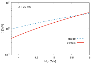
Figure 1: The total decay widths of the excited muon through the gauge and contact interaction for $\Lambda=20$ TeV.

Thus, We examined the production of the excited muon via contact interaction and decays to photon and muon via gauge interaction at TeV scale muon colliders in this paper. Our signal process is $\mu^{-}\mu^{+}\rightarrow\mu^{*}\mu^{+}\rightarrow\gamma\mu^{-}\mu^{+}$. We depicted the Feynman diagram of the signal process in Figure 5. Figure 5 represents the single production of the excited muon via contact interaction. In here, the excited muon decays to a photon and a muon via gauge interaction at TeV scale muon colliders. We calculated the total cross sections for the single production of the excited muon signal process $\mu^{-}\mu^{+}\rightarrow\mu^{*}\mu^{+}\rightarrow\gamma\mu^{-}\mu^{+}$ at muon collider with $\sqrt{s}=6$ TeV. Then we presented the total cross sections for single production of excited muons with $\Lambda=20$ and $30$ TeV in Figure 6. The compositeness scale value of the excited muon is taken as a higher value, as shown in Figure 6, that single production cross section values of the excited muon decrease.

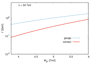
Figure 2: The total decay widths of the excited muon through the gauge and contact interaction with $\Lambda=30$ TeV.

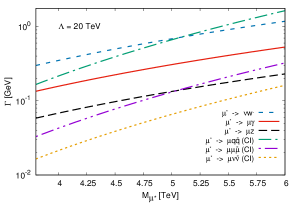
Figure 3: Partial decay widths of the excited muon via the contact and the gauge interactions with $\Lambda=20$ TeV.

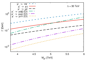
Figure 4: Partial decay width of the excited muon via the contact and the gauge interactions with $\Lambda=30$ TeV.

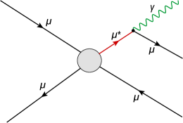
Figure 5: Feynman diagram for single production of an excited muon via the contact interaction at a muon collider. The excited muon decays via electromagnetic gauge interaction to a photon and a muon.

Figure 6: Total cross section for single production of the excited muon via contact interaction at muon collider with $\sqrt{s}=6$ TeV.

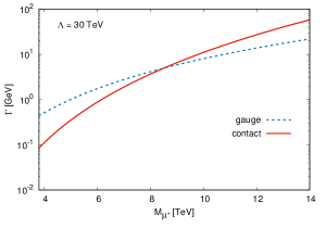
Figure 7: The total decay width of the excited muon for the contact and the gauge interactions with $\Lambda=30$ TeV.

3.2 14 TeV Muon Collider

As we mentioned in the previous subsection, we added the contact and gauge interaction Lagrangians of the excited leptons to the CalcHEP package program [96] using the LanHEP program [97, 98]. Then we used the CalcHEP package program and calculated the total decay width of the excited muon for the contact and the gauge interactions and plotted Figure 7 and Figure 8. One can see from Figure 7 that the gauge interaction mode dominates the contact interaction mode up to $8.4$ TeV for $\Lambda=20$ TeV. If we take the compositeness scale $\Lambda=50$ TeV, it can be seen from Figure 8 that the decay width of the excited muon via gauge interactions is more dominant than the decay width via contact interactions. We introduced the partial decay widths of the excited muon in Figure 9 and Figure 10. One can see from Figure 9 and Figure 10 , $\mu^{*}\rightarrow\nu W^{-}$, $\mu^{*}\rightarrow\mu^{-}q\bar{q}$, and $\mu^{*}\rightarrow\mu^{-}\gamma$ decay channels have larger decay width values than other decay channels. Here $q$ symbol represents $q=u,d,s,c,b,t$ the quarks. As mentioned in the previous sub-section, we chose as $\mu^{-}\mu^{+}\rightarrow\mu^{*}\mu^{+}\rightarrow\gamma\mu^{-}\mu^{+}$ the signal process for this reason. The total cross sections for single production via contact interaction and decays to photon and muon via gauge interaction of excited muon with $\Lambda=30$ and $\Lambda=50$ TeV at the center of mass-energy is $14$ TeV muon collider is shown in Figure 11. The compositeness scale value of the excited muon is taken as a higher value, as it is seen from Figure 11 that single production cross section values of the excited muon decrease.

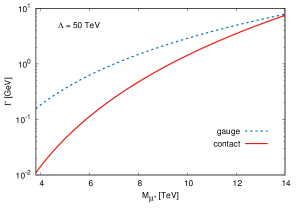
Figure 8: The total decay width of the excited muon for the contact and the gauge interactions with $\Lambda=50$ TeV.

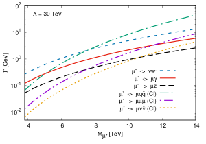
Figure 9: The partial decay width of excited muon via the contact and the gauge interactions with $\Lambda=30$ TeV.

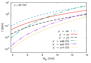
Figure 10: The partial decay width of excited muon via the contact and the gauge interactions with $\Lambda=50$ TeV.

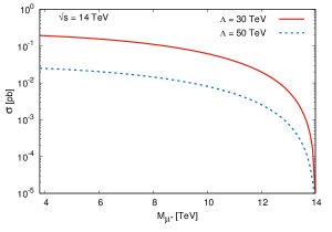
Figure 11: The total cross section for single production of the excited muon via contact interaction at muon collider with $\sqrt{s}=14$ TeV.

3.3 100 TeV Muon Collider

We computed the total decay width of the excited muon for the contact and the gauge interactions. We plotted Figure 12 and Figure 13. One can observe from Figure 12 that the gauge interaction mode dominates the contact interaction mode up to $43$ TeV for $\Lambda=150$ TeV. If we take the compositeness scale $\Lambda=300$ TeV, it can be noticed from Figure 13 that the decay width of the excited muon via the gauge interactions is more dominant than the decay width via the contact interactions. We presented the partial decay widths of the excited muon in Figure 14 and Figure 15. As seen from Figure 14, and Figure 15, $\mu^{*}\rightarrow\nu W^{-}$, $\mu^{*}\rightarrow\mu^{-}q\bar{q}$, and $\mu^{*}\rightarrow\mu^{-}\gamma$ decay channels have larger decay width values than other decay channels. Here $q$ symbol represents $q=u,d,s,c,b,t$ the quarks. For this reason, $\mu^{-}\mu^{+}\rightarrow\mu^{*}\mu^{+}\rightarrow\gamma\mu^{-}\mu^{+}$ process has been chosen as the signal process as in the previous subsection. Then we calculated the total cross-section for single production via the contact interaction and decays to photon and muon via the gauge interaction of the excited muon with $\Lambda=150$, $\Lambda=200$, and $\Lambda=300$ TeV at the center-of-mass energy is $\sqrt{s}=100$ TeV muon collider. After that, we plotted the total cross section for the excited muon’s single production as in Figure 16. The compositeness scale value of the excited muon is taken as a higher value, as seen from Figure 16, single production cross section values of the excited muon decrease.

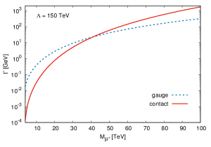
Figure 12: The total decay width of the excited muon for the contact and the gauge interactions with $\Lambda=150$ TeV.

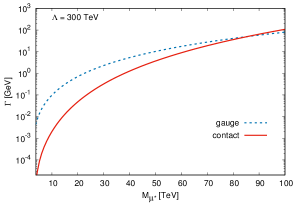
Figure 13: The total decay width of the excited muon for the contact and the gauge interactions with $\Lambda=300$ TeV.

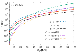
Figure 14: The partial decay width of excited muon via the contact and the gauge interactions with $\Lambda=150$ TeV.

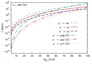
Figure 15: The partial decay width of excited muon via the contact and the gauge interactions with $\Lambda=300$ TeV.

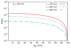
Figure 16: The total cross section for single production of the excited muon via the contact interaction at muon collider with $\sqrt{s}=100$ TeV.

4. SIGNAL AND BACKGOUND ANALYSIS

As addressed in the previous section, the $\mu^{*}\rightarrow\nu W^{-}$, $\mu^{*}\rightarrow\mu^{-}q\bar{q}$, and $\mu^{*}\rightarrow\mu^{-}\gamma$ partial decay channels of the excited muon are more dominant than the other decay channels. Consequently, we chose $\mu^{-}\mu^{+}\rightarrow\mu^{*}\mu^{+}\rightarrow\gamma\mu^{-}\mu^{+}$ as our signal process. According to this process, excited muon is produced at muon colliders through the contact interaction. Later, it decays into photon and muon via the gauge interactions. In this study, we could also choose the $\mu^{-}\mu^{+}\rightarrow\mu^{*}\mu^{+}\rightarrow q\bar{q}\mu^{-}\mu^{+}$ process for the signal process in which the excited muon is produced through the contact interactions and decay via the contact interactions. Here $q$ symbol represents $q=u,d,s,c,b,t$ the quarks. However, in this case, the number of final-state particles would be higher than the $\mu^{-}\mu^{+}\rightarrow\mu^{*}\mu^{+}\rightarrow\gamma\mu^{-}\mu^{+}$ process. For this reason, the background process’s cross section would be more since the number of particles in the final state would be higher. So it would be more challenging to separate the signal from the background. Hence, we chose $\mu^{-}\mu^{+}\rightarrow\mu^{*}\mu^{+}\rightarrow\gamma\mu^{-}\mu^{+}$ as the signal process. The background process that corresponds to this signal process is $\mu^{-}\mu^{+}\rightarrow\gamma\mu^{-}\mu^{+}$. As mentioned in the previous section, we added lagrangians to the CalcHEP simulation program via the LanHEP program. Those lagrangians representing excited leptons’ interactions with Standard Model fermions via the contact and the gauge interactions. We applied $p_{T}^{\gamma}>25$ GeV, $p_{T}^{\mu^{-}}>25$ GeV, $p_{T}^{\mu^{+}}>25$ GeV cut values for photon, muon and anti-muon of the final state particles in the signal and the background processes. Here $p_{T}$ represents the transverse momentum of the final state particles. Also, we applied the $\Delta R(\gamma\mu^{-})>0.7$, and $\Delta R(\gamma\mu^{+})>0.7$ cut value to separate the final state leptons from photons. Here $\Delta R$ is separation cuts, and $\Delta R=\sqrt{\Delta\eta^{2}+\Delta\phi^{2}}$.

4.1 Final State Particle Distributions and Significance Calculus at 6 TeV Muon Collider

In the present subsection, signal and background analysis are performed for the excited muon at 6 TeV center-of-mass energy collider predicted in the MAP and the LEMMA programs. Since the cross section of the background process is larger than the signal process’s cross section, it is not possible to identify the signal from the background with the acceptance cuts mentioned above. We needed the transverse momentum and the pseudorapidity distributions of the final state particles in the signal and background processes to determine the cuts to identify the signal over the background. It is observed that excited muon decay to photon and muon in the signal process. Since the muon and photon distributions are similar, we exhibited the photon’s transverse momentum and pseudorapidity distributions for the illustration. As shown in Figure 17, when the cut of $p_{T}^{\gamma}>400$ GeV is applied, this cut leaves the cross section value of the signal process almost unchanged. At the same time, it dramatically reduces the cross section value of the background process. Since the muon’s final state distribution is similar to the photon’s final state distribution, the same cut value $p_{T}^{\mu^{-}}>400$ GeV can be used for the muon. We plotted pseudorapidity distributions of final state photon and muon for the signal and the background process in Figures 18 and 19 . As shown in Figure 18, when the $-2.5<\eta^{\gamma}<2.5$ pseudorapidity cut interval is applied to the final state photon, the cross-section value of the signal remains almost unchanged. The background cross section value decreases. When Figure 19 is examined, during the $-4<\eta^{\mu^{-}}<1.5$ pseudorapidity cut interval is applied, the signal’s cross-section value remains almost unchanged, while the background cross-section value is significantly reduced. For all these reasons, we applied $p_{T}^{\gamma}>400$ GeV, $-2.5<\eta^{\gamma}<2.5$ cut values for the final state photon in the signal and the background processes. For the final state muon, we applied $p_{T}^{\mu^{-}}>400$ GeV, $-4<\eta^{\mu^{-}}<1.5$ cut values. We preferred to apply the cut values $p_{T}^{\mu^{+}}>400$ GeV, $-2.5<\eta^{\mu^{+}}<2.5$ for the final state anti-muon in the signal and the background processes. Besides, $|M_{\gamma\mu^{-}}-M_{\mu^{*}}|<500$ GeV mass window cut is another essential cut used to differentiate the signal from the background. We presented the cuts we determined as a result of all these inquiries in Equation 23.

$$p_{T}^{\gamma,\mu^{-},\mu^{+}}>400 \>GeV, -2.5<\eta^{\gamma,\mu^{+}}<2.5,$$

$$-4<\eta^{\mu^{-}}<1.5, \>\Delta R_{(\mu^{-}\gamma),(\mu^{+}\gamma)}>0.7$$ (23)

$$|M_{\gamma\mu^{-}}-M_{\mu^{*}}|<500 GeV$$

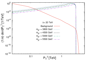
Figure 17: The transverse momentum distribution of final state photon for the signal and the background processes with $\Lambda=20$ TeV.

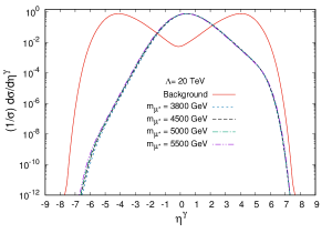
Figure 18: The pseudorapidity distribution of final state photon for the signal and the background processes with $\Lambda=20$ TeV.

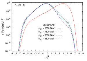
Figure 19: The pseudorapidity distribution of final state muon for the signal and the background processes with $\Lambda=20$ TeV.

We used Equation 24 for statistical significance calculation. Here $N_{s}$ represents the number of signal events and $N_{s}=\sigma_{s}\sqrt{L_{int}}$. $N_{B}$ in the Equation 24 represents the number of background events, and $N_{B}=\sigma_{B}L_{int}$. Also, the $\sigma_{s}$ represents the signal cross section, $\sigma_{B}$ represents the background cross section, and $L_{int}$ represents the integrated luminosity.

$$S=\frac{N_{s}}{\sqrt{N_{s}+N_{B}}}$$ (24)

We used cut sets in the Equation 23 and the integrated Luminosity values listed for the $6$ TeV center-of-mass energy of the muon collider in Table 1. Then, we have performed discovery ($5\sigma$), observation ($3\sigma$), and exclusion ($2\sigma$) analysis for the mass of the excited muon. Table 2 shows excited muon mass limits for the discovery ($5\sigma$), the observation ($3\sigma$), and the exclusion ($2\sigma$) at the muon collider with 6 TeV center-of-mass energy.

Table 2: The attainable mass limit for the excited muon at $6$ TeV muon collider.

$\sqrt{S}=6$ TeV
$L_{int}$	$510\>fb^{-1}$			$1200\>fb^{-1}$
Significance	$5\sigma$	$3\sigma$	$2\sigma$	$5\sigma$	$3\sigma$	$2\sigma$
$\Lambda=20$ TeV	$5.59$ TeV	$5.60$ TeV	$5.63$ TeV	$5.60$ TeV	$5.62$ TeV	$5.66$ TeV

So far, we have taken the compositeness scale as $\Lambda=20$ TeV in the calculations was performed. However, it is essential to determine the excited muon’s compositeness scale. Hence we scanned it by taking different values for the compositeness scale. Then we calculated the attainable compositeness scale limits for the excited muon at the muon collider with $\sqrt{S}=6$ TeV and $L_{int}=510\,fb^{-1}$. We plotted Figure 20 for the muon collider with $6$ TeV center-of-mass energy. Figure 20 represents the achievable compositeness scale limits versus the excited muon mass plot. As shown in the Figure 20 , the excited muon with mass $M_{\mu^{*}}=4$ TeV can be discovered up to $\Lambda=88.1$ TeV compositeness scale value for $L_{int}=510\,fb^{-1}$ at the muon collider with $6$ TeV center-of-mass energy. Similar calculations were made within $L_{int}=1200\,fb^{-1}$ total integrated luminosity value. Then we plotted Figure 21 . Figure 21 represents the attainable compositeness scale limits corresponding to the excited muon mass values plot. As illustrated in Figure 21, the excited muon with mass $M_{\mu^{*}}=4$ TeV can be discovered up to $99.2$ TeV compositeness scale value at the muon collider with $6$ TeV center of mass-energy and $L_{int}=1200\,fb^{-1}$. Detailed limit values regarding the achievable compositeness scale of the excited muon for the excited muon mass are listed in Table 3.

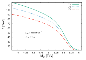
Figure 20: The compositeness scale versus the mass plots for the excited muon at $6$ TeV center-of-mass energy muon collider with $L_{int}=510\,fb^{-1}$.

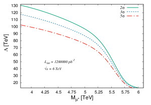
Figure 21: The compositenes scale versus the mass plots for the excited muon at $6$ TeV center-of-mass energy muon collider with $L_{int}=1200\,fb^{-1}$.

Table 3: The attainable compositeness scale limits for some excited muon mass values at muon collider with 6 TeV center-of-mass energy.

$\sqrt{S}=6$ TeV
$L_{int}$	$510\>fb^{-1}$			$1200\>fb^{-1}$
	Attainable Compositeness Scale ($\Lambda$)			Attainable Compositeness Scale ($\Lambda$)
Significance	$5\sigma$	$3\sigma$	$2\sigma$	$5\sigma$	$3\sigma$	$2\sigma$
$M_{\mu^{*}}=3.8$ TeV	$90.80$ TeV	$104.5$ TeV	$116.5$ TeV	$102.4$ TeV	$117.5$ TeV	$130.5$ TeV
$M_{\mu^{*}}=4.0$ TeV	$88.10$ TeV	$101.6$ TeV	$113.3$ TeV	$99.20$ TeV	$113.9$ TeV	$126.8$ TeV
$M_{\mu^{*}}=4.2$ TeV	$85.00$ TeV	$98.10$ TeV	$109.2$ TeV	$95.90$ TeV	$110.1$ TeV	$122.4$ TeV
$M_{\mu^{*}}=4.4$ TeV	$81.45$ TeV	$94.00$ TeV	$104.8$ TeV	$91.90$ TeV	$105.4$ TeV	$117.4$ TeV
$M_{\mu^{*}}=4.6$ TeV	$77.45$ TeV	$89.40$ TeV	$99.90$ TeV	$87.45$ TeV	$100.5$ TeV	$111.5$ TeV
$M_{\mu^{*}}=4.8$ TeV	$72.95$ TeV	$84.30$ TeV	$93.90$ TeV	$82.35$ TeV	$94.50$ TeV	$105.3$ TeV
$M_{\mu^{*}}=5.0$ TeV	$67.70$ TeV	$78.20$ TeV	$87.50$ TeV	$76.60$ TeV	$87.80$ TeV	$98.00$ TeV
$M_{\mu^{*}}=5.2$ TeV	$61.90$ TeV	$71.50$ TeV	$80.20$ TeV	$70.00$ TeV	$80.50$ TeV	$89.80$ TeV
$M_{\mu^{*}}=5.4$ TeV	$53.70$ TeV	$62.40$ TeV	$69.90$ TeV	$61.05$ TeV	$70.50$ TeV	$78.60$ TeV
$M_{\mu^{*}}=5.6$ TeV	$18.17$ TeV	$20.20$ TeV	$21.85$ TeV	$19.88$ TeV	$21.90$ TeV	$23.60$ TeV

As shown in Figures 20, 21, and Table 3, the muon collider with $6$ TeV center-of-mass energy will give an excellent potential search for a compositeness scale. Even this collider gives opportunity up to $100$ TeV compositeness scale value can be achieved.

4.2 Final State Particle Distributions and Significance Calculus at 14 TeV Muon Collider

We conducted a signal and background analysis for the excited muon at the muon collider with $\sqrt{s}=14$ TeV. It will be achieved using the LHC collider ring as a muon collider at the CERN. As illustrated at the beginning of chapter 4, we implemented lagrangians, which describe the gauge and the contact interactions of the excited leptons with the SM fermions, to the CalcHEP program through the LanHeP program. Our signal process is $\mu^{-}\mu^{+}\rightarrow\mu^{*}\mu^{+}\rightarrow\gamma\mu^{-}\mu^{+}$ and our background process is $\mu^{-}\mu^{+}\rightarrow\gamma\mu^{-}\mu^{+}$. For signal and background analysis, we applied generator level $p_{T}^{\gamma}>25$ GeV, $p_{T}^{\mu^{-}}>25$ GeV, $p_{T}^{\mu^{+}}>25$ GeV cut values for photon, muon and anti-muon of the final state particles in the signal and the background processes. Also, we applied the $\Delta R(\gamma\mu^{-})>0.7$, and $\Delta R(\gamma\mu^{+})>0.7$ cut value to separate the final state leptons from the photons. After that, we plotted the transverse momentum and the pseudorapidity distributions of the final state particles in the signal and the background processes to determine the cuts to identify the signal from the background. Since the final state of the muon and the photon distributions are similar, we exhibited the photon’s transverse momentum and pseudorapidity distributions for the illustration. Figure 22 shows the transverse momentum distributions of photons in the signal and the background processes. We took the compositeness scale as $\Lambda=30$ TeV, and the excited muon mass values are $M_{\mu^{*}}=3800,6000,8000,10000$, and $12000$ GeV in the final state particle distribution calculations. As shown in Figure 22, when we applied the cut $p_{T}^{\gamma}>500$ GeV for the final state photon, this cut leaves the cross-section value of the signal process almost unchanged. At the same time, it dramatically reduces the cross-section value of the background process. Since the muon’s final state distribution is similar to the photon’s final state distribution, the same cut value $p_{T}^{\mu^{-}}>500$ GeV can be used for the muon. We plotted pseudorapidity distributions of final state photon and muon for the signal and the background process in Figures 23 and 24. As illustrated in Figure 23, when the $-3<\eta^{\gamma}<3$ pseudorapidity cut interval is applied to the final state photon, the cross-section value of the signal remains almost unchanged. The background cross-section value decreases. When Figure 24 is examined, during the $-4<\eta^{\mu^{-}}<2.5$ pseudorapidity cut interval is applied, the signal’s cross-section value remains almost unchanged, while the background cross-section value is significantly reduced. For all these reasons, we applied $p_{T}^{\gamma}>500GeV$, $-3<\eta^{\gamma}<3$ cut values for the final state photon in the signal and the background processes. For the final state muon, we applied $p_{T}^{\mu^{-}}>500GeV$, $-4<\eta^{\mu^{-}}<2.5$ cut values. Also, we preferred to apply the cut values $p_{T}^{\mu^{+}}>500GeV$, $-2.5<\eta^{\mu^{+}}<2.5$ for the final state anti-muon in the signal and the background processes. Besides, $|M_{\gamma\mu^{-}}-M_{\mu^{*}}|<500$ GeV mass window cut is another essential cut used to identify the signal from the background. We summarized all of these cuts we determined to use in signal and background analysis at the muon collider with 14 TeV center-of-mass energy in the Equation 25.

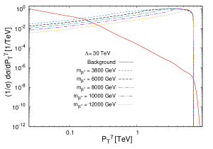
Figure 22: The transverse momentum distribution of final state photon for the signal and the background processes with $\Lambda=30$ TeV.

Figure 23: The pseudorapidity distribution of final state photon for the signal and the background processes with $\Lambda=30$ TeV

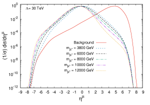
Figure 24: The pseudorapidity distribution of final state muon for the signal and the background processes with $\Lambda=30$ TeV

$$p_{T}^{\gamma,\mu^{-},\mu^{+}}>500 GeV, -3<\eta^{\gamma}<3,$$

$$-4<\eta^{\mu^{-}}<2.5, -2.5<\eta^{\mu^{+}}<2.5$$ , (25)

$$\Delta R_{(\mu^{-}\gamma),(\mu^{+}\gamma)}>0.7, |M_{\gamma\mu^{-}}-M_{\mu^{*}}|<500 GeV$$

Using the statistical significance formula in the Equation 24 and all cuts summarized in the Equation 25, we calculated the achievable mass limits for excited muons at the muon collider with 14 TeV center-of-mass energy. Then, we listed discovery ($5\sigma$), observation ($3\sigma$), and exclusion ($2\sigma$) limits for the mass of the excited muon in Table 4. As can be seen from Table 4, for $L_{int}=12\,fb^{-1}$, the excited muon can be discovered up to $13.26$ TeV at the muon collider with $14$ TeV center-of-mass energy. High Luminosity Large Hadron Collider (HL-LHC) can not reach this limit value even in its entire working lifetime. From this, it can be said that the muon colliders will be a very effective collider.

Table 4: The attainable mass limit for the excited muon at $14$ TeV muon collider.

$\sqrt{S}=14$ TeV
$L_{int}$	$2.4\>fb^{-1}$			$12\>fb^{-1}$
Significance	$5\sigma$	$3\sigma$	$2\sigma$	$5\sigma$	$3\sigma$	$2\sigma$
$\Lambda=30$ TeV	$12.52$ TeV	$13.08$ TeV	$13.31$ TeV	$13.26$ TeV	$13.43$ TeV	$13.48$ TeV

Up to now, we performed all calculations for $\Lambda=30$ TeV in this sub-section. However, the compositeness scale of the excited muon may have values other than $30$ TeV. Therefore, we did a compositeness scale scan for each different excited muon mass. Figure 25 represents the compositeness scale plot for $L_{int}=2.4\,fb^{-1}$ depending on the mass of the excited muon. As depicted in Figure 25, the excited muon with a mass value of $3.8$ TeV will be discovered at the muon collider up to $\Lambda=60.45$ TeV compositeness scale value. Figure 26 represents the compositeness scale plot for $L_{int}=12\,fb^{-1}$ depending on the mass of the excited muon. As seen in Figure 26, the excited muon with a mass value of $3.8$ TeV will be discovered up to a compositeness scale value of $\Lambda=89.14$ TeV. The detailed compositeness scale limits obtained depending on the mass of the excited muon are listed in Table 5. According to Table 5, the excited muon with $10$ TeV mass will be discovered up to a compositeness scale of approximately $69$ TeV at the muon collider with $14$ TeV center-of-mass energy. The results show that the $14$ TeV center-of-mass energy muon collider will be a good alternative to Hadron-Hadron colliders to investigate the excited muon, although it has low integrated luminosity values.

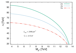
Figure 25: The compositeness scale versus the mass plots for the excited muon at $14$ TeV center-of-mass energy muon collider with $L_{int}=2.4\,fb^{-1}$.

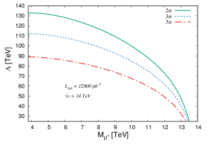
Figure 26: The compositeness scale versus the mass plots for the excited muon at $14$ TeV center-of-mass energy muon collider with $L_{int}=12\,fb^{-1}$.

Table 5: The attainable compositeness scale limits for some excited muon mass values at the muon collider with $14$ TeV center-of-mass energy.

$\sqrt{S}=14$ TeV
$L_{int}$	$2.4\>fb^{-1}$			$12\>fb^{-1}$
	Attainable Compositeness Scale ($\Lambda$)			Attainable Compositeness Scale ($\Lambda$)
Significance	$5\sigma$	$3\sigma$	$2\sigma$	$5\sigma$	$3\sigma$	$2\sigma$
$M_{\mu^{*}}=3.8$ TeV	$60.45$ TeV	$77.54$ TeV	$93.86$ TeV	$89.14$ TeV	$112.2$ TeV	$132.7$ TeV
$M_{\mu^{*}}=5.0$ TeV	$59.65$ TeV	$76.58$ TeV	$92.88$ TeV	$88.15$ TeV	$111.3$ TeV	$132.1$ TeV
$M_{\mu^{*}}=6.0$ TeV	$58.25$ TeV	$74.78$ TeV	$90.68$ TeV	$86.07$ TeV	$108.7$ TeV	$128.9$ TeV
$M_{\mu^{*}}=7.0$ TeV	$56.32$ TeV	$72.27$ TeV	$87.60$ TeV	$83.15$ TeV	$104.9$ TeV	$124.3$ TeV
$M_{\mu^{*}}=8.0$ TeV	$53.82$ TeV	$69.03$ TeV	$83.58$ TeV	$79.36$ TeV	$99.93$ TeV	$118.2$ TeV
$M_{\mu^{*}}=9.0$ TeV	$50.65$ TeV	$64.92$ TeV	$78.53$ TeV	$74.59$ TeV	$93.75$ TeV	$110.7$ TeV
$M_{\mu^{*}}=10$ TeV	$46.66$ TeV	$59.77$ TeV	$72.20$ TeV	$68.62$ TeV	$86.05$ TeV	$101.3$ TeV
$M_{\mu^{*}}=11$ TeV	$41.53$ TeV	$53.17$ TeV	$64.18$ TeV	$61.00$ TeV	$76.38$ TeV	$89.82$ TeV
$M_{\mu^{*}}=12$ TeV	$34.68$ TeV	$44.44$ TeV	$53.70$ TeV	$51.03$ TeV	$63.99$ TeV	$73.36$ TeV
$M_{\mu^{*}}=13$ TeV	$24.40$ TeV	$31.39$ TeV	$38.12$ TeV	$36.16$ TeV	$45.77$ TeV	$54.40$ TeV

4.3 Final State Particle Distributions and Significance Calculus at $100$ TeV Muon Collider

In this subsection, we performed a signal background analysis for the excited muon at the 100 TeV center-of-mass energy muon collider, which will be obtained using the FCC collider ring as a muon collider at the CERN. As we mentioned at the beginning of chapter 4, our signal process is $\mu^{-}\mu^{+}\rightarrow\mu^{*}\mu^{+}\rightarrow\gamma\mu^{-}\mu^{+}$, and the background process is $\mu^{-}\mu^{+}\rightarrow\gamma\mu^{-}\mu^{+}$. Firstly, we put acceptance cuts $p_{T}^{\gamma}>25$ GeV, $p_{T}^{\mu^{-}}>25$ GeV, $p_{T}^{\mu^{+}}>25$ GeV on muon, photon and, anti-muon, respectively. In addition to these acceptance cuts, we used $-2.5<\eta^{\mu^{+}}<2.5$ pseudorapidity interval for anti-muon and $\Delta R(\gamma\mu^{-})>0.7$, and $\Delta R(\gamma\mu^{+})>0.7$ acceptance cuts for the separation photon from muon and anti-muon. Since these cuts are not sufficient to identify the signal from the background, we plotted the transverse momentum and the pseudorapidity distributions of the photon, muon, and anti-muon, which are the final state particles of the signal and the background processes. We performed calculations for $\Lambda=150$ TeV and $M_{\mu^{*}}=5000$, $10000$, $20000$, $30000$, $40000$, $50000$, $60000$, and $70000$ GeV in this sub-section. Figure 27 represents the transverse momentum distributions of the final state photons in the signal and the background processes. When we applied the cut $p_{T}^{\gamma}>500$ GeV for the final state photon, this cut leaves the cross-section value of the signal process almost unchanged, while it dramatically reduces the cross-section value of the background process. Since the muon’s final state distribution is similar to the photon’s final state distribution, the same cut value $p_{T}^{\mu^{-}}>500$ GeV can be used for the muon. We plotted pseudorapidity distributions of final state photon and muon for the signal and the background process in Figures 28 and 29. As illustrated in Figure 28, while the $-3<\eta^{\gamma}<3.5$ pseudorapidity cut interval is applied to the final state photon, the cross-section value of the signal remains almost unchanged the background cross-section value decreases. When Figure 29 is examined, during the $-4<\eta^{\mu^{-}}<3.5$ pseudorapidity cut interval is applied, the signal’s cross-section value remains almost unchanged, while the background cross-section value is significantly reduced. Because of all these reasons, we applied $p_{T}^{\gamma}>500$ GeV, $-3<\eta^{\gamma}<3.5$ cut values for the final state photon in the signal and the background processes. For the final state muon, we applied $p_{T}^{\mu^{-}}>500$ GeV, $-4<\eta^{\mu^{-}}<3.5$ cut values. Also, we preferred to apply the cut values $p_{T}^{\mu^{+}}>500$ GeV, $-2.5<\eta^{\mu^{+}}<2.5$ for the final state anti-muon in the signal and the background processes. Moreover, $|M_{\gamma\mu^{-}}-M_{\mu^{*}}|<500$ GeV mass window cut is another essential cut used to identify the signal from the background. We overview all of these cuts we determined to use in signal and the background analysis at the muon collider with 100 TeV center-of-mass energy in Equation 12.

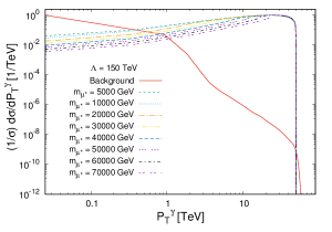
Figure 27: The transverse momentum distribution of final state photon for the signal and the background processes with $\Lambda=150$ TeV.

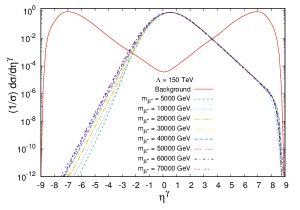
Figure 28: The pseudorapidity distribution of final state photon for the signal and the background processes with $\Lambda=150$ TeV

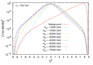
Figure 29: The pseudorapidity distribution of final state muon for the signal and the background processes with $\Lambda=150$ TeV.

$$p_{T}^{\gamma,\mu^{-},\mu^{+}}>500 GeV, -3<\eta^{\gamma}<3.5,$$

$$-4<\eta^{\mu^{-}}<3.5, -2.5<\eta^{\mu^{+}}<2.5,$$ (26)

$$\Delta R_{(\mu^{-}\gamma),(\mu^{+}\gamma)}>0.7, |M_{\gamma\mu^{-}}-M_{\mu^{*}}|<500GeV$$

We used the statistical significance formula of Equation 10, cut set in Equation 12, and an integrated luminosity value for a muon collider with $100$ TeV center-of-mass energy in Table 1. Then, we calculated discovery ($5\sigma$), observation ($3\sigma$), and exclusion ($2\sigma$) limits for the excited muon with $\Lambda=150$ TeV. As a result of the calculations, the excited muon will be discovered up to $94.20$ TeV, observed up to $96.53$ TeV, and excluded up to $97.66$ TeV at the muon collider with $100$ TeV center-of-mass energy for $L_{int}=100\,fb^{-1}$. The fact that the excited muon will be discovered at the muon collider up to $94.20$ TeV is a very high mass value for the excited muon. It indicates that the muon colliders will be a very effective collider for an excited muon.

We did calculations for the excited muon in this sub-section; we took the value of the compositeness scale has been taken as $\Lambda=150$ TeV up to now. However, for each mass of the excited muon, the compositeness scale can take different values. Therefore, we calculated the upper limits for the compositeness scale for some excited muon masses at muon collider with the $100$ TeV center-of-mass energy. The excited muon with a mass of $20$ TeV will be discovered up to $425.2$ TeV compositeness scale value for $L_{int}=100\,fb^{-1}$. The excited muon with a mass of $90$ TeV will be discovered up to $198.6$ TeV compositeness scale value. As can be seen from these values, the muon collider with $100$ TeV center-of-mass energy and $L_{int}=100\,fb^{-1}$ will be able to discover the excited muon even if it has very high compositeness scale values. We listed the detailed results in table 6.

Table 6: The attainable compositeness scale limits for some excited muon mass values at the muon collider with $100$ TeV center-of-mass energy.

$\sqrt{S}=100$ TeV with $L_{int}=100\,fb^{-1}$
	Attainable Compositeness Scale ($\Lambda$)
Significance	$5\sigma$	$3\sigma$	$2\sigma$
$M_{\mu^{*}}=20$ TeV	$425.2$ TeV	$546.9$ TeV	$665.5$ TeV
$M_{\mu^{*}}=50$ TeV	$384.8$ TeV	$495.7$ TeV	$604.2$ TeV
$M_{\mu^{*}}=70$ TeV	$323.6$ TeV	$417.4$ TeV	$509.3$ TeV
$M_{\mu^{*}}=90$ TeV	$198.6$ TeV	$258.0$ TeV	$315.6$ TeV

5. CONCLUSION

We investigated the excited muon production via the contact interaction and decays to the SM fermions through photon radiation at the muon colliders. The calculations were performed at the muon colliders with $6$ TeV, $14$ TeV, and $100$ TeV center-of-mass energy options. The excited muon will be discovered up to $5.60$ TeV mass value for $\Lambda=20$ TeV at the muon collider with $6$ TeV center-of-mass energy, and $L_{int}=1200$$\,fb^{-1}$ integrated luminosity. It is seen that this value is close to the center-of-mass energy value of the collider. At the muon collider with $14$ TeV center-of-mass energy and $12\,fb^{-1}$ integrated luminosity, the excited muon will be discovered up to $13.26$ TeV for $\Lambda=30$ TeV. This limit value is also close to the center-of-mass energy of the collider. Since the High Luminosity Large Hadron Collider is a hadron-hadron collider, It will not reach this mass limit for the excited muon even during its entire run time. Moreover, the excited muon will be discovered up to $94.20$ TeV mass value for $\Lambda=150$ TeV at the muon collider with $100$ TeV center-of-mass energy and $L_{int}=100\,fb^{-1}$ integrated luminosity. As with other center-of-mass energy options, this limit value is close to the collider’s center-of-mass energy value. Because the FCC proton-proton collider is a hadron-hadron collider, it will not reach this mass limit even during its entire run time. All these results show that the muon colliders will be a perfect collider option for examining the excited muon. These limits on the mass of the excited muon at all center-of-mass energy options for the muon colliders are shown in Figure 30.

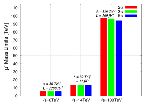
Figure 30: The excited muon mass limits at various center-of-mass energy muon colliders.

An excited muon with a $4$ TeV mass will be discovered at the muon collider with a $6$ TeV center-of-mass energy and $L_{int}=1200\,fb^{-1}$ up to $99.20$ TeV compositeness scale. At the muon collider with $14$ TeV center-of-mass energy and $L_{int}=12\,fb^{-1}$, the excited muon with a $5$ TeV mass will be discovered up to $88.15$ TeV compositeness scale value. Also, the excited muon with $20$ TeV mass will be discovered up to 425.2 TeV compositeness scale at the muon collider with $100$ TeV center-of-mass energy and $L_{int}=100\,fb^{-1}$. As can be seen from all these data, the excited muon can be examined up to very high compositeness scale values at the muon collider. In other words, the muon colliders will be able to determine the compositeness scale value of the excited muon.

All these calculations about the excited muon show that the muon colliders will be a unique collider search for the excited muon.Since the mass of the muon is greater than the electron, it loses less energy in the acceleration process. Therefore, it will be easier to increase the momentum of the muons to higher energies at accelerators. For all these reasons, many Standard Model and Beyond Standard Model processes will be investigated better than other types of colliders through the muon anti-muon colliders.