Stitch Fix for Mapper and Topological Gains

Abstract

The mapper construction is a powerful tool from topological data analysis that is designed for the analysis and visualization of multivariate data. In this paper, we investigate a method for stitching a pair of univariate mappers together into a bivariate mapper, and study topological notions of information gains, referred to as topological gains, during such a process. We further provide implementations that visualize such topological gains for mapper graphs.

1 Introduction

The mapper construction is one of the main tools in topological data analysis and visualization used for the study of multivariate data SinghMemoliCarlsson2007 . It takes as input a multivariate function defined on the data and produces a topological summary of the data using a cover of the range space of the function. For a given cover, such a summary converts the mapping into a simplicial complex suitable for data exploration.

In this paper, we take a constructive viewpoint of a multivariate function $f:{{\mathbb{X}}}\to{{\mathbb{R}}}^{d}$ defined on a topological space ${{\mathbb{X}}}$ and consider it as a vector of continuous, real-valued functions defined on a shared domain, $f=(f_{1},f_{2},\cdots,f_{d}),f_{i}:{{\mathbb{X}}}\to{{\mathbb{R}}}$, where each $f_{i}$ (referred to as a filter function) gives rise to a univariate mapper (or mapper construction). We investigate a method for stitching a pair of univariate mappers together and study topological notions of information gains, referred to as topological gains, from such a process. Our notion of topological gain is loosely inspired by the concept of information gain used in the construction of decision trees, which is computed by comparing the entropy of the dataset before and after a transformation. Topology gain, in our context, measures the change in topological information by comparing the homology or entropy of the mapper before and after the stitching process. In particular, we aim to assign a measure that captures information about how each filter function contributes to the topological content of the stitched result, and how the two filter functions are topologically correlated.

We are also inspired by the ideas of stepwise regression for model selection and scatterplot matrices for visualization. For a set of variables $x_{1},x_{2},\ldots,x_{d}$, the stepwise regression Efroymson1960 ; Hocking1976 iteratively incorporates variables into a regression model based on some criterion. A measure of topological gain can be used as a criterion for choosing filter functions and constructing a single “best” multivariate mapper. The scatterplot matrix ElmqvistDragicevicFekete2008 shows all pairwise scatterplots for the set of variables on a single $d\times d$ matrix, where each scatterplot illustrates the degree of correlation between two variables. We are interested in a topological analogue of the scatterplot matrix for a set of filter functions $f_{1},f_{2},\ldots,f_{d}$, referred to as mapper matrix, and in studying the degree of topological correlation between filter functions.

Contributions. Our contributions are as follows:

• We define a composition (or stitching) operation for mappers (Definition 1) and show its equivalence to the standard construction (Theorem 3.1). We then provide an algorithm for carrying out this composition (Algorithm 1). Although the composition produces identical results as the standard construction, we focus on interrogating the composition process itself to study and quantify structural differences between a bivariate mapper and its corresponding univariate mappers.

• We consider three measures that quantify topological gains during the stitching process (Sect. 6). To the best of our knowledge, this is the first time information-theoretic measures are used in the study of mapper constructions.

• We end by describing our efforts in studying topological gains between filter functions via interactive visualization of a mapper graph matrix, using synthetic and real-world datasets.

• Our visualization tool is open source via GitHub at https://github.com/tdavislab/mapper-stitching.

2 Related Work

The mapper construction can be considered as a discrete approximation MunchWang2016 of the Reeb space EdelsbrunnerHarerPatel2008 , which is a topological descriptor of a multivariate function. The Reeb graph is a special type of a Reeb space for a univariate function, which has been actively studied in recent years BiasottiGiorgiSpagnuolo2008 . Similarly, the mapper graph is a special type of mapper for a univariate function, approximating the Reeb graph under certain conditions BrownBobrowskiMunch2020 . The mapper construction has emerged as a practical and effective tool to solve a number of problems in data science Alagappan2012 ; LumSinghLehman2013 ; NicolauLevineCarlsson2011 ; RoblesHajijRosen2018 ; SaggarSpornsGonzalez-Castillo2018 . The mapper construction has a number of variants, including the $\alpha$-Reeb graph ChazalSun2014 , extended Reeb graph BarralBiasotti2014 , multi-resolutional Reeb graph HilagaShinagawaKohmura2001 , multiscale mapper DeyMemoliWang2016 , multinerve mapper CarriereOudot2018 , joint contour net CarrDuke2013 ; CarrDuke2014 , and enhanced mapper graphs BrownBobrowskiMunch2020 ; see YanMasoodSridharamurthy2021 for a survey.

Although the mapper construction has been widely appreciated by the practitioners, many open questions remain regarding its theoretical properties, such as its information content CarriereOudot2018 ; DeyMemoliWang2017 ; GasparovicGommelPurvine2018 , stability BrownBobrowskiMunch2020 ; CarriereOudot2018 , and convergence Babu2013 ; DeyMemoliWang2017 ; MunchWang2016 ; SinghMemoliCarlsson2007 ; see BrownBobrowskiMunch2020 for a discussion. The mapper construction can be considered as a “lossy compression” of the information from the original data. To quantify its information content, Dey et al. DeyMemoliWang2017 showed that the 1-dimensional homology of the mapper is no richer than the domain itself. Carriére and Oudot CarriereOudot2018 quantified the information encoded in the mapper using the extended persistence diagram of its corresponding Reeb graph. Different from previous approaches, our work quantifies the topological gain (in an information-theoretic sense) of a bivariate mapper when it is constructed by stitching a pair of univariate mappers.

There are several open-source implementations of the mapper algorithm, including Python Mapper MullnerBabu2013 , KeplerMapper VeenSaulEargle2019 ; VeenSaulEargle2019b , giotto-tda library TauzinLupoTunstall2020 , Gudhi GUDHI2020 , Mapper Interactive ZhouChalapathiRathore2021 , and its domain-specific adaptations KamruzzamanKalyanaramanKrishnamoorthy2019 ; ZhouKamruzzamanSchnable2021 . In particular, Mapper interactive provides a simple but effective strategy for speeding up mapper graph computations by precomputing the distance matrix of points within each interval using a highly optimized function within scikit-learn ZhouChalapathiRathore2021 ; it also comes with a GPU implementation.

Hajij et al. HajijAssiriRosen2020 studied the computation of mapper in parallel. The main idea is to decompose the computation onto a set of processors by decomposing the space of interest into multiple smaller, partially overlapping subspaces. Each subspace is processed independently by a processing unit, resulting in a mapper construction on the subspace. The final mapper graph on the entire space is obtained by merging together the individual pieces gathered from subspaces.

In comparison with the work of Hajij et al. HajijAssiriRosen2020 , we focus on a completely different problem. Their approach HajijAssiriRosen2020 produces a final mapper graph by stitching together mapper graphs constructed from spatially distributed individual subspaces; while our Algorithm 1, in the univariate setting, produces a final mapper graph by stitching together mapper graphs constructed from individual filter functions. Specifically, each filter function gives rise to a univariate mapper. We stitch two univariate mappers into a bivariate mapper and study the topological gains from the stitching process using information theory. In the univariate setting, although both approaches produce the same final mapper graph, our work is not about the efficient computation of the mapper construction, but rather, we care about the stitching process itself and how much information is gained during the stitching process, moving from a univariate mapper to a multivariate mapper.

3 Main Theoretical Result

We assume the readers are familiar with concepts in algebraic and computational topology such as homology (see the book by Edelsbrunner and Harer EdelsbrunnerHarer2010 for an introduction). Given a space ${{\mathbb{X}}}$, a function $f:{{\mathbb{X}}}\to{{\mathbb{R}}}^{d}$, and a cover $\mathcal{U}=\{U_{i}\}$ of $f({{\mathbb{X}}})$, we define the pullback cover $f^{*}(\mathcal{U})$ of ${{\mathbb{X}}}$ as the cover obtained by decomposing each $f^{-1}(U_{i})$ into its path-connected components $\cup_{j=1}^{k_{i}}u_{ij}$. The mapper SinghMemoliCarlsson2007 is then a simplicial complex defined as the nerve of this pullback cover $M(f,\mathcal{U}):=\mathrm{Nrv}(f^{*}(\mathcal{U}))$.

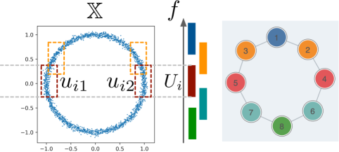
Figure 1: The mapper of a height function $f$ defined on a 2-dimensional point cloud sample ${{\mathbb{X}}}$ of a circle. Mapper parameters: $n=5$, $p=33\%$.

For simplicity, we describe the mapper construction by assuming ${{\mathbb{X}}}$ to be a point cloud equipped with a univariate function $f:{{\mathbb{X}}}\to{{\mathbb{R}}}$. Several parameters are relevant to the construction of its mapper. First is the number of intervals (of uniform lengths) in the cover $\mathcal{U}$ of $f({{\mathbb{X}}})$, denoted as $n$ and referred to as the resolution, giving the cover $\mathcal{U}=\{U_{1},\dots,U_{n}\}$. Second is the amount of overlap $p$ between the intervals in $\mathcal{U}$ (e.g., $20\%$ overlap). Finally, there are parameters associated with a clustering algorithm (e.g., DBSCAN EsterKriegelSander1996 ) that clusters points in $f^{-1}(U_{i})$ into connected components. These clusters of points form a pullback cover of ${{\mathbb{X}}}$, and the mapper is the nerve of such a cover. An example of a univariate mapper is shown in Fig. 1 for a height function $f:{{\mathbb{X}}}\to{{\mathbb{R}}}$ defined on a 2-dimensional point cloud sample of a circle, for $n=5$ and $p=33\%$. Note that the inverse $f^{-1}(U_{i})$ of the red interval $U_{i}$ is decomposed into two clusters $u_{i1}$ and $u_{i2}$, forming part of the pullback cover of ${{\mathbb{X}}}$.

On the other hand, if $f$ becomes a bivariate function, $f=(f_{1},f_{2})$ for $f_{i}:{{\mathbb{X}}}\to{{\mathbb{R}}}$ ($i=1,2$), then the cover of $f({{\mathbb{X}}})$ consists of rectangles and the resulting mapper is referred to as a bivariate mapper.

Definition 1 (Composition)

Given $f,g:{{\mathbb{X}}}\to{{\mathbb{R}}}$ and covers $\mathcal{U}=\{U_{i}\}$ and $\mathcal{V}=\{V_{j}\}$ of their respective images $f({{\mathbb{X}}})$ and $g({{\mathbb{X}}})$, we construct a composed cover $\mathcal{W}$ of ${{\mathbb{X}}}$ from $f^{*}(\mathcal{U})$ and $g^{*}(\mathcal{V})$ by taking the connected components of the set $\{U^{\prime}\cap V^{\prime}\mid\forall U^{\prime}\in f^{*}(\mathcal{U}),\forall V^{\prime}\in g^{*}(\mathcal{V}),U^{\prime}\cap V^{\prime}\neq\emptyset\}$, where $U^{\prime}\in f^{*}(\mathcal{U})$ and $V^{\prime}\in g^{*}(\mathcal{V})$ are path-connected cover elements of ${{\mathbb{X}}}$:

$$\mathcal{W}= \{W_{k}\mid\cup_{k}W_{k}=U^{\prime}\cap V^{\prime},\forall U^{\prime}\in f^{*}(\mathcal{U}),\forall V^{\prime}\in g^{*}(\mathcal{V}),U^{\prime}\cap V^{\prime}\neq\emptyset,$$

$$~{}~{}W_{k}\text{ is path-connected}\}.$$

We define the composed mapper as the nerve of this cover $\mathcal{W}$,

$$S(M(f,\mathcal{U}),M(g,\mathcal{V})):=\mathrm{Nrv}(\mathcal{W}).$$

Under certain assumptions, this composition $S$ is equivalent to the traditional method of constructing mappers from a pair of filter functions, as described by Theorem 3.1.

Theorem 3.1

If $f$ and $g$ are continuous real-valued functions, $U_{i}$, $V_{j}$, and $U_{i}\times V_{j}$ are simply connected for all $i,j$, then $S(M(f,\mathcal{U}),M(g,\mathcal{V}))=M((f,g),\mathcal{U}\times\mathcal{V})$, the bivariate mapper constructed in the traditional manner.

Proof sketch. The proof follows directly from properties of continuous functions and connected sets. We provide a sketch here. Starting with the two covers associated with the two univariate mappers, $\mathcal{U}$ for $f$ and $\mathcal{V}$ for $g$, we can show that the defined set $\mathcal{W}$ and the cover obtained from the traditional mapper construction are equivalent. Taking the nerve of each, we conclude that the resulting mappers are equivalent as well. See Sect. 5 for details.

Furthermore, we give an algorithm (Algorithm 1) that illustrates how the composition can be considerably simplified by directly incorporating simplex information from each of the two input mappers. The algorithm that combines (or stitches) two mappers together works by tracking vertices (i.e., representatives of the path-connected pull back cover elements as a result of the $\mathrm{Nrv}$ operation) of the first mapper in a breadth first search fashion and combining them with vertices of the second mapper. The simplices in both mappers provide hints about which possible simplices could be in the composition. Using this information to avoid many explicit intersection checks, we can considerably simplify and speed up the composition process. Although some simplices from each univariate mapper can be added directly to the composition (the STITCH step), others require explicitly checking the nerve condition in the mapper construction (the FIX step).

We recall the relevant notation used in the following sections. Given $f,g:{{\mathbb{X}}}\to{{\mathbb{R}}}$, let $\mathcal{U}=\{U_{i}\}$ and $\mathcal{V}=\{V_{j}\}$ denote the cover of their images $f({{\mathbb{X}}})$ and $g({{\mathbb{X}}})$, respectively. Let $\{U^{\prime}\}$ and $\{V^{\prime}\}$ denote the sets of path-connected cover elements of ${{\mathbb{X}}}$ in the pullback covers, $f^{*}(\mathcal{U})$ and $f^{*}(\mathcal{V})$, respectively. Let $\{u\}$ and $\{v\}$ represent the set of vertices in the mappers $M(f,\mathcal{U})$ and $M(g,\mathcal{V})$, respectively. Let $\mathcal{W}=\{W\}$ denote the composed cover of ${{\mathbb{X}}}$, and $\{w\}$ the set of vertices for the composed cover, that is, $w=\mathrm{Nrv}(W)$.

4 Algorithm

The stitching (composition) algorithm, as shown in Algorithm 1, has two main phases, STITCH for each cover element and FIX across cover elements. The STITCH phase takes all vertices from the first mapper in each cover element and stitches them together with all vertices in the second mapper. All simplices within the cover element of the second mapper will be inherited in the composition. The second phase FIX addresses simplices that cross between cover elements and uses an auxiliary procedure COMPLETE to construct simplices that cannot be derived directly from simplices in either of the two input mappers.

Suppose we have two filter functions, $f,g:{{\mathbb{X}}}\to{{\mathbb{R}}}$ together with covers of their images, $\mathcal{U}=\{U_{i}\}$ and $\mathcal{V}=\{V_{j}\}$. We define a function, $\mu(\cdot)$ that takes a vertex $v$ in $M(f,\mathcal{U}):=\mathrm{Nrv}(f^{*}(\mathcal{U}))$ and returns a path-connected cover element of ${{\mathbb{X}}}$ to which the vertex belongs. For a cover element $U_{i}\in\mathcal{U}$ (referred to as an interval set of $f({{\mathbb{X}}})$), we consider a vertex $v\in M(f,\mathcal{U})$ to be in the interval set $U_{i}$ if $f(\mu(v))\subseteq U_{i}$. We say a simplex $\sigma$ satisfies the nerve condition if $\cap_{i}\mu(v_{i})\neq\emptyset$ for all $v_{i}\subset\sigma$.

For each cover element $U_{i}\in\mathcal{U}$, the algorithm iterates over each path-connected component of $f^{*}(U_{i})\cap g^{*}(\mathcal{V})$. Hence there exists a unique cover element $W_{jh}$ of ${{\mathbb{X}}}$ in $\{W\}$ in Line 5 of STITCH for $v_{j}$ corresponding to the $h$-th component (for some $h$) in $\mu(v_{j})\cap f^{*}(U_{i})$. Also, vertex $u$ in Line 3 of FIX is unique.

In Algorithm 1, the set $\{u\}$ and $\{v\}$ contain vertices whereas the set $\{W\}$ contains path-connected cover elements of ${{\mathbb{X}}}$ (we use vertex $w$ for $\mathrm{Nrv}(W)$). We make use of the notion of $p$-completion in COMPLETE. For a $p$-dimensional simplicial complex $\Sigma$, its $p$-dimensional completion GundertSzedlak2015 is defined to be:

$$\Sigma\cup\left\{\tau\in\binom{\Sigma^{(0)}}{p\text{+}1}\Big{\lvert}\,(\tau\setminus v)\in\Sigma,\forall v\in\tau\right\},$$

where $\Sigma^{(0)}$ is the vertex set of $\Sigma$. In our use, we reduce the set to include only simplices that satisfy the nerve condition. We illustrate the steps of Algorithm 1 on a simple space ${{\mathbb{X}}}$ in Fig. 2.

Algorithm 1 Mapper Composition

1:$M(f,\mathcal{U}),~{}M(g,\mathcal{V})$

2:$S(M(f,\mathcal{U}),M(g,\mathcal{V}))$

3:$M\leftarrow\{\}$ $\triangleright$ An empty simplicial complex

4:$\mathcal{W}\leftarrow\{\}$ $\triangleright$ Composed cover of ${\mathbb{X}}$; empty at start

5:for $U_{i}\in\mathcal{U}$ do

6:     $\{u\}\leftarrow\{\text{vertex }u\in M(f,\mathcal{U})\mid f(\mu(u))\subseteq U_{i}\}$

7:     $\{v\}\leftarrow\{\text{vertex }v\in M(g,\mathcal{V})\mid f(\mu(v))\cap U_{i}\neq\emptyset\}$

8:     $\{W\}\leftarrow\{W_{k}\mid\cup_{k}W_{k}=\mu(u_{i})\cap\mu(v_{j}),\text{ for }\ u_{i}\in\{u\},v_{j}\in\{v\},W_{k}\text{ is path-connected}\}$

9:     $M\leftarrow$ STITCH($M$, $\{v\}$, $\{W\}$)

10:     $\mathcal{W}\leftarrow\mathcal{W}\cup\{W\}$

11:$M\leftarrow$ FIX($M$, $\mathcal{W}$)

12:return $M$

1:procedure STITCH($M$, $\{v\}$, $\{W\}$) $\triangleright$ Add vertices and within-interval simplices

2:     $K\leftarrow$ subcomplex of $M(g,\mathcal{V})$ induced by $\{v\}$

3:     for $j\leftarrow 1,\dots,|\{v\}|$ do

4:         for $h\leftarrow 1,2,\ldots,l_{j}$ do $\triangleright$ Repeat for each of the $l_{j}$ components of $\mu(v_{j})\cap f^{*}(U_{i})$

5:              $K\leftarrow(K\setminus v_{j})\cup w_{jh}$ $\triangleright$ Replace $v_{j}$ with $w_{jh}=\mathrm{Nrv}(W_{jh})$               

6:     $M\leftarrow$ $M\cup K$

7:     return $M$

1:procedure FIX($M$, $\mathcal{W}$) $\triangleright$ Add cross-interval simplices

2:     for $W\in\mathcal{W}$ do

3:         $u\leftarrow\text{vertex }u\in M(f,\mathcal{U})$ where $W\subseteq\mu(u)$.

4:         $\Sigma\leftarrow\{\}$

5:         for $\sigma\in\{\sigma\mid u\subset\sigma,\text{simplex }\sigma\in M(f,\mathcal{U})\}$ do

6:              $\sigma_{w}\leftarrow(\sigma\setminus u)\cup w$ $\triangleright$ Replace $u$ with $w=\mathrm{Nrv}(W)$ in the new simplex

7:              if $\sigma_{w}$ satisfies the nerve condition of $\sigma$ as before then

8:                  $\Sigma\leftarrow$ $\Sigma\cup\sigma_{w}$                        

9:         $M\leftarrow M\cup\Sigma$      

10:     $M\leftarrow$ COMPLETE$(M)$

11:     return $M$

1:procedure COMPLETE($\Sigma$) $\triangleright$ Add higher order simplices

2:     $i\leftarrow 2$

3:     while $i\leq\dim(\Sigma)$+$1$ do

4:         $\Sigma^{\prime}\leftarrow\left\{\tau\in{\Sigma^{(0)}\choose i\text{+}1}\big{\lvert}(\tau\setminus v)\in\Sigma,\forall v\in\tau,\tau\text{ satisfies the nerve condition}\right\}$

5:         $\Sigma\leftarrow\Sigma\cup\Sigma^{\prime}$

6:         $i\leftarrow i\text{+}1$      

7:     return $\Sigma$

Asymptotically, Algorithm 1 does not improve the runtime in comparison with the traditional algorithm in computing a bivariate mapper. However, it provides a different perspective in constructing a bivariate mapper from stitching together a pair of univariate mappers. Understanding such a stitching process gives a detailed view of structural differences between the bivariate mapper and the univariate mappers.

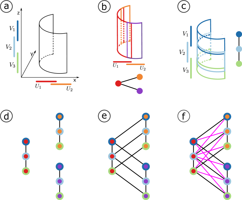
Figure 2: Illustration of Algorithm 1. (a) The space ${{\mathbb{X}}}$ is a half-cylinder in $\mathbb{R}^{3}$ with height along the $z$-axis. We consider $f=x$ and $g=z$. (b) Cover $\mathcal{U}=\{U_{1},U_{2}\}$ of $f({{\mathbb{X}}})$, path-connected pullback cover elements shown in red (for $U_{1}$), and in orange and purple (for $U_{2}$), and the mapper $M(f,\mathcal{U})$. (c) Cover $\mathcal{V}=\{V_{1},V_{2},V_{3}\}$ of $g({{\mathbb{X}}})$, corresponding path-connected pullback cover elements (in dark blue, sky blue, green), and the mapper $M(g,\mathcal{V})$. The composite cover $\mathcal{W}$ consists of 9 path-connected cover elements determined by the intersection of each element of $f^{*}(\mathcal{U})$ (in red, orange, and purple) with each element of $g^{*}(\mathcal{V})$ (dark blue, sky blue, and green). The corresponding vertices in the composite mapper are shown with these pairs of colors. (d) The mapper composition $M$ after the STITCH phase of Algorithm 1. (e) $M$ after the first stage of FIX phase (before running COMPLETE). $M$ is still $1$-dimensional at this stage. (f) The final composite mapper $S(M(f,\mathcal{U}),M(g,\mathcal{V}))$ after the COMPLETE phase, which adds the four tetrahedra (indicated by the pink diagonals) after adding the corresponding triangles which are their faces.

5 Proof of Theorem 3.1

The following proof for Theorem 3.1 shows that the composition of two univariate mappers is equivalent to the mapper directly constructed from a bivariate function encoding both filter functions. The proof follows directly from properties of continuous functions and connected sets.

Proof

Given a pair of filter functions $f,g:{{\mathbb{X}}}\to{{\mathbb{R}}}$ equipped with covers of their images $\mathcal{U}=\{U_{i}\}$ and $\mathcal{V}=\{V_{j}\}$, respectively, we define $h=(f,g):{{\mathbb{X}}}\to{{\mathbb{R}}}^{2}$. The pullback cover $\overline{\mathcal{W}}=h^{*}(\mathcal{U}\times\mathcal{V})$ is constructed from a cover of the image $h({{\mathbb{X}}})$ in the traditional manner. That is, the nerve of $\overline{\mathcal{W}}$ gives the traditional bivariate mapper.

Recall in Definition 1 that $\mathcal{W}$ is the path-connected components of the set $\{U^{\prime}\cap V^{\prime}\mid\forall U^{\prime}\in f^{*}(\mathcal{U}),\forall V^{\prime}\in g^{*}(\mathcal{V}),U^{\prime}\cap V^{\prime}\neq\emptyset\}$. This proof will show that $\mathcal{W}$ is equivalent to $\overline{\mathcal{W}}$.

First, we show that $\overline{\mathcal{W}}\subseteq\mathcal{W}$. Let $W\in\overline{\mathcal{W}}$ be any path-connected cover element of ${{\mathbb{X}}}$. By definition of the mapper and the refinement, we have $W\subseteq\overline{W_{i}}$ for some $\overline{W_{i}}=h^{-1}(U_{i}\times V_{j})$, $U_{i}\in\mathcal{U}$ and $V_{j}\in\mathcal{V}$. Thus, $h(W)\subseteq U_{i}\times V_{j}$. Note that $\overline{W_{i}}$ is not necessarily path-connected.

$h(W)$ can be further projected along the two filter functions such that $f(W)\subseteq U_{i}$ and $g(W)\subseteq V_{j}$. Hence, $W\subseteq f^{-1}(U_{i})$ and $W\subseteq g^{-1}(V_{j})$. Therefore, $W\subseteq f^{-1}(U_{i})\cap g^{-1}(V_{j})$. Since $W$ is path-connected, it must be the intersection of path-connected components from $f^{-1}(U_{i})$ and $g^{-1}(V_{j})$, respectively. That is, we must have $W=U^{\prime}\cap V^{\prime}$ for some path-connected components $U^{\prime}\in f^{-1}(U_{i})$ and $V^{\prime}\in g^{-1}(V_{j})$. Therefore, $W\in\mathcal{W}$; thus $\overline{\mathcal{W}}\subseteq\mathcal{W}$.

Second, we consider the cover $\mathcal{W}$ of ${{\mathbb{X}}}$ used to construct $S(M(f,\mathcal{U}),M(g,\mathcal{V}))$. We show that $\mathcal{W}\subseteq\overline{\mathcal{W}}$. Take a path-connected element $W\in\mathcal{W}$. By definition, $W\subseteq U^{\prime}\cap V^{\prime}$ for some path-connected $U^{\prime}\in f^{*}(\mathcal{U})$ and $V^{\prime}\in g^{*}(\mathcal{V})$. Thus, we have $W\subseteq U^{\prime}\in f^{-1}(U_{i})$ for some $U_{i}\in\mathcal{U}$ and similarly $W\subseteq V^{\prime}\in g^{-1}(V_{j})$ for some $V_{j}\in\mathcal{V}$. Thus, we have $f(W)\subseteq U_{i}$ and $g(W)\subseteq V_{j}$. It follows that $h(W)\subseteq U_{i}\times V_{j}$, and therefore, $W\subseteq h^{-1}(U_{i}\times V_{j})$.

This observation shows that $\overline{\mathcal{W}}$ and $\mathcal{W}$ are equivalent. Since both constructions of the mapper derive from the same cover, the resulting mappers must be equivalent.

6 Quantifying Topological Gains

Theorem 3.1 and Algorithm 1 inspire us to think about ways to quantify structural differences between a bivariate mapper and its corresponding univariate mappers. Moving from theory to practice, we consider three measures that quantify topological gains during the stitching process using homology or entropy. These measures are straightforward to compute, and use only information within each interval set from the STITCH phase of the composition algorithm. We aim to give simple quantitative measures describing the change in information content from a univariate mapper construction to a bivariate mapper construction. Although these measures do not capture the complete connectivity information across interval sets, they provide a quantitative assessment of the stitching process both globally and locally.

Notations. Before introducing these measures, we first introduce a few notations regarding mappers and mapper graphs restricted to interval sets. Given mappers $K_{f}:=M(f,\mathcal{U})$ and $K_{(f,g)}:=M((f,g),\mathcal{U}\times\mathcal{V})$, let $K_{f}(U_{i})$ be the subcomplex of $K_{f}$ restricted to the interval $U_{i}\in\mathcal{U}$, and similarly let $K_{(f,g)}(U_{i})$ be the subcomplex of $K_{(f,g)}$ restricted to the interval $U_{i}$.

We consider two types of restrictions. We construct interior subcomplexes $\mathring{K}_{f}(U_{i})$ by considering the subcomplexes of $K_{f}$ induced by vertices $x\in K_{f}$ whose function values $f(x)$ fall in the interval $U_{i}$. We also construct boundary subcomplexes $\overline{K}_{f}(U_{i})$ by considering all $\sigma\in\mathring{K}_{f}(U_{i})$ and their cofaces. Recall the star of a simplex in a simplicial complex $K$ consists of all its cofaces in $K$, $\mathrm{St}(\sigma)=\{\tau\in K\mid\sigma\leq\tau\}$. Then we have $\overline{K}_{f}(U_{i})=\{\mathrm{St}(\sigma)\mid\sigma\in\mathring{K}_{f}(U_{i})\}$. Similarly, we define $\mathring{K}_{(f,g)}(U_{i})$ and $\overline{K}_{(f,g)}(U_{i})$. If $K_{f}$ and $K_{(f,g)}$ are replaced by their 1-dimensional skeletons (referred to as their mapper graphs) denoted as $G_{f}$ and $G_{(f,g)}$, respectively, then we speak of interior subgraphs $\mathring{G}_{f}(U_{i})$ and boundary subgraphs $\overline{G}_{f}(U_{i})$ accordingly.

Both localized homological difference (Sect. 6.1) and local relative Euler characteristics (Sect. 6.2) are applicable to the mapper subcomplexes and mapper subgraphs, whereas the localized entropy differences (Sect. 6.3) are applicable only to the mapper subgraphs.

6.1 Localized Homological Difference

The localized homological difference ($\mathtt{LHD}$) compares the Betti numbers for each interval set between the two mapper constructions. This measure bears a weak resemblance to the approach taken by Edelsbrunner et al. EdelsbrunnerHarerNatarajan2004 , where local and global comparison measures are introduced for a pair of real-valued functions defined on a common domain; in particular, such measures can be related to the set of critical points from one function to the level sets of the other.

Intuitively speaking, the $\mathtt{LHD}$ characterizes the homological information gain during the composition (stitching) process. Starting with a mapper $K_{f}$ associated with the first function $f$, $\mathtt{LHD}$ studies what happens within each interval set while stitching a mapper $K_{g}$ associated with the second function $g$. Let $\beta_{p}(K)$ denote the $p$-th Betti number of a simplicial complex $K$.

Definition 2 (Localized Homological Difference)

Let $K_{f}:=M(f,\mathcal{U})$ be the first mapper and $K_{g}:=M(g,\mathcal{V})$ the second. We define $\mathtt{LHD}_{p}$ as a vector that quantifies the amount of $p$-dimensional homological information gained by stitching the second mapper onto the first one within each interval set $U_{i}\in\mathcal{U}$. That is, we define localized homology (LH) vectors $\beta_{p}^{f}$ and $\beta_{p}^{(f,g)}$ to encode homological information associated with each mapper subcomplex and compute their difference (suppose $|\mathcal{U}|=k$),

$$\beta_{p}^{f}=\left(\beta_{p}(K_{f}(U_{1}),\beta_{p}(K_{f}(U_{2}),\dots,\beta_{p}(K_{f}(U_{k}))\right),$$ (1)

$$\beta_{p}^{(f,g)}=\left(\beta_{p}(K_{(f,g)}(U_{1})),\beta_{p}(K_{(f,g)}(U_{2})),\dots,\beta_{p}(K_{(f,g)}(U_{k}))\right),$$ (2)

$$\mathtt{LHD}_{p}\left(K_{f},K_{(f,g)}\right)=\beta_{p}^{(f,g)}-\beta_{p}^{f}.$$ (3)

Here, $K_{f}(U_{i})$ and $K_{(f,g)}(U_{i})$ represent either interior or boundary subcomplexes.

Example 1 below demonstrates the $\mathtt{LHD}$ calculation for $p=1$ on a cylinder, using interior subcomplexes. Consider a cylinder embedded in a 3-dimensional space centered on the origin with a circle along the $x$-$y$ plane and the tube rising along the $z$-axis. Suppose we have three filter functions that represent the projection along the $x$, $y$, and $z$ axes, respectively. For simplicity, let us denote these filter functions as $x$, $y$, and $z$. The cover of each filter function is made of three equal length intervals with small overlaps spanning the range. Clearly, the images of filter functions $x$ and $y$ are nearly identical whereas that of $z$ is distinct. Let $K_{x}:=M(x,\mathcal{U})$ and $K_{z}:=M(z,\mathcal{V})$ denote the univariate mappers associated with filter functions $x$ and $z$, respectively. Also let $K_{(x,z)}:=M((x,z),\mathcal{U}\times\mathcal{V})$ be a bivariate mapper.

Example 1 ($\mathtt{LHD}_{1}$ on a cylinder)

$$\mathtt{LHD}_{1}\left(K_{x},K_{(x,z)}\right)=\begin{pmatrix}0-0\\ 0-0\\ 0-0\end{pmatrix}=\begin{pmatrix}0\\ 0\\ 0\end{pmatrix}$$

$$\mathtt{LHD}_{1}\left(K_{z},K_{(x,z)})\right)=\begin{pmatrix}1-0\\ 1-0\\ 1-0\end{pmatrix}=\begin{pmatrix}1\\ 1\\ 1\end{pmatrix}$$

To illustrate this example, consider the first interval set of the $x$ projection. $K_{x}$ has 1 vertex in $U_{1}\in\mathcal{U}$. $K_{(x,z)}$ restricted to $U_{1}$ then consists of a line of 3 vertices with 2 edges. Thus, for the first entry in $\mathtt{LHD}_{1}$, we have

$$\beta_{1}\left(K_{(x,z)}(U_{1}))-\beta_{1}(K_{x}(U_{1})\right)=0-0=0.$$

In contrast, the first interval set of $K_{z}$ contains 1 vertex, whereas $K_{(x,z)}$ within the same interval set contains a loop. Thus, for the first interval $V_{1}\in\mathcal{V}$,

$$\beta_{1}\left(K_{(x,z)}(V_{1}))-\beta_{1}(K_{z}(V_{1})\right)=1-0=1.$$

This example shows that more homological information is gained with respect to the first homology class by stitching $K_{x}$ (i.e., the mapper of filter function $x$) to $K_{z}$ than by stitching $K_{z}$ (i.e., the mapper of the filter function $z$) to $K_{x}$.

These $\mathtt{LHD}$ vectors have some interesting properties. For instance, we know that $\mathtt{LHD}_{0}=0$ when stitching the mapper $K_{x}$ to $K_{z}$, since including more filter functions will not split any path-connected components; otherwise, they would have been represented by a cover element of the filter function $z$ in the univariate mapper $K_{z}$ already. Additionally, $\mathtt{LHD}$ can be shown to be always nonnegative.

6.2 Local Relative Euler Characteristic

The local homology (LH) vectors can be summarized with the local relative Euler characteristic ($\mathtt{LREC}$) by computing the Euler characteristic restricted to each interval set, that is, the alternating sums of each homology class vector. Let $\chi(K)$ denote the Euler characteristic of a simplicial complex $K$.

Definition 3 (Local Relative Euler Characteristic)

Given a pair of mappers $K_{f}:=M(f,\mathcal{U})$ and $K_{g}=M(g,\mathcal{V})$, we define $\mathtt{LREC}$ as a vector that captures the extent to which $K_{g}$ effects the Euler characteristic within each interval set $U_{i}\in\mathcal{U}$ by stitching $K_{g}$ with $K_{f}$. That is, we define Euler characteristic vectors for $K_{f}$ and $K_{(f,g)}$ and compute their difference,

$$\chi^{f}=\left(\chi(K_{f}(U_{1})),\chi(K_{f}(U_{2})),\dots,\chi(K_{f}(U_{k}))\right),$$ (4)

$$\chi^{(f,g)}=\left(\chi(K_{(f,g)}(U_{1})),\chi(K_{(f,g)}(U_{2})),\dots,\chi(K_{(f,g)}(U_{k}))\right),$$ (5)

$$\mathtt{LREC}\left(K_{f},K_{(f,g)}\right)=\chi^{(f,g)}-\chi^{f}.$$ (6)

Example 2 below demonstrates the $\mathtt{LREC}$ calculation on the cylinder from Example 1.

Example 2 ($\mathtt{LREC}$ on a cylinder)

$$\mathtt{LREC}\left(K_{x},K_{(x,z)}\right)=\begin{pmatrix}1-1\\ 2-2\\ 1-1\end{pmatrix}=\begin{pmatrix}0\\ 0\\ 0\end{pmatrix}$$

$$\mathtt{LREC}\left(K_{z},K_{(x,z)}\right)=\begin{pmatrix}0-1\\ 0-1\\ 0-1\end{pmatrix}=\begin{pmatrix}-1\\ -1\\ -1\end{pmatrix}$$

As before, we illustrate this computation on a single interval set. First, consider the first interval set $U_{1}$ of the $x$ projection. $K_{x}$ has one vertex in $U_{1}$ (based on its corresponding interior subcomplex), so $\chi(K_{x}(U_{1}))=1$. $K_{(x,z)}$ restricted to the interval $U_{1}$ contains a line of 3 vertices with 2 edges, so $\chi(K_{(x,z)}(U_{1}))=3-2=1$. Thus, for the first entry in $\mathtt{LREC}$, we have

$$\chi(K_{(x,z)}(U_{1}))-\chi(K_{x}(U_{1}))=1-1=0.$$

In contrast, the first interval set of $K_{z}$ contains 1 vertex, that is $\chi(K_{z}(V_{1}))=1$; whereas $K_{(x,z)}$ within the same interval set contains a loop, that is, $\chi(K_{(x,z)}(V_{1}))=0$. Thus, for $V_{1}\in\mathcal{V}$,

$$\chi(K_{(x,z)}(V_{1}))-\chi(K_{z}(V_{1}))=0-1=-1.$$

However, the $\mathtt{LREC}$ being negative does not necessarily mean that the topological information has decreased. The Euler characteristic does not scale with the expected information change in an intuitive way, and so $\mathtt{LREC}$ may be a less interpretable measurement in comparison with $\mathtt{LHD}$.

6.3 Localized Entropy Differences

Finally, the localized entropy difference (LED) compares the graph entropy for each interval set between two mapper graphs. Graph entropy was introduced Rashevsky1955 ; Trucco1956 to measure the structural complexity of a graph, where it was originally referred to as the topological information content Rashevsky1955 of a graph. This is fitting for our purpose since we are interested in measuring the change of topological information content from a univariate mapper graph to a bivariate mapper graph. A number of graph entropy measures exist, see the survey by Dehmer and Mowshowitz DehmerMowshowitz2011 . We generalize and implement two of them in our visualization tool, although our framework is easily extendable to other entropy measures. For the remainder of this section, mapper graphs $G_{f}$ and $G_{(f,g)}$ represent the 1-skeletons of mappers $K_{f}:=M(f,\mathcal{U})$ and $K_{(f,g)}:=M((f,g),\mathcal{U}\times\mathcal{V})$, respectively.

Definition 4 (Localized Entropy Difference)

Given a pair of mapper graphs $G_{f}$ and $G_{(f,g)}$, we define $\mathtt{LED}$ as a vector that captures the extent to which $G_{g}$ affects the graph entropy within each interval set $U_{i}\in\mathcal{U}$. That is, we define localized entropy (LE) vectors for $G_{f}$ and $G_{(f,g)}$ and compute their difference,

$$H^{f}=\left(H(G_{f}(U_{1})),H(G_{f}(U_{2})),\dots,H(G_{f}(U_{k}))\right),$$ (7)

$$H^{(f,g)}=\left(H(G_{(f,g)}(U_{1})),H(G_{(f,g)}(U_{2})),\dots,H(G_{(f,g)}(U_{k}))\right),$$ (8)

$$\mathtt{LED}\left(G_{f},G_{\left(f,g\right)}\right)=H^{(f,g)}-H^{f}.$$ (9)

Here, $G_{f}(U_{i})$ and $G_{\left(f,g\right)}(U_{i})$ can be either interior or boundary mapper subgraphs. $H$ represents a certain notion of entropy. We introduce two types of LEDs, based on distance matrices and adjacency matrices, respectively.

Graph entropy based on the distance matrix. For an unweighted connected graph $G$, Bonchev and Trinajstić BonchevTrinajstic1977 introduced an entropy measure based on its graph distance matrix $D$. This measure originates from a notion in information theory called the information content (i.e., Shannon entropy) of a system.

Assume a system $S$ contains $N$ elements. Consider all the $N$ elements are partitioned into $m$ groups, and $N_{i}$ is the number of elements in the $i$-th group. We define the probability $p_{i}$ for a randomly selected element of $S$ to be found in the $i$-th group as $p_{i}=\frac{N_{i}}{N}$. Specifically, we work with the mean information content of one element of the system, defined by Shannon’s relation

$$H(S)=-\Sigma_{i=1}^{m}p_{i}\log{p_{i}}.$$ (10)

To apply Eq. 10 to the setting of a graph $G$ with $N$ vertices and introduce an information measure on its distance matrix $D$, we consider all $N^{2}$ matrix elements in $D$ as elements of a system. Since $G$ is an unweighted graph, the distance of a value $i$ (where $0\leq i\leq N-1$) appears $2k_{i}$ times in $D$. Let $m$ be the highest value of $i$, which equals the diameter of the graph. Then a total of $N^{2}$ matrix elements are partitioned into $m\text{+}1$ groups, which correspond to distances valued at $\{0,1,\dots,m\}$ respectively, where the value of $0$ shows up $N$ times. We associate each group with the probability for a randomly chosen distance to be in the $i$-th group. That is, $p_{i}=\frac{2k_{i}}{N^{2}}$ and $p_{0}=\frac{N}{N^{2}}=\frac{1}{N}$. Applying Eq. 10 to $m\text{+}1$ groups, the mean information on distances of a graph $G$ is defined as (BonchevTrinajstic1977, , Eq. (8))

$$H_{D}(G)=-\frac{1}{N}\log(\frac{1}{N})-\Sigma_{i=1}^{m}\frac{2k_{i}}{N^{2}}\log(\frac{2k_{i}}{N^{2}}).$$ (11)

In this paper, we generalize Eq. 11 to graphs with multiple connected components by considering $\infty$ as an additional possible value in the distance matrix $D$. That is, we define $p_{\infty}=\frac{2k_{\infty}}{N^{2}}$, where $2k_{\infty}$ is the number of times a value $\infty$ appears in $D$. Therefore, for a graph $G$ whose matrix $D$ might contain $\infty$ (that is, $G$ contains multiple connected components), we apply Eq. 12 with $m\text{+}2$ groups to define a mean entropy on distance,

$$H_{D}(G)=-\frac{1}{N}\log(\frac{1}{N})-\Sigma_{i=1}^{m}\frac{2k_{i}}{N^{2}}\log(\frac{2k_{i}}{N^{2}})-\frac{2k_{\infty}}{N^{2}}\log(\frac{2k_{\infty}}{N^{2}}).$$ (12)

Based on Eq. 12, we define $\mathtt{LED}$ based on distances as

$$\mathtt{LED}_{D}\left(G_{f},G_{(f,g)}\right)=H_{D}^{(f,g)}-H_{D}^{f}.$$ (13)

Intuitively speaking, $H_{D}(G)$ captures the information on the distribution of distances in the graph; it has been shown to be useful experimentally in studying the branching of graphs having different numbers of vertices BonchevTrinajstic1977 . Therefore, $\mathtt{LED}_{D}$ quantifies changes in branching structures moving from a univariate to a bivariate mapper graph.

Graph entropy based on the adjacency matrix. Mackenzie Mackenzie1966 proposed an entropy based on an adjacency matrix, which was employed by Sen et al. SenChuParhi2019 to study brain networks. For a weighted graph $G$, let $w_{ij}$ be the weight of edge $e_{ij}$ between vertices $v_{i}$ and $v_{j}$. Let $W=\Sigma_{e_{ij}\in E}(w_{ij})$ be the total edge weight. The probability of correlation between $v_{i}$ and $v_{j}$ is defined (SenChuParhi2019, , Eq. 5) as

$$q_{ij}=\begin{cases}\frac{w_{ij}}{W}&\text{when }i\neq j\text{, and }\\ 0&\text{when }i=j.\end{cases}$$

The mean entropy on adjacency is then defined as (SenChuParhi2019, , Eq. 6)

$$H_{A}(G)=-\Sigma_{e_{ij}\in E}\left(q_{ij}\log(q_{ij})\right).$$ (14)

We extend Eq. 14 to handle mapper subgraphs that are not necessarily connected by considering $q_{ij}=0$ when $v_{i}$ and $v_{j}$ belong to different connected components of $G$. Based on Eq. 14, we define $\mathtt{LED}$ based on adjacencies as

$$\mathtt{LED}_{A}\left(G_{f},G_{(f,g)}\right)=H_{A}^{(f,g)}-H_{A}^{f}.$$ (15)

Intuitively, $H_{A}(G)$ captures the centrality property of a graph: it varies inversely with respect to the structural centrality of $G$, that is, $H_{A}(G)$ increases as the graph becomes decentralized Mackenzie1966 . It can be used to compare a pair of graphs of different sizes, where a graph with a smaller entropy indicates more centrality thus less randomness SenChuParhi2019 in its structure. Therefore, $\mathtt{LED}_{A}$ quantifies changes in centrality moving from a univariate to a bivariate mapper graph.

Remarks. Finally, we note that a number of entropy measures are defined for simplicial complexes (e.g., DantchevIvrissimtzis2017 ), which may be applicable to mappers (not just mapper graphs). This is left for future work.

7 Visualizing Topological Gains

We provide a tool that visualizes topological gains during the stitching process. We experiment with two synthetic 2- or 3-dimensional point cloud datasets together with four classic datasets in machine learning, the Boston Housing dataset, the Iris dataset, the Breast Cancer dataset, and the Wine Quality dataset, some of which are available via the UCI Machine Learning Repository DuaGraff2017 . We also explore two real-world datasets, a phenomics dataset referred to as the KS/NE dataset and a breast cancer dataset referred to as the NKI dataset. For each dataset ${{\mathbb{X}}}$, we compare mapper graphs $G_{f}$ and $G_{(f,g)}$ constructed based on a pair of variables $f,g:{{\mathbb{X}}}\to{{\mathbb{R}}}$. We implement localized homological differences in dimensions 0 and 1 (denoted as $\mathtt{LHD}_{0}$ and $\mathtt{LHD}_{1}$), as well as localized entropy differences based on distances ($\mathtt{LED}_{D}$) and adjacencies ($\mathtt{LED}_{A}$), respectively.

Implementation details. We implement the tool using HTML/CSS/JavaScript stack with D3.js and JQuery libraries. It interfaces with a Python backend using a Flask-based server. The tool is an extension of Mapper Interactive ZhouChalapathiRathore2021 , which is an extendable and interactive toolbox for the visual exploration of high-dimensional data using the mapper algorithm. In particular, Mapper Interactive uses an accelerated modification of KeplerMapper VeenSaulEargle2019 to compute mapper graphs in a scalable way.

7.1 Visualization Interface

We begin with an example of a 2-dimensional point cloud ${{\mathbb{X}}}=\{(x_{i},y_{i})\}$ containing two nested circles in Fig. 3a to illustrate our main visualization interface. The mapper graph parameters are $n=7$, $p=5\%$. The two filter functions are chosen to be the $x$- and $y$-coordinates of the points, $x,y:{{\mathbb{X}}}\to{{\mathbb{R}}}$.

The main display is in the form of a mapper graph matrix, shown in Fig. 3 . As illustrated in Fig. 3, we construct univariate mapper graphs $G_{x}$ in (b) and $G_{y}$ in (e) for variables $x$ and $y$, respectively, that are placed along the diagonal of the mapper graph matrix. We construct bivariate mapper graphs $G_{(x,y)}$ in (c) and (d), respectively, which are shown off-diagonal. The mapper graphs are drawn with force-directed layouts. Nodes are colored by the index of intervals, where indices $1$ to $7$ correspond to the color light blue, dark blue, light green, dark green, pink, red, and orange, respectively.

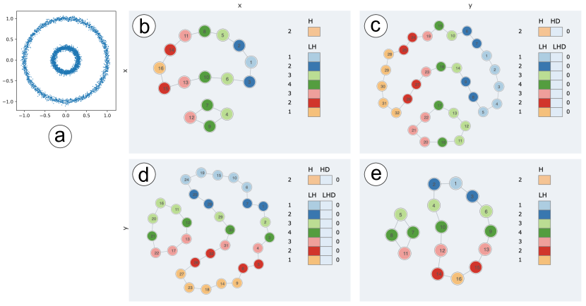
Figure 3: Two Circles dataset: the mapper graph matrix with $\mathtt{LHD}_{0}$. Graph nodes are colored by interval indices.

For each mapper graph, we report its associated 0-dimensional local homology (LH) vectors w.r.t. the interior mapper subgraphs. For instance, in Fig. 3e, the LH vector $\beta^{y}_{0}=(1,2,3,4,3,2,1)$ captures the number of connected components for the univariate mapper graph $G_{y}$ of variable $y$. The LH vector $\beta_{0}^{(x,y)}=(1,2,3,4,3,2,1)$ in Fig. 3d similarly captures the distribution of connected components for the bivariate mapper graph $G_{(x,y)}$ along the intervals for $y$. For each bivariate mapper graph $G_{(x,y)}$, we also report its localized homological difference ($\mathtt{LHD}_{0}$) w.r.t. $G_{x}$ and $G_{y}$, respectively. For instance, $\mathtt{LHD}_{0}(G_{x},G_{x,y})=0$ (Fig. 3c) and $\mathtt{LHD}_{0}(G_{y},G_{x,y})=0$ (Fig. 3d, due to symmetry).

In general, within a mapper graph matrix, univariate and bivariate mapper graphs are placed on and off the diagonal, respectively. For each mapper graph, the graph nodes are colored by the intervals they belong to: they are either colored by interval indices or by the value of a measure attached to each interval. The rectangle bars on the right of each mapper graph demonstrate the vector of either $\mathtt{LH}$ or $\mathtt{LE}$ restricted to the interval sets. They are either colored by interval indices (Fig. 3), or by a continuous colormap associated with the values of a chosen measure. For the bivariate mapper graphs, we also display $\mathtt{LHD}$/$\mathtt{LED}$ between the bivariate and univariate mapper graphs. Such differences are computed by subtracting the values of $\mathtt{LH}$ or $\mathtt{LE}$ in a univariate mapper graph from the values in a bivariate mapper graph on the same row.

By looking at $\mathtt{LHD}$ or $\mathtt{LED}$, we would know how much topological information is gained during the stitching process. In addition, by comparing the $\mathtt{LHD}$ or $\mathtt{LED}$ between two bivariate mapper graphs, we could identify the variables with high $\mathtt{LHD}$/$\mathtt{LED}$ values. Such a variable is considered to be more important than the other variables in terms of extracting topological information of a given point cloud. More detailed explanations of such comparisons will be provided in the examples below.

7.2 Cylinder

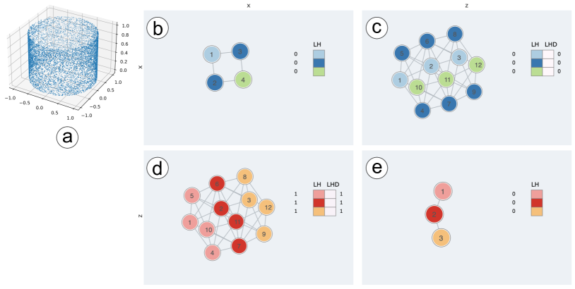
Figure 4: Cylinder dataset: the mapper graph matrix with $\mathtt{LHD}_{1}$. Graph nodes are colored by interval indices.

Our first example is to reproduce the result of Example 1 by generating a 3-dimensional cylinder point cloud ${{\mathbb{X}}}=\{(x_{i},y_{i},z_{i})\}$, where the $x$-, $y$-, and $z$-coordinates correspond to the three filter functions, respectively. The point cloud is shown in Fig. 4a. The mapper graph parameters are $n=3$, $p=15\%$. The two filter functions are chosen to be the $x$- and $z$- coordinates of the points, $x,z:{{\mathbb{X}}}\to{{\mathbb{R}}}$. The two univariate mapper graphs $G_{x}$ in Fig. 4b and $G_{z}$ in Fig. 4e for variables $x$ and $z$, respectively, are placed along the diagonal of Fig. 4. The bivariate mapper graphs $G_{(x,z)}$ are off diagonal in Fig. 4c and Fig. 4d, respectively.

For each mapper graph, we report its associated 1-dimensional local homology (LH) vectors w.r.t. the interior mapper subgraphs. The results confirm our previous computation in Sect. 6.1 that $\mathtt{LHD}_{1}$ increases when stitching $G_{x}$ to $G_{z}$, while $\mathtt{LHD}_{1}$ does not increase when stitching $G_{z}$ to $G_{x}$ (see Fig. 4d and Fig. 4c).

7.3 Sphere

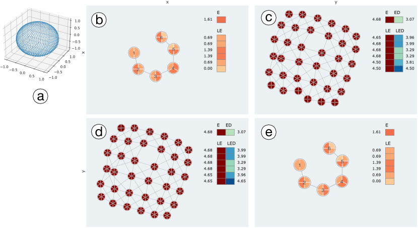
Figure 5: Sphere dataset: the mapper graph matrix with $\mathtt{LED}_{A}$. Graph nodes are colored by $LE$ measures restricted to the interval sets.

Our second example is a 3-dimensional point cloud sampled from the surface of a sphere (Fig. 5a). We again choose 2 of the 3 dimensions ($x$ and $y$) to compute the mapper graphs $G_{x}$ and $G_{y}$, as well as the boundary mapper subgraphs. The mapper parameters are $n=6$, $p=15\%$. In this example, we observe the information content, quantified by localized entropy difference (LED) based on adjacencies ($\mathtt{LED}_{A}$), increases in the bivariate mapper graphs, especially for the intervals capturing the top and bottom of the sphere. For instance, the localized entropy (LE) vectors $H^{x}$, $H^{(x,y)}$, and their difference are shown in Fig. 5b and Fig. 5c, respectively, where

$$H^{x} =\begin{pmatrix}0.00,&0.69,&1.39,&1.39,&0.69,&0.69\end{pmatrix},$$

$$H^{(x,y)} =\begin{pmatrix}4.50,&4.50,&4.68,&4.68,&4.68,&4.65\end{pmatrix},$$

$$\mathtt{LED}_{A}(H^{x},H^{(x,y)}) =\begin{pmatrix}4.50,&3.81,&3.29,&3.29,&3.99,&3.96\end{pmatrix}.$$

In this example, LHD does not give much information in dimension 0 since $\beta^{x}_{0}=\beta^{(x,y)}_{0}=(1,1,1,1,1,1)$, hence giving $\mathtt{LHD}_{0}=0$.

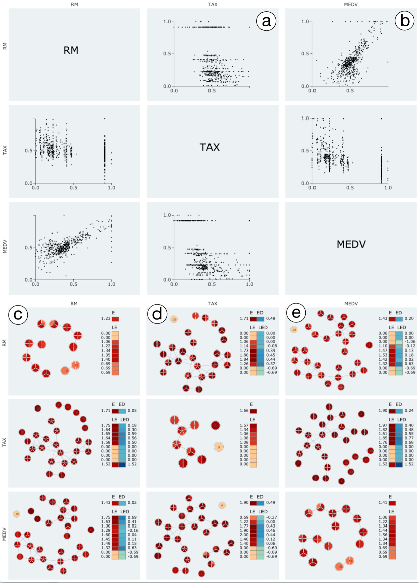
Figure 6: Boston Housing dataset. Top: the scatter plot matrix. Bottom: the mapper graph matrix with $\mathtt{LED}_{D}$; graph nodes are colored by $LE$ restricted to interval sets.

7.4 Boston Housing Dataset

Our third example is the classic Boston Housing dataset HarrisonRubinfeld1978 , which contains housing information in the Boston area collected by the U.S. Census Service. It contains 14 attributes per data point, including CRIM (per capita crime rate by town), RAD (index of accessibility to radial highways), and ZN (proportion of residential land zoned for lots over 25,000 sq. ft.). We chose three attributes as variables to compute the mapper graphs: RM, which is the average number of rooms per dwelling, TAX, which is the full-value property-tax rate per 10,000 dollars, and MEDV, which is the median value of owner-occupied homes in 1000’s of dollars, using mapper parameters $n=10$, $p=15\%$. We compute LED based on distances, denoted as $\mathtt{LED}_{D}$, for boundary mapper subgraphs. For instance, for variables RM and TAX (Fig. 6c, Fig. 6d),

$$H^{RM} =(0.69,0.69,0.69,1.4,1.35,1.34,1.22,1.06,0,0),$$

$$H^{(RM,TAX)} =(0,0,1.26,1.84,1.73,1.14,1.06,0,0),$$

$$\mathtt{LED}_{D}(H^{RM},H^{(RM,TAX)}) =(-0.69,-0.69,0.57,0.44,0.45,0.39,-0.08,0,0,0).$$

The mapper graph matrix complements the scatter plot matrix in Fig. 6. In particular, we observe globally that stitching the mapper graph $G_{TAX}$ to $G_{RM}$ has a higher global LED ($0.48$) in comparison to stitching $G_{MEDV}$ to $G_{RM}$ ($0.20$), which is aligned with the observation that RM vs. TAX are less correlated than RM vs. MEDV (see the scatter plots in Fig. 6a and Fig. 6b). Understanding the relation between topological gains and correlations among variables will be an interesting future direction.

7.5 Iris Dataset

Our fourth example is Fisher’s Iris dataset Fisher1936 , another classic dataset in machine learning. This dataset contains four attributes including the sepal length, sepal width, petal length, and petal width of each iris plant. We use all four attributes to compute the mapper graph matrix, with mapper parameters $n=10$, $p=30\%$. As shown in Fig. 7, we combine both the scatter plot matrix and the mapper graph matrix. We observe that stitching the mapper graph associated with sepal width to petal length has a higher global $\mathtt{LED}_{A}$ (Fig. 7c, $2.20$) than stitching petal width to petal length (Fig. 7d, $0.41$). Such a topological gain is also observed locally for boundary subgraphs. At the same time, petal length is shown to be more correlated to petal width than with sepal width (see Fig. 7b and Fig. 7a).

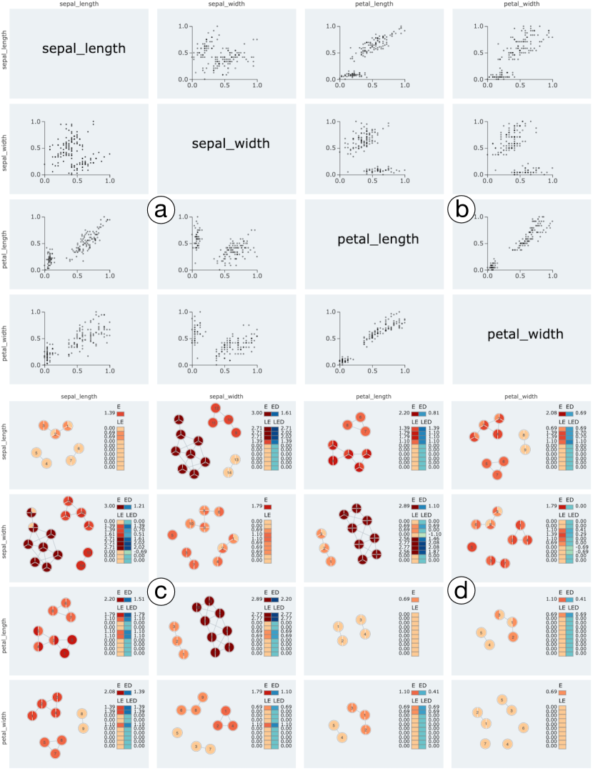
Figure 7: Iris dataset. Top: the scatter plot matrix. Bottom: the mapper graph matrix with $\mathtt{LED}_{A}$; graph nodes are colored by $LE$ restricted to interval sets.

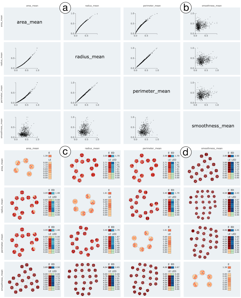
Figure 8: Breast Cancer dataset. Top: the scatter plot matrix. Bottom: the mapper graph matrix with $\mathtt{LED}_{A}$; graph nodes are colored by $LE$ restricted to interval sets.

7.6 Breast Cancer Wisconsin (Diagnostic) Dataset

Our fifth dataset describes characteristics of the cell nuclei present in the images of breast masses MangasarianStreetWolberg1995 ; StreetWolbergMangasarian1993 . We choose four variables from among ten real-valued features computed for each cell nucleus: area mean (mean area of the tumor), radius mean (mean of distances from the center to points on the perimeter), parameter mean (mean size of the core tumor), and smoothness mean (mean of local variation in radius lengths). We compute univariate and bivariate mapper graphs using boundary subgraphs, with parameters $n=8$, $p=20\%$. As shown in the scatter plot matrix (Fig. 8), area mean and radius mean are highly correlated, but area mean and smoothness mean are not. We observe that stitching the mapper graph of the smoothness mean to that of the area mean achieves a higher global and local $\mathtt{LED}_{A}$ than stitching radius mean with area mean (see Fig. 8d and Fig. 8c).

7.7 Wine Quality Dataset

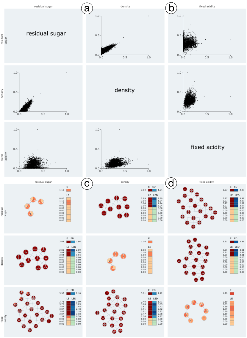
Figure 9: Wine Quality dataset. Top: the scatter plot matrix. Bottom: the mapper graph matrix with $\mathtt{LED}_{A}$; graph nodes are colored by $LE$ restricted to interval sets.

Our sixth dataset is the wine quality dataset, which is another classic machine learning dataset, and gives 11 variables describing wine quality based on physicochemical tests CerdeiraAlmeidaMatos2009 . We use 3 of these variables for our analysis: residual sugar, density, and fixed acidity. The scatter plot matrix shows that residual sugar and density are highly correlated (Fig. 9a), but residual sugar and fixed acidity are not (Fig. 9b). Complementarily, we see that stitching the mapper graph of fixed acidity to the mapper graph of residual sugar gives rise to higher $\mathtt{LED}_{A}$ globally and locally than stitching density with residual sugar (see Fig. 9d and Fig. 9c).

7.8 KS/NE dataset

We also explore a real-world phenomics dataset referred to as the KS/NE dataset and was first studied by Kamruzzaman et al. KamruzzamanKalyanaramanKrishnamoorthy2019 . It records daily measurements of maize plants that were cultivated in Kansas (KS) and Nebraska (NE). The columns consist of the genotype of each plant, the growth rate of each plant (growth_rate), a time measurement describing the days after planting (DAP), and 10 environmental variables including humidity, temperature, rainfall, solar radiation, etc. There are 400 rows, with each row corresponding to the daily record of a plant. We construct a 1D point cloud using growth_rate, and choose the variables DAP and humidity to compute the mapper graphs $G_{DAP}$, $G_{humidity}$, and $G_{(DAP,humidity)}$, as well as the boundary mapper subgraphs. The mapper parameters are $n=10$, $p=46\%$.

As shown in Fig. 10, we observe that the bivariate mapper graphs have positive $\mathtt{LED}_{A}$ both globally and locally, indicating the bivariate mapper graphs have more topological gains than the univariate mapper graphs. In particular, stitching $G_{humidity}$ to $G_{DAP}$ has a higher global $\mathtt{LED}_{A}$ compared with stitching $G_{DAP}$ to $G_{humidity}$ (see Fig. 10b and Fig. 10c), indicating that $humidity$ is a more important variable than $DAP$ for capturing the topological structure of the point cloud data. The scatter plot matrix Fig. 10a shows that the two variables are not correlated.

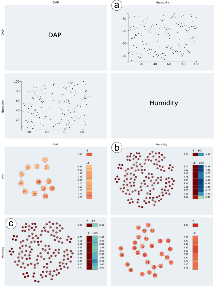
Figure 10: KS/NE dataset: Top: the scatter plot matrix. Bottom: the mapper graph matrix with $\mathtt{LED}_{A}$; graph nodes are colored by $LE$ restricted to interval sets.

7.9 NKI dataset

We explore another real-world dataset, the breast cancer dataset that provides prognosis and gene expression information of patients. This dataset is referred to as the NKI dataset Vant-VeerDaiVan-De-Vijver2002 , which was previously studied by Lum et al. LumSinghLehman2013 and Zhou et al. ZhouChalapathiRathore2021 to identify subgroups in breast cancer patients. It contains 272 rows, with each row corresponding to the information of a patient. The columns consist of 1554 gene expression levels, and variables of medical records or physiological measures such as event_death (whether a patient survived or not), survival_time, recurrence_time, etc. We construct the point cloud using the 1500 mostly varying genes, and choose the variable event_death together with the infinity norm ($L_{\infty}$) of the point cloud to compute the mapper graphs $G_{event\_death}$, $G_{L_{\infty}}$ and $G_{(event\_death,L_{\infty})}$, as well as the boundary mapper graphs. The mapper parameters are $n=18$, $p=68\%$.

As shown in Fig. 11, we observe that the bivariate mapper graphs have positive $\mathtt{LED}_{D}$ both globally and locally, indicating the bivariate mapper graphs have more topological gains than the univariate mapper graphs. In particular, stitching $G_{L_{\infty}}$ to $G_{event\_death}$ has a higher global $\mathtt{LED}_{D}$ compared with stitching $G_{event\_death}$ to $G_{L_{\infty}}$ (see Fig. 11b and Fig. 11c), indicating that $L_{\infty}$ is a more important variable than event_death for capturing the topological structure of the point cloud data. The scatter plot matrix Fig. 11a shows that the two variables are not correlated.

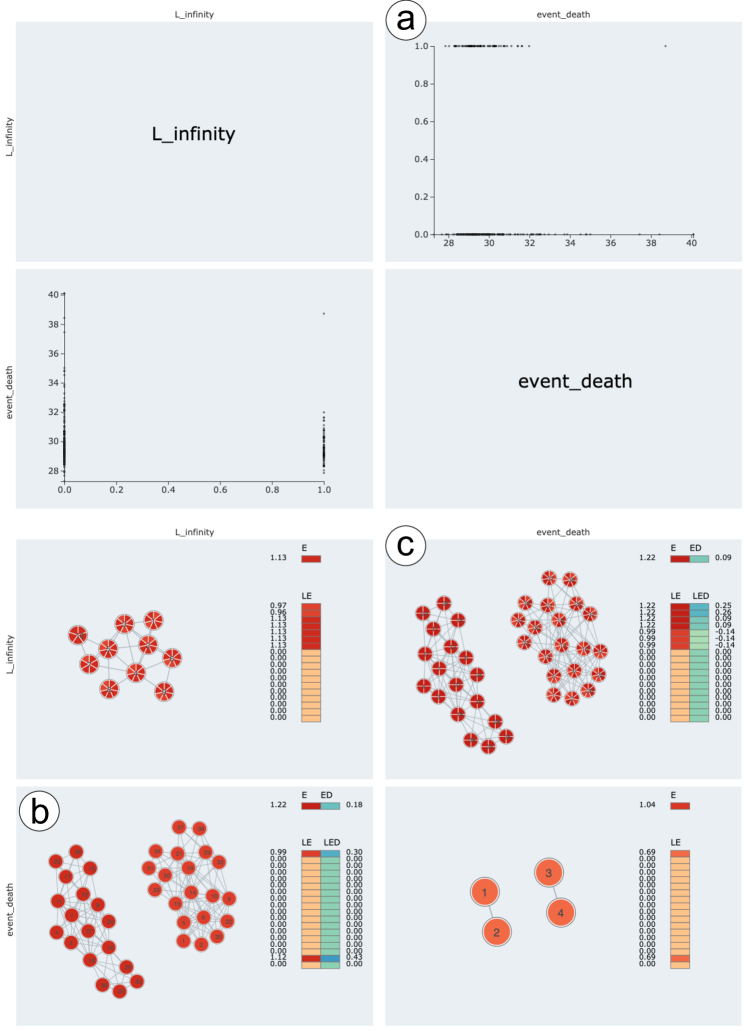
Figure 11: NKI dataset: Top: the scatter plot matrix. Bottom: the mapper graph matrix with $\mathtt{LED}_{D}$; graph nodes are colored by $LE$ restricted to interval sets.

8 Discussion

We study a method of stitching (composing) a pair of univariate mappers together into a bivariate mapper. By tracking the STITCH and FIX steps of the construction process, it is possible to quantify the relationship between filter functions. We further propose measures of topological gains that quantify the changes in topological content during the stitching process.

With such measures in hand, we return to our topological analogues of the stepwise regression Efroymson1960 and scatter plot matrix ElmqvistDragicevicFekete2008 , which help to navigate topological relationships among multiple filter functions. A method for stepwise stitching would produce a mapper with optimal topological information by iteratively building a multivariate mapper from topologically independent filter functions. A topological scatter plot matrix can reveal information about the filter functions such as topological dependencies and outliers by providing a visualization of the most information-rich filter functions. Our visualization tool provides a playground for such types of future work. Furthermore, based on various datasets analyzed in Sect. 7, we observe that stitching the mapper graphs of highly correlated variables typically gives rise to smaller changes in entropy ($\mathtt{LED}$) than stitching the mapper graphs of uncorrelated variables. Studying the relation between topological correlations (via mapper graphs) and statistical correlations will be an interesting future direction.

- (1) Alagappan, M.: From 5 to 13: Redefining the positions in basketball. MIT Sloan Sports Analytics Conference (2012)
- (2) Babu, A.: Zigzag coarsenings, mapper stability and gene-network analyses. Ph.D. thesis, Stanford University (2013)
- (3) Barral, V., Biasotti, S.: 3D shape retrieval and classification using multiple kernel learning on extended reeb graphs. The Visual Computer 30(11), 1247–1259 (2014)
- (4) Biasotti, S., Giorgi, D., Spagnuolo, M., Falcidieno, B.: Reeb graphs for shape analysis and applications. Theoretical Computer Science 392, 5–22 (2008)
- (5) Bonchev, D., Trinajstić, N.: Information theory, distance matrix, and molecular branching. The Journal of Chemical Physics 67(10), 4517–4533 (1977)
- (6) Brown, A., Bobrowski, O., Munch, E., Wang, B.: Probabilistic convergence and stability of random mapper graphs. Journal of Applied and Computational Topology 5, 99–140 (2021)
- (7) Carr, H., Duke, D.: Joint Contour Nets: Computation and properties. In: IEEE Pacific Visualization Symposium, pp. 161–168 (2013)
- (8) Carr, H., Duke, D.: Joint Contour Nets. IEEE Transactions on Visualization and Computer Graphics 20(8), 1100–1113 (2014)
- (9) Carriére, M., Oudot, S.: Structure and stability of the one-dimensional mapper. Foundations of Computational Mathematics 18(6), 1333–1396 (2018)
- (10) Cerdeira, A., Almeida, F., Matos, T., Reis, J.: Viticulture Commission of the Vinho Verde Region (CVRVV), Porto, Portugal (2009)
- (11) Chazal, F., Sun, J.: Gromov-Hausdorff approximation of filament structure using Reeb-type graph. Proceedings of the 13th Annual Symposium on Computational Geometry pp. 491–500 (2014)
- (12) Dantchev, S., Ivrissimtzis, I.: Simplicial complex entropy. In: M. Floater, T. Lyche, M.L. Mazure, K. Mørken, L. Schumaker (eds.) Mathematical Methods for Curves and Surfaces. MMCS 2016. Lecture Notes in Computer Science, vol. 10521. Springer (2017)
- (13) Dehmer, M., Mowshowitz, A.: A history of graph entropy measures. Information Sciences 181(57-78) (2011)
- (14) Dey, T.K., Mémoli, F., Wang, Y.: Mutiscale mapper: A framework for topological summarization of data and maps. Proceedings of the 27th annual ACM-SIAM symposium on Discrete algorithms pp. 997–1013 (2016)
- (15) Dey, T.K., Mémoli, F., Wang, Y.: Topological analysis of nerves, Reeb spaces, mappers, and multiscale mappers. In: B. Aronov, M.J. Katz (eds.) 33rd International Symposium on Computational Geometry, Leibniz International Proceedings in Informatics (LIPIcs), vol. 77, pp. 36:1–36:16. Schloss Dagstuhl–Leibniz-Zentrum fuer Informatik, Dagstuhl, Germany (2017)
- (16) Dua, D., Graff, C.: UCI machine learning repository. http://archive.ics.uci.edu/ml, University of California, Irvine, School of Information and Computer Sciences (2017)
- (17) Edelsbrunner, H., Harer, J.: Computational Topology: An Introduction. AMS, Providence, RI, USA (2010)
- (18) Edelsbrunner, H., Harer, J., Natarajan, V., Pascucci, V.: Local and global comparison of continuous functions. Proceedings of IEEE Conference on Visualization pp. 275–280 (2004)
- (19) Edelsbrunner, H., Harer, J., Patel, A.K.: Reeb spaces of piecewise linear mappings. In: Proceedings of the 24th Annual Symposium on Computational Geometry, pp. 242–250 (2008)
- (20) Efroymson, M.: Multiple regression analysis. In: A. Ralston, H.S. Wilf (eds.) Mathematical Methods for Digital Computers. Wiley, New York (1960)
- (21) Elmqvist, N., Dragicevic, P., Fekete, J.D.: Rolling the dice: Multidimensional visual exploration using scatterplot matrix navigation. IEEE Transactions on Visualization and Computer Graphics 14(6) (2008)
- (22) Ester, M., Kriegel, H.P., Sander, J., Xu, X.: A density-based algorithm for discovering clusters in large spatial databases with noise. Proceedings of the 2nd International Conference on Knowledge Discovery and Data Mining pp. 226–231 (1996)
- (23) Fisher, R.A.: The use of multiple measurements in taxonomic problems. Annals of Eugenics 7(2), 179–188 (1936)
- (24) Gasparovic, E., Gommel, M., Purvine, E., Sazdanovic, R., Wang, B., Wang, Y., Ziegelmeier, L.: A complete characterization of the one-dimensional intrinsic Čech persistence diagrams for metric graphs. In: E. Chambers, B. Fasy, L. Ziegelmeier (eds.) Research in Computational Topology, pp. 33–56. Springer International Publishing (2018)
- (25) Gundert, A., Szedlák, M.: Higher dimensional discrete Cheeger inequalities. Journal of Computational Geometry 6(2), 54–71 (2015)
- (26) Hajij, M., Assiri, B., Rosen, P.: Parallel mapper. In: Proceedings of the Future Technologies Conference, pp. 717–731. Springer (2020)
- (27) Harrison Jr, D., Rubinfeld, D.L.: Hedonic housing prices and the demand for clean air. Journal of environmental economics and management 5(1), 81–102 (1978)
- (28) Hilaga, M., Shinagawa, Y., Kohmura, T., Kunii, T.L.: Topology matching for fully automatic similarity estimation of 3D shapes. Proceedings of the 28th Annual Conference on Computer Graphics and Interactive Techniques pp. 203–212 (2001)
- (29) Hocking, R.R.: The analysis and selection of variables in linear regression. Biometrics 32 (1976)
- (30) Kamruzzaman, M., Kalyanaraman, A., Krishnamoorthy, B., Hey, S., Schnable, P.: Hyppo-X: A scalable exploratory framework for analyzing complex phenomics data. IEEE/ACM Transactions on Computational Biology and Bioinformatics (2019)
- (31) Lum, P.Y., Singh, G., Lehman, A., Ishkanov, T., Vejdemo-Johansson, M., Alagappan, M., Carlsson, J., Carlsson, G.: Extracting insights from the shape of complex data using topology. Scientific Reports 3(1236) (2013)
- (32) Mackenzie, K.D.: The information theoretic entropy function as a total expected participation index for communication network experiments. Psychometrika 31(2), 249–254 (1966)
- (33) Mangasarian, O., Street, W., Wolberg, W.: Breast cancer diagnosis and prognosis via linear programming. Operations Research 43(4), 570–577 (1995)
- (34) Müllner, D., Babu, A.: Python Mapper: An open-source toolchain for data exploration, analysis and visualization. http://danifold.net/mapper (2013)
- (35) Munch, E., Wang, B.: Convergence between categorical representations of Reeb space and mapper. In: S. Fekete, A. Lubiw (eds.) 32nd International Symposium on Computational Geometry, Leibniz International Proceedings in Informatics (LIPIcs), vol. 51, pp. 53:1–53:16. Schloss Dagstuhl–Leibniz-Zentrum fuer Informatik, Dagstuhl, Germany (2016)
- (36) Nicolau, M., Levine, A.J., Carlsson, G.: Topology based data analysis identifies a subgroup of breast cancers with a unique mutational profile and excellent survival. Proceedings of the National Academy of Sciences 108(17), 7265–7270 (2011)
- (37) Rashevsky, N.: Life information theory and topology. Bulletin of Mathematical Biophysics 17, 229–235 (1955)
- (38) Robles, A., Hajij, M., Rosen, P.: The shape of an image: A study of mapper on images. In: International Conference on Computer Vision Theory and Applications (VISAPP) (2018)
- (39) Saggar, M., Sporns, O., Gonzalez-Castillo, J., Bandettini, P.A., Carlsson, G., Glover, G., Reiss, A.L.: Towards a new approach to reveal dynamical organization of the brain using topological data analysis. Nature Communications 9(1399) (2018)
- (40) Sen, B., Chu, S.H., Parhi, K.K.: Ranking regions, edges and classifying tasks in functional brain graphs by sub-graph entropy. Scientific Reports 9(1), 1–20 (2019)
- (41) Singh, G., Mémoli, F., Carlsson, G.: Topological methods for the analysis of high dimensional data sets and 3D object recognition. Eurographics Symposium on Point-Based Graphics 22 (2007)
- (42) Street, W., Wolberg, W., Mangasarian, O.: Nuclear feature extraction for breast tumor diagnosis. IS&T/SPIE 1993 International Symposium on Electronic Imaging: Science and Technology 1905, 861–870 (1993)
- (43) Tauzin, G., Lupo, U., Tunstall, L., Pérez, J.B., Caorsi, M., Medina-Mardones, A., Dassatti, A., Hess, K.: giotto-tda: A topological data analysis toolkit for machine learning and data exploration. Journal of Machine Learning Research 22, 1–6 (2021)
- (44) The GUDHI Project: GUDHI User and Reference Manual. https://gudhi.inria.fr/doc/3.3.0/ (2020)
- (45) Trucco, E.: A note on the information content of graphs. Bulletin of Mathematical Biology 18(2), 129–135 (1956)
- (46) Van’t Veer, L.J., Dai, H., Van De Vijver, M.J., He, Y.D., Hart, A.A., Mao, M., Peterse, H.L., Van Der Kooy, K., Marton, M.J., Witteveen, A.T., et al.: Gene expression profiling predicts clinical outcome of breast cancer. nature 415(6871), 530–536 (2002)
- (47) van Veen, H.J., Saul, N., Eargle, D., Mangham, S.W.: Kepler Mapper: A flexible Python implementation of themapper algorithm. Journal of Open Source Software 4(42), 1315 (2019)
- (48) van Veen, H.J., Saul, N., Eargle, D., Mangham, S.W.: Kepler Mapper: A flexible Python implementation of themapper algorithm (version 1.3.3). Zenodo, http://doi.org/10.5281/zenodo.1054444 (2019)
- (49) Yan, L., Masood, T.B., Sridharamurthy, R., Rasheed, F., Natarajan, V., Hotz, I., Wang, B.: Scalar field comparison with topological descriptors: Properties and applications for scientific visualization. Computer Graphics Forum 40(3), 599–633 (2021)
- (50) Zhou, Y., Chalapathi, N., Rathore, A., Zhao, Y., Wang, B.: Mapper Interactive: A scalable, extendable, and interactive toolbox for the visual exploration of high-dimensional data. IEEE Pacific Visualization Symposium (2021)
- (51) Zhou, Y., Kamruzzaman, M., Schnable, P., Krishnamoorthy, B., Kalyanaraman, A., Wang, B.: Pheno-Mapper: An interactive toolbox for the visual exploration of phenomics data. In: ACM Conference on Bioinformatics, Computational Biology, and Health Informatics (ACM BCB) (2021)