Energy Spectrum of Thermalizing High Energy Decay Products in the Early Universe

Abstract

We revisit the Boltzmann equation governing the spectrum of energetic particles originating from the decay of massive progenitors during the process of thermalization. We assume that these decays occur when the background temperature $T$ is much less than the mass $M$ of the progenitor. We pay special attention to the IR cutoff provided by the thermal bath, and include the suppression resulting from the interference of multiple scattering reactions (LPM effect). We solve the resulting integral equation numerically, and construct an accurate analytical fit of the solutions.

1 Introduction

Energy injection into the primordial thermal plasma is an essential ingredient in various inflationary [1] and extended cosmology histories [2, 3], i.e. histories including an early era where the energy density of the universe was dominated by a fluid with an equation of state other than that of the standard radiation [4, 7, 5, 8, 9, 6]. A matter dominated phase at the end of inflation, or a late matter-dominated era due to some long-lived massive particle, are viable [10, 11], well-motivated, and extensively studied realizations of such cosmological histories. We will present our work with this context in mind, but our results will not depend on whether or not this extra contribution is dominant.

The energy injection process typically involves the decay of heavy, nonrelativistic particles into ultra-relativistic particles and the subsequent thermalization of these decay products. In this process the number density of the energetic particles grows, reducing the average energy of the individual particles to eventually match that of the thermal bath species. As long as the decay products have some gauge interactions the general behavior and chain of processes can be expected to be fairly independent of the details of the model [12], allowing one to make robust predictions of cosmological parameters, like the reheat temperature $T_{\scriptscriptstyle\rm RH}$ at the onset of radiation domination, and the rate of energy loss for the high energetic particles propagating through and interacting with the thermal bath.

We will see that the thermalization typically occurs at a time scale which is much shorter than the Hubble time. This means that the temperature of the bath can be taken to be constant during the thermalization of any one primary particle. As a result, during the epoch of energy injection the spectrum of non-thermal particles can be described by a universal function, whose shape only depends on the temperature and the initial injection energy scale, while the normalization depends on the number density and lifetime of the progenitor particles, along with the interaction strength involved in the thermalization process. These ultra-relativistic but non-thermal particles satisfy the same equation of state as thermal radiation; hence the thermalization does not affect the expansion history of the Universe. However, both before the decay and during the process of thermalization, this extra component can contribute to and affect the production of dark matter particles (or other long-lived or stable relics) [28, 9, 18, 24, 25, 22, 23, 12, 26, 27, 13, 14, 15, 16, 17, 19, 20, 21], the generation of the baryon asymmetry [29, 19, 20, 30, 31, 32], and other cosmological processes [65, 34, 35, 36, 37, 38]. Scenarios of dark matter production in extended cosmologies are particularly interesting in light of the shrinking of the viable thermal WIMP parameter space [42, 40, 43, 39, 41, 44, 46, 45].

An accurate description of the spectrum of non-thermal particles is therefore crucial for a reliable estimate of the rate of such non-thermal production processes. The main goal of this work is to calculate this spectrum in an easy to use form. We improve the treatment of refs.[12] by including the Landau-Pomeranchuk-Migdal (LPM) effect [47, 48], which slows down thermalization and thereby increases the density of non-thermal particles. Our result differs from that of refs.[22, 49, 23] in both shape and – by a numerical factor – in normalization. We consistently use the temperature of the thermal bath as IR regulator, and carefully distinguish between the most common thermalization processes and those that dominate the energy loss.

The rest of this article is organized as follows. In Sec. 2 we carefully formulate the problem. We first describe the basic framework, and the energy loss rate including the LPM effect. We then write down a Boltzmann equation for the spectrum, which we further reformulate in a form which is more easily solvable numerically. The numerical solution and an analytical approximation are described in Sec. 3, in addition to an example of how a spectrum of high-energy out-of-equilibrium particles affects the production of heavy stable relics. Finally, Sec. 4 contains a brief summary and the conclusions.

2 Formulation of the Problem

2.1 Basic Setup

To be specific we will focus on the decay of a heavy, relatively long-lived progenitor particle with mass $M$ into two ultra-relativistic particles whose masses are significantly smaller than the temperature of the thermal plasma; “long-lived” here means that the progenitors are not in thermal equilibrium when they decay. For the assumed two-body decay the injection spectrum is just a delta-function at $M/2$. Since the problem is linear, the final spectrum of non-thermal particles for any more complicated decay, or indeed for any other non-thermal injection spectrum, can be computed by simply convoluting our result with the assumed initial spectrum. We assume that both the thermal bath and the injected particles carry gauge charge. This is true in particular for all Standard Model (SM) particles, and for most of the particles predicted by its minimal supersymmetric extension.

Let us begin by presenting a general formulation of the the relevant cosmological history. We introduce a matter component of heavy particles of mass $M$, and number density $n_{\scriptscriptstyle\rm M}$, decaying with a width $\Gamma_{\scriptscriptstyle\rm M}$ into ultra-relativistic particles of initial energy $E_{\scriptscriptstyle\rm i}=M/2$. The evolution equation for the radiation and matter energy densities are then given by:

$$\frac{d\rho_{\scriptscriptstyle\rm M}}{dt}+3H\rho_{\scriptscriptstyle\rm M} = -\Gamma_{\scriptscriptstyle\rm M}\,\rho_{\scriptscriptstyle\rm M}\,;$$ (2.1a)

$$\frac{d\rho_{\scriptscriptstyle\rm R}}{dt}+4H\rho_{\scriptscriptstyle\rm R} = +\Gamma_{\scriptscriptstyle\rm M}\,\rho_{\scriptscriptstyle\rm M}\,.$$ (2.1b)

Here $H$ is the Hubble expansion rate and $t$ denotes the cosmological time of FLRW cosmology. $\rho_{\scriptscriptstyle\rm M}$ and $\rho_{\scriptscriptstyle\rm R}$ denote the energy density of the decaying matter component and the radiation component. For a given theory, the energy density as well as the number density of a fully thermalized radiation bath is determined completely by the temperature $T$ [54]:

$$\rho_{\scriptscriptstyle\rm R}^{\rm\scriptscriptstyle Th}(T) = \frac{\pi^{2}}{30}\,g_{*}\,T^{4}\,;$$ (2.2a)

$$n_{\scriptscriptstyle\rm R}^{\rm\scriptscriptstyle Th} = g_{\scriptscriptstyle\rm*n}\frac{\zeta(3)}{\pi^{2}}T^{3}\,,$$ (2.2b)

with $\zeta(3)=1.202$. Here $g_{*}$ and $g_{\scriptscriptstyle\rm*n}$ count the effective number of relativistic degrees of freedom (d.o.f.) contributing to the energy and number density, respectively. The temperature $T$ is usually also used to parameterize the evolution history of the universe. However, in our case the radiation component $\rho_{\scriptscriptstyle\rm R}$ is to be understood as consisting of the thermal radiation bath $\rho_{\scriptscriptstyle\rm R}^{\rm\scriptscriptstyle Th}$ and the (typically sub-dominant) non-thermal radiation component resulting from the decays of progenitor particles prior to thermalization. Note that both components are redshifted in the same manner.

We are yet to determine the interplay between $\rho_{\scriptscriptstyle\rm R}^{\rm\scriptscriptstyle Th}$ and $\rho_{\scriptscriptstyle\rm R}$, and so equations (2.1) are not sufficient for the study of the process of thermalization. In fact, we will now show that the relatively short timescale needed to thermalize energetic particles allows us to disregard the Hubble expansion and to treat the background FLRW universe as static when analyzing the thermalization process.

2.2 The Thermalization of Energetic Particles

The process of thermalization in a (quasi-)static background has been extensively studied in the literature [12, 49, 56, 22, 23]. For a convenient formulation based on the parameters of the extended cosmological history, we will mainly rely on the results from [22, 23] to describe the energy loss of energetic particles (with energy $E\gg T$) through interactions with the much more abundant particles in the thermal plasma.

Most notably, it is known that $2\rightarrow 2$ scattering processes do not determine this energy loss, even though they are of leading order in coupling constants. The reason is that elastic processes either suffer from a suppressed rate, or offer a small momentum transfer between the high-energy states and the thermal bath. These processes can reduce the energy of the incoming particle significantly only if there is large momentum exchange through the single propagator, which implies that the exchanged particle is far off-shell, leading to a power-suppressed scattering amplitude. On the other hand, the infrared divergence corresponding to the forward scattering of the high-energy particles off the thermal bath and involving massless intermediate bosons provides a significant interaction rate for processes with small momentum exchange. In the more complete picture of thermal field theory of a bath of temperature $T$, this IR divergence is regulated, as the intermediate state picks up an induced thermal mass:

$$m_{\scriptscriptstyle\rm th}\sim\alpha^{1/2}T,$$ (2.3)

where $\alpha$ is the coupling strength of the relevant gauge interaction. The thermally regulated rate of soft elastic scatterings is then

$$\Gamma_{\scriptscriptstyle\rm el}\sim\tilde{g}_{*}\alpha T\,.$$ (2.4)

The factor of $\tilde{g}_{*}$ is introduced to account for the number degrees of freedom in the thermal plasma that couple to the given interaction of strength $\alpha$. This implies that soft two-to-two processes, which on average occur in intervals of $\delta t_{\scriptscriptstyle\rm el}=\Gamma_{\scriptscriptstyle\rm el}^{-1}$, allow for a momentum transfer

$$\delta k_{\scriptscriptstyle\rm el}\sim m_{\scriptscriptstyle\rm th}\sim\alpha^{1/2}T\,.$$ (2.5)

In contrast, $2\rightarrow 3$ reactions, despite requiring an additional vertex insertion, can lead to a large energy loss without large momentum flow through any propagator, if the energetic particle splits into two nearly collinear particles either before or after exchanging momentum with the thermal plasma. As first noted in [57], such “splitting processes” therefore dominate the rate of energy loss [12, 22]. This energy loss will be significant only if the daughter particle produced in the splitting has energies well above $T$. It is important to note that the splitting process also increases the number of non-thermal particles, which is crucial for thermalization both with and without a preexisting thermal bath. A cascade of such reactions will therefore eventually turn an initially injected particle with energy $E_{\scriptscriptstyle\rm i}$ into $\sim E_{\scriptscriptstyle\rm i}/T$ particles, each with energy $\sim T$, which just become part of the thermal background described by eq.(2.2b). As mentioned before, $2\rightarrow 3$ reactions do not require large momentum exchange between the energetic particle and the thermal bath for a sizable energy loss. The differential cross section will then greatly prefer small momentum exchange, so that momentum redistribution proceeds chiefly via the splitting of the energetic parent particle into the two nearly collinear daughter particles with lower energies, denoted by $d_{1}\,,d_{2}$:

$$E_{\scriptscriptstyle\rm i}=E_{\scriptscriptstyle\rm d1}+E_{\scriptscriptstyle\rm d2}\,.$$ (2.6)

For intuitive reasons that will shortly be further clarified, we use the term “daughter particle” of energy $E_{\scriptscriptstyle\rm d}$ to refer predominantly to the particle with the smaller energy:

$$E_{\scriptscriptstyle\rm d}\equiv\min(E_{\scriptscriptstyle\rm d1},E_{\scriptscriptstyle\rm d2})=\min(E_{\scriptscriptstyle\rm d1},E_{\scriptscriptstyle\rm i}-E_{\scriptscriptstyle\rm d1})\,.$$ (2.7)

The zero-temperature cross section for the corresponding $2\rightarrow 3$ reactions in vacuum suffers from infrared and collinear divergences. The thermal bath regularizes infrared divergences via thermal corrections to the propagators, similar to the case of $2\rightarrow 2$ processes. This correction is again most relevant for small momentum exchange. Moreover, we are not interested in the emission of daughter particles with energy $E_{\scriptscriptstyle\rm d}\leq\kappa\,T$ , where $\kappa$ is a constant of $\mathcal{O}(1)$ introduced to parameterize the hard IR cutoff. The reason is that energetic particles traversing a thermal bath frequently emit and absorb such quanta. Above the cutoff, the $2\rightarrow 3$ splitting process has a differential rate of

$$\frac{d\Gamma^{\rm split}}{d\ln E_{\scriptscriptstyle\rm d}}\sim\alpha\Gamma_{\scriptscriptstyle\rm el}.$$ (2.8)

While suppressed by another factor of $\alpha$ compared to the $2\rightarrow 2$ process, the energy loss, and so the daughter particle energy, can be as large as $E_{\scriptscriptstyle\rm i}/2$.

With a momentum transfer of order $\delta k_{\scriptscriptstyle\rm el}$ through the intermediate propagators, this process relies on the highly collinear emission of particles into the the plasma. It is therefore imperative to include the Landau-Pomeranchuk-Migdal effect [47, 48, 59, 60, 61] which suppresses the splitting rate in a dense medium, such as the thermal plasma. It is due to destructive interference between successive coherent scattering reactions on the background medium during the “formation time” of the emitted radiation. The LPM effect can be formally studied within the framework of thermal quantum field theory. Following [22, 49] we may however try to physically motivate the formal results as follows.

Let us focus on the propagation of an ultra-relativistic out-of-equilibrium state in the thermal medium. Without loss of generality, the unperturbed trajectory can be chosen to lie along the $z$ axis and the time elapsed traversing the thermal bath in its rest frame as $\delta t$, so that the corresponding coordinates read

$$x^{\mu}=(\delta t,\delta t\,\hat{e}_{z})\,.$$ (2.9)

We are interested in the emission of a daughter particle with momentum $k$. With the kinematics leading to eq.(2.8), this emission will be highly collinear to the parent particle, with the dominant component $k_{\parallel}\simeq E_{\scriptscriptstyle\rm d}$ and a small transverse momentum $k_{\bot}$, so that the process is not suppressed by a large momentum exchange in the intermediate state propagator. The emitted particle can then be assigned a momentum

$${k}^{\mu}=(E_{\scriptscriptstyle\rm d},\,k\,\hat{e}_{z}+\theta k\,\hat{e}_{\bot})\,.$$ (2.10)

Here $\theta$ is the emission angle, such that $\theta k=|k_{\bot}|$, and $E_{\scriptscriptstyle\rm d}\approx k(1+\theta^{2}/2)$. Note that whereas $E_{\scriptscriptstyle\rm d}$ is basically fixed by the original splitting process of interest, $k_{\bot}$ and so $\theta$ vary while the daughter particle traverses the thermal plasma, and should be considered to be time-dependent.

Any destructive effect resulting from the near-collinear propagation of the parent and daughter particles in the thermal bath relies on the coherence of the parent-daughter system. Crudely, one may say that the coherence, and so the interference, persists so long as the invariant propagation phase, $\delta\phi=k\cdot x\approx 1/2\,E_{\scriptscriptstyle\rm d}\,\delta t\,\theta^{2}\leq 1$, i.e. for a time

$$\delta t_{\scriptscriptstyle\rm coh}\simeq 1/(E_{\scriptscriptstyle\rm d}\,\theta^{2})=E_{\scriptscriptstyle\rm d}/k_{\bot}^{2}\,.$$ (2.11)

Hence the evolution of $k_{\bot}$ sets the timescale $t_{\scriptscriptstyle\rm coh}$ for the coherence of the parent-daughter system and thus for the LPM suppression of the emission process.

The evolution of $k_{\bot}$ in the thermal medium results from numerous individual elastic kicks by thermal bath particles. Thermal kicks of size typical size $\delta k_{\scriptscriptstyle\rm el}$ given by eq.(2.5) will occur isotropically with a rate $\Gamma_{\scriptscriptstyle\rm el}$ given by eq.(2.4), resulting in $\vec{k}_{\bot}$ performing a random walk in the $x-y$ plane. The random walk should be understood as resulting from the random nature of individual elastic scatterings of the daughter particle with those in the thermal bath. The expectation value for $k_{\bot}$ will then grow as the square root of the number $N_{\scriptscriptstyle\rm s}$ of random walk steps. For an initially collinear daughter particle one has

$$\left\langle k_{\bot}\right\rangle(\delta t)\simeq N_{\scriptscriptstyle\rm s}^{1/2}\,\delta k_{\bot}\simeq(\delta t/\delta t_{\scriptscriptstyle\rm el})^{1/2}\,\delta k_{\scriptscriptstyle\rm el}\simeq{\delta t}^{1/2}\Gamma_{\scriptscriptstyle\rm el}^{1/2}\delta k_{\scriptscriptstyle\rm el}\simeq\left(\tilde{g}_{*}\delta t\right)^{1/2}\alpha T^{3/2}\,.$$ (2.12)

Combining with eq.(2.11) yields

$$\delta t_{\scriptscriptstyle\rm coh}\simeq{\tilde{g}_{*}}^{-1/2}\alpha^{-1}T^{-3/2}E_{\scriptscriptstyle\rm d}^{1/2}$$ (2.13)

as the key quantity controlling the LPM suppression. It can be understood as suppressing collinear splittings by a factor

$$R_{\scriptscriptstyle\rm LPM}(E_{\scriptscriptstyle\rm d})\simeq\delta t_{\scriptscriptstyle\rm coh}^{-1}\Gamma_{\scriptscriptstyle\rm el}^{-1}\simeq\left(\frac{T}{\tilde{g}_{*}E_{\scriptscriptstyle\rm d}}\right)^{1/2}\,.$$ (2.14)

Using eq.(2.8 the final LPM suppressed splitting rate is thus

$$\frac{d\Gamma^{\rm split}_{\scriptscriptstyle\rm LPM}}{dE_{\scriptscriptstyle\rm d}}\simeq\frac{d\Gamma^{\rm split}}{dE_{\scriptscriptstyle\rm d}}\,R_{\scriptscriptstyle\rm LPM}(E_{\scriptscriptstyle\rm d})\simeq\alpha^{2}\left(\frac{T}{E_{\scriptscriptstyle\rm d}}\right)^{3/2}\sqrt{\tilde{g}_{*}}\,.$$ (2.15)

We can now motivate the choice of $E_{\scriptscriptstyle\rm d}$ in eq.(2.7). In a splitting process, the destructive interference ends once a daughter state picks up a sufficiently large transverse momentum via interactions with the thermal bath. This is always first realized for the softer of the two daughter states in eq.(2.6), whose energy $E_{\scriptscriptstyle\rm d}$ thus determines the LPM suppression factor.

The total energy loss rate for a parent particle with energy $E_{\scriptscriptstyle\rm p}$ can be derived from eq.(2.15) as an integral over all possible splittings with different daughter energies $E_{\scriptscriptstyle\rm d}$:

$$\frac{dE_{\scriptscriptstyle\rm p}}{dt}=\int_{T}^{E_{\scriptscriptstyle\rm p}/2}dE_{\scriptscriptstyle\rm d}E_{\scriptscriptstyle\rm d}\frac{d\Gamma^{\rm split}_{\scriptscriptstyle\rm LPM}}{dE_{\scriptscriptstyle\rm d}}\simeq 2\alpha^{2}T^{3/2}\sqrt{E_{\scriptscriptstyle\rm p}\tilde{g}_{*}}\,.$$ (2.16)

A particle with initial energy $E_{\scriptscriptstyle\rm i}\gg T$ will therefore thermalize (i.e., reach an energy of order $T$) in time

$$t_{\scriptscriptstyle\rm therm}\simeq\frac{\sqrt{E_{\scriptscriptstyle\rm i}}}{2\alpha^{2}T^{3/2}\sqrt{\tilde{g}_{*}}}\,.$$ (2.17)

In eq.(2.15) we have ignored a logarithmic enhancement, namely the remnant of the collinear enhancement of the splitting process in vacuum. Also, we have absorbed additional numerical constants (factors of $\pi$ etc.) in the effective coupling constant $\alpha$, which could be redefined to also absorb factors of $\tilde{g}_{*}$ as long as we are only interested in collinear $2\rightarrow 3$ splitting processes.

We can now circle back and use eq.(2.17) to validate our treatment of the temperature parameter $T$ as being constant throughout the thermalization process. This should be a good approximation if thermalization occurs on a timescale much shorter than the Hubble time $t_{\scriptscriptstyle\rm H}\equiv H^{-1}$, which sets the rate of change of $T$. In order to verify this assumption, we write the total energy density $\rho_{\scriptscriptstyle\rm tot}=\rho_{\scriptscriptstyle\rm R}+\rho_{\scriptscriptstyle\rm M}\equiv r\,\rho_{\scriptscriptstyle\rm R}$. The (time-dependent) quantity $r$ describes the contribution of the heavy decaying particles, so that for a matter-dominated era we expect $r\geq 2$. Using eq.(2.17) with $E_{\scriptscriptstyle\rm i}\simeq M/2$ (the mass of the decaying particle), we have

$$Ht_{\scriptscriptstyle\rm therm}\simeq\frac{\pi\sqrt{MT/20}}{6\alpha^{2}M_{\scriptscriptstyle\rm Pl}}\sqrt{rg_{*}/\tilde{g}_{*}}\sim 5\cdot 10^{-8}\frac{\sqrt{MT}}{10^{10}\ {\rm GeV}}\left(\frac{0.1}{\alpha}\right)^{2}\sqrt{r}\,.$$ (2.18)

Evidently the thermalization time will be many orders of magnitude smaller than the Hubble time, unless $M$ is close to the reduced Planck mass, $M_{\scriptscriptstyle\rm Pl}=2.4\cdot 10^{18}$ GeV, or $\rho_{\scriptscriptstyle\rm M}$ exceeds $\rho_{\scriptscriptstyle\rm R}$ by many orders of magnitude. However, even if this is the case initially, $Ht_{\scriptscriptstyle\rm therm}\ll 1$ will hold for the majority of energy injection Hubble eras. As long as $r\gg 2$, $\rho_{\scriptscriptstyle\rm R}$ will only decrease like $t^{-1}$, while $\rho_{\scriptscriptstyle\rm M}$ decreases like $t^{-2}$, so that $\sqrt{Tr}\propto t^{-5/8}$. Note also that the density of relics produced in the early stage of the epoch of energy injection gets diluted by entropy production if initially $r\gg 1$; moreover, most of the massive particles will decay near the end of that epoch. Therefore the non-thermal production of relics, either directly from the decay of the massive particles or in the collisions of their decay products prior to thermalization, dominantly occurs in the later stages of energy injection; here eq.(2.18) clearly implies $Ht_{\scriptscriptstyle\rm therm}\ll 1$.

Since the integral in eq.(2.16) is dominated by contributions near the upper limit of integration, the energy loss rate is dominated by nearly symmetric splitting where $E_{\scriptscriptstyle\rm d}\sim E_{\scriptscriptstyle\rm i}/2$. On the other hand, it is clear from (2.15) that the process rate favors softer daughter particles, so for every symmetric splitting in the thermal bath there will be numerous asymmetric splittings producing one daughter particle with $T<E_{\scriptscriptstyle\rm d}\ll E_{\scriptscriptstyle\rm i}$ while the second daughter has energy near $E_{\scriptscriptstyle\rm i}$. It is important to note that many of the daughter particles still have energy $E_{\scriptscriptstyle\rm d}\gg T$, which means that they undergo further splittings. An energetic particle thus triggers a cascade of splittings, generating a non-thermal spectrum of daughter particles. Let us denote this spectrum by

$$\tilde{n}(E)\equiv\frac{dn(E)}{dE}\quad\texttt{such that}\quad\int_{T}^{M}\tilde{n}(E)dE=n,$$ (2.19)

i.e. $n$ will be the physical number density of all out of equilibrium particles in the plasma.

This distinction between the dominant energy loss process and the dominant rate process has, in some cases, been neglected in the literature; as a result, the spectrum of the high energetic states has been assumed to result from the dominant symmetric splitting, yielding a spectrum of $n\propto E^{-1}$. Similarly, the presence of the natural cut-off at $T$ for the cascade of splitting processes has been in some cases ignored; this is partly due to the fact that even in the absence of an IR cutoff, the rate of energy loss (2.16) will be finite. The same is however not true for the spectrum in (2.19). Our objective is to find a more accurate estimate of the non-thermal spectrum $\tilde{n}(E)$ resulting from LPM-suppressed gauge interactions of energetic particles injected into a thermal plasma, including the thermal IR cutoff in the splitting process. In the following subsection we will describe how to tackle this problem; the numerical solution will be presented in Sec. 3.

2.3 The Time-Dependent Boltzmann Formulation

The time dependence of the phase space distribution of the out of equilibrium particles is as usual given by a Boltzmann equation. The success of standard Big Bang Nucleosynthesis (BBN) suggests that the period of injection of energetic decay products must have ended well before the on-set of BBN, when the universe was still essentially isotropic. Moreover, we can safely assume that the energetic particles were injected isotropically; if these energetic particles originated from the decay of very massive matter particles this assumption can only be violated if these progenitors were polarized along the same direction, which seems highly implausible. The phase space density of the resulting out of equilibrium particles can thus depend solely on the magnitude of the three momentum $p$ and on the cosmological time $t$:

$$\frac{\partial}{\partial t}\tilde{n}(p,t)-3Hp\frac{\partial}{\partial p}\tilde{n}(p,t)=+\mathcal{C}{\scriptscriptstyle\rm inj}(p,t)-\mathcal{C}{\scriptscriptstyle\rm dep}(p,t).$$ (2.20)

The terms on the right-hand side (RHS) of this equation are conventionally called “collision terms”. The first of these terms, $\mathcal{C}{\scriptscriptstyle\rm inj}(p,t)$, represents the injection processes adding particles of momentum $p$; this includes the primary injection, which we will again assume to be due to the two-body decay of some massive particle resulting in a $\delta$-function at $p=M/2$, as well as “feed-down” from particles with momentum $k>p$ through the thermal cascade described at the end of the previous subsection. The second collision term, $\mathcal{C}{\scriptscriptstyle\rm dep}(p,t)$, represents the depletion processes removing particles of momentum $p$ when they themselves initiate an energy loss cascade.

We saw in eq.(2.18) and the subsequent discussion that (at least for most epochs of energy injection) the decay products thermalize on a timescale much less than a Hubble time. This leads to two further simplification of our Boltzmann equation. First, we can safely neglect the second term on the left-hand side (LHS) of eq.(2.20), which describes the Hubble expansion. Second, since the rate of change of the temperature is given by the Hubble time, we can also neglect the change of the temperature of the thermal bath over the time needed for any one cascade to develop and fade away. Of course, the temperature will likely change over the entire epoch of energy injection. However, we can safely assume that the phase space distribution of the non-thermal component is quasi-static, i.e. a time dependence should only exist via the time temperature function $T(t)$ as well as the time dependence of the density of decaying particles $n_{\scriptscriptstyle\rm M}(t)$. The phase space density distribution function in eq.(2.20) can then be thought of as representing a certain Hubble era, i.e. a time $t_{H}$ and a temperature $T$.

The Boltzmann equation has a quasi-static (steady-state) solution only if $\mathcal{C}{\scriptscriptstyle\rm inj}(p)=\mathcal{C}{\scriptscriptstyle\rm dep}(p)$, which can be written as

$$2n_{\scriptscriptstyle\rm M}\Gamma_{\scriptscriptstyle\rm M}\delta(p-M/2)+\int_{p+\kappa T}^{M/2}\tilde{n}(k)\frac{d\Gamma^{\rm split}_{\scriptscriptstyle\rm LPM}(k\rightarrow p)}{dp}dk=\int_{\kappa T}^{p/2}\tilde{n}(p)\frac{d\Gamma^{\rm split}_{\scriptscriptstyle\rm LPM}(p\rightarrow k)}{dk}dk\,.$$ (2.21)

Here $\Gamma^{\rm split}_{\scriptscriptstyle\rm LPM}(p_{\scriptscriptstyle\rm 1}\rightarrow p_{\scriptscriptstyle\rm 2})$ denotes the splitting rate(2.15) for a process where a parent particle of energy $p_{\scriptscriptstyle\rm 1}$ results in a daughter with energy $p{\scriptscriptstyle\rm 2}$. In accordance with the discussion in section 2.2, here we only consider emission of daughter particles with energy above $\kappa T$, where $\kappa$ of ${\cal O}(1)$ parameterizes our IR cutoff. The first term on the LHS is due to direct injection of decay products from decaying particles of mass $M$ and number density $n_{\scriptscriptstyle\rm M}$ into the plasma; the factor of two is due to the assumption that each parent $M$ decays to two daughter particles of momentum $M/2$.

The remaining terms describe the feed-down from particles with momentum $k>p$ and the loss of particles with momentum $p$ due to emission of a daughter with momentum $k$, respectively. The latter term is directly described by the differential splitting rate given in eq.(2.15); the upper integration limit of $p/2$ results because the rate had been written differential in the energy of the softer daughter particle. Here the unknown function $\tilde{n}(p)$ can be pulled in front of the integral, i.e. the loss term can be written as $\tilde{n}(p)\Gamma^{\rm split}_{\scriptscriptstyle\rm LPM}(p)$, with

$$\Gamma^{\rm split}_{\scriptscriptstyle\rm LPM}(p)=2\alpha^{2}\sqrt{\tilde{g}_{*}}T\left(\frac{1}{\sqrt{\kappa}}-\sqrt{\frac{2T}{p}}\right)\,.$$ (2.22)

The first integral in eq.(2.21) sums over all possible splittings of a parent of momentum $k$ which lead to a daughter with momentum $p$; the latter may be either the more or the less energetic daughter particle. One may split the integral to more easily treat these two possibilities:

$$\int_{p+\kappa T}^{M/2}\tilde{n}(k)\frac{d\Gamma^{\rm split}_{\scriptscriptstyle\rm LPM}(k\rightarrow p)}{dp}dk\ = \int_{2p}^{M/2}\tilde{n}(k)\frac{d\Gamma^{\rm split}_{\scriptscriptstyle\rm LPM}(k)}{dp}dk+\int_{p+\kappa T}^{2p}\tilde{n}(k)\frac{d\Gamma^{\rm split}_{\scriptscriptstyle\rm LPM}(k-p)}{dp}dk$$

$$= \alpha^{2}\sqrt{\tilde{g}_{*}}T^{3/2}\left(\int_{2p}^{M/2}\tilde{n}(k)p^{-3/2}dk+\int_{p+\kappa T}^{2p}\tilde{n}(k)(k-p)^{-3/2}dk\right)\,.$$

The first term on the RHS of (2.3) describes the case where the softer of the two daughters is of momentum $p$, while the second term captures the other case, where the more energetic daughter carries momentum $p$. In these integrals the unknown function $\tilde{n}(k)$ can not be pulled out of the integral. The steady-state condition (2.21) is thus an integro-differential equation; no analytical solution is known to us. We will look at semi-analytic solutions in section 3.2.

As already stated, we only allow emission of particles with $p>\kappa T$. This determines the integration boundaries in eq.(2.21); we are using $\kappa T$ as an infrared cutoff. This is, strictly speaking, an over-simplification. In particular, our approach will not work for $p\simeq T$, nor for $M/2-p\simeq T$; for example, our loss term vanishes for $p<2\kappa T$, see also (2.22), and our Boltzmann equation will not generate particles with momenta between $M/2-\kappa T$ and $M/2$. Our default choice will be $\kappa=1$; we will comment on the $\kappa$ dependence of the final result later on in section 3.1.

Ideally, competing processes at the scale of the thermal bath $E_{\scriptscriptstyle\rm d}\sim T$ would be taken into account instead of the hard cut-off. However, the total density of particles with $p\simeq T$ will in any case be dominated by the thermal bath, and it is difficult to envision a process where it matters whether an incident particle has momentum $M/2\gg T$ or momentum $M/2-T$. In any case, we believe our approach to be physically better motivated than that of refs.[22, 23]. There the steady–state condition is solved by demanding that the infrared divergences cancel, which will not fix the normalization of the solution; in ref.[22] the latter is partly fixed by “dimensional arguments”.

Before proceeding to solve the Boltzmann equation, it is useful to normalize away the dependence of $\tilde{n}$ on the matter decay rate. It is physically obvious that the normalization of the spectrum of non-thermal particles will be proportional to the product $n_{\scriptscriptstyle\rm M}\Gamma_{\scriptscriptstyle\rm M}$: if the injection of energetic particles suddenly stopped, very quickly (in a time of the order of the thermalization time) only the thermal bath would remain. Moreover, at $p=M/2$ the first integral in eq.(2.21) vanishes, so that our steady-state condition can be solved straightforwardly:

$$\tilde{n}(M/2)=\frac{2n_{\scriptscriptstyle\rm M}\Gamma_{\scriptscriptstyle\rm M}\delta(p-M/2)}{\Gamma^{\rm split}_{\scriptscriptstyle\rm LPM}(M/2)}\equiv\widetilde{N}_{\scriptscriptstyle\rm M}\delta(p-M/2)\,,$$ (2.24)

where $\Gamma^{\rm split}_{\scriptscriptstyle\rm LPM}(M/2)$ is given by eq.(2.22) with $p=M/2$. Physically $\tilde{n}(M/2)$ should be understood as $\tilde{n}(p)$ in the immediate neighborhood of $M/2$. Of course, for $p<M/2$ the first term in eq.(2.21) does not contribute. The dependence on $n_{\scriptscriptstyle\rm M}\Gamma_{\scriptscriptstyle\rm M}$ can now be absorbed by defining

$$\bar{n}(p)\equiv\frac{\tilde{n}(p)}{\widetilde{N}_{\scriptscriptstyle\rm M}}\,.$$ (2.25)

Note that the homogeneous part of eq.(2.21), which describes the spectrum for $p<M/2$, is invariant under arbitrary changes of the normalization of $\tilde{n}$. The solution for $\bar{n}(p)$ can now only depend on $M$ and $T$; this will later allow us to more easily present our results in section 3. In fact, the result for $\bar{n}$ essentially only depends on the ratio of these two quantities. This can be seen by defining the dimensionless momentum (or energy) variable

$$x\equiv\frac{p}{T}\,;$$ (2.26)

its maximal value is

$$x_{\scriptscriptstyle\rm M}\equiv\frac{M}{2T}\,.$$ (2.27)

We also introduce

$$\tilde{n}(x)\equiv\frac{dn(x)}{dx}=T\tilde{n}(p)\implies\tilde{n}(x_{\scriptscriptstyle\rm M})=\widetilde{N}_{\scriptscriptstyle\rm M}\delta(x-x_{\scriptscriptstyle\rm M})\,.$$ (2.28)

Recalling that $\tilde{n}(p)$ has units of squared energy, eq.(2.28) implies that $\tilde{n}(x)$ has units of $\left[E\right]^{3}$. We finally arrive at a dimensionless function describing the spectrum of non-thermal particles by a normalization analogous to eq.(2.25):

$$\bar{n}(x)=\frac{\tilde{n}(x)}{\widetilde{N}_{\scriptscriptstyle\rm M}}\implies\bar{n}(x_{\scriptscriptstyle\rm M})=\delta(x-x_{\scriptscriptstyle\rm M})\,.$$ (2.29)

In order to derive the final integral equation describing the steady state condition we divide eq.(2.21) by $\Gamma^{\rm split}_{\scriptscriptstyle\rm LPM}$ of eq.(2.22):

$$\tilde{n}(p)=\widetilde{N}_{\scriptscriptstyle\rm M}\delta\left(p-\frac{M}{2}\right)+\int_{p+\kappa T}^{M/2}\tilde{n}(k)\frac{\sqrt{T}}{2\left(1/\sqrt{\kappa}-\sqrt{2T/p}\right)}{\rm min}(p,\,k-p)^{-3/2}\,dk\,,$$ (2.30)

where we have used eq.(2.24). In terms of the dimensionless variable introduced in eq.(2.26) and the normalized distribution introduced in eq.(2.29) this finally yields:

$$\bar{n}(x)=\int_{x+\kappa}^{x_{\scriptscriptstyle\rm M}}\bar{n}(x^{\prime})\frac{\min(x,x^{\prime}-x)^{-3/2}}{2\left(1/\sqrt{\kappa}-\sqrt{2/x}\right)}dx^{\prime}+\delta(x-x_{\scriptscriptstyle\rm M})\,.$$ (2.31)

3 Solution

We are now ready to discuss solutions of the Boltzmann equation. We work with the normalized, dimensionless version given in eq.(2.31). As already stated, we do not know of an exact analytical solution of this equation. We will therefore first solve it numerically, before discussing analytical approximate solutions.

3.1 Numerical Solution

The normalized and dimensionless formulation of the integral equation has a single free parameter, namely $x_{\scriptscriptstyle\rm M}$, making a numerical treatment more feasible. We are going to present numerical solutions for a number of different values of $x_{\scriptscriptstyle\rm M}$.

Before going on to the numerical solution for each specific case, let us first quickly comment on the presence of the delta function. First of all, it is obviously an approximation to a narrow distribution in energy. Since the decaying progenitor particles have a finite lifetime, the uncertainty relation implies a width of the initial peak at $x=x_{\scriptscriptstyle\rm M}$ given by $\Gamma_{\scriptscriptstyle\rm M}/T$. Much more importantly, soft interactions with the thermal plasma will smear out the initial momentum, creating a width of the order of $\delta k_{\scriptscriptstyle\rm el}/T\,\sim\,\alpha^{1/2}$, at time scales considerably shorter than that of the relatively hard splitting reactions described by our Boltzmann equation.

Secondly, any contribution to the solution at low $x$ will depend on all higher values of $x$ via integration, therefore picking out the coefficient of the source term delta function. At least for $x_{\scriptscriptstyle\rm M}-x\gg\kappa$ the precise shape of the source term at $x_{\scriptscriptstyle\rm M}$ is immaterial; recall that our hard IR cutoff implies that the shape of our solution for $x_{\scriptscriptstyle\rm M}-x\>\raisebox{-2.15277pt}{$\stackrel{{\scriptstyle\textstyle<}}{{\sim}}$}\>\kappa$ will in any case not be reliable. As a result, for the purpose of a numerical solution we can simply set

$$\bar{n}(x_{\scriptscriptstyle\rm M})=\bar{f}(x_{\scriptscriptstyle\rm M})=1/\kappa\,,$$ (3.1)

with the understanding that this represents a bin around $x_{\scriptscriptstyle\rm M}$ of width $\kappa$. We will adopt this shorthand notation so that our solutions will always start at a finite $\mathcal{O}(1)$ value at $x=x_{\scriptscriptstyle\rm M}$.

Interpreting $\bar{n}(x_{\scriptscriptstyle\rm M})$ to represent the range from $x_{\scriptscriptstyle\rm M}-\kappa$ to $x_{\scriptscriptstyle\rm M}$ also solves the problem that this range can, strictly speaking, not be populated by our evolution equation, since we do not allow the emission of daughter particles with momentum less than $\kappa T$. As already noted, physically it should not matter whether a non-thermal particle has energy $M/2\gg T$ or $M/2-\kappa T$. Similarly, the interval $[1,1+\kappa]$ will be populated from splittings at higher $x$, without a possibility to split further down to $x\leq 1$. This should not reduce the usefulness of our solution either, since in any case we expect our non-thermal contribution to be well below the thermal one at least for $x\leq 3$ or so. Note that the expectation value of the energy of a relativistic thermal distribution is about $3T$; slightly less (more) for a Bose-Einstein (Fermi-Dirac) distribution. Moreover, the total number density in the thermal plasma is much higher than that of the non-thermal component of the radiation.

With these points in mind, we can move on to the numerical solutions of eq.(2.31). Since $\bar{n}(x)$ only depends on $\bar{n}(x^{\prime}\geq x+\kappa)$ the procedure is in principle straightforward: One starts with $\bar{n}(x_{\scriptscriptstyle\rm M})=1/\kappa$ and gradually works down to smaller values of $x$. In practice we divide the interval $[1+\kappa,x_{\scriptscriptstyle\rm M}-\kappa]$ into equal steps; inside the integral we evaluate $\bar{n}(x^{\prime})$ by linear interpolation. This simple algorithm leads to numerically stable results as long as the step size $dx\leq\kappa$.

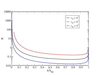
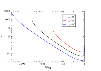
Figure 1: Numerical results for $\bar{n}(x)$ vs the ratio $x/x_{\scriptscriptstyle\rm M}$, computed from the Boltzmann equation (2.31) for three cases $x_{\scriptscriptstyle\rm M}=10^{2}$ (red, top), $10^{3}$ (black, middle), and $10^{4}$ (blue, bottom). The left frame uses a linear scale for the $x$-axis, whereas the right frame uses logarithmic scales on both axes. The IR regulator has been set to $\kappa=1$.

Numerical solutions for the choice of $\kappa=1$ and $x_{\scriptscriptstyle\rm M}=10^{2},\,10^{3}$ and $10^{4}$ are presented in fig. 1. We present the solutions in plots against $x/x_{\scriptscriptstyle\rm M}$ as defined in (2.27). The overall shape of the curves evidently does not depend on $x_{\scriptscriptstyle\rm M}$. Starting at $x=x_{\scriptscriptstyle\rm M}$ the solution at first drops quickly; this part of the curves can better be seen in the left frame, which uses a linear scale for the $x$-axis. Initially this decline simply reflects the $(x_{\scriptscriptstyle\rm M}-x)^{-3/2}$ dependence of the integration kernel applied to the $\delta$-function at $x=x_{\scriptscriptstyle\rm M}$. However, this contribution becomes sub-leading already at $x\leq x_{\scriptscriptstyle\rm M}-3$, where iterated emission processes become important, and lead to a flattening of the spectrum. Somewhat counter-intuitively, the $\sqrt{2/x}$ term in the denominator of the Boltzmann equation (2.31) is quite important even in the large$-x$ region; without this term, the spectrum would reach a (much lower) minimum at $x\>\raisebox{-2.15277pt}{$\stackrel{{\scriptstyle\textstyle<}}{{\sim}}$}\>x_{\scriptscriptstyle\rm M}/2$. Instead, via the cumulative effect of the small variation due to the square root, the curves in Fig. 1 reach their minimum at $x_{-}\simeq 0.78x_{\scriptscriptstyle\rm M}$; to very good approximation the $x$-value where the minimum is reached is proportional to $x_{\scriptscriptstyle\rm M}$, i.e. the minimum is reached at a fixed ratio $x/x_{\scriptscriptstyle\rm M}$.

Figure 1 further shows that, as expected, the spectrum rises again towards smaller values of $x$. This part of the spectrum is more readily studied using a logarithmic scale for the $x$-axis (right frame). We see that for $10\leq x\leq x_{-}/2$ the spectrum can be described by a falling power of $x$. The numerical value of this power is close to $-3/2$. This reflects the $E_{\scriptscriptstyle\rm d}^{-3/2}$ dependence of the LPM splitting rate, see eq.(2.15), and agrees with [22, 62, 58]. Finally, for $x\leq 10$ the spectrum bends upwards, as the $x^{\prime}$-independent denominator in eq.(2.31) develops a strong $x$-dependence.

These features of the spectrum mentioned so far are relatively independent of $x_{\scriptscriptstyle\rm M}$. However, the absolute value of the spectrum at fixed $x$, or fixed ratio $x/x_{\scriptscriptstyle\rm M}$, clearly does depend on $x_{\scriptscriptstyle\rm M}$. In fact, to a good approximation, the solution $\bar{n}$ at fixed $x/x_{\scriptscriptstyle\rm M}$ scales like $1/\sqrt{x_{\scriptscriptstyle\rm M}}$, unless $x\leq 10$ where the low$-x$ rise described above becomes pronounced. This can be understood from the observation that the thermalization time of eq.(2.17) scales like $\sqrt{M}\propto\sqrt{x_{\scriptscriptstyle\rm M}}$: the total number of non-thermal particles should be proportional to the thermalization time; since the spectrum is spread out over a wider energy range when $M$ increases, the differential spectrum at fixed $x/x_{\scriptscriptstyle\rm M}$ should scale like $t_{\scriptscriptstyle\rm therm}/M\propto 1/\sqrt{x_{\scriptscriptstyle\rm M}}$. This also explains why the spectrum scales linearly in $x_{\scriptscriptstyle\rm M}$ at fixed small $x$: the decreasing normalization at fixed $x/x_{\scriptscriptstyle\rm M}$ $\propto 1/\sqrt{x_{\scriptscriptstyle\rm M}}$ is over-compensated by the $(x/x_{\scriptscriptstyle\rm M})^{-3/2}$ behavior at fixed $x$ (well below the location of the minimum).

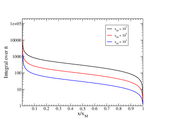
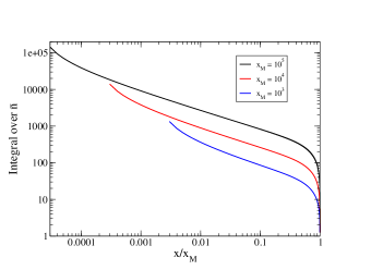
Figure 2: Numerical results for $\int_{x}^{x_{\scriptscriptstyle\rm M}}\bar{n}(x^{\prime})\,dx^{\prime}$ vs the ratio $x/x_{\scriptscriptstyle\rm M}$, computed from the Boltzmann equation (2.31) for three cases $x_{\scriptscriptstyle\rm M}=10^{5}$ (black, top), $10^{4}$ (red, middle), and $10^{3}$ (blue, bottom). The left frame uses a linear scale for the $x$-axis, whereas the right frame uses logarithmic scales on both axes. The IR regulator has been set to $\kappa=1$.

In some applications, the total number of energetic, non-thermal particles of energies above $E$ may be important. In fig. 2 we therefore show results for the integral $\int_{x}^{x_{\scriptscriptstyle\rm M}}\bar{n}(x^{\prime})\,dx^{\prime}$, again as function of the ratio $x/x_{\scriptscriptstyle\rm M}$, for three values of $x_{\scriptscriptstyle\rm M}$ now extending to $x_{\scriptscriptstyle\rm M}=10^{5}$. We see that the integral quickly increases when $x$ is reduced from $x_{\scriptscriptstyle\rm M}$; this reflects the spike at large $x$ seen in Fig. 1. This is followed, in the vicinity of the broad minimum of $\bar{n}$, by a rather flat plateau where the integral increases relatively slowly (note, however, the logarithmic scale of the $y$-axis). At smaller $x$ the integral increases $\propto(x/x_{\scriptscriptstyle\rm M})^{-1/2}$. This power-law behavior, which is again better seen with a logarithmic $x$-axis (right frame), evidently reflects the $(x/x_{\scriptscriptstyle\rm M})^{-3/2}$ behavior of $\bar{n}$ noted above. The upturn at $x\leq 10$ is again due to the $x$-dependence of the factor in front of the integral in eq.(2.31).

As expected from the above discussion of the thermalization time, the value of the integral at fixed $x/x_{\scriptscriptstyle\rm M}$ increases $\propto\sqrt{x_{\scriptscriptstyle\rm M}}$ as long as $x\>\raisebox{-2.15277pt}{$\stackrel{{\scriptstyle\textstyle>}}{{\sim}}$}\>10$. Together with the $1/\sqrt{x}$ dependence of the integral at fixed $x_{\scriptscriptstyle\rm M}$ this implies that the total number of non-thermal particles, i.e. the integral starting at $x=3$ (or a similar fixed, low value), increases essentially linearly with $x_{\scriptscriptstyle\rm M}$. This is very reasonable: at the end of the particle cascade, the total number of particles in the cascade should be proportional to the initially injected energy, i.e. to $x_{\scriptscriptstyle\rm M}$.

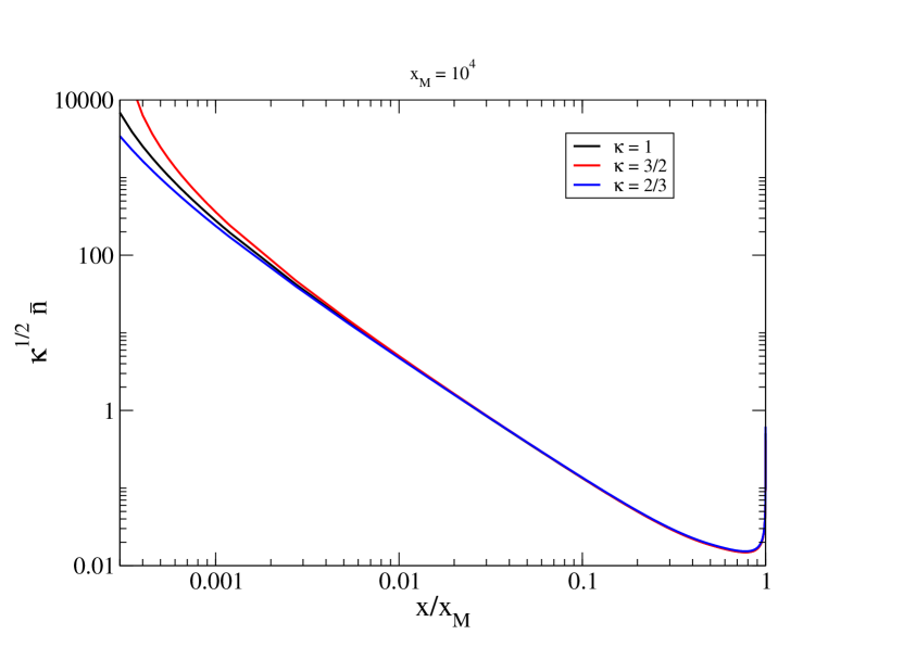
Figure 3: Numerical results for $\sqrt{\kappa}\cdot\bar{n}(x)$ vs the ratio $x/x_{\scriptscriptstyle\rm M}$, computed from the Boltzmann equation (2.31), with $x=10^{4}$ and three different values of the IR regulator $\kappa$: $1$ (black), $3/2$ and $2/3$ (blue). $\bar{n}$ has been multiplied with $\sqrt{\kappa}$ in order to remove the $\kappa$-dependence of the normalization factor $\widetilde{N}_{\scriptscriptstyle\rm M}$ defined in eq.(2.24). The three curves essentially lie on top of each other for $x/x_{\scriptscriptstyle\rm M}\>\raisebox{-2.15277pt}{$\stackrel{{\scriptstyle\textstyle>}}{{\sim}}$}\>0.01$, i.e. $x\>\raisebox{-2.15277pt}{$\stackrel{{\scriptstyle\textstyle>}}{{\sim}}$}\>100$.

As stated earlier, the results presented so far have all been obtained with our default choice for the IR regulator $\kappa=1$. We can now address the effects of the choice of $\kappa$. It is reasonable to expect the physical solution to be fairly independent of the specific choice of thermal cutoff. The physical (non-normalized) density of particles in the thermal spectrum is proportional to $\widetilde{N}_{\scriptscriptstyle\rm M}\cdot\bar{n}$, and so using (2.24) proportional to $\bar{n}/\Gamma^{\rm split}_{\scriptscriptstyle\rm LPM}$. Furthermore, we know from (2.22) that $\Gamma^{\rm split}_{\scriptscriptstyle\rm LPM}\propto 1/\sqrt{\kappa}$ for $\sqrt{x_{\scriptscriptstyle\rm M}}\gg 1$. Hence we can expect the combination $\sqrt{\kappa}\bar{n}$ to be $\kappa$-independent.

In fig. 3 we present results for $\sqrt{\kappa}\cdot\bar{n}$, with a fixed $x_{\scriptscriptstyle\rm M}=10^{4}$ as an example, using three different values of $\kappa$. The agreement among different solutions imply that the physical density computed from our formalism is indeed almost independent of $\kappa$, except for the region $x\>\raisebox{-2.15277pt}{$\stackrel{{\scriptstyle\textstyle<}}{{\sim}}$}\>10$ where an increase of $\kappa$ begins to significantly increase the time needed to complete the thermalization; recall that we do not admit emission of daughter particles with energy below $\kappa T$. We checked numerically that the results indeed depend on $\kappa$ significantly only for $x\>\raisebox{-2.15277pt}{$\stackrel{{\scriptstyle\textstyle<}}{{\sim}}$}\>10$, independent of the value of $x_{\scriptscriptstyle\rm M}$. This is also well expected, as it is an effect of the saturation exclusively due to the presence of the thermal bath of temperature $T$.

3.2 Analytical Parametrization

In this subsection we wish to find an analytical approximation to the exact numerical solution. A simple fitted function would obviously be much easier to compute; this can be very advantageous in numerical applications, e.g. when many values of $x_{\scriptscriptstyle\rm M}$ need to be investigated. Note that $x_{\scriptscriptstyle\rm M}=M/(2T)$ in general changes during the epoch of energy injection, since $T$ decreases as $\propto t^{-1/2}\ (t^{-1/4})$ if $\rho_{\scriptscriptstyle\rm M}\ll\rho_{\scriptscriptstyle\rm R}\ (\rho_{\scriptscriptstyle\rm M}\gg\rho_{\scriptscriptstyle\rm R})$.

Let us first exploit our understanding of the properties of the solution to narrow down candidates for the fitting function. Obviously an approximation will be more accessible if it only depends on the ratio $x/x_{\scriptscriptstyle\rm M}$, rather than on $x$ and $x_{\scriptscriptstyle\rm M}$ separately. In the previous subsection we saw that $\bar{n}$ indeed has a rather similar shape for different values of $x_{\scriptscriptstyle\rm M}$; we also saw that the value of $\bar{n}$ at fixed $x/x_{\scriptscriptstyle\rm M}$ scales basically like $1/\sqrt{x_{\scriptscriptstyle\rm M}}$ if $x\gg 1$.

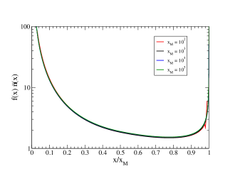
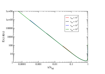
Figure 4: Numerical results for $f(x)\cdot[\bar{n}(x)-\delta(x-x_{\scriptscriptstyle\rm M})]$ vs the ratio $x/x_{\scriptscriptstyle\rm M}$. $\bar{n}$ has been computed from the Boltzmann equation (2.31) for four values of $x_{\scriptscriptstyle\rm M}$, with IR regulator $\kappa=1$. The function $f(x)$ as defined in eq.(3.2) has been chosen such that the four curves almost fall on top of each other. The left (right) frame uses a linear (logarithmic) scale for the $x$-axis.

As can be seen in Fig. 4, to very good approximation a function that only depends on the ratio $x/x_{\scriptscriptstyle\rm M}$ results if the solution of the Boltzmann equation (2.31) (without the $\delta$-function at $x=x_{\scriptscriptstyle\rm M}$, which is always normalized to unity) is multiplied with the function

$$f(x,x_{\scriptscriptstyle\rm M})=\sqrt{x_{\scriptscriptstyle\rm M}}\frac{\left(1-\sqrt{2/x}\right)^{5/4}}{1-2/\sqrt{x_{\scriptscriptstyle\rm M}}}\,.$$ (3.2)

The factor of $\sqrt{x_{\scriptscriptstyle\rm M}}$ has already been remarked upon. The denominator in (3.2) removes the $x_{\scriptscriptstyle\rm M}$ dependence that results from $\Gamma^{\rm split}_{\scriptscriptstyle\rm LPM}$. The numerator compensates the prefactor $1/(1-\sqrt{2/x})$ of the integral in the Boltzmann equation (2.31), where the power $5/4$ has been adjusted to make the curves in Fig. 4 approximately coincide.

Note that another piece of the solution, namely the delta function at $x=x_{\scriptscriptstyle\rm M}$, is already available. Moreover, the inclusion of the delta function will further imply that in the immediate neighborhood of $x_{\scriptscriptstyle\rm M}$ one should have

$$\left.\bar{n}(x)\right|_{x\simeq x_{\scriptscriptstyle\rm M}}\simeq\frac{1}{2}\int_{x+1}^{x_{\scriptscriptstyle\rm M}}\delta(x^{\prime}-x_{\scriptscriptstyle\rm M})(x^{\prime}-x)^{-3/2}dx^{\prime}=\frac{1}{2}(x_{\scriptscriptstyle\rm M}-x)^{-3/2}\,.$$ (3.3)

However, this merely includes the contribution of a single splitting starting from $x=x_{\scriptscriptstyle\rm M}$. The numerical analysis shows that this becomes inadequate already at $x_{\scriptscriptstyle\rm M}-x\simeq 3$; recall that for $x_{\scriptscriptstyle\rm M}-x\>\raisebox{-2.15277pt}{$\stackrel{{\scriptstyle\textstyle<}}{{\sim}}$}\>3$ our solution is in any case not reliable, due to the dependence on the hard IR cutoff $\kappa$. Nevertheless the numerical results clearly show that the spectrum initially falls off with decreasing $x$. We parameterize this through a negative power in $(x_{\scriptscriptstyle\rm M}-x)$. On the other hand, for $1\ll x\ll x_{\scriptscriptstyle\rm M}$ we found that the spectrum basically scales as $x^{-3/2}$; fig. 4 shows that after multiplying $\bar{n}(x)$ with the function $f(x)$ this scaling holds for all $x\ll x_{\scriptscriptstyle\rm M}$.

This suggests the ansatz

$$f(x,x_{\scriptscriptstyle\rm M})\cdot\left[\bar{n}(x,x_{\scriptscriptstyle\rm M})-\delta(x-x_{\scriptscriptstyle\rm M})\right]=a\left(\frac{x}{x_{\scriptscriptstyle\rm M}}\right)^{-3/2}\left(1-\frac{x}{x_{\scriptscriptstyle\rm M}}\right)^{-b}+c\,,$$ (3.4)

where the constant $c$ has been introduced in order to improve the description of the numerical result near the minimum. Our final fitting function for the spectrum of non-thermal particles is thus:

$$\bar{n}(x,x_{\scriptscriptstyle\rm M})=\delta(x-x_{\scriptscriptstyle\rm M})+\frac{\left[a\left(x/x_{\scriptscriptstyle\rm M}\right)^{-3/2}\left(1-x/x_{\scriptscriptstyle\rm M}\right)^{-b}+c\right]\left(1-2/\sqrt{x_{\scriptscriptstyle\rm M}}\right)}{\sqrt{x_{\scriptscriptstyle\rm M}}\left(1-\sqrt{2/x}\right)^{5/4}}\,.$$ (3.5)

As an example, in the case of $x_{\scriptscriptstyle\rm M}=10^{5}$, the following choice of parameters leads to an average deviation between numerical result and fit of about $2\%$:

$$a=0.39,\ b=0.48,\ c=0.37\,.$$ (3.6)

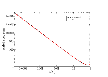
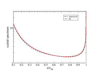
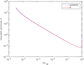
Figure 5: Fit (solid, red) of the form (3.4) and (3.5) compared to the numerical result (dashed, black) for the scaled spectrum $f(x,x_{\scriptscriptstyle\rm M})\bar{n}(x,x_{\scriptscriptstyle\rm M})$ (top left and top right) and non-scaled spectrum $\bar{n}(x,x_{\scriptscriptstyle\rm M})$ (bottom). The numerical results are for IR regulator $\kappa=1$ and $x_{\scriptscriptstyle\rm M}=10^{5}$, however the results shown in the top figures practically only depend on the ratio $x/x_{\scriptscriptstyle\rm M}$ as long as $x\geq 1$.

In fact, for values of $0.35\leq a\,,b\,,c\leq 0.45$ the numerical results can be reproduced by a solution of the form (3.4) within $3\%$ average error, across four orders of magnitude. In Fig. 5 we compare the fit function with the exact numerical result for the rescaled spectrum $f\cdot\bar{n}$; the latter has been computed for $x_{\scriptscriptstyle\rm M}=10^{5}$, but we saw above that the rescaled spectrum practically only depends on the ratio $x/x_{\scriptscriptstyle\rm M}$ as long as $x\geq 1$. Similarly, the bottom frame in Fig. 5 shows the agreement between the numerical results and fits of form (3.5) to the numerical solution. We see that the fit not only describes the overall behavior well (left frame), but also the spike at $x\simeq x_{\scriptscriptstyle\rm M}$ as well as the minimum at $x\simeq 0.78x_{\scriptscriptstyle\rm M}$ (right frame). Recall that these results hold for IR cutoff $\kappa=1$, but we saw at the end of the previous Subsection that taking a different ${\cal O}(1)$ value for $\kappa$ only affects the solution at $x\>\raisebox{-2.15277pt}{$\stackrel{{\scriptstyle\textstyle<}}{{\sim}}$}\>10\kappa$ and $x_{\scriptscriptstyle\rm M}-x\>\raisebox{-2.15277pt}{$\stackrel{{\scriptstyle\textstyle<}}{{\sim}}$}\>10\kappa$.

3.3 Application: Production of (Meta-)stable Relics

To conclude, we will briefly review an example for the applications of a spectrum of type (3.5) in calculating quantities of interest in cosmology. To that end, we will adopt the notations and results from [12] along with results from [22] for comparison. For an era where the decay products dominate the thermal bath, authors in [12] use the number density of primary decay products of energy $M/2$, given by

$$n_{h}\left({T}\right)\sim\rho/M\sim 0.3\,g_{*}T^{4}/M.$$ (3.7)

Partly based on dimensional analysis, the authors in [22] instead suggested an analytical solution of the form

$$\tilde{n}_{\scriptscriptstyle\rm An}(p)=\frac{n_{\scriptscriptstyle\rm M}\Gamma_{\scriptscriptstyle\rm M}M}{\sqrt{\tilde{g}_{*}}\alpha^{2}T^{3/2}}p^{-3/2}\,,$$ (3.8)

for the spectrum of thermalizing decay products. In this setup, one may further identify $\Gamma_{\scriptscriptstyle\rm M}\cdot n_{\scriptscriptstyle\rm M}\cdot M\cdot t_{\scriptscriptstyle\rm H}\approx\rho_{\scriptscriptstyle\rm R}\left({T}\right)$ to fix $\tilde{N}_{\scriptscriptstyle\rm M}$ in (2.25), and so the normalization of the solution $\tilde{n}\left({p}\right)$ in (2.30) as well as (3.8).

In order to outline the consequences of the presence and the form of a spectrum of energetic particles as in (3.5) and (3.8), we will revisit the production of heavy (meta-)stable particles prior to reheating in a matter-dominated universe, and point out further possible consequences for cosmology. Let us assume we are interested in the production of a heavy species $\chi$ with a mass $m_{\scriptscriptstyle\rm\chi}\gg T_{\scriptscriptstyle\rm RH}$. The high mass of species $\chi$ implies that, in addition to processes among soft particles in the thermal bath, $\chi$ production via interactions of the hard thermalizing decay products with the soft (hard-soft processes), or other hard (hard-hard processes) particles can become important.

The authors in [12] have used $2\rightarrow 3$ splitting processes with a massless gauge boson as the t-channel propagator to calculate a slow-down(thermalization) rate of

$$\Gamma_{\rm slow}\simeq 3\alpha^{3}T\left(\frac{g_{*}}{200}\right)^{1/3}.$$ (3.9)

To regulate the process rate, the IR cutoff has been chosen as $n_{\scriptscriptstyle\rm R}^{1/3}\left({T}\right)$, with $n_{\scriptscriptstyle\rm R}$ given by (2.2b), corresponding to the average spacing of particles in the thermal bath. As such, the hallmark energy-dependence of the LPM effect (see (2.17)) is absent from (3.9). The primary decay products (3.7) are assumed to constitute the out-of-equilibrium particles contributing to the $\chi$ production, so that the hard-soft production rate takes the form

$$\Gamma^{\scriptscriptstyle\rm hs}_{\chi}\sim 0.2\,\left(\frac{\alpha^{2}_{\chi}}{TM}+\frac{\alpha\alpha_{\chi}^{2}}{m_{\chi}^{2}}\right)T^{3}.$$ (3.10)

The coupling of $\chi$ to a single species of the thermal bath is parameterized via $\alpha_{\scriptscriptstyle\rm\chi}$. As can be seen from the denominators of (3.10), the hard-soft cross section for the number density (3.7) of primary decay particles of energy $M/2$ will either suffer from large energy suppression or will have to resort to radiating away the extra energy at the cost of an extra power of $\alpha$, resulting in a number density for $\chi$’s reading

$$n_{\chi}^{\scriptscriptstyle\rm hs}(T)\sim n_{h}\cdot\frac{\Gamma^{\rm hs}_{\chi}}{\Gamma_{\scriptscriptstyle\rm slow}}\sim 4\left(\frac{g_{*}}{200}\right)^{2/3}\frac{\alpha_{\chi}^{2}}{\alpha^{2}}\left(\frac{T^{5}}{\alpha M^{2}}+\frac{T^{6}}{Mm_{\chi}^{2}}\right).$$ (3.11)

The splitting cascade underlying the spectra (3.5) and (3.8) provides a larger number density of particles of lower energy, simultaneously increasing initial state density and $\Gamma_{\chi}^{\scriptscriptstyle\rm hs}$, so that now

$$\Gamma^{\scriptscriptstyle\rm hs}_{\chi}\left({p}\right)\sim 0.2\frac{\alpha^{2}_{\chi}}{pT}T^{3}\mathcal{H}\left({pT-p_{\scriptscriptstyle\rm thr}T}\right)$$ (3.12)

where $\mathcal{H}$ is the Heaviside step function, and with the kinematic threshold $p_{\scriptscriptstyle\rm thr}=\beta m_{\scriptscriptstyle\rm\chi}^{2}/T$, and $\beta$ a parameter of $\mathcal{O}\left({1}\right)$ setting the kinematic production threshold. The number density of $\chi$’s produced during a Hubble time $t_{\scriptscriptstyle\rm H}$ can be written as

$$n_{\scriptscriptstyle\rm\chi}^{\scriptscriptstyle\rm hs}\left({T}\right) = t_{\scriptscriptstyle\rm H}\int_{p_{\scriptscriptstyle\rm thr}}^{M/2}\Gamma^{\scriptscriptstyle\rm hs}_{\scriptscriptstyle\rm\chi}\left({p}\right)dn\left({p}\right)=t_{\scriptscriptstyle\rm H}\int_{p_{\scriptscriptstyle\rm thr}}^{M/2}\Gamma_{\scriptscriptstyle\rm\chi}^{\scriptscriptstyle\rm hs}\left({p}\right)\tilde{n}\left({p}\right)dp.$$ (3.13)

A comparison with (3.11) shows, that the yield in (3.13) can be parametrically larger.

A finer comparison is between the hard-soft yield resulting from the two numeric (3.5) and analytic (3.8) solutions for a certain $x_{\scriptscriptstyle\rm M}$. To that end, let us first rewrite the two spectra as

$$\left.\begin{aligned} &\tilde{n}_{\scriptscriptstyle\rm Num}(p)&\\ &\tilde{n}_{\scriptscriptstyle\rm An}(p)&\end{aligned}\right\}=\left({\frac{\tilde{N}_{\scriptscriptstyle\rm M}}{T}}\right)\times\left\{\begin{aligned} &\bar{n}_{\scriptscriptstyle\rm Num}\left({x}\right)&\\ &\bar{n}_{\scriptscriptstyle\rm An}\left({x}\right)=\frac{2}{\sqrt{x_{\scriptscriptstyle\rm M}}}\left({x/x_{\scriptscriptstyle\rm M}}\right)^{-3/2}&\end{aligned}\right.,$$ (3.14)

where $\bar{n}_{\scriptscriptstyle\rm Num}\left({x}\right)$ is given in (3.5), and we have used (2.28) to relate $\tilde{n}\left({p}\right)$ and $\tilde{n}\left({x}\right)$. Motivated by the form of (3.13) and the relative sensitivity to near threshold energies $p_{\scriptscriptstyle\rm thr}$ for a heavy $\chi$, we may directly compare the two spectra using the integrated weighted spectrum

$$n_{\scriptscriptstyle\rm\chi}^{\scriptscriptstyle\rm hs}\left({T}\right)\propto\frac{t_{\scriptscriptstyle\rm H}n_{\scriptscriptstyle\rm R}\alpha_{\scriptscriptstyle\rm\chi}^{2}}{T}\int_{p}^{M/2}\frac{\tilde{n}\left({p^{\prime}}\right)}{p^{\prime}}\,dp^{\prime}=\left({\frac{t_{\scriptscriptstyle\rm H}n_{\scriptscriptstyle\rm R}\alpha_{\scriptscriptstyle\rm\chi}^{2}\tilde{N}_{\scriptscriptstyle\rm M}}{T^{2}}}\right)\int_{x}^{x_{\scriptscriptstyle\rm M}}\frac{\bar{n}\left({x^{\prime}}\right)}{x^{\prime}}\,dx^{\prime}.$$ (3.15)

Figure 6(top-left) shows the integrated weighted spectra from the two forms in (3.14), and the corresponding relative error of an analytical approximation compared to a full numerical solution for the two cases $x_{\scriptscriptstyle\rm M}=10^{3}$ and $10^{5}$. The figure on the right further shows that an error of $\mathcal{O}(1)$ is expected by using the monotonic form of the particle spectrum $\tilde{n}_{\scriptscriptstyle\rm An}$.

In scenarios where $m_{\scriptscriptstyle\rm\chi}$ is large enough so that at the end of reheating $p_{\scriptscriptstyle\rm thr}\gg M$, the hard-soft channel of production might be either kinematically forbidden, or highly suppressed due to subsequent entropy production via the matter decay process. In such cases, interactions among the less abundant hard states could contribute to the production of $\chi$’s. Once again we will begin by presenting the hard-hard yield using the initial number density of particles of energy $M/2$ in the setup from [12]. The transient nature of out-of-equilibrium states implies that one should use the instantaneous number density. Specializing again to a case where the decays dominate the thermal bath of a Hubble era of temperature $T$, one can write

$$n_{\scriptscriptstyle\rm h}^{\scriptscriptstyle\rm inst}\left({T}\right)\sim Hg_{*}T^{4}/3\Gamma_{\scriptscriptstyle\rm slow}M,$$ (3.16)

which subsequently leads to a $\chi$ number density [12]

$$n_{\chi}^{\rm hh}(T)\sim n_{\scriptscriptstyle\rm h}^{\scriptscriptstyle\rm inst}\Gamma_{\scriptscriptstyle\rm\chi}^{\scriptscriptstyle\rm hh}t_{\scriptscriptstyle\rm H}\quad\texttt{with, }\Gamma_{\scriptscriptstyle\rm\chi}^{\scriptscriptstyle\rm hh}=\sigma_{\scriptscriptstyle\rm\chi}^{\scriptscriptstyle\rm hh}n_{\scriptscriptstyle\rm h}^{\scriptscriptstyle\rm inst}=\left(\frac{\alpha_{\chi}^{2}}{M^{2}}+\frac{\alpha\alpha_{\chi}^{2}}{m_{\chi}^{2}}\right)n_{\scriptscriptstyle\rm h}^{\scriptscriptstyle\rm inst}.$$ (3.17)

Note that the target density in (3.17) reflects the transient nature of the hard-hard process, and that the second term in the cross section would once more radiatively return the center of mass energy to the production threshold of $\chi$ particles.

On the other hand, in the presence of continuous spectrum of states (3.5) and (3.8), the hard-hard production can be estimated as

$$n_{\chi}^{\rm hh}(T)\sim\int_{T}^{M/2}\int_{T}^{M/2}\tilde{n}\left({p}\right)\tilde{n}\left({p^{\prime}}\right)\sigma_{\scriptscriptstyle\rm\chi}^{\scriptscriptstyle\rm hh}\left({p,p^{\prime}}\right)dp\,dp^{\prime}\,t_{\scriptscriptstyle\rm H},\quad\sigma_{\scriptscriptstyle\rm\chi}^{\scriptscriptstyle\rm hh}\left({p,p^{\prime}}\right)=\frac{\alpha_{\chi}^{2}}{pp^{\prime}}\,\mathcal{H}\left({pp^{\prime}-\beta m_{\scriptscriptstyle\rm\chi}^{2}}\right).$$ (3.18)

The integral is then calculated numerically for a spectrum as in (3.5). In the case $m_{\scriptscriptstyle\rm\chi}$ is sufficiently smaller than $M$, however, we may use the approximation $\tilde{n}(p\ll M)\propto p^{-3/2}$ to put the solution in the form of (3.17) where now

$$n_{\scriptscriptstyle\rm h}^{\scriptscriptstyle\rm inst}\left({T}\right)\approx Hg_{*}T^{4}/\Gamma_{\scriptscriptstyle\rm Th}\left({m_{\scriptscriptstyle\rm\chi}}\right)m_{\scriptscriptstyle\rm\chi},\quad\texttt{and}\quad\sigma_{\scriptscriptstyle\rm\chi}^{\scriptscriptstyle\rm hh}=\alpha_{\scriptscriptstyle\rm\chi}^{2}/m_{\scriptscriptstyle\rm\chi}^{2},$$ (3.19)

resulting in a sizable enhancement as compared to (3.17).

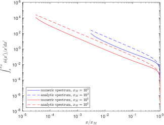
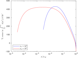
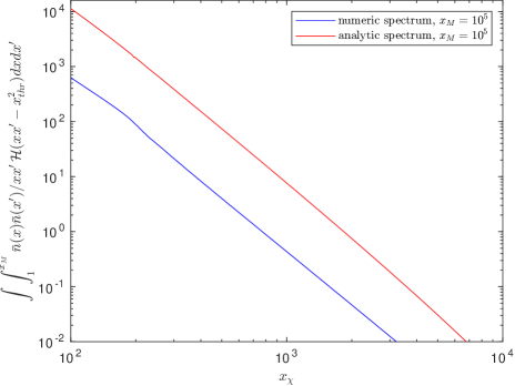
Figure 6: (Top-left) Scaled integrated weighted spectrum (3.15), resulting from the the two spectra from (3.14) versus $x/x_{\scriptscriptstyle\rm M}$ for two cases with $x_{\scriptscriptstyle\rm M}=10^{3}$(blue), and $10^{5}$(red). (Top-right) The relative error in (3.15) stemming from a monotonic spectrum. (Bottom) Scaled hard-hard yield from (3.20), resulting from the two spectra in (3.14) and the case of $x_{\scriptscriptstyle\rm M}=10^{5}$.

One can also employ equation (3.18) to find how large an effect differentiates the two spectra in (3.14). This is shown in figure 6(bottom), where we plot the resulting number density for a range of $\chi$ masses between $T_{\scriptscriptstyle\rm RH}\cdot 10^{2}$ and $M/2$, and have again factored out the prefactors in (3.18) as

$$n_{\chi}^{\rm hh}(T)\sim\left({t_{\scriptscriptstyle\rm H}\,\alpha_{\scriptscriptstyle\rm\chi}^{2}\,\tilde{N}_{\scriptscriptstyle\rm M}^{2}\,/\,T^{2}}\right)\iint^{x_{\scriptscriptstyle\rm M}}_{1}\frac{\bar{n}\left({x}\right)\bar{n}\left({x^{\prime}}\right)}{x\,x^{\prime}}\,\mathcal{H}\left({xx^{\prime}-x_{\scriptscriptstyle\rm thr}^{2}}\right)dx\,dx^{\prime},$$ (3.20)

to better capture the effect of the two spectra. In (3.20), we have once more introduced the cutoff as $x_{\scriptscriptstyle\rm thr}^{2}=\beta x_{\scriptscriptstyle\rm\chi}^{2}=\beta m_{\scriptscriptstyle\rm\chi}^{2}/T^{2}$ for the kinetically allowed region. Figure 6(bottom) shows that while the combination of different parts of the spectrum in (3.20) flattens the resulting spectrum as compared to (3.5), an order of magnitude effect is observed, similar to the case of hard-soft production.

Finally, we can use the $\Omega-$ parameter to translate the number densities $n_{\scriptscriptstyle\rm\chi}^{\scriptscriptstyle\rm hh}$ and $n_{\scriptscriptstyle\rm\chi}^{\scriptscriptstyle\rm hs}$ into energy density fraction today $\left({\Omega h^{2}}\right)_{\scriptscriptstyle\rm\chi}$, to make easier contact with the observed quantities. The contribution of $n_{\scriptscriptstyle\rm\chi}\left({T}\right)$, from an era of temperature $T$, to the omega parameter today can be written as

$$\left({\Omega h^{2}}\right)_{\scriptscriptstyle\rm\chi}\left({T}\right)\sim\frac{n_{\scriptscriptstyle\rm\chi}\left({T}\right)}{s\left({T}\right)}\frac{T_{\scriptscriptstyle\rm RH}^{5}}{T^{5}}\frac{m_{\scriptscriptstyle\rm\chi}}{T_{\scriptscriptstyle\rm 0}}\left({\Omega h^{2}}\right)_{\scriptscriptstyle\rm R},$$ (3.21)

with $T_{\scriptscriptstyle\rm 0}=0.24$ meV denoting the radiation temperature today, and $\left({\Omega h^{2}}\right)_{\scriptscriptstyle\rm R}=4.3\cdot 10^{-5}$.

The resulting temperature dependence of the hard-soft and hard-hard diluted yields imply that the former is dominated at the lowest available temperature $T_{\scriptscriptstyle\rm thr}=\max(\beta m_{\scriptscriptstyle\rm\chi}^{2}/M,T_{\scriptscriptstyle\rm RH})$, while the latter will be set by the maximum temperature of the thermal bath $T_{\scriptscriptstyle\rm max}$, given by

$$T_{\rm max}\sim T_{\scriptscriptstyle\rm RH}\left(\alpha^{3}\left(\frac{g_{*}}{3}\right)^{1/3}{M_{\rm Pl}\over M^{1/3}T_{\scriptscriptstyle\rm RH}^{2/3}}\right)^{3/8}.$$ (3.22)

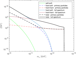
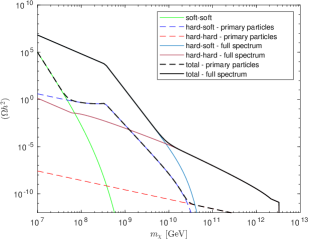
Figure 7: Energy density fraction parameter $\left({\Omega h^{2}}\right)_{\scriptscriptstyle\rm\chi}$ resulting from hard-soft(3.11, 3.13), hard-hard(3.17, 3.18), and thermal soft-soft (3.23) contributions with $\alpha_{\scriptscriptstyle\rm\chi}=0.01$, $\alpha=0.05$, $M=10^{13}$ GeV, and $T_{\scriptscriptstyle\rm RH}=10^{8}$ GeV ($T_{\scriptscriptstyle\rm RH}=10^{5}$ GeV) on the left(right). The dashed lines represent the resulting contribution from the primary number density of decay products[12](see Fig. a & b), while the solid lines correspond to production via the spectrum (3.5). The resulting hard-soft yield agrees with results in [22] within the errors discussed in figure 6 after accounting for the choice of production threshold energy, and the number of target species in the thermal bath. The knee-shaped effect at low $m_{\scriptscriptstyle\rm\chi}$ region in the case of $T_{\scriptscriptstyle\rm RH}=10^{5}$ GeV signifies of a change in $T_{\scriptscriptstyle\rm thr}$.

Figure 7 shows examples of the various contributions to $\left({\Omega h^{2}}\right)_{\scriptscriptstyle\rm\chi}$, given by using a number density of initial decay products as in [12] along those resulting from the corresponding processes using the full spectrum (3.5) for $x_{\scriptscriptstyle\rm M}=10^{5}$(left) and $x_{\scriptscriptstyle\rm M}=10^{8}$(right). The total abundance includes the sub-leading soft-soft production given by [28]

$$\left({\Omega h^{2}}\right)_{\scriptscriptstyle\rm\chi}^{\scriptscriptstyle\rm ss}\sim\left({200\over g_{*}}\right)^{3/2}\alpha_{\chi}^{2}{\left({2000T_{\rm RH}\over m_{\chi}}\right)}^{7}.$$ (3.23)

A sizable gain is evident in particle production by considering the full spectrum of the thermalization cascade. The dark coupling $\alpha_{\scriptscriptstyle\rm\chi}=0.01$ is chosen so as to reproduce the results in [12] for comparison, and thus lead to an overproduction of the species $\chi$. This could rather be understood as a suppression of the dark coupling $\alpha_{\scriptscriptstyle\rm\chi}$ required to reproduce a certain abundance for the species $\chi$. Note that in a general analysis, there could be other contributions from direct branching of the scalar field decays. If sizable, these channels will further increase the abundance or correspondingly lead to a further suppression of the dark coupling $\alpha_{\scriptscriptstyle\rm\chi}$. In figure 7 the hard-hard and hard-soft processes are shut down by an exponential suppression above $T_{\scriptscriptstyle\rm max}$ for simplicity. Slight deviation from a power low behavior in the intermediate regions of $m_{\scriptscriptstyle\rm\chi}$ for $\left({\Omega h^{2}}\right)^{\scriptscriptstyle\rm hh}_{\scriptscriptstyle\rm\chi}$ can be understood as resulting from contributions from a larger set of combinations of $p$ and $p^{\prime}$ in (3.18).

Finally, we will briefly discuss other potential consequences of considering the full spectrum of thermalizing states. We begin by pointing out that a sizable suppression of the dark coupling $\alpha_{\scriptscriptstyle\rm\chi}$ allows for an earlier kinetic decoupling of the species $\chi$ following production, as is the case for FIMP scenarios. As discussed in the literature, non-relativistic and kinetically decoupled DM perturbations grow linearly in the matter domination era, potentially affecting the matter spectrum[64, 65, 66]. While difficult to preserve in scenarios where the bulk of (relativistic) DM is generated thermally or directly via matter decays at the end of reheating era[64], viable scenarios might be realized using non-thermal production, e.g. via near-threshold production of DM from hard-hard scatterings. Note that after production at the threshold, the resulting abundance could then be rendered non-relativistic as a result of the Hubble expansion. Finally, a population of long lived $\chi$’s and its subsequent decay, can contribute to realizing cosmological processes, e.g. via formation of a later intermediate matter dominated era and/or late entropy production, generation of the baryon asymmetry(see e.g. [30] with superparticle decays), and dilution of preexisting abundances[67, 54, 17].

4 Summary and Conclusions

The high energetic decay products resulting from the decay of heavy out-of-equilibrium states are used for a plethora of applications in cosmology, including entropy production, the production of (meta-)stable relics (e.g. dark matter particles), baryogenesis, modifications of the expansion history and structure formation. While some of these applications rely solely on the presence of an extra contribution to the energy density content of the universe or the thermal bath, others depend critically on the energy distribution of the decay products prior to their complete thermalization.

In this paper we studied the energy spectrum of the chain of particles involved in the thermalization process. We have adopted the framework of thermalization via LPM suppressed $2\rightarrow 3$ splitting processes introduced in [22], paying special attention to the natural cutoffs and regulations of splitting rate divergences provided by the thermal plasma. These rely on the fact that particles exchange energies of order $T$ with the thermal bath relatively efficiently, via both emission and absorption processes as well as elastic scatterings. Therefore only the emission of particles with energy above $\kappa T$ needs to be included in the hard kernel of integral equations governing the momentum dispersion, with $\kappa$ acting as an IR cutoff parameter of order unity.

Since the thermalization time is typically much smaller than a Hubble time, the thermalization process can be treated at a fixed temperature $T$. This leads to a (quasi) steady state solution, described by the integral equation (2.21). After dividing out normalization factors, and introducing the dimensionless momentum (or energy) variable $x=p/T$, this led to the integral equation (2.31). This equation can be solved numerically by straightforward integration. After further normalization, the numerical solution to excellent approximation only depends on the ratio $x/x_{\scriptscriptstyle\rm M}=p/(2M)$, with $M$ denoting the mass of the decaying particle. This allowed us to find a simple, yet very accurate analytical fit function, given in eq.(3.5) which describes the numerical result to about $3\%$ accuracy.

This analytical approximation for the numerical solution to $\bar{n}(x)$ can easily be converted back to the original form using eqs.(2.25), (2.28) and (2.24). In particular, $\tilde{n}(p\ll M)$ is to very good approximation given by

$$\tilde{n}_{\scriptscriptstyle\rm Num}(p\ll M)=\frac{{\widetilde{N}}_{\scriptscriptstyle\rm M}\bar{n}(x\ll x_{\scriptscriptstyle\rm M})}{T}=0.39\frac{n_{\scriptscriptstyle\rm M}\Gamma_{\scriptscriptstyle\rm M}}{\sqrt{MT}\Gamma^{\rm split}_{\scriptscriptstyle\rm LPM}(M/2)}\cdot\left(1-\sqrt{2T/p}\right)^{-5/4}(p/M)^{-3/2}\,.$$ (4.1)

In camparison with (3.8), the leading power–law dependence of these two solutions, which dominates the spectrum for $p<M/4$, is the same. However, our solution contains an additional $p$-dependent factor. Moreover, our complete solution (3.5) contains another factor which generates a minimum at $p\simeq 0.39M$, followed by a spike as $p\rightarrow M/2$. As we’ve argued in section 2, the spectrum of non–thermal particles must be a rising function of $p$ near $p=M/2$. In contrast, the solution (3.8) suggested in [22] and further used in [23] shows a monotonous behavior in the entirety of the solution domain $M/2\leq p\leq T$. Moreover, the normalization of our solution (4.1) differs from that of (3.8) by the factor $a/\sqrt{\tilde{g}_{*}}$, which may be partly absorbed into the coupling parameter $\alpha$.

Both solutions lead to

$$\int_{0}^{M/2}\tilde{n}(p)pdp\propto\rho_{\scriptscriptstyle\rm M}\cdot\Gamma_{\scriptscriptstyle\rm M}\cdot t_{\scriptscriptstyle\rm therm}(M/2)$$ (4.2)

with $t_{\scriptscriptstyle\rm therm}$ given by (2.17). For $b=0.5$, close to the best-fit value of $0.48$, and ignoring the $x$-dependence in the denominator of eq.(3.5), the integral over our $p\tilde{n}(p)$ can be computed analytically. The numerical coefficient in eq.(4.2) is then $a\pi+c/2\simeq 1.4$, which is of order $1$ as expected. Note further that the contribution due to the $\delta$-function at $p=M/2$ to the integral in (4.2) is subdominant: it is $\propto 1/\Gamma_{\scriptscriptstyle\rm split}^{\rm LPM}=t_{\scriptscriptstyle\rm therm}\sqrt{T/M}$. Further, eq.(4.1) shows that a solution of the form (3.5) does indeed approach a growth $\propto M$ of the number density $dn/d\ln p$ at fixed $p$, as required by energy conservation.

Even though we believe our result to be more accurate and include more features than what is found in the literature, it clearly has some limitations. One issue is the hard IR cutoff, parameterized by the ${\cal O}(1)$ parameter $\kappa$. This isn’t particularly problematic, since we showed that the choice of $\kappa$ only affects the result for momenta which are either not much larger than $T$ (where the non-thermal spectrum gets swamped by the thermal contribution anyway), or where $M/2-p$ is of order $T$ (where the difference between $p$ and $M/2$ should be immaterial for all practical applications). More realistically, at the very low energies, there is an eventual smooth crossover into the regime where elastic processes in the thermal bath become competitive as an energy transfer mechanism. Once more, we have not considered the latter processes.

A much more serious approximation is the use of a single splitting kernel [68], given by eq.(2.15). While the leading $E_{\scriptscriptstyle\rm d}^{-3/2}$ dependence on the energy $E_{\scriptscriptstyle\rm d}$ of the softer daughter particle should indeed be universal, there will in general be additional terms depending on $E_{\scriptscriptstyle\rm d}/E_{\scriptscriptstyle\rm i}$, where $E_{\scriptscriptstyle\rm i}$ is the energy of the parent particle. These terms differ for different splitting reactions; for example, the emission of a gluon from a quark has a somewhat different kernel than that from another gluon. In order to treat them properly, one has to differentiate between different species of particles in the cascade, i.e. our single integral equation will have to be replaced by a set of coupled integral equations. However, the key parameter $E_{\scriptscriptstyle\rm d}$ has an expectation value of $\sqrt{TE_{\scriptscriptstyle\rm i}}$, while its most likely value is $\mathcal{O}(T)$. The large majority of splittings driving the thermalization process will therefore have $E_{\scriptscriptstyle\rm d}\ll E_{\scriptscriptstyle\rm i}$ and should be adequately described by our eq.(2.15).

As a last remark, we note that different species and interactions will in general appear in the solution with different overall factors. The formalism developed here can then be understood to hold for a suitable average over particle species. Getting these ${\cal O}(1)$ factors right is important only if all other parameters are known, including the mass and decay width, and the relevant decay modes of the parent particle, so that or results are sufficient to constrain these model parameters on a logarithmic scale. Considering the inevitable degeneracies in parameter-combinations (note, for example, that an ${\cal O}(1)$ change of the splitting rate $\Gamma^{\rm split}_{\scriptscriptstyle\rm LPM}$ can be compensated by a change in the decay width $\Gamma_{\scriptscriptstyle\rm M}$ of the parent particle, without invalidating (4.1)), our solution should suffice for most applications.

References

- [1] R. Allahverdi, R. Brandenberger, F. Y. Cyr-Racine and A. Mazumdar, “Reheating in Inflationary Cosmology: Theory and Applications,” Ann. Rev. Nucl. Part. Sci. 60 (2010), 27-51 doi:10.1146/annurev.nucl.012809.104511 [arXiv:1001.2600 [hep-th]].
- [2] G. Kane, K. Sinha and S. Watson, “Cosmological Moduli and the Post-Inflationary Universe: A Critical Review,” Int. J. Mod. Phys. D 24 (2015) no.08, 1530022 doi:10.1142/S0218271815300220 [arXiv:1502.07746 [hep-th]].
- [3] R. Allahverdi, M. A. Amin, A. Berlin, N. Bernal, C. T. Byrnes, M. Sten Delos, A. L. Erickcek, M. Escudero, D. G. Figueroa and K. Freese, et al. “The First Three Seconds: a Review of Possible Expansion Histories of the Early Universe,” doi:10.21105/astro.2006.16182 [arXiv:2006.16182 [astro-ph.CO]].
- [4] A. Di Marco and G. Pradisi, “Variable Inflaton Equation of State and Reheating,” [arXiv:2102.00326 [gr-qc]].
- [5] L. Visinelli, “(Non-)thermal production of WIMPs during kination,” Symmetry 10 (2018) no.11, 546 doi:10.3390/sym10110546 [arXiv:1710.11006 [astro-ph.CO]].
- [6] C. Maldonado and J. Unwin, “Establishing the Dark Matter Relic Density in an Era of Particle Decays,” JCAP 06 (2019), 037 doi:10.1088/1475-7516/2019/06/037 [arXiv:1902.10746 [hep-ph]].
- [7] L. Visinelli and P. Gondolo, “Axion cold dark matter in non-standard cosmologies,” Phys. Rev. D 81 (2010), 063508 doi:10.1103/PhysRevD.81.063508 [arXiv:0912.0015 [astro-ph.CO]].
- [8] M. A. G. Garcia, K. Kaneta, Y. Mambrini and K. A. Olive, “Inflaton Oscillations and Post-Inflationary Reheating,” [arXiv:2012.10756 [hep-ph]].
- [9] M. A. G. Garcia, K. Kaneta, Y. Mambrini and K. A. Olive, “Reheating and Post-inflationary Production of Dark Matter,” Phys. Rev. D 101 (2020) no.12, 123507 doi:10.1103/PhysRevD.101.123507 [arXiv:2004.08404 [hep-ph]].
- [10] J. T. Giblin, G. Kane, E. Nesbit, S. Watson and Y. Zhao, “Was the Universe Actually Radiation Dominated Prior to Nucleosynthesis?,” Phys. Rev. D 96 (2017) no.4, 043525 doi:10.1103/PhysRevD.96.043525 [arXiv:1706.08536 [hep-th]].
- [11] G. F. Giudice, E. W. Kolb and A. Riotto, “Largest temperature of the radiation era and its cosmological implications,” Phys. Rev. D 64 (2001), 023508 doi:10.1103/PhysRevD.64.023508 [arXiv:hep-ph/0005123 [hep-ph]].
- [12] R. Allahverdi and M. Drees, “Thermalization after inflation and production of massive stable particles,” Phys. Rev. D 66 (2002) 063513 doi:10.1103/PhysRevD.66.063513 [hep-ph/0205246]. R. Allahverdi and M. Drees, “Production of massive stable particles in inflaton decay,” Phys. Rev. Lett. 89 (2002), 091302 doi:10.1103/PhysRevLett.89.091302 [arXiv:hep-ph/0203118 [hep-ph]].
- [13] A. Berlin, D. Hooper and G. Krnjaic, “PeV-Scale Dark Matter as a Thermal Relic of a Decoupled Sector,” Phys. Lett. B 760 (2016), 106-111 doi:10.1016/j.physletb.2016.06.037 [arXiv:1602.08490 [hep-ph]].
- [14] A. Berlin, D. Hooper and G. Krnjaic, “Thermal Dark Matter From A Highly Decoupled Sector,” Phys. Rev. D 94 (2016) no.9, 095019 doi:10.1103/PhysRevD.94.095019 [arXiv:1609.02555 [hep-ph]].
- [15] S. Hamdan and J. Unwin, “Dark Matter Freeze-out During Matter Domination,” Mod. Phys. Lett. A 33 (2018) no.29, 1850181 doi:10.1142/S021773231850181X [arXiv:1710.03758 [hep-ph]].
- [16] P. Chanda, S. Hamdan and J. Unwin, “Reviving and Higgs Mediated Dark Matter Models in Matter Dominated Freeze-out,” JCAP 01 (2020), 034 doi:10.1088/1475-7516/2020/01/034 [arXiv:1911.02616 [hep-ph]].
- [17] R. T. Co, F. D’Eramo, L. J. Hall and D. Pappadopulo, “Freeze-In Dark Matter with Displaced Signatures at Colliders,” JCAP 1512 (2015) no.12, 024 doi:10.1088/1475-7516/2015/12/024 [arXiv:1506.07532 [hep-ph]].
- [18] M. A. G. Garcia and M. A. Amin, “Prethermalization production of dark matter,” Phys. Rev. D 98 (2018) no.10, 103504 doi:10.1103/PhysRevD.98.103504 [arXiv:1806.01865 [hep-ph]].
- [19] K. Ishiwata, “Axino Dark Matter in Moduli-induced Baryogenesis,” JHEP 09 (2014), 122 doi:10.1007/JHEP09(2014)122 [arXiv:1407.1827 [hep-ph]].
- [20] M. Dhuria, C. Hati and U. Sarkar, “Moduli induced cogenesis of baryon asymmetry and dark matter,” Phys. Lett. B 756 (2016), 376-383 doi:10.1016/j.physletb.2016.03.018 [arXiv:1508.04144 [hep-ph]].
- [21] J. Hasenkamp and J. Kersten, “Dark radiation from particle decay: cosmological constraints and opportunities,” JCAP 08 (2013), 024 doi:10.1088/1475-7516/2013/08/024 [arXiv:1212.4160 [hep-ph]].
- [22] K. Harigaya, M. Kawasaki, K. Mukaida and M. Yamada, “Dark Matter Production in Late Time Reheating,” Phys. Rev. D 89 (2014) no.8, 083532 doi:10.1103/PhysRevD.89.083532 [arXiv:1402.2846 [hep-ph]].
- [23] K. Harigaya, K. Mukaida and M. Yamada, “Dark Matter Production during the Thermalization Era,” arXiv:1901.11027 [hep-ph].
- [24] M. Drees and F. Hajkarim, “Neutralino Dark Matter in Scenarios with Early Matter Domination,” JHEP 1812 (2018) 042 doi:10.1007/JHEP12(2018)042 [arXiv:1808.05706 [hep-ph]].
- [25] M. Drees and F. Hajkarim, “Dark Matter Production in an Early Matter Dominated Era,” JCAP 1802 (2018) no.02, 057 doi:10.1088/1475-7516/2018/02/057 [arXiv:1711.05007 [hep-ph]].
- [26] Y. Kurata and N. Maekawa, “Averaged Number of the Lightest Supersymmetric Particles in Decay of Superheavy Particle with Long Lifetime,” Prog. Theor. Phys. 127 (2012) 657 doi:10.1143/PTP.127.657 [arXiv:1201.3696 [hep-ph]].
- [27] G. B. Gelmini and P. Gondolo, “Neutralino with the right cold dark matter abundance in (almost) any supersymmetric model,” Phys. Rev. D 74 (2006) 023510 doi:10.1103/PhysRevD.74.023510 [hep-ph/0602230].
- [28] D. J. H. Chung, E. W. Kolb and A. Riotto, “Production of massive particles during reheating,” Phys. Rev. D 60 (1999), 063504 doi:10.1103/PhysRevD.60.063504 [arXiv:hep-ph/9809453 [hep-ph]].
- [29] K. Ishiwata, K. S. Jeong and F. Takahashi, “Moduli-induced Baryogenesis,” JHEP 02 (2014), 062 doi:10.1007/JHEP02(2014)062 [arXiv:1312.0954 [hep-ph]].
- [30] G. Kane and M. W. Winkler, “Baryogenesis from a Modulus Dominated Universe,” JCAP 02 (2020), 019 doi:10.1088/1475-7516/2020/02/019 [arXiv:1909.04705 [hep-ph]].
- [31] T. Asaka, H. Ishida and W. Yin, “Direct baryogenesis in the broken phase,” JHEP 07 (2020), 174 doi:10.1007/JHEP07(2020)174 [arXiv:1912.08797 [hep-ph]].
- [32] Y. Hamada and K. Kawana, “Reheating-era leptogenesis,” Phys. Lett. B 763 (2016), 388-392 doi:10.1016/j.physletb.2016.10.067 [arXiv:1510.05186 [hep-ph]].
- [33] J. Fan, O. Özsoy and S. Watson, “Nonthermal histories and implications for structure formation,” Phys. Rev. D 90 (2014) no.4, 043536 doi:10.1103/PhysRevD.90.043536 [arXiv:1405.7373 [hep-ph]].
- [34] E. Holtmann, M. Kawasaki, K. Kohri and T. Moroi, “Radiative decay of a longlived particle and big bang nucleosynthesis,” Phys. Rev. D 60 (1999), 023506 doi:10.1103/PhysRevD.60.023506 [arXiv:hep-ph/9805405 [hep-ph]].
- [35] M. Kawasaki, K. Kohri and T. Moroi, “Big-Bang nucleosynthesis and hadronic decay of long-lived massive particles,” Phys. Rev. D 71 (2005), 083502 doi:10.1103/PhysRevD.71.083502 [arXiv:astro-ph/0408426 [astro-ph]].
- [36] R. H. Cyburt, J. R. Ellis, B. D. Fields and K. A. Olive, “Updated nucleosynthesis constraints on unstable relic particles,” Phys. Rev. D 67 (2003), 103521 doi:10.1103/PhysRevD.67.103521 [arXiv:astro-ph/0211258 [astro-ph]].
- [37] M. Kawasaki, K. Kohri, T. Moroi and Y. Takaesu, “Revisiting Big-Bang Nucleosynthesis Constraints on Long-Lived Decaying Particles,” Phys. Rev. D 97 (2018) no.2, 023502 doi:10.1103/PhysRevD.97.023502 [arXiv:1709.01211 [hep-ph]].
- [38] L. Visinelli and J. Redondo, “Axion Miniclusters in Modified Cosmological Histories,” Phys. Rev. D 101 (2020) no.2, 023008 doi:10.1103/PhysRevD.101.023008 [arXiv:1808.01879 [astro-ph.CO]].
- [39] L. Roszkowski, E. M. Sessolo and S. Trojanowski, “WIMP dark matter candidates and searches???current status and future prospects,” Rept. Prog. Phys. 81 (2018) no.6, 066201 doi:10.1088/1361-6633/aab913 [arXiv:1707.06277 [hep-ph]].
- [40] J. L. Feng, A. Rajaraman and F. Takayama, “SuperWIMP dark matter signals from the early universe,” Phys. Rev. D 68 (2003) 063504 doi:10.1103/PhysRevD.68.063504 [hep-ph/0306024].
- [41] L. J. Hall, K. Jedamzik, J. March-Russell and S. M. West, “Freeze-In Production of FIMP Dark Matter,” JHEP 03 (2010), 080 doi:10.1007/JHEP03(2010)080 [arXiv:0911.1120 [hep-ph]].
- [42] B. S. Acharya, G. Kane, S. Watson and P. Kumar, “A Non-thermal WIMP Miracle,” Phys. Rev. D 80 (2009) 083529 doi:10.1103/PhysRevD.80.083529 [arXiv:0908.2430 [astro-ph.CO]].
- [43] H. Kim, J. P. Hong and C. S. Shin, “A map of the non-thermal WIMP,” Phys. Lett. B 768 (2017) 292 doi:10.1016/j.physletb.2017.03.005 [arXiv:1611.02287 [hep-ph]].
- [44] H. Baer, V. Barger, S. Salam, D. Sengupta and K. Sinha, “Status of weak scale supersymmetry after LHC Run 2 and ton-scale noble liquid WIMP searches,” Eur. Phys. J. ST 229 (2020) no.21, 3085-3141 doi:10.1140/epjst/e2020-000020-x [arXiv:2002.03013 [hep-ph]].
- [45] C. Pérez de los Heros, “Status, Challenges and Directions in Indirect Dark Matter Searches,” Symmetry 12 (2020) no.10, 1648 doi:10.3390/sym12101648 [arXiv:2008.11561 [astro-ph.HE]].
- [46] M. Schumann, “Direct Detection of WIMP Dark Matter: Concepts and Status,” J. Phys. G 46 (2019) no.10, 103003 doi:10.1088/1361-6471/ab2ea5 [arXiv:1903.03026 [astro-ph.CO]].
- [47] L. D. Landau and I. Pomeranchuk, “Limits of applicability of the theory of bremsstrahlung electrons and pair production at high-energies,” Dokl. Akad. Nauk Ser. Fiz. 92 (1953) 535.
- [48] A. B. Migdal, “Bremsstrahlung and pair production in condensed media at high-energies,” Phys. Rev. 103 (1956) 1811. doi:10.1103/PhysRev.103.1811
- [49] K. Harigaya and K. Mukaida, “Thermalization after/during Reheating,” JHEP 1405 (2014) 006 doi:10.1007/JHEP05(2014)006 [arXiv:1312.3097 [hep-ph]].
- [50] K. Mukaida and M. Yamada, “Thermalization Process after Inflation and Effective Potential of Scalar Field,” JCAP 02 (2016), 003 doi:10.1088/1475-7516/2016/02/003 [arXiv:1506.07661 [hep-ph]].
- [51] Y. K. E. Cheung, M. Drewes, J. U. Kang and J. C. Kim, “Effective Action for Cosmological Scalar Fields at Finite Temperature,” JHEP 08 (2015), 059 doi:10.1007/JHEP08(2015)059 [arXiv:1504.04444 [hep-ph]].
- [52] M. Drewes, “On finite density effects on cosmic reheating and moduli decay and implications for Dark Matter production,” JCAP 1411 (2014) no.11, 020 doi:10.1088/1475-7516/2014/11/020 [arXiv:1406.6243 [hep-ph]].
- [53] C. M. Ho and R. J. Scherrer, “Cosmological Particle Decays at Finite Temperature,” Phys. Rev. D 92 (2015) no.2, 025019 doi:10.1103/PhysRevD.92.025019 [arXiv:1503.03534 [hep-ph]].
- [54] E. W. Kolb and M. S. Turner, “The Early Universe,” Front. Phys.69 (1990).
- [55] M. Drees, F. Hajkarim and E. R. Schmitz, “The Effects of QCD Equation of State on the Relic Density of WIMP Dark Matter,” JCAP 06 (2015), 025 doi:10.1088/1475-7516/2015/06/025 [arXiv:1503.03513 [hep-ph]].
- [56] A. Kurkela and E. Lu, “Approach to Equilibrium in Weakly Coupled Non-Abelian Plasmas,” Phys. Rev. Lett. 113 (2014) no.18, 182301 doi:10.1103/PhysRevLett.113.182301 [arXiv:1405.6318 [hep-ph]].
- [57] S. Davidson and S. Sarkar, “Thermalization after inflation,” JHEP 11 (2000), 012 doi:10.1088/1126-6708/2000/11/012 [arXiv:hep-ph/0009078 [hep-ph]].
- [58] A. Kurkela and G. D. Moore, “Thermalization in Weakly Coupled Nonabelian Plasmas,” JHEP 12 (2011), 044 doi:10.1007/JHEP12(2011)044 [arXiv:1107.5050 [hep-ph]].
- [59] P. B. Arnold, G. D. Moore and L. G. Yaffe, “Photon emission from ultrarelativistic plasmas,” JHEP 0111 (2001) 057 doi:10.1088/1126-6708/2001/11/057 [hep-ph/0109064].
- [60] P. B. Arnold, G. D. Moore and L. G. Yaffe, “Photon emission from quark gluon plasma: Complete leading order results,” JHEP 0112 (2001) 009 doi:10.1088/1126-6708/2001/12/009 [hep-ph/0111107].
- [61] P. B. Arnold, G. D. Moore and L. G. Yaffe, “Photon and gluon emission in relativistic plasmas,” JHEP 0206 (2002) 030 doi:10.1088/1126-6708/2002/06/030 [hep-ph/0204343].
- [62] A. Kurkela and U. A. Wiedemann, “Picturing perturbative parton cascades in QCD matter,” Phys. Lett. B 740 (2015), 172-178 doi:10.1016/j.physletb.2014.11.054 [arXiv:1407.0293 [hep-ph]].
- [63] S. Passaglia, W. Hu, A. J. Long and D. Zegeye, “The Secret Higgstory of the Highest Temperature during Reheating,” [arXiv:2108.00962 [hep-ph]].
- [64] C. Miller, A. L. Erickcek and R. Murgia, “Constraining nonthermal dark matter’s impact on the matter power spectrum,” Phys. Rev. D 100 (2019) no.12, 123520 doi:10.1103/PhysRevD.100.123520 [arXiv:1908.10369 [astro-ph.CO]].
- [65] J. Fan, O. Özsoy and S. Watson, “Nonthermal histories and implications for structure formation,” Phys. Rev. D 90 (2014) no.4, 043536 doi:10.1103/PhysRevD.90.043536 [arXiv:1405.7373 [hep-ph]].
- [66] A. L. Erickcek and K. Sigurdson, “Reheating Effects in the Matter Power Spectrum and Implications for Substructure,” Phys. Rev. D 84 (2011), 083503 doi:10.1103/PhysRevD.84.083503 [arXiv:1106.0536 [astro-ph.CO]].
- [67] K. Harigaya, A. Kamada, M. Kawasaki, K. Mukaida and M. Yamada, “Affleck-Dine Baryogenesis and Dark Matter Production after High-scale Inflation,” Phys. Rev. D 90 (2014) no.4, 043510 doi:10.1103/PhysRevD.90.043510 [arXiv:1404.3138 [hep-ph]].
- [68] P. B. Arnold and C. Dogan, “QCD Splitting/Joining Functions at Finite Temperature in the Deep LPM Regime,” Phys. Rev. D 78 (2008), 065008 doi:10.1103/PhysRevD.78.065008 [arXiv:0804.3359 [hep-ph]].