A Discontinuous Least Squares Finite Element Method for Helmholtz Equations

Abstract.

We propose a discontinuous least squares finite element method for solving the Helmholtz equation. The method is based on the $L^{2}$ norm least squares functional with the weak imposition of the continuity across the interior faces as well as the boundary conditions. We minimize the functional over the discontinuous polynomial spaces to seek numerical solutions. The wavenumber explicit error estimates to our method are established. The optimal convergence rate in the energy norm with respect to a fixed wavenumber is attained. The least squares functional can naturally serve as a posteriori estimator in the $h$-adaptive procedure. It is convenient to implement the code due to the usage of discontinuous elements. Numerical results in two and three dimensions are presented to verify the error estimates.

keywords: Helmholtz equation, Least squares method, Discontinuous elements, Error estimates.

1. Introduction

The Helmholtz equation is applicable in many physical applications involving time-harmonic wave propagation phenomena such as linear acoustics, elastodynamics and electrodynamics [36, 25, 16, 34]. These important applications drive people to construct numerical methods to the Helmholtz equation [34]. The Helmholtz operator is indefinite with large wave numbers, which brings difficulties in developing efficient numerical schemes and establishing stability estimates [17]. It is well known that the quality of discrete numerical solutions to the Helmholtz equation dramatically depends on the wavenumber $k$, known as the pollution effect [2]. In spite of such difficulties, there have been plenty of researches on numerical methods to this problem, such as finite element methods, spectral methods and discontinuous Galerkin methods.

The finite element methods are widely used for solving the Helmholtz equation. A common choice is to use the standard conforming elements to approximate the solution. We refer to [26, 27, 32] for more details of these conforming methods. Compared with conforming finite element methods, discontinuous Galerkin methods (DGMs) have several attractive features on the mesh structure [11]. Without the continuity condition across interelement boundaries, the DGMs can be easily applied on the general mesh structure which may include different shapes of the elements and hanging points, and can allow the polynomial degrees be different from element to element. Thus, the DGMs have been applied in the numerical simulation of Helmholtz equation. We refer to [17, 18, 14, 23, 19, 11, 22] and the references therein for some typical DGMs.

The least squares finite element method (LSFEM) is a general numerical method, which is based on the minimization of a quadratic functional, and we refer to [6] for an overview to this method. The resulting system arising from most of the above Galerkin finite element methods are indefinite with a large wavenumber, while the LSFEM can always provide a positive definite linear system [10, 12]. Considering this attractive property, LSFEM has been applied to numerically solve the Helmholtz equation [29, 12, 36, 10, 25, 33].

In this paper, we propose a discontinuous least squares finite element method. We introduce an $L^{2}$ norm least squares functional involving the proper penalty terms which weakly enforce the continuity across the interior faces as well as the boundary conditions. The numerical solution is sought by minimizing the functional over piecewise polynomial spaces. Such similar ideas have been applied to many problems, see [3, 4, 5, 31]. With discontinuous elements, the proposed method is easily implemented and has great flexibility on the mesh structure. The discretized system is still shown to be symmetric positive definite. Generally, the advantages of DGM and LSFEM are combined in this method.

In finite element methods, the pollution effect lies in the constant $C$ of the error estimate as the wavenumber increases [2, 32]. For the proposed method, we establish the wavenumber explicit error estimate. Our method is shown to be stable without any assumption on the mesh size. We prove that with respect to the fixed wavenumber, our method has an optimal convergence rate in the energy norm and a sub-optimal convergence rate in the $L^{2}$ norm. We observe that the constants in the energy error and $L^{2}$ error are of the order of $O(k^{2})$ and $O(k)$, respectively. Our theoretical estimates are verified by some numerical experiments in two and three dimensions. We also include an example to numerically explore the pollution effect as the wavenumber $k$ increases. We note that the least squares functional naturally provides an a posteriori indicator, and from this we present an $h$-adaptive algorithm and test its accuracy by solving a low-regularity problem.

The rest of this paper is organized as follows. In Section 2, we introduce the notation and define the first-order system to the Helmholtz equation. The $k$-explicit stability result of the Helmholtz equation is also recalled in this section. In Section 3, we define the least squares functional and propose our least squares method. The analysis of errors is also given in this section. In Section 4, we conduct a series of 2D and 3D numerical tests to demonstrate the accuracy of the proposed method.

2. preliminaries

Let $\Omega_{1}\in\mathbb{R}^{d}$ be an open, bounded, strictly star-shaped polygonal (polyhedral) domain, where $d=2$ or $3$. $D\subset\Omega_{1}$ is a star-shaped domain, which represents a scatterer. We define $\Omega=\Omega_{1}\backslash D$ and $\Gamma_{R}=\partial\Omega_{1}$, $\Gamma_{D}=\partial D$. In this paper, we concern the following Helmholtz equation: seek $u$ such that

(1) $$-\Delta u-k^{2}u =f \text{in }\Omega,$$

$$u =g_{0} \text{on }\Gamma_{D},$$

$$\frac{\partial{u}}{\partial\boldsymbol{\mathrm{n}}}+\boldsymbol{\mathrm{i}}ku =g \text{on }\Gamma_{R},$$

where $k>0$ is the wavenumber, $\boldsymbol{\mathrm{i}}=\sqrt{-1}$ is the imaginary unit, and $\boldsymbol{\mathrm{n}}$ denotes the unit outward normal to $\Omega$. The Robin boundary condition of (1) is known as the first order absorbing boundary condition [15]. We allow the case $D=\varnothing$.

We denote by $\mathcal{T}_{h}$ a shape-regular triangulation over the domain $\Omega$. Let $\mathcal{E}_{h}^{i}$ be the collection of all $d-1$ dimensional interior faces with respect to the partition $\mathcal{T}_{h}$, $\mathcal{E}_{h}^{D}$ be the collection of all $d-1$ dimensional faces that are on the boundary $\Gamma_{D}$ and $\mathcal{E}_{h}^{R}$ be the collection of all $d-1$ dimensional faces that are on the boundary $\Gamma_{R}$. We then set $\mathcal{E}_{h}:=\mathcal{E}_{h}^{i}\cup\mathcal{E}_{h}^{D}\cup\mathcal{E}_{h}^{R}$. For any element $K\in\mathcal{T}_{h}$ and any face $e\in\mathcal{E}_{h}$, we let $h_{K}$ and $h_{e}$ be their diameters, respectively, and we denote by $h:=\max_{K\in\mathcal{T}_{h}}h_{K}$ the mesh size of $\mathcal{T}_{h}$. Then the shape regularity of $\mathcal{T}_{h}$ is in the sense of that: there exists a constant $C>0$ such that

$$\frac{h_{K}}{\rho_{K}}\leq C,$$

for any element $K\in\mathcal{T}_{h}$, and $\rho_{K}$ denotes the diameter of the largest disk (ball) inscribed in $K$.

Next, we introduce the following trace operators which are commonly used in the DG framework. For the scalar-valued piecewise smooth function $v$ and the vector-valued piecewise smooth function $\boldsymbol{v}$, we define the jumps of $v$ and $\boldsymbol{v}$ on the interior face $e=\partial K^{+}\cap\partial K^{-}$ as

$$[[v]] :=v|_{K^{+}}\boldsymbol{\mathrm{n}}^{+}+v|_{K^{-}}\boldsymbol{\mathrm{n}}^{-},\text{ for scalar-valued }v,$$

$$[[\boldsymbol{\mathrm{n}}\cdot\boldsymbol{v}]] :=\boldsymbol{\mathrm{n}}^{+}\cdot\boldsymbol{v}|_{K^{+}}+\boldsymbol{\mathrm{n}}^{-}\cdot\boldsymbol{v}|_{K^{-}},\text{ for vector-valued }\boldsymbol{v},$$

where $\boldsymbol{\mathrm{n}}^{+}$ and $\boldsymbol{\mathrm{n}}^{-}$ are the unit outward normal to $e$ of $K^{+}$ and $K^{-}$, respectively. For the boundary face $e\in\mathcal{E}_{h}^{D}\cup\mathcal{E}_{h}^{R}$, we set

$$[[v]] :=v\boldsymbol{\mathrm{n}},\text{ for scalar-valued }v,$$

$$[[\boldsymbol{\mathrm{n}}\cdot\boldsymbol{v}]] :=\boldsymbol{\mathrm{n}}\cdot\boldsymbol{v},\text{ for vector-valued }\boldsymbol{v},$$

where $\boldsymbol{\mathrm{n}}$ is the unit outward normal to $e$.

Given the bounded domain $Q$, we follow the standard notations $L^{2}(Q)$, $L^{2}(Q)^{d}$, $H^{r}(Q)$ and $H^{r}(Q)^{d}$ to represent the complex-valued Sobolev spaces with the regular exponent $r\geq 0$. The $L^{2}$ inner products to these spaces are defined as

$$(u,v)_{L^{2}(Q)} :=\int_{Q}u\ \overline{v}\ \mathrm{d}\boldsymbol{x},\text{ for scalar-valued Sobolev spaces},$$

$$(\boldsymbol{u},\boldsymbol{v})_{L^{2}(Q)} :=\int_{Q}\boldsymbol{u}\cdot\overline{\boldsymbol{v}}\ \mathrm{d}\boldsymbol{x},\text{ for vector-valued Sobolev spaces},$$

and the corresponding semi-norms and norms are induced from the $L^{2}$ inner products. Further, we denote by $H^{r}_{D}(\Omega)$ the space of functions in $H^{r}(\Omega)$ with vanishing trace on $\Gamma_{D}$,

$$H^{r}_{D}(\Omega):=\left\{v\in H^{r}(\Omega)\ |\ v=0,\text{ on }\Gamma_{D}\right\}.$$

Besides, the following space will be used in our analysis,

$$H(\mathrm{div},\Omega):=\left\{\boldsymbol{v}\in L^{2}(\Omega)^{d}\ |\ \nabla\cdot\boldsymbol{v}\in L^{2}(\Omega)\right\},$$

with the norm

$$\|\boldsymbol{v}\|_{H(\mathrm{div},\Omega)}^{2}:=\|\boldsymbol{v}\|_{L^{2}(\Omega)}^{2}+\|\nabla\cdot\boldsymbol{v}\|_{L^{2}(\Omega)}^{2}.$$

For the partition $\mathcal{T}_{h}$, we will use the notations and the definitions for the broken Sobolev space $L^{2}(\mathcal{T}_{h})$, $L^{2}(\mathcal{T}_{h})^{d}$, $H^{r}(\mathcal{T}_{h})$ and $H^{r}(\mathcal{T}_{h})^{d}$ with the exponent $r\geq 0$ and their associated inner products and norms [1]. We note that the capital $C$ with or without subscripts are generic positive constants, which are possibly different from line to line, but are independent of the mesh size $h$ and the wavenumber $k$.

Under the assumptions of the domain $\Omega$, the following $k$-explicit stability result of the Helmholtz equation holds true, which is critical in our error estimates:

Theorem 1.

Suppose $g_{0}=0$, and $\Omega_{1}$ is a strictly star-shaped domain and $D\subset\Omega_{1}$ is a star-shaped domain. Let $k_{0}$ be an arbitrary strictly positive number. Then there is a constant $C>0$ such that for any $f\in L^{2}(\Omega)$ , $g\in L^{2}(\Gamma_{R})$, and $k\geq k_{0}$, the Helmholtz equation (1) has a unique solution $u\in H_{D}^{1}(\Omega)$ satisfying

(2) $$k\|u\|_{L^{2}(\Omega)}+\|\nabla u\|_{L^{2}(\Omega)}\leq C\left(\|f\|_{L^{2}(\Omega)}+\|g\|_{L^{2}(\Gamma_{R})}\right).$$

We refer to [21, Section 3.4] for details of this result.

In this paper, we propose a least squares finite element method for the Helmholtz equation (1) based on the discontinuous approximation. We begin by introducing an auxiliary variable $\boldsymbol{p}=\frac{1}{k}\nabla u$ to recast the Helmholtz equation (1) into a first-order system,

(3) $$-\nabla\cdot\boldsymbol{p}-ku=\widetilde{f}, \quad\text{in }\Omega,$$

$$\nabla u-k\boldsymbol{p}=\boldsymbol{0}, \quad\text{in }\Omega,$$

$$u=g_{0}, \quad\text{on }\Gamma_{D},$$

$$\boldsymbol{\mathrm{n}}\cdot\boldsymbol{p}+\boldsymbol{\mathrm{i}}u=\widetilde{g}, \quad\text{on }\Gamma_{R},$$

where $\widetilde{f}=\frac{1}{k}f$ and $\widetilde{g}=\frac{1}{k}g$. The variable $u$ and $\boldsymbol{p}$ give the electric field and the magnetic field, respectively. Rewriting the problem into a first-order system is the fundamental idea in the modern least squares finite element method [6, 29, 12], and our discontinuous least squares method is then based on the system (3).

3. Discontinuous Least Squares Method for Helmholtz Equation

Aiming to construct a discontinuous least squares finite element method for the system (3), we first define a least squares functional based on (3), which reads

(4) $$J_{h}(u,\boldsymbol{p}) :=\sum_{K\in\mathcal{T}_{h}}\left(\|\nabla\cdot\boldsymbol{p}+ku+\widetilde{f}\|^{2}_{L^{2}(K)}+\|\nabla u-k\boldsymbol{p}\|^{2}_{L^{2}(K)}\right)$$

$$+\sum_{e\in\mathcal{E}_{h}^{i}}\frac{1}{h_{e}}\left(\|[[u]]\|^{2}_{L^{2}(e)}+\|[[\boldsymbol{\mathrm{n}}\cdot\boldsymbol{p}]]\|^{2}_{L^{2}(e)}\right)$$

$$+\sum_{e\in\mathcal{E}_{h}^{D}}\frac{1}{h_{e}}\|u-g_{0}\|^{2}_{L^{2}(e)}+\sum_{e\in\mathcal{E}_{h}^{R}}\frac{1}{h_{e}}\|\boldsymbol{\mathrm{n}}\cdot\boldsymbol{p}+\boldsymbol{\mathrm{i}}u-\widetilde{g}\|^{2}_{L^{2}(e)},$$

The terms in (4) defined on $\mathcal{E}_{h}^{i}$, $\mathcal{E}_{h}^{D}$ and $\mathcal{E}_{h}^{R}$ weakly impose the continuity condition and the boundary condition, respectively.

Then we introduce two approximation spaces $\boldsymbol{\mathrm{V}}_{h}^{m}$ and $\boldsymbol{\mathrm{\Sigma}}_{h}^{m}$ for the variables $u$ and $\boldsymbol{p}$, respectively:

$$\boldsymbol{\mathrm{V}}_{h}^{m}:=V_{h}^{m},\qquad\boldsymbol{\mathrm{\Sigma}}_{h}^{m}:=(V_{h}^{m})^{d},$$

where $V_{h}^{m}$ is the complex-valued piecewise polynomial space,

$$V_{h}^{m}:=\left\{v_{h}\in L^{2}(\Omega)\ |\ v_{h}|_{K}\in\mathbb{P}_{m}(K),\ \forall K\in\mathcal{T}_{h}\right\}.$$

One can write any function $v_{h}\in\boldsymbol{\mathrm{V}}_{h}^{m}$ and any function $\boldsymbol{q}_{h}\in\boldsymbol{\mathrm{\Sigma}}_{h}^{m}$ as

$$v_{h}=\sum_{l}v_{l}\varphi_{l},\quad\boldsymbol{q}_{h}=\sum_{l}q_{l}\boldsymbol{\psi}_{l},$$

where $\{\varphi_{l}\}$ is a basis of the standard real-valued scalar piecewise polynomial space, and $\{\boldsymbol{\psi_{l}}\}$ is a basis of the standard real-valued vector piecewise polynomial space, and $\{v_{l}\}$ and $\{q_{l}\}$ are both complex combination coefficients. Apparently, the functions in both spaces $\boldsymbol{\mathrm{V}}_{h}^{m}$ and $\boldsymbol{\mathrm{\Sigma}}_{h}^{m}$ may be discontinuous across interior faces. In this paper, we seek the numerical solution $(u_{h},\boldsymbol{p}_{h})\in\boldsymbol{\mathrm{V}}_{h}^{m}\times\boldsymbol{\mathrm{\Sigma}}_{h}^{m}$ by minimizing the functional (4) over the space $\boldsymbol{\mathrm{V}}_{h}^{m}\times\boldsymbol{\mathrm{\Sigma}}_{h}^{m}$, which takes the form:

(5) $$(u_{h},\boldsymbol{p}_{h})=\mathop{\arg\min}_{(v_{h},\boldsymbol{q}_{h})\in\boldsymbol{\mathrm{V}}_{h}^{m}\times\boldsymbol{\mathrm{\Sigma}}_{h}^{m}}J_{h}(v_{h},\boldsymbol{q}_{h}).$$

To solve the minimization problem (5), we can write the corresponding Euler-Lagrange equation, which reads: find $(u_{h},\boldsymbol{p}_{h})\in\boldsymbol{\mathrm{V}}_{h}^{m}\times\boldsymbol{\mathrm{\Sigma}}_{h}^{m}$ such that

(6) $$a_{h}(u_{h},\boldsymbol{p}_{h};v_{h},\boldsymbol{q}_{h})=l_{h}(v_{h},\boldsymbol{q}_{h}),\qquad\forall(v_{h},\boldsymbol{q}_{h})\in\boldsymbol{\mathrm{V}}_{h}^{m}\times\boldsymbol{\mathrm{\Sigma}}_{h}^{m},$$

where the bilinear form $a_{h}(\cdot;\cdot)$ and the linear form $l_{h}(\cdot)$ are defined as

(7) $$a_{h}(u_{h},\boldsymbol{p}_{h};v_{h},\boldsymbol{q}_{h}) :=\sum_{K\in\mathcal{T}_{h}}\int_{K}(\nabla\cdot\boldsymbol{p}_{h}+ku_{h})\ \overline{(\nabla\cdot\boldsymbol{q}_{h}+kv_{h})}\mathrm{d}\boldsymbol{x}$$

$$+\sum_{K\in\mathcal{T}_{h}}\int_{K}(\nabla u_{h}-k\boldsymbol{p}_{h})\cdot\overline{(\nabla v_{h}-k\boldsymbol{q}_{h})}\mathrm{d}\boldsymbol{x}$$

$$+\sum_{e\in\mathcal{E}_{h}^{i}}\frac{1}{h_{e}}\left(\int_{e}[[u_{h}]]\cdot\overline{[[v_{h}]]}\mathrm{d}\boldsymbol{s}+\int_{e}[[\boldsymbol{\mathrm{n}}\cdot\boldsymbol{p}_{h}]]\ \overline{[[\boldsymbol{\mathrm{n}}\cdot\boldsymbol{q}_{h}]]}\mathrm{d}\boldsymbol{s}\right)$$

$$+\sum_{e\in\mathcal{E}_{h}^{D}}\frac{1}{h_{e}}\int_{e}u_{h}\ \overline{v_{h}}\mathrm{d}\boldsymbol{s}+\sum_{e\in\mathcal{E}_{h}^{R}}\frac{1}{h_{e}}\int_{e}(\boldsymbol{\mathrm{n}}\cdot\boldsymbol{p}_{h}+\boldsymbol{\mathrm{i}}u_{h})\ \overline{(\boldsymbol{\mathrm{n}}\cdot\boldsymbol{q}_{h}+\boldsymbol{\mathrm{i}}v_{h})}\mathrm{d}\boldsymbol{s},$$

and

$$l_{h}(v_{h},\boldsymbol{q}_{h}) :=\sum_{K\in\mathcal{T}_{h}}\int_{K}\widetilde{f}\ \overline{\nabla\cdot\boldsymbol{q}_{h}}\mathrm{d}\boldsymbol{x}+\sum_{K\in\mathcal{T}_{h}}\int_{K}f\ \overline{v_{h}}\mathrm{d}\boldsymbol{x}$$

$$+\sum_{e\in\mathcal{E}_{h}^{D}}\frac{1}{h_{e}}\int_{e}g_{0}\ \overline{v_{h}}\mathrm{d}\boldsymbol{s}$$

$$+\sum_{e\in\mathcal{E}_{h}^{R}}\frac{1}{h_{e}}\int_{e}\widetilde{g}\ \overline{(\boldsymbol{\mathrm{n}}\cdot q_{h}+\boldsymbol{\mathrm{i}}v_{h})}\mathrm{d}\boldsymbol{s}$$

Next, we will derive the error estimates to the problem (6) and focus on how the error bounds depend on the wavenumber $k$. To do so, we first define two spaces $\boldsymbol{\mathrm{V}}_{h}$ and $\boldsymbol{\mathrm{\Sigma}}_{h}$ for variables $u$ and $\boldsymbol{p}$, respectively, as

$$\boldsymbol{\mathrm{V}}_{h}:=\boldsymbol{\mathrm{V}}_{h}^{m}+H_{D}^{1}(\Omega),\qquad\boldsymbol{\mathrm{\Sigma}}_{h}:=\boldsymbol{\mathrm{\Sigma}}_{h}^{m}+H(\mathrm{div},\Omega),$$

which are equipped with the following energy norms,

$$\|u\|_{\boldsymbol{\mathrm{u}}}^{2}:=\sum_{K\in\mathcal{T}_{h}}\left(k^{2}\|u\|^{2}_{L^{2}(K)}+\|\nabla u\|^{2}_{L^{2}(K)}\right)+\sum_{e\in\mathcal{E}_{h}^{i}\cup\mathcal{E}_{h}^{D}}\frac{1}{h_{e}}\|[[u]]\|_{L^{2}(e)}^{2},\qquad\forall u\in\boldsymbol{\mathrm{V}}_{h},$$

and

$$\|\boldsymbol{p}\|_{\boldsymbol{\mathrm{p}}}^{2}:=\sum_{K\in\mathcal{T}_{h}}\left(k^{2}\|\boldsymbol{p}\|^{2}_{L^{2}(K)}+\|\nabla\cdot\boldsymbol{p}\|^{2}_{L^{2}(K)}\right)+\sum_{e\in\mathcal{E}_{h}^{i}}\frac{1}{h_{e}}\|[[\boldsymbol{\mathrm{n}}\cdot\boldsymbol{p}]]\|_{L^{2}(e)}^{2},\qquad\forall\boldsymbol{p}\in\boldsymbol{\mathrm{\Sigma}}_{h},$$

and we define the energy norm $|\!|\!|\cdot|\!|\!|$ as

$$|\!|\!|(u,\boldsymbol{p})|\!|\!|^{2}:=\|u\|_{\boldsymbol{\mathrm{u}}}^{2}+\|\boldsymbol{p}\|_{\boldsymbol{\mathrm{p}}}^{2}+\sum_{e\in\mathcal{E}_{h}^{R}}\frac{1}{h_{e}}\|\boldsymbol{\mathrm{n}}\cdot\boldsymbol{p}+\boldsymbol{\mathrm{i}}u\|^{2}_{L^{2}(e)},\qquad\forall(u,\boldsymbol{p})\in\boldsymbol{\mathrm{V}}_{h}\times\boldsymbol{\mathrm{\Sigma}}_{h}.$$

It is easy to see that $\|\cdot\|_{\boldsymbol{\mathrm{u}}}$, $\|\cdot\|_{\boldsymbol{\mathrm{p}}}$ and $|\!|\!|\cdot|\!|\!|$ are well-defined norms for their corresponding spaces.

We will derive the error estimates for the numerical solution to the problem (6) under the Lax-Milgram framework, which requires us to indicate the continuity and the coercivity of the bilinear form (6). We first state the continuity result of the bilinear form $a_{h}(\cdot;\cdot)$ under the norm $|\!|\!|\cdot|\!|\!|$.

Lemma 1.

Let the bilinear form $a_{h}(\cdot;\cdot)$ be defined as (7), there exists a constant $C$ such that

(8) $$|a_{h}(u,\boldsymbol{p};v,\boldsymbol{q})|\leq C|\!|\!|(u,\boldsymbol{p})|\!|\!||\!|\!|(v,\boldsymbol{q})|\!|\!|,$$

for any $(u,\boldsymbol{p}),(v,\boldsymbol{q})\in\boldsymbol{\mathrm{V}}_{h}\times\boldsymbol{\mathrm{\Sigma}}_{h}$.

Proof.

Using the Cauchy-Schwartz inequality, we have that

$$\sum_{K\in\mathcal{T}_{h}}\int_{K}\nabla\cdot\boldsymbol{p}_{h}\ \overline{\nabla\cdot\boldsymbol{q}_{h}}\mathrm{d}\boldsymbol{x}\leq\left(\sum_{K\in\mathcal{T}_{h}}\|\nabla\cdot\boldsymbol{p}_{h}\|^{2}_{L^{2}(K)}\right)^{\frac{1}{2}}\left(\sum_{K\in\mathcal{T}_{h}}\|\nabla\cdot\boldsymbol{q}_{h}\|^{2}_{L^{2}(K)}\right)^{\frac{1}{2}}.$$

Other terms that appear in the bilinear form (7) can be bounded similarly, which gives us the inequality (8) and completes the proof. ∎

Then we will focus on the coercivity to the bilinear form $a_{h}(\cdot;\cdot)$. We first prove the stability property in the continuous level by making the use of result (2). In this step, the wavenumber $k$ is extracted from the constant that appeared in the inequality, which allows us to obtain $k$-explicit error estimates.

Lemma 2.

Let $k_{0}$ be an arbitrary strictly positive number. For $k\geq k_{0}$, there exists a constant $C$ such that

(9) $$\|u\|_{\boldsymbol{\mathrm{u}}}+\|\boldsymbol{p}\|_{\boldsymbol{\mathrm{p}}}\leq Ck\left(\|\nabla u-k\boldsymbol{p}\|_{L^{2}(\Omega)}+\|\nabla\cdot\boldsymbol{p}+ku\|_{L^{2}(\Omega)}+\|\boldsymbol{\mathrm{n}}\cdot\boldsymbol{p}+\boldsymbol{\mathrm{i}}u\|_{L^{2}(\Gamma_{R})}\right),$$

for all $u\in H_{D}^{1}(\Omega)$ and $\boldsymbol{p}\in H(\mathrm{div},\Omega)$.

Proof.

For any $u\in H_{D}^{1}(\Omega)$ and $\boldsymbol{p}\in H(\mathrm{div},\Omega)$, we define

$$f_{1}:= -\nabla\cdot\boldsymbol{p}-ku,\quad\boldsymbol{f}_{2}:=\nabla u-k\boldsymbol{p},\quad\text{ in }\Omega,$$

$$g:=\boldsymbol{\mathrm{n}}\cdot\boldsymbol{p}+\boldsymbol{\mathrm{i}}u,\quad\text{ on }\Gamma_{R}.$$

and let

$$a(u,v):=(\nabla u,\nabla v)_{L^{2}(\Omega)}-k^{2}(u,v)_{L^{2}(\Omega)}+\boldsymbol{\mathrm{i}}k(u,v)_{L^{2}(\Gamma_{R})},\quad\forall v\in H^{1}_{D}(\Omega).$$

Using the integration by parts, we obtain that

$$a(u,v)=k(f_{1},v)_{L^{2}(\Omega)}+(\boldsymbol{f}_{2},\nabla v)_{L^{2}(\Omega)}+k(g,v)_{L^{2}(\Gamma_{R})},\quad\forall v\in H^{1}_{D}(\Omega).$$

We take $v=u+\xi$, where $\xi\in H_{D}^{1}(\Omega)$ is the unique solution of the adjoint problem:

(10) $$a(\xi,\phi)=2k^{2}(u,\phi)_{L^{2}(\Omega)},\quad\forall\phi\in H_{D}^{1}(\Omega).$$

Then by the stability result (2), we have that

(11) $$\|\nabla\xi\|_{L^{2}(\Omega)}+k\|\xi\|_{L^{2}(\Omega)}\leq Ck^{2}\|u\|_{L^{2}(\Omega)}.$$

From (10) and (11), we get that

$$\text{Re}(a(u, u+\xi))=\|\nabla u\|_{L^{2}(\Omega)}^{2}+k^{2}\|u\|_{L^{2}(\Omega)}^{2}\vspace{1ex}$$

$$\leq k\|f_{1}\|_{L^{2}(\Omega)}(\|u\|_{L^{2}(\Omega)}+\|\xi\|_{L^{2}(\Omega)})+\|\boldsymbol{f}_{2}\|_{L^{2}(\Omega)}(\|\nabla u\|_{L^{2}(\Omega)}+\|\nabla\xi\|_{L^{2}(\Omega)})\vspace{1ex}$$

$$\,\,+k\|g\|_{L^{2}(\Gamma_{R})}(\|u\|_{L^{2}(\Gamma_{R})}+\|\xi\|_{L^{2}(\Gamma_{R})})\vspace{1ex}$$

$$\leq Ck(\|f_{1}\|_{L^{2}(\Omega)}+\|\boldsymbol{f}_{2}\|_{L^{2}(\Omega)})(\|\nabla u\|_{L^{2}(\Omega)}+k\|u\|_{L^{2}(\Omega)})\vspace{1ex}$$

$$\,\,+k\|g\|_{L^{2}(\Gamma_{R})}(\|u\|_{L^{2}(\Gamma_{R})}+\|\xi\|_{L^{2}(\Gamma_{R})}).$$

The rest is to bound the boundary terms $\|u\|_{L^{2}(\Gamma_{R})}$ and $\|\xi\|_{L^{2}(\Gamma_{R})}$. Taking $\phi=\xi$ in (10) gives us that

$$\text{Im}(a(\xi, \xi))=k\|\xi\|_{L^{2}(\Gamma_{R})}^{2}\leq 2k^{2}\|\xi\|_{L^{2}(\Omega)}\|u\|_{L^{2}(\Omega)}\vspace{1ex}$$

$$\leq k(\|\xi\|_{L^{2}(\Omega)}^{2}+k^{2}\|u\|_{L^{2}(\Omega)}^{2}),$$

which implies

(12) $$\|\xi\|_{L^{2}(\Gamma_{R})}\leq C(\|\xi\|_{L^{2}(\Omega)}+k\|u\|_{L^{2}(\Omega)}).$$

The term $\|u\|_{L^{2}(\Gamma_{R})}$ is bounded by the trace theorem

$$\|u\|_{L^{2}(\Gamma_{R})}^{2} \leq C\|u\|_{L^{2}(\Omega)}\|u\|_{H^{1}(\Omega)}\vspace{1ex}$$

$$\leq C(\frac{k^{2}}{2}\|u\|_{L^{2}(\Omega)}^{2}+\frac{1}{2k^{2}}\|u\|_{H^{1}(\Omega)}^{2}),$$

which implies

(13) $$\|u\|_{L^{2}(\Gamma_{R})}^{2}\leq C(k\|u\|_{L^{2}(\Omega)}+\|\nabla u\|_{L^{2}(\Omega)}).$$

Combing (12) and (13), we get

$$k\|u\|_{L^{2}(\Omega)}+\|\nabla u\|_{L^{2}(\Omega)}\leq Ck(\|f_{1}\|_{L^{2}(\Omega)}+\|\boldsymbol{f}_{2}\|_{L^{2}(\Omega)}+\|g\|_{L^{2}(\Gamma_{R})}).$$

Further,

$$\|\boldsymbol{p}\|_{\boldsymbol{\mathrm{p}}} \leq C(k\|\boldsymbol{p}\|_{L^{2}(\Omega)}+\|\nabla\cdot\boldsymbol{p}\|_{L^{2}(\Omega)})\vspace{1ex}$$

$$\leq C(\|\nabla u\|_{L^{2}(\Omega)}+\|\boldsymbol{f}_{2}\|_{L^{2}(\Omega)}+k\|u\|_{L^{2}(\Omega)}+\|f_{1}\|_{L^{2}(\Omega)})\vspace{1ex}$$

$$\leq Ck(\|f_{1}\|_{L^{2}(\Omega)}+\|\boldsymbol{f}_{2}\|_{L^{2}(\Omega)}+\|g\|_{L^{2}(\Gamma_{R})}),$$

which gives us the estimate (9) and completes the proof. ∎

We state the following lemmas, together with Lemma 2, to prove the coercivity to the bilinear form $a_{h}(\cdot;\cdot)$.

Lemma 3.

For any ${u}_{h}\in\boldsymbol{\mathrm{V}}_{h}^{m}$, there exists a piecewise polynomial function $v_{h}\in H^{1}_{D}(\Omega)$ such that

(14) $$\sum_{K\in\mathcal{T}_{h}}\left(h_{K}^{-2}\|u_{h}-v_{h}\|_{L^{2}(K)}^{2}+\|\nabla(u_{h}-v_{h})\|_{L^{2}(K)}^{2}\right)\leq C\sum_{e\in\mathcal{E}_{h}^{i}\cup\mathcal{E}_{h}^{D}}h_{e}^{-1}\|[[u_{h}]]\|_{L^{2}(e)}^{2}.$$

Proof.

The proof follows from the techniques as in [28]. For each $K\in\mathcal{T}_{h}$, let $\mathcal{N}_{K}=\left\{\boldsymbol{x}_{K}^{(i)},\,\,i=1,\cdots,M\right\}$ be the Lagrange points of $K$ and $\left\{\varphi_{K}^{(i)},\,\,i=1,\cdots,M\right\}$ be the corresponding Lagrange basis, where $M$ is the number of degrees of freedom for the Lagrange element of order $m$. We set $\mathcal{N}:=\cup_{K\in\mathcal{T}_{h}}\mathcal{N}_{K}$ and

$$\mathcal{N}_{i} :=\left\{\nu\in\mathcal{N}:\exists K\in\mathcal{T}_{h},\,\,\nu\text{ is interior to }K\right\},$$

$$\mathcal{N}_{b} :=\left\{\nu\in\mathcal{N}:\nu\text{ lies on }\Gamma_{D}\right\},$$

$$\mathcal{N}_{e} :=\mathcal{N}\backslash(\mathcal{N}_{i}\cup\mathcal{N}_{b}).$$

Let $\omega_{\nu}=\left\{K\in\mathcal{T}_{h}|\,\,\nu\in K\right\}$ and denote its cardinality by $|\omega_{\nu}|$. Since the mesh is shape-regular, $|\omega_{\nu}|$ is bounded by a constant. For any given $u_{h}\in\boldsymbol{\mathrm{V}}_{h}^{m}$, there exists a group of coefficients $\{a_{K}^{(j)}\}$ such that

$$u_{h}=\sum_{K\in\mathcal{T}_{h}}\sum_{1\leq j\leq M}\alpha_{K}^{(j)}\varphi_{K}^{(j)}.$$

To each node $\nu\in\mathcal{N}$, we associate the basis function $\varphi^{(\nu)}$ given by

$$\varphi^{(\nu)}|_{K}:=\left\{\begin{aligned} &\varphi_{K}^{(j)},&&\text{if }\boldsymbol{x}_{K}^{(j)}=\nu,\\ &0,&&\text{otherwise}.\\ \end{aligned}\right.$$

We define $v_{h}\in\boldsymbol{\mathrm{V}}_{h}^{m}\cap H^{1}_{D}(\Omega)$ by

$$v_{h}=\sum_{\nu\in\mathcal{N}}\beta^{(\nu)}\varphi^{(\nu)}.$$

where

$$\beta^{(\nu)}:=\left\{\begin{aligned} &0,&&\text{if }\nu\in\mathcal{N}_{b},\\ &\frac{1}{|\omega_{\nu}|}\sum_{\boldsymbol{x}_{K}^{(j)}=\nu}\alpha_{K}^{(j)},&&\text{if }\nu\in\mathcal{N}\backslash\mathcal{N}_{b}.\\ \end{aligned}\right.$$

Let $\beta_{K}^{(j)}=\beta^{(\nu)}$ whenever $\boldsymbol{x}_{K}^{(j)}=\nu$. By scaling argument, we have that

$$\|\nabla\varphi_{K}^{(j)}\|_{L^{2}(K)}^{2}\leq Ch_{K}^{d-2},\qquad\|\varphi_{K}^{(j)}\|^{2}_{L^{2}(K)}\leq Ch_{K}^{d}.$$

Hence,

$$\sum_{K\in\mathcal{T}_{h}}\|\nabla(u_{h} -v_{h})\|_{L^{2}(K)}^{2}\leq C\sum_{K\in\mathcal{T}_{h}}h_{K}^{d-2}\sum_{j=1}^{M}|\alpha_{K}^{(j)}-\beta_{K}^{(j)}|^{2}$$

$$\leq C\sum_{\nu\in\mathcal{N}_{e}}h_{\nu}^{d-2}\sum_{\boldsymbol{x}_{K}^{(j)}=\nu}|\alpha_{K}^{(j)}-\beta^{(\nu)}|^{2}+C\sum_{\nu\in\mathcal{N}_{b}}h_{\nu}^{d-2}\sum_{\boldsymbol{x}_{K}^{(j)}=\nu}|\alpha_{K}^{(j)}|^{2}$$

$$\leq C\sum_{e\in\mathcal{E}_{h}^{i}}h_{e}^{d-2}\sum_{\nu\in e}|\alpha_{K^{+}}^{(j_{\nu}^{+})}-\alpha_{K^{-}}^{(j_{\nu}^{-})}|^{2}+C\sum_{e\in\mathcal{E}_{h}^{D}}h_{e}^{d-2}\sum_{\nu\in e}|\alpha_{K}^{(j_{\nu})}|^{2},$$

with $h_{\nu}=\max\limits_{K\in\omega_{\nu}}h_{K}$ and $\boldsymbol{x}_{K^{+}}^{(j_{\nu}^{+})}=\boldsymbol{x}_{K^{-}}^{(j_{\nu}^{-})}=\nu$. Note that $|\alpha_{K^{+}}^{(j_{\nu}^{+})}-\alpha_{K^{-}}^{(j_{\nu}^{-})}|\leq C\|[[u_{h}]]\|_{L^{\infty}(e)}$, together with the inverse inequality, we have

$$\sum_{K\in\mathcal{T}_{h}}\|\nabla(u_{h}-v_{h})\|_{L^{2}(K)}^{2}\leq C\sum_{e\in\mathcal{E}_{h}^{D}\cup\mathcal{E}_{h}^{i}}h_{e}^{d-2}\|[[u_{h}]]\|_{L^{\infty}(e)}^{2}\leq C\sum_{e\in\mathcal{E}_{h}^{D}\cup\mathcal{E}_{h}^{i}}h_{e}^{-1}\|[[u_{h}]]\|_{L^{2}(e)}^{2}.$$

Similarly,

$$\sum_{K\in\mathcal{T}_{h}}h_{K}^{-2}\|u_{h}-v_{h}\|_{L^{2}(K)}^{2}\leq C\sum_{e\in\mathcal{E}_{h}^{i}\cup\mathcal{E}_{h}^{D}}h_{e}^{-1}\|[[u_{h}]]\|_{L^{2}(e)}^{2},$$

which deduces to (14) and completes the proof. ∎

Lemma 4.

For any $\boldsymbol{p}_{h}\in\boldsymbol{\mathrm{\Sigma}}_{h}^{m}$, there exists a piecewise polynomial function $\boldsymbol{w}_{h}\in H(\mathrm{div},\Omega)$ such that

(15) $$\sum_{K\in\mathcal{T}_{h}}\left(h_{K}^{-2}\|\boldsymbol{p}_{h}-\boldsymbol{w}_{h}\|_{L^{2}(K)}^{2}+\|\nabla\cdot(\boldsymbol{p}_{h}-\boldsymbol{w}_{h})\|_{L^{2}(K)}^{2}\right)\leq C\sum_{e\in\mathcal{E}_{h}^{i}}h_{e}^{-1}\|[[\boldsymbol{\mathrm{n}}\cdot\boldsymbol{p}_{h}]]\|_{L^{2}(e)}^{2}.$$

Proof.

We prove the result by using the projection techniques as in [28, 30]. We will construct a new piecewise polynomial function in the RT space that satisfies the estimate (15). We first present some details about the Raviart-Thomas (RT ​) element, which is the well-known $H(\mathrm{div},\Omega)$-conforming element proposed in [35]. For a bounded domain $D$, we denote by $\widetilde{\mathbb{P}}_{k}(D)$ the set of homogeneous polynomials of degree $k$ on $D$. For the element $K\in\mathcal{T}_{h}$, the RT element $\mathrm{\bf RT}_{k}(K)$ of degree $k$ is given as

$$\mathrm{\bf RT}_{k}(K):=\mathbb{P}_{k}(K)^{d}+\boldsymbol{x}\widetilde{\mathbb{P}}_{k}(K).$$

For a face $e$, we denote by $\left\{\boldsymbol{q}_{e}^{i}\right\}_{i=1}^{N_{e}}$ a basis of the polynomial space $\mathbb{P}_{k}(e)$, and for an element $K$, we deonte by $\left\{\boldsymbol{q}_{K}^{i}\right\}_{i=1}^{N_{b}}$ a basis of the polynomial space $\mathbb{P}_{k-1}(K)$. For a vector field $\boldsymbol{v}\in\mathrm{\bf RT}_{k}(K)$, the moments associated with faces of $K$ and $K$ itself are defined as

(16) $$M_{K}^{e}(\boldsymbol{v}) :=\left\{\int_{e}(\boldsymbol{\mathrm{n}}_{e}\cdot\boldsymbol{v})\boldsymbol{q}_{e}^{i}\mathrm{d}\boldsymbol{s}\right\},\quad\text{for any face }e\in\mathcal{E}(K),$$

$$M_{K}^{b}(\boldsymbol{v}) :=\left\{\int_{K}\boldsymbol{v}\cdot\boldsymbol{q}_{K}^{i}\mathrm{d}\boldsymbol{x}\right\},$$

where $\mathcal{E}(K)$ denotes the set of faces of the element $K$. The polynomials in $\mathrm{\bf RT}_{k}(K)$ can be uniquely determined by the moments given in (16)[35]. For any $\boldsymbol{q}\in\mathrm{\bf RT}_{k}(K)$, we define $q_{K,e}^{i}\in M_{K}^{e}(\boldsymbol{q})(1\leq i\leq N_{e})$, $q_{K,b}^{i}\in M_{K}^{b}(\boldsymbol{q})(1\leq i\leq N_{b})$ as its corresponding moments, respectively. We denote by $\left\{\boldsymbol{\phi}_{K,e}^{i}\right\}(1\leq i\leq N_{e})$ and $\left\{\boldsymbol{\phi}_{K,b}^{i}\right\}(1\leq i\leq N_{b})$ the basis functions of $\mathrm{\bf RT}_{k}(K)$ with respect to the moments $M_{K}^{e}(\cdot)$ and $M_{K}^{b}(\cdot)$, respectively. From $\left\{\boldsymbol{\phi}_{K,e}^{i}\right\}$ and $\left\{\boldsymbol{\phi}_{K,b}^{i}\right\}$ and the moments in (16), any polynomial $\boldsymbol{q}\in\mathrm{\bf RT}_{k}(K)$ can be expressed as

$$\boldsymbol{q}=\sum_{e\in\mathcal{E}(K)}\sum_{i=1}^{N_{e}}q_{K,e}^{i}\boldsymbol{\phi}_{K,e}^{i}+\sum_{i=1}^{N_{b}}q_{K,b}^{i}\boldsymbol{\phi}_{K,b}^{i}.$$

Then we will take advantage of the affine equivalence of elements. Let $\widehat{K}$ be the reference simplex of $d$ dimensions and we employ the Piola transformation that maps a vector $\widehat{\boldsymbol{v}}:\widehat{K}\rightarrow\mathbb{R}^{d}$ to a vector $\boldsymbol{v}:K\rightarrow\mathbb{R}^{d}$. The Piola transformation preserves the moments and we refer to [35, 9] for detailed properties of the Piola transformation. Then we have that

(17) $$h_{K}^{-2}\|{\boldsymbol{q}}\|_{L^{2}({K})}^{2}+\|\nabla\cdot{\boldsymbol{q}}\|_{L^{2}({K})}^{2}\leq Ch_{K}^{-d}\left(\sum_{e\in\mathcal{E}(K)}\sum_{i=1}^{N_{e}}(q_{K,e}^{i})^{2}+\sum_{i=1}^{N_{b}}(q_{K,b}^{i})^{2}\right).$$

It is clear that (17) holds on the reference element. On a general element $K$, we obtain the estimate (17) from the properties of the Piola transformation, $\|\boldsymbol{q}\|_{L^{2}(K)}^{2}\leq Ch_{K}^{-d+2}\|\widehat{\boldsymbol{q}}\|_{L^{2}(\widetilde{K})}^{2}$ and $\|\nabla\cdot\boldsymbol{q}\|_{L^{2}(K)}^{2}\leq Ch_{K}^{-d}\|\widehat{\nabla}\cdot\widehat{\boldsymbol{q}}\|_{L^{2}(\widetilde{K})}^{2}$. We let $e\in\mathcal{E}_{h}^{i}$ be an interior face shared by two adjacent elements $K_{1}$ and $K_{2}$. For two polynomials $\boldsymbol{q}_{1}\in\mathrm{\bf RT}_{k}(K_{1})$ and $\boldsymbol{q}_{2}\in\mathrm{\bf RT}_{k}(K_{2})$, we state that there exists a constant $C$ such that

(18) $$\sum_{i=1}^{N_{e}}(q_{K_{1},e}^{i}-q_{K_{2},e}^{i})^{2}\leq Ch_{e}^{d-1}\int_{e}(\boldsymbol{\mathrm{n}}\cdot(\boldsymbol{q}_{1}-\boldsymbol{q}_{2}))^{2}\mathrm{d}\boldsymbol{s}.$$

We also apply the scaling argument to obtain (18). We first assume that both $K_{1}$ and $K_{2}$ are of the reference size. We note that the left hand side of (18) vanishes implies that the right hand side of (18) also equals to zero and vice verse. The estimate (18) holds due to the equivalence of norms over finite dimensional spaces. For general cases, we can obtain (18) from the scaling estimate $\|\boldsymbol{\widehat{q}}\|_{L^{2}(e)}^{2}\leq Ch_{K}^{d-1}\|\boldsymbol{q}\|_{L^{2}(e)}^{2}$.

Now we are ready to prove Lemma 15 by constructing a new piecewise polynomial $\boldsymbol{w}_{h}\in H(\mathrm{div},\Omega)$ satisfying (15). Clearly, $\mathbb{P}_{k}(K)^{d}\subset\mathrm{\bf RT}_{k}(K)$ for any $K\in\mathcal{T}_{h}$ and we let $\{p_{K,e}^{i}\}$ and $\{p_{K,b}^{i}\}$ be the moments of $\boldsymbol{p}_{h}$ for any $K\in\mathcal{T}_{h}$ and any $e\in\mathcal{E}(K)$. We construct $\boldsymbol{w}_{h}$ by defining the following moments on faces and elements:

(19) $$w_{K,e}^{i}:=\frac{1}{|N(e)|}\sum_{K^{\prime}\in N(e)}p_{K^{\prime},e}^{i},\quad 1\leq i\leq N_{e},\quad\forall e\in\mathcal{E}_{h},$$

and

(20) $$w_{K,b}^{i}=p_{K,b}^{i},\quad 1\leq i\leq N_{b},\quad\forall K\in\mathcal{T}_{h},$$

where $N(e):=\left\{K^{\prime}\in\mathcal{T}_{h}\ |\ e\subset\mathcal{E}(K^{\prime})\right\}$ and $|N(e)|$ denotes the cardinality of $N(e)$. Obviously, $1\leq|N(e)|\leq 2$ and $|N(e)|=1$ implies $e\in\mathcal{E}_{h}^{b}$. By the property of $\mathrm{\bf RT}_{k}$ space, $\boldsymbol{w}_{h}\in H(\mathrm{div},\Omega)$ from these moments. The rest is to bound $\boldsymbol{p}_{h}-\boldsymbol{w}_{h}$. On the element $K$, by (17) and (19) we have that

$$h_{K}^{-2}\|\boldsymbol{p}_{h}-\boldsymbol{w}_{h}\|_{L^{2}(K)}^{2}+\|\nabla\cdot(\boldsymbol{p}_{h}-\boldsymbol{w}_{h})\|_{L^{2}(K)}^{2}\leq Ch_{K}^{-d}\left(\sum_{e\in\mathcal{E}(K)}\sum_{i=1}^{N_{e}}(p_{K,e}^{i}-w_{K,e}^{i})^{2}\right).$$

On the boundary face $e$, $\boldsymbol{p}_{h}$ and $\boldsymbol{w}_{h}$ clearly have the same moments on $e$. A summation over all elements, together with the mesh regularity and (19) and (18), gives that

$$\sum_{K\in\mathcal{T}_{h}}\big{(}h_{K}^{-2}\|\boldsymbol{p}_{h} -\boldsymbol{w}_{h}\|_{L^{2}(K)}^{2}+\|\nabla\cdot(\boldsymbol{p}_{h}-\boldsymbol{w}_{h})\|_{L^{2}(K)}^{2}\big{)}\leq C\sum_{e\in\mathcal{E}_{h}}\sum_{i=1}^{N_{e}}h_{e}^{-d}(p_{K,e}^{i}-w_{K,e}^{i})^{2}$$

$$\leq C\sum_{e\in\mathcal{E}_{h}^{i}}\sum_{i=1}^{N_{e}}h_{e}^{-d}\left(p_{K,e}^{i}-\frac{p_{K,e}^{i}+p_{K^{\prime},e}^{i}}{2}\right)^{2}\quad(e\text{ is shared by }K\text{ and }K^{\prime})$$

$$\leq C\sum_{e\in\mathcal{E}_{h}^{i}}\sum_{i=1}^{N_{e}}h_{e}^{-d}\left(p_{K,e}^{i}-p_{K^{\prime},e}^{i}\right)^{2}\leq C\sum_{e\in\mathcal{E}_{h}^{i}}h_{e}^{-1}\|[[\boldsymbol{\mathrm{n}}\cdot\boldsymbol{p}_{h}]]\|_{L^{2}(e)}^{2}.$$

This gives the estimate (15) and completes the proof. ∎

Now we are ready to state that the bilinear form $a_{h}(\cdot;\cdot)$ is coercive under the energy norm $|\!|\!|\cdot|\!|\!|$.

Lemma 5.

Let the bilinear form $a_{h}(\cdot,\cdot)$ be defined as (7), there exists a constant $C$ such that

(21) $$a_{h}(u_{h},\boldsymbol{p}_{h};u_{h},\boldsymbol{p}_{h})\geq Ck^{-2}(1+h+k^{2}h^{2})^{-1}|\!|\!|(u_{h},\boldsymbol{p}_{h})|\!|\!|^{2},$$

for any $(u_{h},\boldsymbol{p}_{h})\in\boldsymbol{\mathrm{V}}_{h}^{m}\times\boldsymbol{\mathrm{\Sigma}}_{h}^{m}$.

Proof.

Clearly, we have that

$$a_{h}(u_{h},\boldsymbol{p}_{h};u_{h} ,\boldsymbol{p}_{h})=\sum_{K\in\mathcal{T}_{h}}\left(\|\nabla u_{h}-k\boldsymbol{p}_{h}\|^{2}_{L^{2}(K)}+\|\nabla\cdot\boldsymbol{p}_{h}+ku_{h}\|^{2}_{L^{2}(K)}\right)$$

$$+\sum_{e\in\mathcal{E}_{h}^{i}}\frac{1}{h_{e}}\left(\|[[u_{h}]]\|^{2}_{L^{2}(e)}+\|[[\boldsymbol{p}_{h}]]\|^{2}_{L^{2}(e)}\right)$$

$$+\sum_{e\in\mathcal{E}_{h}^{D}}\frac{1}{h_{e}}\|u_{h}\|^{2}_{L^{2}(e)}+\sum_{e\in\mathcal{E}_{h}^{R}}\frac{1}{h_{e}}\|\boldsymbol{\mathrm{n}}\cdot\boldsymbol{p}_{h}+\boldsymbol{\mathrm{i}}u_{h}\|^{2}_{L^{2}(e)}.$$

By Lemma 14, there exists a polynomial $v_{h}\in\boldsymbol{\mathrm{V}}_{h}^{m}\cap H^{1}_{D}(\Omega)$ and a polynomial $\boldsymbol{q}_{h}\in\boldsymbol{\mathrm{\Sigma}}_{h}^{m}\cap H(\mathrm{div},\Omega)$, such that

$$\|u_{h}-v_{h}\|_{\boldsymbol{\mathrm{u}}}^{2}\leq C\sum_{e\in\mathcal{E}_{h}^{i}\cup\mathcal{E}_{h}^{D}}(h_{e}^{-1}+k^{2}h_{e})\|[[u_{h}]]\|^{2}_{L^{2}(e)}\leq C(1+k^{2}h^{2})a_{h}(u_{h},\boldsymbol{p}_{h};u_{h},\boldsymbol{p}_{h}),$$

and

$$\|\boldsymbol{p}_{h}-\boldsymbol{q}_{h}\|_{\boldsymbol{\mathrm{p}}}^{2}\leq C\sum_{e\in\mathcal{E}_{h}^{i}}(h_{e}^{-1}+k^{2}h_{e})\|[[\boldsymbol{p}_{h}]]\|^{2}_{L^{2}(e)}\leq C(1+k^{2}h^{2})a_{h}(u_{h},\boldsymbol{p}_{h};u_{h},\boldsymbol{p}_{h}).$$

Hence,

$$|\!|\!|(u_{h},\boldsymbol{p}_{h})|\!|\!|^{2} \leq C\left(\|u_{h}-v_{h}\|_{\boldsymbol{\mathrm{u}}}^{2}+\|\boldsymbol{p}_{h}-\boldsymbol{q}_{h}\|_{\boldsymbol{\mathrm{p}}}^{2}+\|v_{h}\|_{\boldsymbol{\mathrm{u}}}^{2}+\|\boldsymbol{q}_{h}\|_{\boldsymbol{\mathrm{p}}}^{2}+\sum_{e\in\mathcal{E}_{h}^{R}}\frac{1}{h_{e}}\|\boldsymbol{\mathrm{n}}\cdot\boldsymbol{p}_{h}+\boldsymbol{\mathrm{i}}u_{h}\|^{2}_{L^{2}(e)}\right)$$

$$\leq C\left((1+k^{2}h^{2})a_{h}(u_{h},\boldsymbol{p}_{h};u_{h},\boldsymbol{p}_{h})+\|v_{h}\|_{\boldsymbol{\mathrm{u}}}^{2}+\|\boldsymbol{q}_{h}\|_{\boldsymbol{\mathrm{p}}}^{2}+\sum_{e\in\mathcal{E}_{h}^{R}}\frac{1}{h_{e}}\|\boldsymbol{\mathrm{n}}\cdot\boldsymbol{p}_{h}+\boldsymbol{\mathrm{i}}u_{h}\|^{2}_{L^{2}(e)}\right).$$

By Lemma 2, we get that

$$(\|v_{h}\|_{\boldsymbol{\mathrm{u}}}+\|\boldsymbol{q}_{h}\|_{\boldsymbol{\mathrm{p}}})^{2}\leq Ck^{2}\left(\|\nabla v_{h}-k\boldsymbol{q}_{h}\|_{L^{2}(\Omega)}+\|\nabla\cdot\boldsymbol{q}_{h}+kv_{h}\|_{L^{2}(\Omega)}+\|\boldsymbol{\mathrm{n}}\cdot\boldsymbol{q}_{h}+\boldsymbol{\mathrm{i}}v_{h}\|_{L^{2}(\Gamma_{R})}\right)^{2}.$$

We apply the triangle inequality to derive that

$$\|\nabla v_{h}-k\boldsymbol{q}_{h}\|^{2}_{L^{2}(\Omega)} \leq C\left(\|\nabla u_{h}-k\boldsymbol{p}_{h}\|^{2}_{L^{2}(\mathcal{T}_{h})}+\|\nabla(u_{h}-v_{h})\|^{2}_{L^{2}(\mathcal{T}_{h})}+k^{2}\|\boldsymbol{p}_{h}-\boldsymbol{q}_{h}\|^{2}_{L^{2}(\mathcal{T}_{h})}\right)$$

$$\leq C\left(\|\nabla u_{h}-k\boldsymbol{p}_{h}\|^{2}_{L^{2}(\mathcal{T}_{h})}+\|u_{h}-v_{h}\|_{\boldsymbol{\mathrm{u}}}^{2}+\|\boldsymbol{p}_{h}-\boldsymbol{q}_{h}\|_{\boldsymbol{\mathrm{p}}}^{2}\right)$$

$$\leq C(1+k^{2}h^{2})a_{h}(u_{h},\boldsymbol{p}_{h};u_{h},\boldsymbol{p}_{h}).$$

Similarly,

$$\|\nabla\cdot\boldsymbol{q}_{h}+kv_{h}\|^{2}_{L^{2}(\Omega)}\leq C(1+k^{2}h^{2})a_{h}(u_{h},\boldsymbol{p}_{h};u_{h},\boldsymbol{p}_{h}).$$

From the proof of Lemma 15, $\boldsymbol{p}_{h}$ and $\boldsymbol{q}_{h}$ has the same moments on any boundary face $e$, which implies $\|\boldsymbol{\mathrm{n}}\cdot\boldsymbol{q}_{h}-\boldsymbol{\mathrm{n}}\cdot\boldsymbol{p}_{h}\|_{L^{2}(e)}=0$ for any $e\in\mathcal{E}_{h}^{R}$. Together with the triangle inequality, we have that

$$\|\boldsymbol{\mathrm{n}}\cdot\boldsymbol{q}_{h}+\boldsymbol{\mathrm{i}}v_{h}\|_{L^{2}(\Gamma_{R})}^{2}\leq\sum_{e\in\mathcal{E}_{h}^{R}}\left(\|\boldsymbol{\mathrm{n}}\cdot\boldsymbol{p}_{h}+\boldsymbol{\mathrm{i}}u_{h}\|_{L^{2}(e)}^{2}+\|u_{h}-v_{h}\|_{L^{2}(e)}^{2}\right).$$

The trace inequality gives us

$$h_{e}^{-1}\|u_{h}-v_{h}\|^{2}_{L^{2}(e)}\leq C\left(h_{e}^{-2}\|u_{h}-v_{h}\|^{2}_{L^{2}(K)}+\|\nabla(u_{h}-v_{h})\|^{2}_{L^{2}(K)}\right),\qquad\forall e\in\mathcal{E}_{h}^{R},$$

where $K$ is an element such that $e\in\mathcal{E}(K)$. We apply Lemma 14 to conclude that

$$\|\boldsymbol{\mathrm{n}}\cdot\boldsymbol{q}_{h}+\boldsymbol{\mathrm{i}}v_{h}\|_{L^{2}(\Gamma_{R})}^{2}\leq Cha_{h}(u_{h},\boldsymbol{p}_{h};u_{h},\boldsymbol{p}_{h}).$$

Combining all the inequalities above, we arrive at

$$a_{h}(u_{h},\boldsymbol{p}_{h};u_{h},\boldsymbol{p}_{h})\geq Ck^{-2}(1+h+k^{2}h^{2})^{-1}|\!|\!|(u_{h},\boldsymbol{p}_{h})|\!|\!|^{2},$$

which gives the estimate (21) and completes the proof. ∎

In addition, the bilinear form $a_{h}(\cdot;\cdot)$ satisfies the Galerkin orthogonality:

Lemma 6.

Let the bilinear form $a_{h}(\cdot;\cdot)$ be defined as (7). Let $(u,\boldsymbol{p})\in H^{1}(\Omega)\times H(\mathrm{div},\Omega)$ be the exact solution to (3), and let $(u_{h},\boldsymbol{p}_{h})\in\boldsymbol{\mathrm{V}}_{h}^{m}\times\boldsymbol{\mathrm{\Sigma}}_{h}^{m}$ be the solution to (6). Then, the following equation holds true

(22) $$a_{h}(u-u_{h},\boldsymbol{p}-\boldsymbol{p}_{h};v_{h},\boldsymbol{q}_{h})=0,$$

for any $(v_{h},\boldsymbol{q}_{h})\in\boldsymbol{\mathrm{V}}_{h}^{m}\times\boldsymbol{\mathrm{\Sigma}}_{h}^{m}$.

Proof.

The regularity of the exact solution $(u,\boldsymbol{p})$ directly brings us that

$$[[u]]=0,\qquad[[\boldsymbol{\mathrm{n}}\cdot\boldsymbol{p}]]=0,\qquad\text{on }\forall e\in\mathcal{E}_{h}^{i}.$$

Hence,

$$a_{h}(u-u_{h}, \boldsymbol{p}-\boldsymbol{p}_{h};v_{h},\boldsymbol{q}_{h})=\sum_{K\in\mathcal{T}_{h}}\int_{K}(\nabla\cdot(\boldsymbol{p}-\boldsymbol{p}_{h})+k(u-u_{h}))\ \overline{(\nabla\cdot\boldsymbol{q}_{h}+kv_{h})}\mathrm{d}\boldsymbol{x}$$

$$+\sum_{K\in\mathcal{T}_{h}}\int_{K}(\nabla(u-u_{h})-k(\boldsymbol{p}-\boldsymbol{p}_{h}))\cdot\overline{(\nabla v_{h}-k\boldsymbol{q}_{h})}\mathrm{d}\boldsymbol{x}$$

$$-\sum_{e\in\mathcal{E}_{h}^{i}}\frac{1}{h_{e}}\int_{e}[[u_{h}]]\ \overline{[[v_{h}]]}\mathrm{d}\boldsymbol{s}-\sum_{e\in\mathcal{E}_{h}^{i}}\frac{1}{h_{e}}\int_{e}[[\boldsymbol{\mathrm{n}}\cdot\boldsymbol{p}_{h}]]\ \overline{[[\boldsymbol{\mathrm{n}}\cdot\boldsymbol{q}_{h}]]}\mathrm{d}\boldsymbol{s}$$

$$+\sum_{e\in\mathcal{E}_{h}^{D}}\frac{1}{h_{e}}\int_{e}(u-u_{h})\ \overline{v_{h}}\mathrm{d}\boldsymbol{s}+\sum_{e\in\mathcal{E}_{h}^{R}}\frac{1}{h_{e}}\int_{e}(\boldsymbol{\mathrm{n}}\cdot(\boldsymbol{p}-\boldsymbol{p}_{h})+\boldsymbol{\mathrm{i}}(u-u_{h}))\ \overline{(\boldsymbol{\mathrm{n}}\cdot\boldsymbol{q}_{h}+\boldsymbol{\mathrm{i}}v_{h})}\mathrm{d}\boldsymbol{s}$$

$$=-\sum_{K\in\mathcal{T}_{h}}\int_{K}\widetilde{f}\ \overline{(\nabla\cdot\boldsymbol{q}_{h}+kv_{h})}\mathrm{d}\boldsymbol{x}+\sum_{e\in\mathcal{E}_{h}^{D}}\frac{1}{h_{e}}\int_{e}g_{0}\ \overline{v_{h}}\mathrm{d}\boldsymbol{s}$$

$$\quad+\sum_{e\in\mathcal{E}_{h}^{R}}\frac{1}{h_{e}}\int_{e}\widetilde{g}\ \overline{\boldsymbol{\mathrm{n}}\cdot\boldsymbol{q}_{h}+\boldsymbol{\mathrm{i}}v_{h}}\mathrm{d}\boldsymbol{s}-a_{h}(u_{h},\boldsymbol{p}_{h};v_{h},\boldsymbol{q}_{h})$$

$$=l_{h}(v_{h},\boldsymbol{q}_{h})-a_{h}(u_{h},\boldsymbol{p}_{h};v_{h},\boldsymbol{q}_{h})$$

$$=0,$$

which yields the equation (22) and completes the proof. ∎

Finally, we arrive at the a priori error estimate (with respect to a fixed wavenumber $k$) of the method under the energy norm $|\!|\!|\cdot|\!|\!|$.

Theorem 2.

Let $(u,\boldsymbol{p})\in H^{m+1}(\Omega)\times H^{m+1}(\Omega)^{d}$ be the exact solution to (3). Let $(u_{h},\boldsymbol{p}_{h})\in\boldsymbol{\mathrm{V}}_{h}^{m}\times\boldsymbol{\mathrm{\Sigma}}_{h}^{m}$ be the numerical solution to (6). Then there exists a constant $C$ such that

(23) $$|\!|\!|(u-u_{h},\boldsymbol{p}-\boldsymbol{p}_{h})|\!|\!|\leq Ck^{2}(1+h+k^{2}h^{2})(1+k^{2}h^{2})^{\frac{1}{2}}h^{m}(\|u\|_{H^{m+1}(\Omega)}+\|\boldsymbol{p}\|_{H^{m+1}(\Omega)}).$$

Proof.

By Lemma 6, we have that

$$a_{h}(u-u_{h},\boldsymbol{p}-\boldsymbol{p}_{h};v_{h},\boldsymbol{q}_{h})=0,\quad\forall(v_{h},\boldsymbol{q}_{h})\in\boldsymbol{\mathrm{V}}_{h}^{m}\times\boldsymbol{\mathrm{\Sigma}}_{h}^{m}$$

Together with Lemma 5 and Lemma 1, we obtain that

$$|\!|\!|(u_{h}-v_{h},\boldsymbol{p}_{h}-\boldsymbol{q}_{h})|\!|\!|^{2} \leq Ck^{2}(1+h+k^{2}h^{2})a_{h}(u_{h}-v_{h},\boldsymbol{p}_{h}-\boldsymbol{q}_{h};u_{h}-v_{h},\boldsymbol{p}_{h}-\boldsymbol{q}_{h})$$

$$=Ck^{2}(1+h+k^{2}h^{2})a_{h}(u-v_{h},\boldsymbol{p}-\boldsymbol{q}_{h};u_{h}-v_{h},\boldsymbol{p}_{h}-\boldsymbol{q}_{h})$$

$$\leq Ck^{2}(1+h+k^{2}h^{2})|\!|\!|(u-v_{h},\boldsymbol{p}-\boldsymbol{q}_{h})|\!|\!||\!|\!|(u_{h}-v_{h},\boldsymbol{p}_{h}-\boldsymbol{q}_{h})|\!|\!|,$$

for any $(v_{h},\boldsymbol{q}_{h})\in\boldsymbol{\mathrm{V}}_{h}^{m}\times\boldsymbol{\mathrm{\Sigma}}_{h}^{m}$. We eliminate the term $|\!|\!|(u_{h}-v_{h},\boldsymbol{p}_{h}-\boldsymbol{q}_{h})|\!|\!|$ on both sides and apply the triangle inequality to get that

(24) $$|\!|\!|(u-u_{h},\boldsymbol{p}-\boldsymbol{p}_{h})|\!|\!|\leq Ck^{2}(1+h+k^{2}h^{2})\inf_{(v_{h},\boldsymbol{q}_{h})\in\boldsymbol{\mathrm{V}}_{h}^{m}\times\boldsymbol{\mathrm{\Sigma}}_{h}^{m}}|\!|\!|(u-v_{h},\boldsymbol{p}-\boldsymbol{q}_{h})|\!|\!|.$$

We denote by $u_{I}\in\boldsymbol{\mathrm{V}}_{h}^{m}$ the standard Lagrange interpolant of the exact solution $u$, and by $\boldsymbol{p}_{I}\in\boldsymbol{\mathrm{\Sigma}}_{h}$ the BDM interpolant of the exact solution $\boldsymbol{p}$. We refer to [13] and [8] for details of two interpolation operators. By the approximation properties of these interpolant operators, we get that

(25) $$\|u-u_{I}\|_{L^{2}(\Omega)}\leq Ch^{m+1}\|u\|_{H^{m+1}(\Omega)},\quad\|\nabla(u-u_{I})\|_{L^{2}(\Omega)}\leq Ch^{m}\|u\|_{H^{m+1}(\Omega)},$$

$$\|\boldsymbol{p}-\boldsymbol{p}_{I}\|_{L^{2}(\Omega)}\leq Ch^{m+1}\|\boldsymbol{p}\|_{H^{m+1}(\Omega)},\quad\|\nabla\cdot(\boldsymbol{p}-\boldsymbol{p}_{I})\|_{L^{2}(\Omega)}\leq Ch^{m}\|\nabla\cdot\boldsymbol{p}\|_{H^{m}(\Omega)}.$$

We refer to [13, Theorem 3.2.1] and [7, Proposition 2.5.4] for the proof of these inequalities. Since $u_{I}\in H^{1}(\Omega)$ and $\boldsymbol{p}_{I}\in H(\mathrm{div},\Omega)$, we have

(26) $$[[u-u_{I}]]=0,\quad[[\boldsymbol{\mathrm{n}}\cdot(\boldsymbol{p}-\boldsymbol{p}_{I})]]=0,\qquad\text{ on }\forall e\in\mathcal{E}_{h}^{i}.$$

The trace inequality brings us that

(27) $$h_{e}^{-1}\|u-u_{I}\|^{2}_{L^{2}(e)}\leq C\left(h_{e}^{-2}\|u-u_{I}\|^{2}_{L^{2}(K)}+\|\nabla(u-u_{I})\|^{2}_{L^{2}(K)}\right),\qquad\forall e\in\mathcal{E}_{h}^{b},$$

where $K$ is an element having $e$ as a face. Denote by $\Pi_{h}^{0}$ the $L^{2}$ projection onto $\boldsymbol{\mathrm{\Sigma}}^{m}_{h}$. Using (27) and the inverse inequality , we derive that

(28) $$h_{e}^{-1}\|\boldsymbol{\mathrm{n}}\cdot(\boldsymbol{p}-\boldsymbol{p}_{I}) +\boldsymbol{\mathrm{i}}(u-u_{I})\|^{2}_{L^{2}(e)}\leq Ch_{e}^{-1}\left(\|\boldsymbol{p}-\boldsymbol{p}_{I}\|^{2}_{L^{2}(e)}+\|u-u_{I}\|^{2}_{L^{2}(e)}\right)$$

$$\leq Ch_{e}^{-1}\left(\|\Pi_{h}^{0}(\boldsymbol{p}-\boldsymbol{p}_{I})\|^{2}_{L^{2}(e)}+\|\boldsymbol{p}-\Pi_{h}^{0}\boldsymbol{p}\|^{2}_{L^{2}(e)}+\|u-u_{I}\|^{2}_{L^{2}(e)}\right)$$

$$\leq C\left(h_{e}^{-2}\|\boldsymbol{p}-\boldsymbol{p}_{I}\|^{2}_{L^{2}(K)}+h_{e}^{-2}\|u-u_{I}\|^{2}_{L^{2}(K)}+\|\nabla(u-u_{I})\|^{2}_{L^{2}(K)}\right.$$

$$\ \ \left.+h_{e}^{-1}\|\boldsymbol{p}-\Pi_{h}^{0}\boldsymbol{p}\|^{2}_{L^{2}(e)}\right).$$

Combining with (25), (26), (27), (28) and the approximation property of the $L^{2}$ projection [24, lemma 4.3], we arrive at

$$|\!|\!|(u-u_{I},\boldsymbol{p}-\boldsymbol{p}_{I})|\!|\!|^{2}\leq C(1+k^{2}h^{2})h^{2m}(\|u\|_{H^{m+1}(\Omega)}^{2}+\|\boldsymbol{p}\|_{H^{m+1}(\Omega)}^{2})$$

Let $v_{h}=u_{I}$ and $\boldsymbol{q}_{h}=\boldsymbol{p}_{I}$ in (24), then the above estimate gives the error estimate (23), which completes the proof. ∎

Remark 1.

We have proved that the numerical solution $(u_{h},\boldsymbol{p}_{h})$ of our method has the optimal convergence rate under the energy norm $|\!|\!|\cdot|\!|\!|$. By the definition of the energy norm, the error under the $L^{2}$ norm for both variables has at least sub-optimal convergence rate, i.e.

$$\|u-u_{h}\|_{L^{2}(\Omega)} +\|\boldsymbol{p}-\boldsymbol{p}_{h}\|_{L^{2}(\Omega)}$$

$$\leq Ck(1+h+k^{2}h^{2})(1+k^{2}h^{2})^{\frac{1}{2}}h^{m}(\|u\|_{H^{m+1}(\Omega)}+\|\boldsymbol{p}\|_{H^{m+1}(\Omega)}).$$

It can be seen that the degree of $k$ in the $L^{2}$ error estimate is one less than that in the error estimate under the energy norm $|\!|\!|\cdot|\!|\!|$. In numerical experiments in the next section, we observe the optimal convergence rate for the variable $u$ and sub-optimal convergence rate for the variable $\boldsymbol{p}$ for the $L^{2}$ error.

Another advantage of our method is that the least squares functional (4) can provide a natural mesh refinement indicator $\eta_{K}$ for any element $K$, which is defined by

(29) $$\eta_{K}^{2}:= \|\nabla\cdot\boldsymbol{p}_{h}+ku_{h}+\widetilde{f}\|_{L^{2}(K)}^{2}+\|\nabla u_{h}-k\boldsymbol{p}_{h}\|_{L^{2}(K)}^{2}$$

$$+\sum_{e\in\mathcal{E}_{h}^{i}\cap\mathcal{E}(K)}\frac{1}{h_{e}}(\|[[u_{h}]]\|_{L^{2}(e)}^{2}+\|[[\boldsymbol{\mathrm{n}}\cdot\boldsymbol{p}_{h}]]\|_{L^{2}(e)}^{2})$$

$$+\sum_{e\in\mathcal{E}_{h}^{D}\cap\mathcal{E}(K)}\frac{1}{h_{e}}\|u_{h}-g_{0}\|_{L^{2}(e)}^{2}+\sum_{e\in\mathcal{E}_{h}^{R}\cap\mathcal{E}(K)}\frac{1}{h_{e}}\|\boldsymbol{\mathrm{n}}\cdot\boldsymbol{p}_{h}+\boldsymbol{\mathrm{i}}u_{h}-\widetilde{g}\|_{L^{2}(e)}^{2}.$$

where $\mathcal{E}(K)$ is the $d-1$ dimensional faces of $K$. We have the following lemma to show that the indicator is exact with respect to the energy norm $|\!|\!|\cdot|\!|\!|$.

Lemma 7.

Let $(u,\boldsymbol{p})$ be the exact solution to (3), and let $(u_{h},\boldsymbol{p}_{h})\in\boldsymbol{\mathrm{V}}_{h}^{m}\times\boldsymbol{\mathrm{\Sigma}}_{h}^{m}$ be the numerical solution to (6). Then there exists a constant $C$ such that

(30) $$\sum_{K\in\mathcal{T}_{h}}\eta_{K}^{2}\leq C|\!|\!|(u-u_{h},\boldsymbol{p}-\boldsymbol{p}_{h})|\!|\!|^{2}.$$

Proof.

From the definition of $\eta_{K}$, it is easy to see that $\sum_{K\in\mathcal{T}_{h}}\eta_{K}^{2}\leq Ca_{h}(u-u_{h},\boldsymbol{p}-\boldsymbol{p}_{h};u-u_{h},\boldsymbol{p}-\boldsymbol{p}_{h})$. The estimate (30) directly follows from the boundedness property (8). ∎

The adaptive procedure consists of loops of the standard form:

$$\text{Solve}\ \rightarrow\ \text{Estimate}\ \rightarrow\ \text{Mark}\ \rightarrow\ \text{Refine}.$$

The longest-edge bisection algorithm is used to adaptively refine the mesh and the detailed adaptive procedure is presented as follow:

1. Given the initial mesh $\mathcal{T}_{0}$ and a positive parameter $\lambda$, and set the iteration number $l=0$;

2. Solve the Helmholtz equations on the mesh $\mathcal{T}_{l}$;

3. Obtain the error indicator $\eta_{K}$ for all $K\in\mathcal{T}_{l}$ with respect to the numerical solutions from the Step 2;

4. Find the minimal subset $\mathcal{M}\subset\mathcal{T}_{l}$ such that $\lambda\sum_{K\in\mathcal{T}_{l}}\eta_{K}^{2}\leq\sum_{K\in\mathcal{M}}\eta_{K}^{2}$ and mark all elements in $\mathcal{M}$.

5. Refine all marked elements to generate the next level mesh $\mathcal{T}_{l+1}$;

6. If the stop criterion is not satisfied, then go to the Step 2 and set $l=l+1$.

4. Numerical Results

In this section, we present several numerical examples in two and three dimensions to demonstrate the performance of the proposed method. We assume that the domain $D=\emptyset$ without indication, so the Dirichlet boundary is empty. We adopt the BiCGstab solver together with the ILU preconditioner to solve the resulting linear algebraic system.

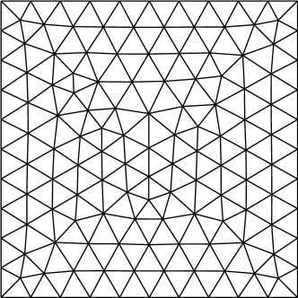
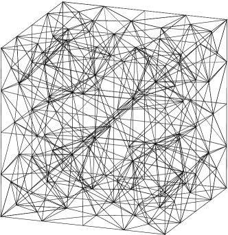
Figure 1. 2d triangular partition with $h=1/10$ (left) / 3d tetrahedral partition with $h=1/4$ (right).

Example 1. First, we consider a smooth problem defined on the unit square domain $\Omega=(0,1)^{2}$. The exact solution for the Helmholtz equation is given by [29],

$$u(x,y)=\mathrm{e}^{\boldsymbol{\mathrm{i}}k(x\cos{\frac{\pi}{5}}+y\sin{\frac{\pi}{5}})},$$

where the source term $f$ and the Robin boundary data $g$ are chosen accordingly. To obtain the convergence order, we solve this problem on a series of shape-regular meshes with the mesh size $h=1/5$, $h=1/10$, $\ldots$, $1/40$, see Fig .1. The convergence histories with the wave number $k=1,2,8$ for the accuracy $m=1,2,3,4$ are present in Tab. 1, Tab. 2 and Tab. 3, respectively. From the numerical errors, we observe that the convergence order of the error under the energy norm $|\!|\!|u-u_{h},\boldsymbol{p}-\boldsymbol{p}_{h}|\!|\!|$ is $O(h^{m})$, which is consistent to the theoretical result in Section 3. In addition, for the $L^{2}$ errors, we can see that $\|u-u_{h}\|_{L^{2}(\Omega)}$ and $\|\boldsymbol{p}-\boldsymbol{p}_{h}\|_{L^{2}(\Omega)}$ converge to zero at the rate $O(h^{m+1})$ and $O(h^{m})$, respectively, as the mesh is refined. Due to the finite machine precision, the convergence order is lower than the expected result for the case $m=4$ with the finest mesh. The pollution effect occurs as the wavenumber $k$ increases, since all the errors between the numerical solution and the exact solution become larger.

$m$	mesh size	$1/5$	$1/10$	$1/20$	$1/40$	order
$1$	$|\!|\!|(u-u_{h},\boldsymbol{p}-\boldsymbol{p}_{h})|\!|\!|$	6.468e-2	3.240e-2	1.620e-2	8.095e-3	1.00
	$\|u-u_{h}\|_{L^{2}(\Omega)}$	2.382e-3	6.074e-4	1.532e-4	3.844e-5	2.00
	$\|\boldsymbol{p}-\boldsymbol{p}_{h}\|_{L^{2}(\Omega)}$	1.980e-2	1.008e-2	5.026e-3	2.498e-3	0.99
$2$	$|\!|\!|(u-u_{h},\boldsymbol{p}-\boldsymbol{p}_{h})|\!|\!|$	1.385e-3	3.492e-4	8.758e-5	2.193e-5	2.00
	$\|u-u_{h}\|_{L^{2}(\Omega)}$	1.905e-5	2.378e-6	2.968e-7	3.707e-8	3.00
	$\|\boldsymbol{p}-\boldsymbol{p}_{h}\|_{L^{2}(\Omega)}$	4.084e-4	1.082e-4	2.765e-5	6.981e-6	1.99
$3$	$|\!|\!|(u-u_{h},\boldsymbol{p}-\boldsymbol{p}_{h})|\!|\!|$	2.085e-5	2.624e-6	3.301e-7	4.145e-8	3.00
	$\|u-u_{h}\|_{L^{2}(\Omega)}$	2.407e-7	1.514e-8	9.533e-10	5.987e-11	4.00
	$\|\boldsymbol{p}-\boldsymbol{p}_{h}\|_{L^{2}(\Omega)}$	5.464e-6	7.259e-7	9.509e-8	1.227e-8	2.99
$4$	$|\!|\!|(u-u_{h},\boldsymbol{p}-\boldsymbol{p}_{h})|\!|\!|$	2.482e-7	1.552e-8	9.704e-10	1.756e-10	3.48
	$\|u-u_{h}\|_{L^{2}(\Omega)}$	2.250e-9	6.999e-11	2.191e-12	1.232e-12	4.72
	$\|\boldsymbol{p}-\boldsymbol{p}_{h}\|_{L^{2}(\Omega)}$	6.688e-8	4.229e-9	2.659e-10	1.330e-10	2.99

Table 1. Convergence history for Example 1 with $k=1$.

$m$	mesh size	$1/5$	$1/10$	$1/20$	$1/40$	order
$1$	$|\!|\!|(u-u_{h},\boldsymbol{p}-\boldsymbol{p}_{h})|\!|\!|$	2.803e-1	1.327e-1	6.520e-2	3.243e-2	1.00
	$\|u-u_{h}\|_{L^{2}(\Omega)}$	2.112e-2	5.557e-3	1.412e-3	3.550e-4	1.99
	$\|\boldsymbol{p}-\boldsymbol{p}_{h}\|_{L^{2}(\Omega)}$	4.890e-2	2.154e-2	1.024e-2	5.020e-3	1.10
$2$	$|\!|\!|(u-u_{h},\boldsymbol{p}-\boldsymbol{p}_{h})|\!|\!|$	1.109e-2	2.793e-3	7.006e-4	1.754e-4	2.00
	$\|u-u_{h}\|_{L^{2}(\Omega)}$	1.628e-4	1.937e-5	2.386e-6	2.970e-7	3.00
	$\|\boldsymbol{p}-\boldsymbol{p}_{h}\|_{L^{2}(\Omega)}$	1.629e-3	4.323e-4	1.106e-4	2.792e-5	1.99
$3$	$|\!|\!|(u-u_{h},\boldsymbol{p}-\boldsymbol{p}_{h})|\!|\!|$	3.340e-4	4.199e-5	5.281e-6	6.632e-7	3.00
	$\|u-u_{h}\|_{L^{2}(\Omega)}$	3.858e-6	2.424e-7	1.525e-8	9.578e-10	4.00
	$\|\boldsymbol{p}-\boldsymbol{p}_{h}\|_{L^{2}(\Omega)}$	4.395e-5	5.814e-6	7.609e-7	9.812e-8	2.99
$4$	$|\!|\!|(u-u_{h},\boldsymbol{p}-\boldsymbol{p}_{h})|\!|\!|$	7.939e-6	4.967e-7	3.104e-8	1.941e-9	3.99
	$\|u-u_{h}\|_{L^{2}(\Omega)}$	7.229e-8	2.242e-9	6.978e-11	2.367e-12	4.96
	$\|\boldsymbol{p}-\boldsymbol{p}_{h}\|_{L^{2}(\Omega)}$	1.067e-6	6.763e-8	4.236e-9	2.664e-10	3.99

Table 2. Convergence history for Example 1 with $k=2$.

$m$	mesh size	$1/5$	$1/10$	$1/20$	$1/40$	order
$1$	$|\!|\!|(u-u_{h},\boldsymbol{p}-\boldsymbol{p}_{h})|\!|\!|$	1.220e+1	9.277e+0	5.208e+0	1.963e+0	0.87
	$\|u-u_{h}\|_{L^{2}(\Omega)}$	7.373e-1	5.652e-1	3.170e-1	1.174e-1	0.87
	$\|\boldsymbol{p}-\boldsymbol{p}_{h}\|_{L^{2}(\Omega)}$	7.511e-1	5.715e-1	3.201e-1	1.193e-1	0.87
$2$	$|\!|\!|(u-u_{h},\boldsymbol{p}-\boldsymbol{p}_{h})|\!|\!|$	2.916e+0	3.122e-1	4.786e-2	1.127e-2	2.66
	$\|u-u_{h}\|_{L^{2}(\Omega)}$	1.753e-1	1.586e-2	1.048e-3	6.796e-5	3.76
	$\|\boldsymbol{p}-\boldsymbol{p}_{h}\|_{L^{2}(\Omega)}$	1.772e-1	1.724e-2	2.041e-3	4.507e-4	2.90
$3$	$|\!|\!|(u-u_{h},\boldsymbol{p}-\boldsymbol{p}_{h})|\!|\!|$	1.066e-1	1.084e-2	1.353e-3	1.698e-4	3.10
	$\|u-u_{h}\|_{L^{2}(\Omega)}$	3.945e-3	9.116e-5	4.071e-6	2.463e-7	4.63
	$\|\boldsymbol{p}-\boldsymbol{p}_{h}\|_{L^{2}(\Omega)}$	4.905e-3	3.859e-4	4.888e-5	6.281e-6	3.23
$4$	$|\!|\!|(u-u_{h},\boldsymbol{p}-\boldsymbol{p}_{h})|\!|\!|$	8.138e-3	5.083e-4	3.180e-5	1.987e-6	4.00
	$\|u-u_{h}\|_{L^{2}(\Omega)}$	7.508e-5	1.828e-6	5.472e-8	1.688e-9	5.14
	$\|\boldsymbol{p}-\boldsymbol{p}_{h}\|_{L^{2}(\Omega)}$	2.777e-4	1.753e-5	1.105e-6	6.919e-8	3.99

Table 3. Convergence history for Example 1 with $k=8$.

Example 2. For the second example, we consider a 2d example defined on $\Omega=(-0.5,0.5)^{2}$ [17],

$$\left\{\begin{array}[]{ll}-\Delta u-k^{2}u&=f:=\frac{\sin(kr)}{r},\qquad\text{in }\Omega,\\ \frac{\partial{u}}{\partial\boldsymbol{\mathrm{n}}}+\boldsymbol{\mathrm{i}}ku&=g,\qquad\text{on }\partial\Omega.\end{array}\right.$$

The analytical solution can be written as

$$u=\frac{\cos(kr)}{k}-\frac{\cos k+\boldsymbol{\mathrm{i}}\sin k}{k(J_{0}(k)+\boldsymbol{\mathrm{i}}J_{1}(k))}J_{0}(kr),$$

in the polar coordinates $(r,\theta)$, where $J_{v}(z)$ are Bessel functions of the first kind.

First, we test the convergence order for the case $k=1$. We set the initial mesh size to be $h=1/5$ and uniformly refine the mesh for three times to solve this problem. The numerical errors are shown in Tab. 4 with the degree of approximation spaces $m=1,2,3$. We observe that the numerical error under the energy norm tends to zero at the speed $O(h^{m})$ as the mesh size approachs to zero, and the convergence order of $L^{2}$ errors are $O(h^{m+1})$ for the variable $u$ and $O(h^{m})$ for the varible $\boldsymbol{p}$. We note that all these results are still consistent with the theoretical error estimates. Fig. 2 exhibits the surface plots of the exact solution and the numerical solution for $k=100$.

Next, we numerically examine the changes of the error under the energy norm when the wavenumber $k$ and the mesh size $h$ are correlated. We use piecewise linear spaces to approximate the variables $u$ and $\boldsymbol{p}$, so that the error estimate in Theorem 23 suggests that

$$|\!|\!|(u-u_{h},\boldsymbol{p}-\boldsymbol{p}_{h})|\!|\!|\leq Ck^{2}h(1+h+k^{2}h^{2})(1+k^{2}h^{2})^{\frac{1}{2}}(\|u\|_{H^{2}(\Omega)}+\|\boldsymbol{p}\|_{H^{2}(\Omega)}).$$

In Fig. 3, we plot the relative energy error of the discontinuous least squares method for $k$ and $h$ determined by $k^{2}h=1$. We see that the error gradually decreases and tends to be invariant when $k$ becomes large, which verifies our $k$-explicit error estimates.

$m$	mesh size	$1/5$	$1/10$	$1/20$	$1/40$	order
$1$	$|\!|\!|(u-u_{h},\boldsymbol{p}-\boldsymbol{p}_{h})|\!|\!|$	3.386e-2	1.692e-2	8.466e-3	4.234e-3	1.00
	$\|u-u_{h}\|_{L^{2}(\Omega)}$	1.848e-3	4.664e-4	1.170e-4	2.929e-5	1.99
	$\|\boldsymbol{p}-\boldsymbol{p}_{h}\|_{L^{2}(\Omega)}$	2.430e-3	1.763e-3	9.741e-4	4.993e-4	0.76
$2$	$|\!|\!|(u-u_{h},\boldsymbol{p}-\boldsymbol{p}_{h})|\!|\!|$	1.135e-3	2.841e-4	7.106e-5	1.777e-5	2.00
	$\|u-u_{h}\|_{L^{2}(\Omega)}$	6.182e-6	7.257e-7	8.910e-8	1.107e-8	3.03
	$\|\boldsymbol{p}-\boldsymbol{p}_{h}\|_{L^{2}(\Omega)}$	9.629e-5	2.723e-5	7.185e-6	1.839e-6	1.90
$3$	$|\!|\!|(u-u_{h},\boldsymbol{p}-\boldsymbol{p}_{h})|\!|\!|$	1.543e-5	1.938e-6	2.428e-7	3.039e-8	3.00
	$\|u-u_{h}\|_{L^{2}(\Omega)}$	2.622e-7	1.633e-8	1.022e-9	6.403e-11	4.00
	$\|\boldsymbol{p}-\boldsymbol{p}_{h}\|_{L^{2}(\Omega)}$	1.778e-6	2.772e-7	3.738e-8	4.845e-9	2.83

Table 4. Convergence history for Example 2 with $k=1$.

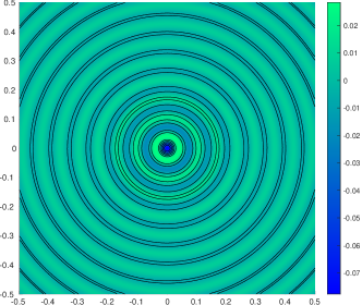
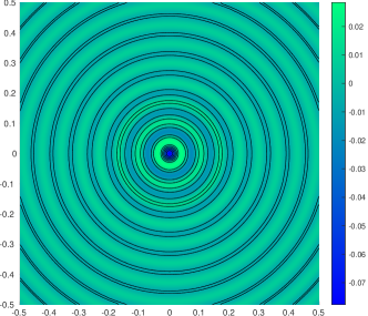
Figure 2. Surface plots for the exact solution of Example 2 (left) and the numerical solution with $k=100$ and $m=3$ (right). The number of elements is 139264.

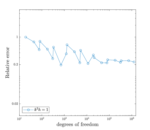
Figure 3. Relative error of Example 2 with $k^{2}h=1$.

Example 3. In this example, we solve a three-dimensional problem defined in the cube $\Omega=(-1,1)^{3}$. The analytical solution is selected as

$$u(x,y,z)=\mathrm{e}^{\boldsymbol{\mathrm{i}}k(x\sin\theta\cos\phi+y\sin\theta\sin\phi+z\cos\theta)},$$

where the parameter $\theta$ and $\phi$ are set to be $\frac{\pi}{4}$ and $\frac{\pi}{5}$ respectively. We solve this test problem on a series of tetrahedral meshes with the resolution $h=1/4$, $1/8$, $1/16$, and $1/32$, see Fig. 1. We use the approximation spaces $\boldsymbol{\mathrm{V}}_{h}^{m}$ and $\boldsymbol{\mathrm{\Sigma}}_{h}^{m}$ to approximate $u$ and $\boldsymbol{p}$, respectively. The convergence histories for $k=1$ are displayed in Tab. 5. We obseve that the convergence order under the energy norm $|\!|\!|\cdot|\!|\!|$ is still the optimal order $O(h^{m})$, and the $L^{2}$ errors for $u$ and $\boldsymbol{p}$ are still $O(h^{m})$ and $O(h^{m+1})$, respectively. We note that all numerical convergence orders are consistent with the theoretical error estimate as before.

$m$	mesh size	$1/4$	$1/8$	$1/16$	$1/32$	order
$1$	$|\!|\!|(u-u_{h},\boldsymbol{p}-\boldsymbol{p}_{h})|\!|\!|$	1.940e-1	9.754e-2	4.898e-2	2.458e-2	0.99
	$\|u-u_{h}\|_{L^{2}(\Omega)}$	1.591e-2	4.333e-3	1.117e-3	2.829e-4	1.94
	$\|\boldsymbol{p}-\boldsymbol{p}_{h}\|_{L^{2}(\Omega)}$	6.325e-2	3.538e-2	1.875e-2	9.595e-3	0.90
$2$	$|\!|\!|(u-u_{h},\boldsymbol{p}-\boldsymbol{p}_{h})|\!|\!|$	1.218e-2	3.181e-3	8.055e-4	2.030e-4	1.96
	$\|u-u_{h}\|_{L^{2}(\Omega)}$	4.952e-4	6.136e-5	7.612e-6	9.542e-7	3.00
	$\|\boldsymbol{p}-\boldsymbol{p}_{h}\|_{L^{2}(\Omega)}$	3.781e-3	1.194e-3	3.209e-4	8.287e-5	1.83
$3$	$|\!|\!|(u-u_{h},\boldsymbol{p}-\boldsymbol{p}_{h})|\!|\!|$	5.628e-4	7.438e-5	9.458e-6	1.198e-6	2.95
	$\|u-u_{h}\|_{L^{2}(\Omega)}$	1.770e-5	1.153e-6	7.299e-8	4.618e-9	3.96
	$\|\boldsymbol{p}-\boldsymbol{p}_{h}\|_{L^{2}(\Omega)}$	1.741e-4	2.808e-5	3.818e-6	4.991e-7	2.81

Table 5. Convergence history for Example 3 with $k=1$.

Example 4. In this test, we apply the proposed method to a problem with low regularity near the origin. The domain $\Omega$ is selected to be an L-shaped domain $\Omega=(-1,1)\backslash[0,1)\times(-1,0]$. We set $f=0$ and choose the exact solution, in polar coordinates $(r,\theta)$, to be

$$u(x,y)=J_{\alpha}(kr)\cos(\alpha\theta).$$

This exact solution belongs to the space $H^{\alpha+1-\epsilon}(\Omega)$. We select the parameter $\alpha=2/3$ and set the initial mesh size to be $h=1/4$. We uniformly refine the mesh for three times to solve this problem for $k=1$. Tab. 6 shows the convergence rate of $\|u-u_{h}\|_{L^{2}(\Omega)}$ and $\|\boldsymbol{p}-\boldsymbol{p}_{h}\|_{L^{2}(\Omega)}$ with $m=1,2,3$. The convergence rate of $\|\boldsymbol{p}-\boldsymbol{p}_{h}\|_{L^{2}(\Omega)}$ is about $0.67$, which is in agreement with with the regularity of the exact solution and error estimates. For the error $\|u-u_{h}\|_{L^{2}(\Omega)}$, we note that the convergence rate is lower than its regularity exponent, and seems to decrease when $m$ increases.

$m$	mesh size	$1/4$	$1/8$	$1/16$	$1/32$	order
$1$	$\|u-u_{h}\|_{L^{2}(\Omega)}$	1.019e-2	3.307e-3	1.109e-3	3.872e-4	1.57
	$\|\boldsymbol{p}-\boldsymbol{p}_{h}\|_{L^{2}(\Omega)}$	8.031e-2	4.900e-2	3.061e-2	1.920e-2	0.67
$2$	$\|u-u_{h}\|_{L^{2}(\Omega)}$	1.292e-3	4.483e-4	1.641e-4	6.226e-5	1.45
	$\|\boldsymbol{p}-\boldsymbol{p}_{h}\|_{L^{2}(\Omega)}$	4.023e-2	2.619e-2	1.652e-2	1.041e-2	0.66
$3$	$\|u-u_{h}\|_{L^{2}(\Omega)}$	7.098e-4	2.677e-4	1.032e-4	4.309e-5	1.37
	$\|\boldsymbol{p}-\boldsymbol{p}_{h}\|_{L^{2}(\Omega)}$	2.073e-2	1.706e-2	1.075e-2	6.776e-3	0.66

Table 6. Convergence history for Example 4 with $k=1$.

Example 5. In this example, we consider a circumferentially harmonic radiation from a rigid infinite circular cylinder of radius $a$ [20]. The exact solution is chosen by

(32) $$u(x,y)=\frac{H^{(1)}_{n}(kr)\cos n\theta}{H^{(1)}_{n}(ka)},$$

where $H^{(1)}_{n}$ is the Hankel function of the first kind of order $n$. The domain is set to be a circular ring $\Omega=B(0,2a)/B(0,a)$. We apply the Dirichlet boundary condition on $\partial B(0,a)$ and the Robin boundary condition on $\partial B(0,2a)$. In our numerical simulation, we compute the fifth circumferential mode ($n=4$) and choose $k=\pi$, $a=1$. We use the discontinuous piecewise linear approximation spaces $\boldsymbol{\mathrm{V}}_{h}^{1}\times\boldsymbol{\mathrm{\Sigma}}_{h}^{1}$ for this example. We use the polygon approximation to the domain $\Omega$, and then triangulate it into a shape-regular mesh, see Fig. 4 . In Fig. 5, we show the contours of the real part of the numerical solution and the exact solution, respectively. We observe that the least squres discontinuous finite element solution recovers the essential features of the exact solution.

Figure 4. The mesh used in Example 5 with 8908 elements.

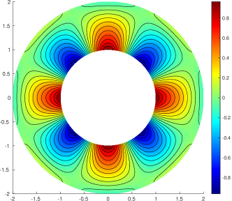
Figure 5. The real part of the numerical solution (left) and the exact solution (right) with $a=1$, $k=\pi$ and $m=1$.

Example 6. In this example, we test the performance of our adaptive algorithm proposed in Section 3. We solve the low-regularity problem defined in Example 4 with $\alpha=2/3$. For the adaptive algorithm, we choose the parameter $\lambda=0.45$ and we use the longest-edge bisection algorithm to refine the mesh. We use approximation spaces with $m=1$ to solve the problem. In Fig. 6, we compare the original mesh (left) with the mesh after 5 adaptive refinement steps (right). The mesh is refined remarkably around the corner $(0,0)$, where the exact solution contains a singularity. The convergence history under $L^{2}$ norms is displayed in Fig. 7. From Fig. 7, we see that the convergence orders of $\|u-u_{h}\|_{L^{2}(\Omega)}$ and $\|\boldsymbol{p}-\boldsymbol{p}_{h}\|_{L^{2}(\Omega)}$ are $O(N^{-1})$ and $O(N^{-1/2})$ , respectively, where $N$ is the number of degrees of freedom. These results match the convergence rates for smooth cases in Example 1 and Example 2. The convergence rates are better than that in Tab. 6, where the $L^{2}$ errors tend to zero at the speed $O(N^{-1.57/2})$ and $O(N^{-0.67/2})$ for the variables $u$ and $\boldsymbol{p}$, respectively.

Figure 6. The initial mesh (left) / The mesh after 5 adaptive refinement steps (right)

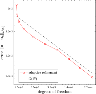
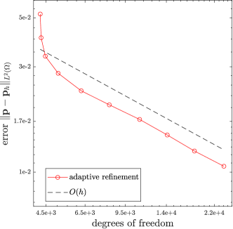
Figure 7. Convergence history for Example 6.

5. Conclusions

We proposed a discontinuous least squares finite element method for the Helmholtz equation. We designed an $L^{2}$ norm least squares functional with the weak imposition of the continuity across the interior faces, and minimized it over the discontinuous approximation space $\boldsymbol{\mathrm{V}}_{h}^{m}\times\boldsymbol{\mathrm{\Sigma}}_{h}^{m}$. We established the $k$-explicit error estimates for our method. The convergence rates were derived to be optimal under the energy norm and suboptimal under the $L^{2}$ norm for a fixed wavenumber $k$. Particularly, it was proved that our method is stable without any constraint on the mesh size. Numerical results in both two and three dimensions verified the accuracy of our method.

References

• [1] D. N. Arnold, F. Brezzi, B. Cockburn, and L. D. Marini, Unified analysis of discontinuous Galerkin methods for elliptic problems, SIAM J. Numer. Anal. 39 (2001/02), no. 5, 1749–1779.
• [2] I. Babuška and S. A. Sauter, Is the pollution effect of the FEM avoidable for the Helmholtz equation considering high wave numbers?, SIAM Rev. 42 (2000), no. 3, 451–484, Reprint of SIAM J. Numer. Anal. 34 (1997), no. 6, 2392–2423 [ MR1480387 (99b:65135)].
• [3] R. Bensow and M. G. Larson, Discontinuous least-squares finite element method for the div-curl problem, Numer. Math. 101 (2005), no. 4, 601–617.
• [4] R. E. Bensow and M. G. Larson, Discontinuous/continuous least-squares finite element methods for elliptic problems, Math. Models Methods Appl. Sci. 15 (2005), no. 6, 825–842.
• [5] P. Bochev, James Lai, and Luke Olson, A locally conservative, discontinuous least-squares finite element method for the Stokes equations, Internat. J. Numer. Methods Fluids 68 (2012), no. 6, 782–804.
• [6] P. B. Bochev and M. D. Gunzburger, Finite element methods of least-squares type, SIAM Rev. 40 (1998), no. 4, 789–837.
• [7] D. Boffi, F. Brezzi, and M. Fortin, Mixed Finite Element Methods and Applications, Springer Series in Computational Mathematics, vol. 44, Springer, Heidelberg, 2013.
• [8] F. Brezzi, J. J. Douglas, and L. D. Marini, Two families of mixed finite elements for second order elliptic problems, Numer. Math. 47 (1985), no. 2, 217–235.
• [9] F. Brezzi and M. Fortin, Mixed and hybrid finite element methods, Springer Series in Computational Mathematics, vol. 15, Springer-Verlag, New York, 1991.
• [10] C. L. Chang, A least-squares finite element method for the Helmholtz equation, Comput. Methods Appl. Mech. Engrg. 83 (1990), no. 1, 1–7.
• [11] H. Chen, P. Lu, and X. Xu, A hybridizable discontinuous Galerkin method for the Helmholtz equation with high wave number, SIAM J. Numer. Anal. 51 (2013), no. 4, 2166–2188. MR 3082496
• [12] H. Chen and W. Qiu, A first order system least squares method for the Helmholtz equation, J. Comput. Appl. Math. 309 (2017), 145–162.
• [13] P. G. Ciarlet, The Finite Element Method for Elliptic Problems, Classics in Applied Mathematics, vol. 40, Society for Industrial and Applied Mathematics (SIAM), Philadelphia, PA, 2002, Reprint of the 1978 original [North-Holland, Amsterdam; MR0520174 (58 #25001)].
• [14] S. Congreve, J. Gedicke, and I. Perugia, Robust adaptive $hp$ discontinuous Galerkin finite element methods for the Helmholtz equation, SIAM J. Sci. Comput. 41 (2019), no. 2, A1121–A1147. MR 3937921
• [15] B. Engquist and A. Majda, Radiation boundary conditions for acoustic and elastic wave calculations, Comm. Pure Appl. Math. 32 (1979), no. 3, 314–358.
• [16] C. Farhat, I. Harari, and U. Hetmaniuk, A discontinuous Galerkin method with Lagrange multipliers for the solution of Helmholtz problems in the mid-frequency regime, Comput. Methods Appl. Mech. Engrg. 192 (2003), no. 11-12, 1389–1419.
• [17] X. Feng and H. Wu, Discontinuous Galerkin methods for the Helmholtz equation with large wave number, SIAM J. Numer. Anal. 47 (2009), no. 4, 2872–2896.
• [18] by same author, $hp$-discontinuous Galerkin methods for the Helmholtz equation with large wave number, Math. Comp. 80 (2011), no. 276, 1997–2024.
• [19] X. Feng and Y. Xing, Absolutely stable local discontinuous Galerkin methods for the Helmholtz equation with large wave number, Math. Comp. 82 (2013), no. 283, 1269–1296.
• [20] I. Harari and T. J. R. Hughes, Galerkin/least-squares finite element methods for the reduced wave equation with nonreflecting boundary conditions in unbounded domains, Comput. Methods Appl. Mech. Engrg. 98 (1992), no. 3, 411–454.
• [21] U. Hetmaniuk, Stability estimates for a class of Helmholtz problems, Commun. Math. Sci. 5 (2007), no. 3, 665–678.
• [22] R. Hiptmair, A. Moiola, and I. Perugia, Plane wave discontinuous Galerkin methods for the 2D Helmholtz equation: analysis of the $p$-version, SIAM J. Numer. Anal. 49 (2011), no. 1, 264–284. MR 2783225
• [23] R. H. W. Hoppe and N. Sharma, Convergence analysis of an adaptive interior penalty discontinuous Galerkin method for the Helmholtz equation, IMA J. Numer. Anal. 33 (2013), no. 3, 898–921. MR 3081488
• [24] P. Houston, I. Perugia, and D. Schneebeli, A.and Schötzau, Interior penalty method for the indefinite time-harmonic Maxwell equations, Numer. Math. 100 (2005), no. 3, 485–518.
• [25] Q. Hu and R. Song, A novel least squares method for Helmholtz equations with large wave numbers, SIAM J. Numer. Anal. 58 (2020), no. 5, 3091–3123.
• [26] F. Ihlenburg and I. Babuška, Finite element solution of the Helmholtz equation with high wave number. I. The $h$-version of the FEM, Comput. Math. Appl. 30 (1995), no. 9, 9–37.
• [27] by same author, Finite element solution of the Helmholtz equation with high wave number. II. The $h$-$p$ version of the FEM, SIAM J. Numer. Anal. 34 (1997), no. 1, 315–358.
• [28] O. A. Karakashian and F. Pascal, A posteriori error estimates for a discontinuous Galerkin approximation of second-order elliptic problems, SIAM J. Numer. Anal. 41 (2003), no. 6, 2374–2399.
• [29] B. Lee, T. A. Manteuffel, S. F. McCormick, and J. Ruge, First-order system least-squares for the Helmholtz equation, SIAM J. Sci. Comput. 21 (2000), no. 5, 1927–1949.
• [30] R. Li, Q. Liu, and F. Yang, A discontinuous least squares finite element for time-harmonic Maxwell equations, accepted by IMA J. Numer. Anal. (2020).
• [31] R. Li and F. Yang, A least squares method for linear elasticity using a patch reconstructed space, Comput. Methods Appl. Mech. Engrg. 363 (2020), no. 1, 112902.
• [32] J. M. Melenk and S. Sauter, Wavenumber explicit convergence analysis for Galerkin discretizations of the Helmholtz equation, SIAM J. Numer. Anal. 49 (2011), no. 3, 1210–1243.
• [33] P. Monk and D.-Q. Wang, A least-squares method for the Helmholtz equation, Comput. Methods Appl. Mech. Engrg. 175 (1999), no. 1-2, 121–136. MR 1692914
• [34] N. C. Nguyen, J. Peraire, F. Reitich, and B. Cockburn, A phase-based hybridizable discontinuous Galerkin method for the numerical solution of the Helmholtz equation, J. Comput. Phys. 290 (2015), 318–335.
• [35] P.-A. Raviart and J. M. Thomas, A mixed finite element method for 2nd order elliptic problems, Mathematical aspects of finite element methods (Proc. Conf., Consiglio Naz. delle Ricerche (C.N.R.), Rome, 1975), 1977, pp. 292–315. Lecture Notes in Math., Vol. 606.
• [36] L. L. Thompson and P. M. Pinsky, A Galerkin least-squares finite element method for the two-dimensional Helmholtz equation, Internat. J. Numer. Methods Engrg. 38 (1995), no. 3, 371–397.