Analytical results for a minimalist thermal diode

Abstract

We consider a system consisting of two interacting classical particles, each one subject to an on-site potential and to a Langevin thermal bath. We analytically calculate the heat current that can be established through the system when the bath temperatures are different, for weak nonlinear forces. We explore the conditions under which the diode effect emerges when inverting the temperature difference. Despite the simplicity of this two-particle diode, an intricate dependence on the system parameters is put in evidence. Moreover, behaviors reported for long chains of particles can be extracted, for instance, the dependence of the flux with the interfacial stiffness and type of forces present, as well as the dependencies on the temperature required for rectification. These analytical results can be a tool to foresee the distinct role that diverse types of nonlinearity and asymmetry play in thermal conduction and rectification.

I Introduction

Simplified microscopic models, such as classical particle chains in contact with heat baths, have proven useful to grasp the physics of thermal transport in low dimensions fourier ; ReviewLepriLiviPoliti2003 ; ReviewDhar2008 ; LepriBook2016 . The interest in one-dimensional models goes beyond the theoretical challenge to derive the laws of heat conduction from the microscopic dynamics, insofar as they can be useful for understanding the anomalies observed in real systems, such as carbon nanotubes nano2008 , nanowires YangZhangLi2010 , and molecular chains chain1 ; chain2 . Moreover, these experiments and theories can lead to the development of new technologies for heat flow manipulation e1 . An interesting example is the thermal diode, whose thermal conductivity along a given axis changes depending on the direction of the heat flux, yielding rectification in a preferential direction. This proposal, initially conceived through simplified theoretical modeling  casati-diode , soon found materialization in solid-state experiments exp-diode .

Subsequently, several variants of microscopic models were proposed to determine the conditions to achieve efficient rectification, by analyzing for instance the effects of the range of the interactions or graded masses efficiency1 ; efficiency2 , the role of the interface interface ; pons2017 ; efficiency3 ; BaowenLi2005 ; BaowenLi2011 , among others. In the meantime, several efforts have been directed towards an analytical understanding of the diode effect, putting into evidence the requirements of asymmetry and nonlinearity for rectification, for instance, by linearizing the equations of motion but, as counterpart, making the parameters along a mass graded chain temperature dependent Tdependence . Closely related, in a very recent work, the diode effect was shown in the so-called temperature-gradient harmonic oscillator chains harmonic . In the same spirit, a minimalistic model of two harmonic oscillators with temperature dependency has been recently studied Muga2021 . The two-segment chain of classical spins in contact with multiple heat baths has also been studied spins , as well as quantum systems, to show rectification of the heat flow between two thermal baths through a pair of interacting qubits quantum-diode or even quantum spin chains perfectdiode .

Here, we investigate a minimalist model of only two interacting classical particles connected to heat baths, in order to understand the diode effect directly from the equations of motion. We solve these equations in the limit of small nonlinearity, from a perturbative approach. Then, we obtain expressions for the heat flow and rectification factor allowing us to directly grasp the impact of asymmetries and nonlinearities, as well as qualitative features of heat conduction and rectification, explicitly expressed in terms of the model parameters.

The paper is organized as follows. The system is defined in Sec. II. The perturbative solution and associated heat flow are described in Secs. III and IV, respectively, while the mathematical derivations can be found in the Appendix. The diode effect is discussed in Sec. V with final remarks in Sec. VI.

Figure 1: Schematic representation of a minimalist thermal diode.

II The system

We consider a one-dimensional system composed of two particles, with masses $m_{j}$ (with $j=A,B$), coordinates $x$ and $y$, subject to on-site potentials $V_{j}$ and interacting through a potential $V_{I}$ such that the complete Hamiltonian is

$$\mathcal{H}=\frac{p_{A}^{2}}{2m_{A}}+V_{A}(x)+\frac{p_{B}^{2}}{2m_{B}}+V_{B}(y)+V_{I}(x-y).$$ (1)

Moreover, each particle $j$ is put in contact with a Langevin thermal bath at temperature $T_{j}$. A pictorial representation of this kind of system is provided in Fig. 1. Let us remark that this system is very similar to the couple of harmonic oscillators recently investigated Muga2021 , but in our case we introduce nonlinear forces. Namely, we treat the case where the interaction potential is harmonic with stiffness $k_{I}$, while the on-site potential of particle $j$ is $V_{j}(z)=k_{j}z^{2}/2+\epsilon V^{nl}_{j}(z)$, where $k_{j}$ is the harmonic stiffness and $f_{j}(z)=-dV^{nl}_{j}(z)/dz$ is an arbitrary nonlinear force, whose intensity is controlled by the unitless constant $\epsilon$. Explicitly, the equations of motion are

$$m_{A}\ddot{x}+\gamma_{A}\dot{x}+k_{A}x+k_{I}(x-y) = \epsilon f_{A}(x)+\eta_{A}(t),$$ (2)

$$m_{B}\ddot{y}+\gamma_{B}\dot{y}+k_{B}y+k_{I}(y-x) = \epsilon f_{B}(y)+\eta_{B}(t)\,,$$ (3)

where $\epsilon$ is a dimensionless parameter that controls the strength of the nonlinear forces, $\gamma_{j}$ is the damping coefficient and $\eta_{j}$ the fluctuating force of the Langevin thermostat $j$ ($j=A,B$), where $\eta_{A}$ and $\eta_{B}$ are independent zero-mean Gaussian-distributed white noises with

$$\langle\eta_{A}(t)\eta_{A}(t^{\prime})\rangle = 2\gamma_{A}T_{A}\delta(t-t^{\prime}),$$

$$\langle\eta_{B}(t)\eta_{B}(t^{\prime})\rangle = 2\gamma_{B}T_{B}\delta(t-t^{\prime})\,,$$

where the temperature is in units of the Boltzmann constant. Although we might suppress some parameters by fixing space and timescales, we will keep them explicit to preserve the AB symmetry of the equations.

III Perturbative solution

Eqs. (2)-(3) cannot be solved exactly, however, if $\epsilon$ is small enough to ensure that the energy stored in the nonlinear mode is much smaller than in the harmonic one, we can expand the coordinates as

$$x(t) = x_{0}(t)+\epsilon\,x_{1}(t)+\mathcal{O}(\epsilon^{2}),$$ (4)

$$y(t) = y_{0}(t)+\epsilon\,y_{1}(t)+\mathcal{O}(\epsilon^{2}),$$ (5)

where the zeroth-order terms follow the equations

$$m_{A}\ddot{x}_{0}+\gamma_{A}\dot{x}_{0}+k_{A}x_{0}+k_{I}(x_{0}-y_{0}) = \eta_{A}(t),$$ (6)

$$m_{B}\ddot{y}_{0}+\gamma_{B}\dot{y}_{0}+k_{B}y_{0}+k_{I}(y_{0}-x_{0}) = \eta_{B}(t),$$ (7)

which are linear and uncoupled equations, and the first-order corrections $x_{1}$ and $y_{1}$ follow

$$m_{A}\ddot{x}_{1}+\gamma_{A}\dot{x}_{1}+k_{A}x_{1}+k_{I}(x_{1}-y_{1}) = f_{A}(x_{0})\,,$$ (8)

$$m_{B}\ddot{y}_{1}+\gamma_{B}\dot{y}_{1}+k_{B}y_{1}+k_{I}(y_{1}-x_{1}) = f_{B}(y_{0}).$$ (9)

Since we are interested in the long-time behavior, the initial conditions are not relevant, therefore we will use the Fourier transform, defined as $\tilde{z}(\omega)=\int_{-\infty}^{\infty}dt\,z(t)\,{e}^{-i\omega t}$, to solve the above stochastic differential equations. We start by expressing Eqs. (6)-(7) in Fourier space, namely,

$$\underbrace{\big{(}k_{A}+k_{I}-m_{A}\omega^{2}+i\gamma_{A}\omega\big{)}}_{\displaystyle a(\omega)}\tilde{x}_{0}-k_{I}\tilde{y}_{0} = \tilde{\eta}_{A}(\omega)\,,$$ (10)

$$\underbrace{\big{(}k_{B}+k_{I}-m_{B}\omega^{2}+i\gamma_{B}\omega\big{)}}_{\displaystyle b(\omega)}\tilde{y}_{0}-k_{I}\tilde{x}_{0} = \tilde{\eta}_{B}(\omega)\,,$$ (11)

whose solution in matrix form is

$$\begin{pmatrix}\tilde{x}_{0}(\omega)\\ \tilde{y}_{0}(\omega)\end{pmatrix}=\frac{\begin{pmatrix}b(\omega)&k_{I}\\ k_{I}&a(\omega)\end{pmatrix}\begin{pmatrix}\tilde{\eta}_{A}(\omega)\\ \tilde{\eta}_{B}(\omega)\end{pmatrix}}{a(\omega)b(\omega)-k_{I}^{2}}\,.$$ (12)

Similarly, solving Eqs. (8) and (9) in Fourier space, we obtain (for more details see A1)

$$\begin{pmatrix}\tilde{x}_{1}(\omega)\\ \tilde{y}_{1}(\omega)\end{pmatrix}=\frac{\begin{pmatrix}b(\omega)&k_{I}\\ k_{I}&a(\omega)\end{pmatrix}\begin{pmatrix}\mathcal{F}\left\{f_{A}({x}_{0})\right\}(\omega)\\ \mathcal{F}\left\{f_{B}({y}_{0})\right\}(\omega)\end{pmatrix}}{a(\omega)b(\omega)-k_{I}^{2}}\,.$$ (13)

IV Heat flow

The heat flow $J$ along the system can be defined in several forms that are equivalent when the system reaches a stationary state (see for instance ReviewDhar2008 ). The potential $V_{I}(x-y)$ represents the energy stored in the interaction between neighboring particles, and the energetic flow can be written as

$$\frac{d}{dt}\big{\langle}V_{I}(x-y)\big{\rangle} = \big{\langle}V^{\prime}_{I}(x-y)\dot{x}\big{\rangle}-\big{\langle}V^{\prime}_{I}(x-y)\dot{y}\big{\rangle},$$

and, under stationarity, $\langle V^{\prime}_{I}(x-y)\dot{x}\rangle=\langle V^{\prime}_{I}(x-y)\dot{y}\rangle$. From this identity, we have equivalent definitions that in our case, where $V_{I}^{\prime}(x-y)=k_{I}(x-y)$, read

$$J = \langle k_{I}(x-y)\dot{x}\rangle=\langle k_{I}(x-y)\dot{y}\rangle\,,$$ (14)

or still $J=\langle k_{I}(x-y)(\dot{x}+\dot{y})/2\rangle$. The heat flow $J$ can also be expanded in a series of $\epsilon$, as

$$J = J_{0}+\epsilon J_{1}+O(\epsilon^{2})\,.$$ (15)

In the linear regime, Eq. (14) yields (see Appendix A2)

$$J_{0} = k_{I}\langle x_{0}\dot{x}_{0}\rangle-k_{I}\langle y_{0}\dot{x}_{0}\rangle$$ (16)

$$= -k_{I}\int\frac{d\omega d\omega^{\prime}}{(2\pi)^{2}}e^{it(\omega+\omega^{\prime})}\langle\tilde{y}_{0}(\omega)\;i\omega^{\prime}\;\tilde{x}_{0}(\omega^{\prime})\rangle\,.\;\;\;$$ (17)

Then, we obtain

$$J_{0} = \kappa_{0}\big{(}T_{A}-T_{B}\big{)}\,,$$ (18)

where the zeroth-order thermal conductivity is

$$\kappa_{0} = \int\frac{d\omega}{2\pi}\frac{2\gamma^{2}k_{I}^{2}\omega^{2}}{|a(\omega)b(\omega)-k_{I}^{2}|^{2}}\,.$$ (19)

Note: This expression shows that, regardless of the asymmetries that may be present, the linear system cannot be converted to a thermal diode since $\kappa_{0}$ does not depend on the temperatures and it is invariant under particle exchange, hence, the magnitude of the flow is the same in both directions.

With regard to the dependence of $\kappa_{0}$ on the coupling strength $k_{I}$, Eq. (19) gives $\kappa_{0}\sim k_{I}^{2}+O(k_{I}^{3})$, for small $k_{I}$. It is interesting to note that this is the scaling observed for two-segment chains with nonlinear forces of Frenkel-Kontorova (FK) type casati-diode .

Now we proceed to calculate the first-order correction of the current $J$, containing the information on the nonlinearities. From Eq. (14), we have

$$J = -k_{I}\langle y(t)\dot{x}(t)\rangle=$$ (20)

$$= \underbrace{-k_{I}\langle y_{0}\dot{x}_{0}\rangle}_{\displaystyle J_{0}}+\epsilon\underbrace{(-k_{I})\{\langle y_{1}\dot{x}_{0}\rangle+\langle y_{0}\dot{x}_{1}\rangle\}}_{\displaystyle J_{1}}\,,$$

where the correlations in $J_{1}$ are calculated in Appendix A2, yielding $J_{1}=\kappa_{1}(T_{A},T_{B})\,\Delta T$, with

$$\kappa_{1}(T_{A},T_{B}) = \kappa_{0}\sum_{j=A,B}\beta_{j}\,g_{j}\big{(}\sigma_{mj}T_{m}+\sigma_{j}T_{j}\big{)},\;\;\;\;\;\;$$ (21)

where $T_{m}=(T_{A}+T_{B})/2$ is the mean temperature, $\beta_{j}$, $\sigma_{mj}$ and $\sigma_{j}$ ($j=A,B$) are coefficients that do not depend on the temperature (derived in Appendix A2, where explicit expressions are also given), and $g_{j}$ is derived from the Fourier transform of the force $f_{j}$ (for examples see Table I).

$f_{j}(z)=\sum_{n\geq 0}c_{j,n}z^{n}$	$g_{j}(z)=\sum_{n\geq 1}c_{j,n}\,n!!\,z^{(n-1)/2}$
$-z^{2n-1}$, $n\in\mathbb{N}$	$-(2n-1)!!\,z^{n-1}$
$-\sin(Kz)$	$-K{e}^{-K^{2}z/2}$
$-\sinh(Kz)$	$-K{e}^{K^{2}z/2}$

Table 1: Nonlinear force $f_{j}$ and associated function $g_{j}$ (derived in Appendix A2).

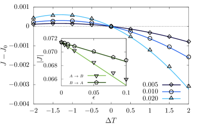
In Fig. 2, an illustrative example shows the good agreement between the first-order theoretical prediction, Eq. (20), and the numerical evaluation of Eq. (14), performed over trajectories obtained from the numerical integration of the equations of motion, using an eighth-order Runge-Kutta algorithm RK8 .

Figure 2: Heat current difference $J-J_{0}$ vs. $\Delta T$. Solid lines correspond to the theoretical prediction given by Eq. (20) and symbols to the computation from numerical integration of the equations of motion, averaged over $10^{5}$ realizations. $V_{A}^{nl}(z)=z^{4}/4$, $V_{B}^{nl}(z)=0$, Different values of $\epsilon$ indicated on the figure were considered, $k_{I}=0.5$ and all other parameters are equal to 1. The inset shows the current $|J|$ as a function of $\epsilon$ for $\Delta T=\pm 1$ (i.e, $A\rightleftarrows B$). (Color online.)

For weak coupling, the scaling

$$\kappa\sim k_{I}^{2}+O(k_{I}^{3},\epsilon k_{I}^{2})\,,$$ (22)

obtained in the linear case, still holds, while $\kappa$ tends to a constant value for large $k_{I}$. Of course, if the interfacial interaction, which connects the two units of the system, vanishes, hence, $\kappa$ vanishes too, as expected due to disruption of the channel for energy flux.

As a check of consistency, we verified that, if $f_{j}(z)$ were linear, then $g_{j}(z)$ would be a constant $\bar{g}_{j}<0$ ($n=0$ in Table I), in which case Eq. (21) becomes $\kappa_{1}=(\beta_{A}\bar{g}_{A}+\beta_{B}\bar{g}_{B})\,\kappa_{0}$  in accord with the zeroth order expression for $\kappa_{0}$, Eq. (19), after substituting $k_{A}\to k_{A}-\epsilon\bar{g}_{A}$ and $k_{B}\to k_{B}-\epsilon\bar{g}_{B}$.

Since the linear conductivity $\kappa_{0}$ does not depend on the bath temperatures, the heat flux will have the same magnitude in both directions. Therefore, for rectification, it is crucial that at least one of the two forces $f_{j}(z)$ be nonlinear. This nonlinearity would act by introducing a dependence of the conductivity on the temperatures, through the argument of $g_{j}(z)$ in Eq. (21), which originates from the correlations of the zeroth-order coordinates. A temperature dependence that is asymmetric under particle exchange is then responsible for thermal rectification, as discussed in the next section. Moreover, this is the basis of the diode effect on harmonic systems with imposed or natural temperature dependencies Tdependence ; harmonic ; Muga2021 .

V Diode effect

First, recall that $\beta_{j}$, $\sigma_{mj}$ and $\sigma_{j}$, which define $J_{1}$, are quantities that do not depend on the end temperatures. While $\sigma_{mj}$ (as well as $\kappa_{0}$) is always positive, $\beta_{j}$ and $\sigma_{j}$ have not definite sign in general, however, $\sigma_{mj}T_{m}+\sigma_{j}T_{j}$ must be positive. Moreover, in contrast to $\kappa_{0}$ and the $\sigma_{mj}$ whose expressions are invariant by AB-exchange, the coefficients $\beta_{j}$ or $\sigma_{j}$ may be non-symmetric in general, which would ensure that even if $g_{A}$ = $g_{B}$, the conductivity can become dependent on the direction of the flux.

Let us define the fluxes $J_{AB}$ and $J_{BA}$ for the positive temperature gradient ($T_{A}=T_{h}>T_{c}=T_{B}$) and the reversed one, as schematized in Fig. 1. From the expression of $J$, we have

$$J_{AB}\equiv J_{A\to B} = \big{[}\kappa_{0}+\epsilon\underbrace{\kappa_{1}(T_{h},T_{c})}_{\displaystyle\kappa_{1}^{AB}}\big{]}(T_{h}-T_{c}),$$

$$J_{BA}\equiv J_{B\to A} = \big{[}\kappa_{0}+\epsilon\underbrace{\kappa_{1}(T_{c},T_{h})}_{\displaystyle\kappa_{1}^{BA}}\big{]}(T_{c}-T_{h}).$$

Rectification emerges when $\kappa_{1}^{AB}\neq\kappa_{1}^{BA}$, molded by the functions $g_{j}(z)$, associated to nonlinear forces $f_{j}(z)$, which introduce the dependence of the conductivity on the bath temperatures.

In what follows, to quantify the diode effect, we use the ratio

$$\chi\equiv\frac{\big{|}|J_{AB}|-|J_{BA}|\big{|}}{\big{(}|J_{AB}|+|J_{BA}|\big{)}/2}=\epsilon\frac{|\kappa_{1}^{AB}-\kappa_{1}^{BA}|}{\kappa_{0}}+O(\epsilon^{2})\,.$$ (24)

This quantity coincides with the rectification factor casati-diode at first order in $\epsilon$ and it is twice the diodicity alexander . Notice that, the departure from the linear regime, signaled by $\epsilon\neq 0$, together with asymmetry, is required to allow the diode effect ($\chi\neq 0$) at first order in $\epsilon$. However, the rectification $\chi$ is small, of order $\epsilon$.

In the following sections, we will discuss the behavior of $\chi$ in some particular cases, in order to reduce the number of parameters.

V.1 Symmetric chain

Let us address the case where $k_{A}=k_{B}$, $m_{A}=m_{B}$ and $\gamma_{A}=\gamma_{B}$, hence, the asymmetry required for rectification must reside in the nonlinear on-site forces. In this simple case, the coefficients obtained in Appendix A2 reduce to

$$\sigma_{m} = \frac{[(k+k_{I})\bar{m}+1]k_{I}^{2}}{k(k+2k_{I})(k+k_{I}+\bar{m}k_{I}^{2})}\,,$$ (25)

$$\sigma_{A} = \sigma_{B}=\sigma=\frac{1}{k+k_{I}+\bar{m}k_{I}^{2}}\,,$$ (26)

$$\beta_{A} = \beta_{B}=\sigma/2.$$ (27)

Then,

$$\chi = \epsilon\frac{\big{|}g_{A}(T_{+})-g_{A}(T_{-})+g_{B}(T_{-})-g_{B}(T_{+})\big{|}}{2[k+k_{I}+\bar{m}k_{I}^{2}]}\,,$$ (28)

where $T_{\pm}=\sigma_{m}T_{m}+\sigma T_{\begin{subarray}{c}h\\[-2.0pt] c\end{subarray}}=(\sigma_{m}+\sigma)T_{m}\pm\sigma(T_{h}-T_{c})/2$.

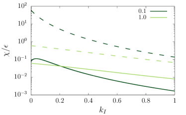
First, we notice that $\chi$ is finite in the limit $k_{I}\to 0$ and it tends to zero in the opposite limit $k_{I}\to\infty$. Examples are given in Fig. 3 for two different potentials.

Figure 3: Scaled rectification factor as a function of the interfacial stiffness $k_{I}$, for the nonlinear on-site potential $V_{A}^{nl}(z)=z^{4}/4$, (power-law, dashed lines), and $V_{A}^{nl}(z)=-\cos(z)$, (sinusoidal, solid lines), for $k=0.1$ (dark green) and 1 (light green), as indicated in the legend. In all cases $V_{B}^{nl}\equiv 0$, $\bar{m}=1$, $T_{m}=1$, $\Delta T=0.4$. (Color online.)

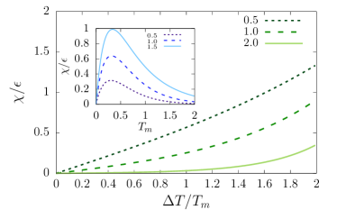
Rectification enhancement can be achieved by augmenting the temperature difference, fixing the average, since $\Delta g_{j}\equiv g_{j}(T^{+})-g_{j}(T^{-})\approx g_{j}^{\prime}([\sigma_{m}+\sigma]T_{m})\,\Delta T+{\cal O}([\Delta T]^{3})$. This effect is illustrated inf Fig. 4. As a matter of fact, the increase of the rectification factor with the temperature difference has been observed in diverse models efficiency2 ; efficiency3 ; bastida .

Figure 4: Scaled rectification factor as a function of the relative temperature difference $\Delta T/T_{m}$, for the nonlinear on-site potential $V_{A}^{nl}(z)=-\cos(z)$, $V_{B}^{nl}\equiv 0$, $k=k_{I}=0.1$, for different values of $T_{m}$, indicated in the legend. The inset displays the scaled rectification vs. $T_{m}$ for different values of $\Delta T$ indicated in the legend, showing that there is an optimal $T_{m}$, due to the loss of nonlinearity in the extremes of low and high temperatures for the chosen potential. (Color online.)

The mass and inverse square damping contribute trough $\bar{m}=m/\gamma^{2}$ to spoil rectification if $k_{I}>0$. This suggests that the overdamped regime would perform rectification better.

We can also understand how the preferential direction in which the conductivity is larger, for given bath temperatures, depends on the type of nonlinear forces. For instance, let us consider $g_{B}(z)=0$. If $g_{A}(z)$ is monotonically decreasing, like in the power-law case of Table I, then $\Delta g_{A}<0$, for $T_{A}>T_{B}$, indicating that the preferential direction is from B to A (in general from smaller to larger nonlinear force). However, if the potential is sinusoidal, $g_{A}(z)$ is an increasing function (Table I), then the preferential direction is inverted with respect to the previous case (i.e., it is from A to B), as observed for asymmetric FK chains casati-diode ).

Let us take a closer look to the conductivity in the limit $k_{I}\to 0$, for some concrete potentials $V_{A}^{nl}$, while $V_{B}^{nl}=0$. Recall that the conductivity scales with $k_{I}^{2}$, then the fluxes vanish in the limit $k_{I}\to 0$, however $\chi$ can be large for finite but very small $k_{I}$. In that limit, we have $\sigma_{m}=0$, $\sigma=1/k$, hence the scaled mass $\bar{m}$ does not play a role in the rectification.

For the power-law on-site potential $V_{A}^{nl}(z)=z^{2n}/(2n)$, $g_{A}(z)=-(2n-1)!!z^{n-1}$, with $n>1$, in the limit $k_{I}\to 0$, Eq. (28) becomes

$$\chi=\epsilon\frac{(2n-1)!!}{2k}\left[\left(\frac{T_{h}}{k}\right)^{n-1}-\left(\frac{T_{c}}{k}\right)^{n-1}\right]\,.$$ (29)

Equation (29) predicts, for instance, that the ratio $\chi$ grows with the temperature difference $\Delta T=T_{h}-T_{c}$, with positive concavity for $n>2$, nearly linear for small $\Delta T$. These effects persist for finite $k_{I}$ as shown in Fig. 4.

For the sinusoidal on-site potential $V_{A}^{nl}(z)=-\cos(Kz)/K$ (as in the FK model), $g_{A}(z)=-K{e}^{-K^{2}z/2}$ (see Table I). In this case the dependence $\chi$ vs. $k_{I}$ can be nonmonotonic, with a finite optimal value, as shown in Fig. 3. In the limit $k_{I}\to 0$ we obtain

$$\chi=\epsilon\frac{K}{2k}\left(e^{-K^{2}T_{c}/(2k)}-e^{-K^{2}T_{h}/(2k)}\right)\,.$$ (30)

The dependence on $\Delta T$ (for fixed mean temperature $T_{m}$) is also an increasing convex function. This behavior, which also holds for finite $k_{I}$, as exemplified in Fig. 4, is qualitatively similar to that reported from simulations of diode models efficiency2 ; efficiency3 ; bastida . For the power-law potential the nonlinear correction is weak but in the same direction.

V.2 Small $k_{I}$ limit

In the previous section, we have seen that the limit of small $k_{I}$ is relevant, while it allows to simplify the analytical expressions significantly. Then, in this limit, we will analyze the effect of introducing the asymmetry alternatively in the stiffness ($k_{A}\neq k_{B}$), mass ($m_{A}\neq m_{B}$) or damping coefficient ($\gamma_{A}\neq\gamma_{B}$). As shown in Appendix A3, in this limit,

$$\kappa_{1} \simeq \kappa_{0}\Big{[}\beta_{A}\,g_{A}(\sigma_{A}T_{A})+\beta_{B}\,g_{B}(\sigma_{B}T_{B})\Big{]}\,,$$ (31)

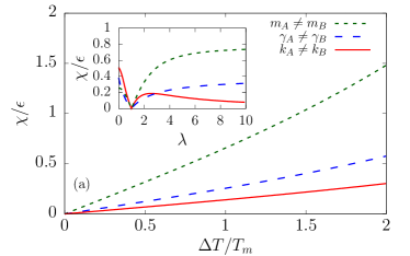
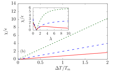
where the explicit expressions for the coefficients are given in the Appendix A3 for each asymmetry. The results for the rectification factor $\chi$ are illustrated in Fig. 5.

Note: We observe that any of these asymmetries can produce rectification. In particular, notice that, even when the chain is homogeneous, distinct thermostats (characterized by different friction coefficients) can also produce a diode effect.

Figure 5: Scaled rectification factor vs. the relative temperature difference $\Delta T/T_{m}$, with $T_{m}=1$, for nonlinear on-site potential $V_{A}^{nl}(z)=V_{B}^{nl}(z)=$ (a) $-\cos(z)$ and (b) $z^{4}/4$ for: $m_{A}=5$, $k_{A}=k_{B}=m_{B}=\gamma_{A}=\gamma_{B}=1$ (green), $\gamma_{A}=5$, $\gamma_{B}=k_{A}=k_{B}=m_{A}=m_{B}=1$ (blue) $k_{A}=5$, $k_{B}=m_{A}=m_{B}=\gamma_{A}=\gamma_{B}=1$ (red). The insets show the dependence on the asymmetry factor $\lambda$ that for each parameter $p$ gives $p_{A}=\lambda p_{B}=\lambda$. (Color online.)

VI Final remarks

We have presented analytical results starting from the microscopic classical dynamics of a two-particle system with nonlinear forces. Due to the nonlinearity of the equations, we tackled the solution from a perturbative approach valid for small nonlinear intensity $\epsilon$. It is noticeable that despite the simplicity of the system, the conductivity $\kappa=\kappa_{0}+\epsilon\kappa_{1}$ has an intricate dependence on the system parameters. Therefore, it might be hard to make a portrait of this complexity only through molecular dynamics simulations, making worthy the present effort of obtaining analytical results from first principles.

Some previously known results can be revisited from this perspective. Particularly, one can see how the temperature-dependence of the conductivity emerges from the nonlinearity of the forces, through the functions $g_{j}(z)$. The requirements of broken symmetry and of nonlinearity explicitly appear. The results also allow shedding light on effects observed in chains, e.g., the scaling of the conductivity with the interfacial stiffness $k_{I}$, the dependence of the rectification factor on $k_{I}$ and on the temperature difference. How nonlinearities determine the preferential direction has also been foreseen. The role of different asymmetries (in the mass, stiffness, on-site potential and even damping coefficient) was also shown.

It is interesting to note that, from Appendix A2, it is possible to obtain that the nonlinearity yields a temperature-dependent power spectrum (anharmonic phonons), which can be seen as the correction to the harmonic theory responsible for phonon scattering hanggi . The relationship between temperature and the overlapping phonon bands has already been analytically studied for FK asymmetric chains casati-diode and chains with dissimilar anharmonic segments (FK and Fermi-Pasta-Ulan-Tsingou)  casati-diode ; BaowenLi2005 .

Our results are valid when the effect of the nonlinear forces can be treated as a perturbation to the predominantly linear solutions. Consequently, the predicted diode effect is very small. However, the results allow for a clear glance regarding the mechanisms behind rectification and the role of diverse asymmetries and nonlinearities.

Possible extensions include baths of different nature (correlated or non-Gaussian) and nonlinear interfacial interactions.

Acknowledgments: We are grateful to Alexandre Almeida for the fruitful discussions. CA acknowledges Brazilian agency CNPq (process 311435/2020-3) for partial financial support. CAPES (finance code 001) is also acknowledged.

Appendix

A1 Perturbative solution

A1.1 Zeroth order solution

Eqs. (10) and (11) in matrix form are

$$\begin{pmatrix}a(\omega)&-k_{I}\\ -k_{I}&b(\omega)\end{pmatrix}\begin{pmatrix}\tilde{x}_{0}(\omega)\\ \tilde{y}_{0}(\omega)\end{pmatrix}=\begin{pmatrix}\tilde{\eta}_{A}(\omega)\\ \tilde{\eta}_{B}(\omega)\end{pmatrix},$$ (A1)

whose solution, by matrix inversion, is

$$\begin{pmatrix}\tilde{x}_{0}(\omega)\\ \tilde{y}_{0}(\omega)\end{pmatrix}=\frac{1}{a(\omega)b(\omega)-k_{I}^{2}}\begin{pmatrix}b(\omega)&k_{I}\\ k_{I}&a(\omega)\end{pmatrix}\begin{pmatrix}\tilde{\eta}_{A}(\omega)\\ \tilde{\eta}_{B}(\omega)\end{pmatrix}=\begin{pmatrix}M_{11}(\omega)&M_{12}(\omega)\\ M_{21}(\omega)&M_{22}(\omega)\end{pmatrix}\begin{pmatrix}\tilde{\eta}_{A}(\omega)\\ \tilde{\eta}_{B}(\omega)\end{pmatrix}\,,$$ (A2)

corresponding to Eq. (12). The Fourier transforms $\tilde{\eta}_{A}(\omega)$ and $\tilde{\eta}_{B}(\omega)$ are also Gaussian distributed with

$$\langle\tilde{\eta}_{A}(\omega)\rangle = \langle\tilde{\eta}_{B}(\omega)\rangle=0\,,$$ (A3)

$$\langle\tilde{\eta}_{A}(\omega)\tilde{\eta}_{A}(\omega^{\prime}) = 2\gamma T_{A}\big{[}2\pi\delta(\omega+\omega^{\prime})\big{]}\,,$$ (A4)

$$\langle\tilde{\eta}_{B}(\omega)\tilde{\eta}_{B}(\omega^{\prime}) = 2\gamma T_{B}\big{[}2\pi\delta(\omega+\omega^{\prime})\big{]}\,.$$ (A5)

Using the solutions and the correlations of the noises, we can calculate the coordinate correlations in Fourier space, namely

$$\langle\tilde{x}_{0}(\omega)\tilde{x}_{0}(\omega^{\prime})\rangle = 2\gamma\left\{M_{11}(\omega)M_{11}(\omega^{\prime})T_{A}+M_{12}(\omega)M_{12}(\omega^{\prime})T_{B}\right\}2\pi\delta(\omega+\omega^{\prime})\,,$$ (A6)

$$\langle\tilde{y}_{0}(\omega)\tilde{y}_{0}(\omega^{\prime})\rangle = 2\gamma\left\{M_{21}(\omega)M_{21}(\omega^{\prime})T_{A}+M_{22}(\omega)M_{22}(\omega^{\prime})T_{B}\right\}2\pi\delta(\omega+\omega^{\prime})\,,$$ (A7)

$$\langle\tilde{x}_{0}(\omega)\tilde{y}_{0}(\omega^{\prime})\rangle = 2\gamma\left\{M_{11}(\omega)M_{21}(\omega^{\prime})T_{A}+M_{12}(\omega)M_{22}(\omega^{\prime})T_{B}\right\}2\pi\delta(\omega+\omega^{\prime})\,.$$ (A8)

A1.2 First order

The Fourier transformed Eqs. (8) and (9) in matrix form are

$$\begin{pmatrix}a(\omega)&-k_{I}\\ -k_{I}&b(\omega)\end{pmatrix}\begin{pmatrix}\tilde{x}_{1}(\omega)\\ \tilde{y}_{1}(\omega)\end{pmatrix}=\begin{pmatrix}\mathcal{F}\left\{f_{A}({x}_{0})\right\}(\omega)\\ \mathcal{F}\left\{f_{B}({y}_{0})\right\}(\omega)\end{pmatrix}$$ (A9)

and their respective solutions are

$$\begin{pmatrix}\tilde{x}_{1}(\omega)\\ \tilde{y}_{1}(\omega)\end{pmatrix}=\begin{pmatrix}M_{11}(\omega)&M_{12}(\omega)\\ M_{21}(\omega)&M_{22}(\omega)\end{pmatrix}\begin{pmatrix}\mathcal{F}\left\{f_{A}({x}_{0})\right\}(\omega)\\ \mathcal{F}\left\{f_{B}({y}_{0})\right\}(\omega)\end{pmatrix}\,,$$ (A10)

giving Eq. (13). Recalling that $f_{i}(z)=\sum_{n}c_{i,n}z^{n}$, for $i=A,B$, then

$${\cal F}\{f_{i}(z)\} = \sum_{n}c_{i,n}{\cal F}\{z^{n}\}(\omega)\,,$$ (A11)

leading to

$$\tilde{x}_{1}(\omega) = M_{11}(\omega){\cal F}\{f_{A}(x_{0})\}(\omega)+M_{12}(\omega){\cal F}\{f_{B}(y_{0})\}(\omega)$$ (A12)

$$= M_{11}(\omega)\sum_{n}c_{A,n}{\cal F}\{x_{0}^{n}\}(\omega)+M_{12}(\omega)\sum_{n}c_{B,n}{\cal F}\{y_{0}^{n}\}(\omega)\,,$$

$$\tilde{y}_{1}(\omega) = M_{21}(\omega){\cal F}\{f_{A}(x_{0})\}(\omega)+M_{22}(\omega){\cal F}\{f_{B}(y_{0})\}(\omega)$$ (A13)

$$= M_{21}(\omega)\sum_{n}c_{A,n}{\cal F}\{x_{0}^{j}\}(\omega)+M_{22}(\omega)\sum_{n}c_{B,n}{\cal F}\{y_{0}^{j}\}(\omega)\,.$$

Moreover, we will use below that the Fourier transform of an integer power of a function $z(t)$ is

$${\cal F}\{z^{n}\}(\omega) = \int\prod_{j=1}^{n}\frac{d\omega_{j}}{2\pi}\delta\biggl{(}\omega-\sum_{j=1}^{n}\omega_{j}\biggr{)}\prod_{j=1}^{n}\tilde{z}(\omega_{j})\,.$$ (A14)

A2 Heat flow

A2.1 Zeroth order

From Eq. (14), using the first definition and writing the average in Fourier space

$$J_{x}=k_{I}\langle(x_{0}-y_{0})\dot{x}_{0}\rangle=k_{I}\int\frac{d\omega d\omega^{\prime}}{(2\pi)^{2}}e^{it(\omega+\omega^{\prime})}\langle(\tilde{x}_{0}(\omega)-\tilde{y}_{0}(\omega))(i\omega^{\prime}\tilde{x}_{0}(\omega^{\prime}))\rangle\,,$$ (A15)

the first term is null since $\langle\tilde{x}_{0}(\omega)\tilde{x}_{0}(-\omega)\rangle$ is an even function, when we multiply times $i\omega$ from the time derivative, the function becomes odd and as we integrate for all $\omega$, the value becomes null. Then, using Eq. (A8),

$$J_{0} = J_{x}=-k_{I}\int\frac{d\omega}{2\pi}e^{it(\omega+\omega^{\prime})}(i\omega^{\prime})\langle\tilde{y}_{0}(\omega)\tilde{x}_{0}(\omega^{\prime})\rangle$$ (A16)

$$= k_{I}\int\frac{d\omega}{2\pi}2\gamma(i\omega)\left\{\frac{k_{I}\,b(-\omega)T_{A}+k_{I}\,a(\omega)T_{B}}{\big{(}a(\omega)b(\omega)-k_{I}^{2}\big{)}\big{(}a(-\omega)b(-\omega)-k_{I}^{2}\big{)}}\right\}\,,$$

which, if we perform a change of variables ($\omega\to-\omega$) in the second term gives

$$J_{0} = k_{I}\int\frac{d\omega}{2\pi}2\gamma(i\omega)\left\{\frac{k_{I}\,b(-\omega)T_{A}-k_{I}\,a(-\omega)T_{B}}{\big{(}a(\omega)b(\omega)-k_{I}^{2}\big{)}\big{(}a(-\omega)b(-\omega)-k_{I}^{2}\big{)}}\right\}\,,$$ (A17)

where only the odd parcel of the numerator (since the denominator is always even) will yield a nonnull result after the integration. We expand the expression to

$$J_{0} = \int\frac{d\omega}{2\pi}\left\{\frac{2\gamma^{2}k_{I}^{2}\omega^{2}}{\big{(}a(\omega)b(\omega)-k_{I}^{2}\big{)}\big{(}a(-\omega)b(-\omega)-k_{I}^{2}\big{)}}\right\}\big{(}T_{A}-T_{B}\big{)}\equiv\kappa_{0}\,\big{(}T_{A}-T_{B}\big{)}\,,$$ (A18)

corresponding to Eqs. (16) and (19).

A2.2 First order

The correlations required to compute $J_{1}$ are

$$\langle y_{1}\dot{x}_{0}\rangle = \int\frac{d\omega d\omega^{\prime}}{(2\pi)^{2}}e^{it(\omega+\omega^{\prime})}(i\omega^{\prime})\langle\tilde{y}_{1}(\omega)\tilde{x}_{0}(\omega^{\prime})\rangle$$ (A19)

$$= \int\frac{d\omega d\omega^{\prime}}{(2\pi)^{2}}e^{it(\omega+\omega^{\prime})}(i\omega^{\prime})\sum_{n}\left[c_{A,n}M_{21}(\omega)\left\langle{\cal F}\{x_{0}^{n}\}(\omega)\tilde{x}_{0}(\omega^{\prime})\right\rangle+c_{B,n}M_{22}(\omega)\left\langle{\cal F}\{y_{0}^{n}\}(\omega)\tilde{x}_{0}(\omega^{\prime})\right\rangle\right]\,,$$

and

$$\langle y_{0}\dot{x}_{1}\rangle = \int\frac{d\omega d\omega^{\prime}}{(2\pi)^{2}}e^{it(\omega+\omega^{\prime})}(i\omega^{\prime})\langle\tilde{y}_{0}(\omega)\tilde{x}_{1}(\omega^{\prime})\rangle$$ (A20)

$$= \int\frac{d\omega d\omega^{\prime}}{(2\pi)^{2}}e^{it(\omega+\omega^{\prime})}(i\omega^{\prime})\sum_{n}\left[c_{A,n}M_{11}(\omega^{\prime})\left\langle{\cal F}\{x_{0}^{n}\}(\omega^{\prime})\tilde{y}_{0}(\omega)\right\rangle+c_{B,n}M_{12}(\omega^{\prime})\left\langle{\cal F}\{y_{0}^{n}\}(\omega^{\prime})\tilde{y}_{0}(\omega)\right\rangle\right]\,.$$

First, we evaluate the following correlations between the zeroth-order terms,

$$\int\frac{d\omega_{1}d\omega_{2}}{(2\pi)^{2}}\langle\tilde{x}_{0}(\omega_{1})\tilde{x}_{0}(\omega_{2})\rangle = 2\gamma\int\frac{d\omega}{2\pi}\big{\{}M_{11}(\omega)M_{11}(-\omega)T_{A}+M_{12}(\omega)M_{12}(-\omega)T_{B}\big{\}}$$ (A21)

$$= \sigma_{mA}T_{m}+\sigma_{A}T_{A}\,,$$

$$\int\frac{d\omega_{1}d\omega_{2}}{(2\pi)^{2}}\langle\tilde{y}_{0}(\omega_{1})\tilde{y}_{0}(\omega_{2})\rangle = 2\gamma\int\frac{d\omega}{2\pi}\big{\{}M_{21}(\omega)M_{21}(-\omega)T_{A}+M_{22}(\omega)M_{22}(-\omega)T_{B}\big{\}}$$ (A22)

$$= \sigma_{mB}T_{m}+\sigma_{B}T_{B}\,.$$

These correlations, together with Eq. (A14), will be used to evaluate the correlations required to compute $J_{1}$, namely,

$$\langle{\cal F}(x_{0}^{n})(\omega)\tilde{x}_{0}(\omega^{\prime})\rangle = \int\biggl{[}\prod_{j=1}^{n}\frac{d\omega_{j}}{2\pi}\biggr{]}\delta\biggl{(}\omega-\sum_{j=1}^{n}\omega_{j}\biggr{)}\left\langle\biggl{[}\prod_{j=1}^{n}\tilde{x}_{0}(\omega_{j})\biggr{]}\tilde{x}_{0}(\omega^{\prime})\right\rangle$$ (A23)

$$= n!!\int\biggl{[}\prod_{j=1}^{n}\frac{d\omega_{j}}{2\pi}\biggr{]}\delta\biggl{(}\omega-\sum_{j=1}^{n}\omega_{j}\biggr{)}\langle\tilde{x}_{0}(\omega_{j})\tilde{x}_{0}(\omega^{\prime})\rangle\prod_{j\text{ odd}}^{n-1}\langle\tilde{x}_{0}(\omega_{j})\tilde{x}_{0}(\omega_{j+1})\rangle$$

$$= n!!\,2\pi\delta(\omega+\omega^{\prime})\int\frac{d\omega_{n}}{2\pi}\langle\tilde{x}_{0}(\omega_{n})\tilde{x}_{0}(\omega^{\prime})\rangle\prod_{j\text{ odd}}^{n-1}\int\frac{d\omega_{j}d\omega_{j+1}}{(2\pi)^{2}}\left\langle\tilde{x}_{0}(\omega_{j})\tilde{x}_{0}(\omega_{j+1})\right\rangle$$

$$= n!!\,2\pi\delta(\omega+\omega^{\prime})\int\frac{d\omega_{n}}{2\pi}\left\langle\tilde{x}_{0}(\omega_{n})\tilde{x}_{0}(\omega^{\prime})\right\rangle\Big{[}\sigma_{mA}T_{m}+\sigma_{A}T_{A}\Big{]}^{\frac{n-1}{2}}\,.$$

$$\langle{\cal F}(x_{0}^{n})(\omega)\tilde{y}_{0}(\omega^{\prime})\rangle = \int\biggl{[}\prod_{j=1}^{n}\frac{d\omega_{j}}{2\pi}\biggr{]}\delta\biggl{(}\omega-\sum_{j=1}^{n}\omega_{j}\biggr{)}\left\langle\biggl{[}\prod_{j=1}^{n}\tilde{x}_{0}(\omega_{j})\biggr{]}\tilde{y}_{0}(\omega^{\prime})\right\rangle$$ (A24)

$$= n!!\int\biggl{[}\prod_{j=1}^{n}\frac{d\omega_{j}}{2\pi}\biggr{]}\delta\biggl{(}\omega-\sum_{j=1}^{n}\omega_{j}\biggr{)}\left\langle\tilde{x}_{0}(\omega_{n})\tilde{y}_{0}(\omega^{\prime})\right\rangle\prod_{j\text{ odd}}^{n-1}\left\langle\tilde{x}_{0}(\omega_{j})\tilde{x}_{0}(\omega_{j+1})\right\rangle$$

$$= n!!\,2\pi\delta(\omega+\omega^{\prime})\int\frac{d\omega_{n}}{2\pi}\left\langle\tilde{x}_{0}(\omega_{n})\tilde{y}_{0}(\omega^{\prime})\right\rangle\prod_{j\text{ odd}}^{n-1}\int\frac{d\omega_{j}d\omega_{j+1}}{(2\pi)^{2}}\left\langle\tilde{x}_{0}(\omega_{j})\tilde{x}_{0}(\omega_{j+1})\right\rangle$$

$$= n!!\,2\pi\delta(\omega+\omega^{\prime})\int\frac{d\omega_{n}}{2\pi}\left\langle\tilde{x}_{0}(\omega_{n})\tilde{y}_{0}(\omega^{\prime})\right\rangle\Big{[}\sigma_{mA}T_{m}+\sigma_{A}T_{A}\Big{]}^{\frac{n-1}{2}}\,.$$

$$\langle{\cal F}(y_{0}^{n})(\omega)\tilde{x}_{0}(\omega^{\prime})\rangle = \int\biggl{[}\prod_{j=1}^{n}\frac{d\omega_{j}}{2\pi}\biggr{]}\delta\biggl{(}\omega-\sum_{j=1}^{n}\omega_{j}\biggr{)}\left\langle\biggl{[}\prod_{j=1}^{n}\tilde{y}_{0}(\omega_{j})\biggr{]}\tilde{x}_{0}(\omega^{\prime})\right\rangle$$ (A25)

$$= n!!\int\biggl{[}\prod_{j=1}^{n}\frac{d\omega_{j}}{2\pi}\biggr{]}\delta\biggl{(}\omega-\sum_{j=1}^{n}\omega_{j}\biggr{)}\left\langle\tilde{y}_{0}(\omega_{n})\tilde{x}_{0}(\omega^{\prime})\right\rangle\prod_{j\text{ odd}}^{n-1}\left\langle\tilde{y}_{0}(\omega_{j})\tilde{y}_{0}(\omega_{j+1})\right\rangle$$

$$= n!!\,2\pi\delta(\omega+\omega^{\prime})\int\frac{d\omega_{n}}{2\pi}\left\langle\tilde{y}_{0}(\omega_{n})\tilde{x}_{0}(\omega^{\prime})\right\rangle\prod_{j\text{ odd}}^{n-1}\int\frac{d\omega_{j}d\omega_{j+1}}{(2\pi)^{2}}\left\langle\tilde{y}_{0}(\omega_{j})\tilde{y}_{0}(\omega_{j+1})\right\rangle$$

$$= n!!\,2\pi\delta(\omega+\omega^{\prime})\int\frac{d\omega_{n}}{2\pi}\left\langle\tilde{y}_{0}(\omega_{n})\tilde{x}_{0}(\omega^{\prime})\right\rangle\Big{[}\sigma_{mB}T_{m}+\sigma_{B}T_{B}\Big{]}^{\frac{n-1}{2}}\,.$$

$$\langle{\cal F}(y_{0}^{n})(\omega)\tilde{y}_{0}(\omega^{\prime})\rangle = \int\biggl{[}\prod_{j=1}^{n}\frac{d\omega_{j}}{2\pi}\biggr{]}\delta\biggl{(}\omega-\sum_{j=1}^{n}\omega_{j}\biggr{)}\left\langle\biggl{[}\prod_{j=1}^{n}\tilde{y}_{0}(\omega_{j})\biggr{]}\tilde{y}_{0}(\omega^{\prime})\right\rangle$$ (A26)

$$= n!!\int\biggl{[}\prod_{j=1}^{n}\frac{d\omega_{j}}{2\pi}\biggr{]}\delta\biggl{(}\omega-\sum_{j=1}^{n}\omega_{j}\biggr{)}\left\langle\tilde{y}_{0}(\omega_{n})\tilde{y}_{0}(\omega^{\prime})\right\rangle\prod_{j\text{ odd}}^{n-1}\left\langle\tilde{y}_{0}(\omega_{j})\tilde{y}_{0}(\omega_{j+1})\right\rangle$$

$$= n!!\,2\pi\delta(\omega+\omega^{\prime})\int\frac{d\omega_{n}}{2\pi}\left\langle\tilde{y}_{0}(\omega_{n})\tilde{y}_{0}(\omega^{\prime})\right\rangle\prod_{j\text{ odd}}^{n-1}\int\frac{d\omega_{j}d\omega_{j+1}}{(2\pi)^{2}}\left\langle\tilde{y}_{0}(\omega_{j})\tilde{y}_{0}(\omega_{j+1})\right\rangle$$

$$= n!!\,2\pi\delta(\omega+\omega^{\prime})\int\frac{d\omega_{n}}{2\pi}\left\langle\tilde{y}_{0}(\omega_{n})\tilde{y}_{0}(\omega^{\prime})\right\rangle\Big{[}\sigma_{mB}T_{m}+\sigma_{B}T_{B}\Big{]}^{\frac{n-1}{2}}\,.$$

Now we write Eq. (20) as

$$-k_{I}[\langle y_{1}\dot{x}_{0}\rangle+\langle y_{0}\dot{x}_{1}\rangle]=$$ (A27)

$$=-k_{I}\int\frac{d\omega d\omega^{\prime}}{(2\pi)^{2}}e^{it(\omega+\omega^{\prime})}(i\omega^{\prime})\sum_{n}\Big{\{}c_{A,n}\big{[}M_{21}(\omega)\langle{\cal F}\{x_{0}^{n}\}(\omega)\tilde{x}_{0}(\omega^{\prime})\rangle+M_{11}(\omega^{\prime})\langle{\cal F}\{x_{0}^{n}\}(\omega^{\prime})\tilde{y}_{0}(\omega)\rangle\big{]}+$$

$$+c_{B,n}\big{[}M_{22}(\omega)\langle{\cal F}\{y_{0}^{n}\}(\omega)\tilde{x}_{0}(\omega^{\prime})\rangle+M_{12}(\omega^{\prime})\langle{\cal F}\{y_{0}^{n}\}(\omega^{\prime})\tilde{y}_{0}(\omega)\rangle\big{]}\Big{\}}\,,$$

grouping all terms proportional to $c_{A,n}$

$$-k_{I}\int\frac{d\omega d\omega^{\prime}}{2\pi^{2}}e^{it(\omega+\omega^{\prime})}(i\omega^{\prime})\big{[}M_{21}(\omega)\left\langle{\cal F}\{x_{0}^{n}\}(\omega)\tilde{x}_{0}(\omega^{\prime})\right\rangle+M_{11}(\omega^{\prime})\left\langle{\cal F}\{x_{0}^{n}\}(\omega^{\prime})\tilde{y}_{0}(\omega)\right\rangle\big{]}=$$ (A28)

$$= -k_{I}n!!\Big{[}\sigma_{mA}T_{m}+\sigma_{A}T_{A}\Big{]}^{\frac{n-1}{2}}\int\frac{d\omega d\omega^{\prime}d\omega_{n}}{(2\pi)^{2}}e^{it(\omega+\omega^{\prime})}(i\omega^{\prime})\delta(\omega+\omega^{\prime})\big{[}M_{21}(\omega)\left\langle\tilde{x}_{0}(\omega_{n})\tilde{x}_{0}(\omega^{\prime})\right\rangle+M_{11}(\omega^{\prime})\left\langle\tilde{x}_{0}(\omega_{n})\tilde{y}_{0}(\omega)\right\rangle\big{]}$$

$$= -k_{I}n!!\Big{[}\sigma_{mA}T_{m}+\sigma_{A}T_{A}\Big{]}^{\frac{n-1}{2}}\int\frac{d\omega^{\prime}d\omega_{n}}{(2\pi)^{2}}(i\omega^{\prime})\big{[}M_{21}(-\omega^{\prime})\left\langle\tilde{x}_{0}(\omega_{n})\tilde{x}_{0}(\omega^{\prime})\right\rangle+M_{11}(\omega^{\prime})\left\langle\tilde{x}_{0}(\omega_{n})\tilde{y}_{0}(-\omega^{\prime})\right\rangle\big{]}$$

$$= n!!\,\kappa_{0}\,\beta_{A}\Big{[}\sigma_{mA}T_{m}+\sigma_{A}T_{A}\Big{]}^{\frac{n-1}{2}}(T_{A}-T_{B}),$$

and to $c_{B,n}$

$$-k_{I}\int\frac{d\omega d\omega^{\prime}}{2\pi^{2}}e^{it(\omega+\omega^{\prime})}(i\omega^{\prime})\big{[}M_{22}(\omega)\left\langle{\cal F}\{y_{0}^{n}\}(\omega)\tilde{x}_{0}(\omega^{\prime})\right\rangle+M_{12}(\omega^{\prime})\left\langle{\cal F}\{y_{0}^{n}\}(\omega^{\prime})\tilde{y}_{0}(\omega)\right\rangle\big{]}=$$ (A29)

$$= -k_{I}n!!\Big{[}\sigma_{mB}T_{m}+\sigma_{B}T_{B}\Big{]}^{\frac{n-1}{2}}\int\frac{d\omega d\omega^{\prime}d\omega_{n}}{(2\pi)^{2}}e^{it(\omega+\omega^{\prime})}(i\omega^{\prime})\delta(\omega+\omega^{\prime})\big{[}M_{22}(\omega)\left\langle\tilde{y}_{0}(\omega_{n})\tilde{x}_{0}(\omega^{\prime})\right\rangle+M_{12}(\omega^{\prime})\left\langle\tilde{y}_{0}(\omega_{n})\tilde{y}_{0}(\omega)\right\rangle\big{]}$$

$$= -k_{I}n!!\Big{[}T_{m}\sigma_{mB}+\sigma_{B}T_{B}\Big{]}^{\frac{n-1}{2}}\int\frac{d\omega^{\prime}d\omega_{n}}{(2\pi)^{2}}(i\omega^{\prime})\big{[}M_{22}(-\omega^{\prime})\left\langle\tilde{y}_{0}(\omega_{n})\tilde{x}_{0}(\omega^{\prime})\right\rangle+M_{12}(\omega^{\prime})\left\langle\tilde{y}_{0}(\omega_{n})\tilde{y}_{0}(-\omega^{\prime})\right\rangle\big{]}$$

$$= n!!\,\kappa_{0}\,\beta_{B}\Big{[}\sigma_{mB}T_{m}+\sigma_{B}T_{B}\Big{]}^{\frac{n-1}{2}}(T_{A}-T_{B})\,,$$

finally yielding the first-order correction

$$J_{1} = \kappa_{0}\,\beta_{A}\sum_{n}\left\{c^{A}_{n}n!!\big{[}\sigma_{mA}T_{m}+\sigma_{A}T_{A}\big{]}^{\frac{n-1}{2}}\right\}(T_{A}-T_{B})+\kappa_{0}\,\beta_{B}\sum_{n}\left\{c^{B}_{n}n!!\big{[}\sigma_{mB}T_{m}+\sigma_{B}T_{B}\big{]}^{\frac{n-1}{2}}\right\}(T_{A}-T_{B})$$ (A30)

$$\equiv \kappa_{0}\,\Bigl{[}\beta_{A}\,g_{A}(\sigma_{mA}T_{m}+\sigma_{A}T_{A})+\beta_{B}\,g_{B}(\sigma_{mB}T_{m}+\sigma_{B}T_{B})\Bigr{]}(T_{A}-T_{B})\,,$$

where we have defined

$$g_{j}(z)=\sum_{n}c_{j,n}\,n!!\,z^{\frac{n-1}{2}},$$ (A31)

for $j=A,B$. Examples of the correspondence between $g_{j}$ and the force $f_{j}$ are given in Table I of the main text.

Moreover, recall that $\kappa_{0}$ was defined in Eq. (18), and the remaining coefficients in Eq. (A30) were defined in Eqs. (A21), (A22), (A28) and (A29). Their, explicit values for the particular case $m_{A}=m_{B}=m$, $\gamma_{A}=\gamma_{B}=\gamma$, additionally defining $\bar{m}=m/\gamma^{2}$, are given below.

$$\kappa_{0} = \frac{2k_{I}^{2}/\gamma}{\big{(}4k_{I}^{2}+(k_{A}-k_{B})^{2}\big{)}\bar{m}+2(k_{A}+k_{B}+2k_{I})}\,,\;\;\;\;$$ (A32)

$$\sigma_{mA}=\sigma_{mB}=\sigma_{m} = \frac{2k_{I}^{2}\Big{(}\big{(}2k_{I}+k_{A}+k_{B}\big{)}\bar{m}+2\Big{)}}{\big{(}k_{A}k_{B}+k_{I}(k_{A}+k_{B})\big{)}\Big{(}\big{(}4k_{I}^{2}+(k_{A}-k_{B})^{2}\big{)}\bar{m}+2\big{(}2k_{I}+k_{A}+k_{B}\big{)}\Big{)}}\,,$$ (A33)

$$\sigma_{A} = \frac{(k_{A}-k_{B})\big{(}(k_{A}-k_{B})(k_{B}+k_{I})-2k_{I}^{2}\big{)}\bar{m}+2\big{(}k_{B}(k_{A}+k_{B})+k_{I}(k_{A}+3k_{B})\big{)}}{\big{(}k_{A}k_{B}+k_{I}(k_{A}+k_{B})\big{)}\Big{(}\big{(}4k_{I}^{2}+(k_{A}-k_{B})^{2}\big{)}\bar{m}+2\big{(}2k_{I}+k_{A}+k_{B}\big{)}\Big{)}}\,,$$ (A34)

$$\sigma_{B} = \frac{(k_{B}-k_{A})\big{(}(k_{B}-k_{A})(k_{A}+k_{I})-2k_{I}^{2}\big{)}\bar{m}+2\big{(}k_{A}(k_{A}+k_{B})+k_{I}(k_{B}+3k_{A})\big{)}}{\big{(}k_{A}k_{B}+k_{I}(k_{A}+k_{B})\big{)}\Big{(}\big{(}4k_{I}^{2}+(k_{A}-k_{B})^{2}\big{)}\bar{m}+2\big{(}2k_{I}+k_{A}+k_{B}\big{)}\Big{)}}\,$$ (A35)

$$\beta_{A} = \frac{2\big{(}1+\bar{m}(k_{A}-k_{B})\big{)}}{\big{(}4k_{I}^{2}+(k_{A}-k_{B})^{2}\big{)}\bar{m}+2\big{(}2k_{I}+k_{A}+k_{B}\big{)}}\,,$$ (A36)

$$\beta_{B} = \frac{2\big{(}1-\bar{m}(k_{B}-k_{A})\big{)}}{\big{(}4k_{I}^{2}+(k_{A}-k_{B})^{2}\big{)}\bar{m}+2\big{(}2k_{I}+k_{A}+k_{B}\big{)}}\,.$$ (A37)

A3 Heat flow in the small-$k_{I}$ regime

Since we are interested in the regime of very small $k_{I}$, we can suppress the contributions of $\sigma_{mA}\sim O(k_{I}^{2})$ and $\sigma_{mB}\sim O(k_{I}^{2})$, since $\sigma_{A}\sim O(k_{I}^{0})$ and $\sigma_{B}\sim O(k_{I}^{0})$, leading to

$$J_{1} \simeq \kappa_{0}\Big{[}\beta_{A}\,g_{A}(\sigma_{A}T_{A})+\beta_{B}\,g_{B}(\sigma_{B}T_{B})\Big{]}(T_{A}-T_{B})\,.$$ (A38)

Below, we write the explicit expressions of all the coefficients for three especial cases, where the asymmetry relies either on the spring constant, the mass or damping parameter.

A3.1 Different stiffness

Assuming $m_{A}=m_{B}=m$ and $\gamma_{A}=\gamma_{B}=\gamma$:

$$\kappa_{0} = \frac{2\gamma k_{I}^{2}}{(k_{A}-k_{B})^{2}m+2(k_{A}+k_{B})\gamma^{2}}\,,$$ (A39)

$$\sigma_{A} = \frac{1}{k_{A}},$$ (A40)

$$\sigma_{B} = \frac{1}{k_{B}},$$ (A41)

$$\beta_{A} = \frac{2\big{(}(k_{A}-k_{B})m+\gamma^{2}\big{)}}{(k_{A}-k_{B})^{2}m+2(k_{A}+k_{B})\gamma^{2}},$$ (A42)

$$\beta_{B} = \frac{2\big{(}(k_{B}-k_{A})m+\gamma^{2}\big{)}}{(k_{A}-k_{B})^{2}m+2(k_{A}+k_{B})\gamma^{2}}.$$ (A43)

A3.2 Different damping

Assuming $m_{A}=m_{B}=m$ and $k_{A}=k_{B}=k$:

$$\kappa_{0} = \frac{k_{I}^{2}}{k(\gamma_{A}+\gamma_{B})}$$ (A44)

$$\sigma_{A} = \sigma_{B}=\frac{1}{k},$$ (A45)

$$\beta_{A} = \frac{\gamma_{B}}{k(\gamma_{A}+\gamma_{B})},$$ (A46)

$$\beta_{B} = \frac{\gamma_{A}}{k(\gamma_{A}+\gamma_{B})}.$$ (A47)

A3.3 Different mass

Assuming $\gamma_{A}=\gamma_{B}=\gamma$ and $k_{A}=k_{B}=k$:

$$\kappa_{0} = \frac{\gamma(m_{A}+m_{B})k_{I}^{2}}{k\big{(}k(m_{A}-m_{B})^{2}+2(m_{A}+m_{B})\gamma^{2}\big{)}}\,,$$ (A48)

$$\sigma_{A} = \sigma_{B}=\frac{1}{k},$$ (A49)

$$\beta_{A} = \frac{2k(m_{B}-m_{A})m_{B}+(m_{A}+m_{B})\gamma^{2}}{k\big{(}k(m_{A}-m_{B})^{2}+2(m_{A}+m_{B})\gamma^{2}\big{)}},$$ (A50)

$$\beta_{B} = \frac{\ 2k(m_{A}-m_{B})m_{A}+(m_{A}+m_{B})\gamma^{2}}{k\big{(}k(m_{A}-m_{B})^{2}+2(m_{A}+m_{B})\gamma^{2}\big{)}}.$$ (A51)

References

• [1] F. Bonetto, J.L. Lebowitz, L. Rey-Bellet, Fourier’s Law: a challenge for theorists, Mathematical Physics 2000, 128–150, (2000).
• [2] S. Lepri, R. Livi, A. Politi, Thermal conduction in classical low-dimensional lattices, Phys. Rep. 377, 1 (2003).
• [3] A. Dhar, Heat transport in low-dimensional systems, Adv. in Physics 57, 457 (2008).
• [4] S. Lepri, R. Livi, A. Politi in Thermal Transport in Low Dimensions: From Statistical Physics to Nanoscale Heat Transfer, Chap. 1, S. Lepri, editor (Springer International Publishing, 2016).
• [5] C.W. Chang, D. Okawa, H. Garcia, A. Majumdar, A. Zettl, Breakdown of Fourier’s law in nanotube thermal conductors, Phys. Rev. Lett. 101, 075903 (2008).
• [6] N. Yang, G. Zhang, B. Li, Violation of Fourier’s law and anomalous heat diffusion in silicon nanowires, Nano Today 5, 85 (2010).
• [7] Z. Wang, J. A. Carter, A. Lagutchev, Y. K. Koh, N.-H. Seong, D. G. Cahill, D. D. Dlott, Ultrafast flash thermal conductance of molecular chains, Science 317(5839), 787–790 (2007).
• [8] T. Meier, F. Menges, P. Nirmalraj, H. Hölscher, H. Riel, and B. Gotsmann, Length-dependent thermal transport along molecular chains, Phys. Rev. Lett. 113, 060801 (2014).
• [9] N. Li, J. Ren, L. Wang, G. Zhang, P. Hänggi, B. Li, Colloquium: Phononics: Manipulating heat flow with electronic analogs and beyond., Rev. Mod. Phys. 84, 1045 (2012).
• [10] B. Li, L. Wang, G. Casati, Thermal diode: Rectification of heat flux, Phys. Rev. Lett. 93, 184301 (2004).
• [11] C.W. Chang, D. Okawa, A. Majumdar, A. Zettl, Solid-state thermal rectifier, Science, 314(5802), 1121–1124 (2006).
• [12] E. Pereira, R.R. Ávila, Increasing thermal rectification: Effects of long-range interactions, Phys. Rev. E, 88, 032139 (2013).
• [13] S. Chen, E. Pereira, G. Casati, Ingredients for an efficient thermal diode, EPL (Europhysics Letters) 111(3), 30004 (2015).
• [14] J. Wang and Z. Zheng, Heat conduction and reversed thermal diode: The interface effect, Phys. Rev. E 81, 011114 (2010).
• [15] M. Pons, Y.Y. Cui, A. Ruschhaupt, M.A. Simón, J.G. Muga, Local rectification of heat flux, EPL 119, 64001 (2017).
• [16] S. Chen, D. Donadio, G. Benenti, G. Casati, Efficient thermal diode with ballistic spacer, Phys. Rev. E, 97, 030101 (2018).
• [17] B. Li, J. Lan, and L. Wang, Interface thermal resistance between dissimilar anharmonic lattices, Phys. Rev. Lett. 95, 104302 (2005).
• [18] L. Zhang, P. Keblinski, J.-S. Wang, and B. Li. Interfacial thermal transport in atomic junctions, Phys. Rev. B 83, 064303 (2011).
• [19] E. Pereira Requisite ingredients for thermal rectification Phys. Rev. E 96, 012114 (2017).
• [20] N. Kalantar, B. K. Agarwalla, D. Segal, Harmonic chains and the thermal diode effect, preprint arXiv:2103.00046 (2021).
• [21] M. A. Simón, A. Alaña, M. Pons, A. Ruiz-García, and J. G. Muga. Heat rectification with a minimal model of two harmonic oscillators Phys. Rev. E 103, 012134 (2021).
• [22] S. Kaushik, S. Kaushik, and R. Marathe, Simple analytical model of a thermal diode, Eur. Phys. J. B 91, 87 (2018).
• [23] C. KargI, M. T. Naseem, T. Opatrný, O. E. Müstecaplıoğlu, and G. Kurizki, Quantum optical two-atom thermal diode , Phys. Rev. E 99, 042121(2019).
• [24] V. Balachandran, G. Benenti, E. Pereira, G. Casati, D. Poletti, Perfect Diode in Quantum Spin Chains, Phys. Rev. Lett. 120, 200603 (2018).
• [25] J. Verner, Explicit Runge-Kutta Methods with Estimates of the Local Truncation Error, SIAM Journal on Numerical Analysis 15(4), 772-790 (1978).
• [26] T. J. Alexander, High-heat-flux rectification due to a localized thermal diode, Phys. Rev. E 101, 062122 (2020).
• [27] M. Romero-Bastida, J.O.M. Peña, J.M. López, Thermal rectification in mass-graded next-nearest-neighbor Fermi-Pasta-Ulam lattices, Phys. Rev. E 95, 032146 (2017).
• [28] S. Liu, J. Liu, P. Hanggi, C. Wu, and B. Li, Triggering waves in nonlinear lattices: Quest for anharmonic phonons and corresponding mean-free paths, Phys. Rev. B 90, 174304 (2014).