Fracton-elasticity duality in twisted moiré superlattices

Abstract

We formulate a fracton-elasticity duality for twisted moiré superlattices, taking into account that they are incommensurate crystals with dissipative phason dynamics. From a dual tensor-gauge formulation, as compared to standard crystals, we identify twice the number of conserved charges that describe topological lattice defects, namely, disclinations and a new type of defect that we dub discompressions. The key implication of these conservation laws is that both glide and climb motions of lattice dislocations are suppressed, indicating that dislocation networks may become exceptionally stable. We also generalize our results to other planar incommensurate crystals and quasicrystals.

I Introduction

Twisted bilayer graphene (TBG) [1, 2, 3, 4] forms an incommensurate moiré lattice. The description of its electronic degrees of freedom, to a very good approximation, can be done using concepts of periodic crystals, due to the weak scattering between opposite valleys [5, 6, 7, 8]. However, structurally, there is no periodicity in the system if the twist angle takes a generic value. As was demonstrated by Ochoa [9], this has profound implications for the elasticity theory of TBG. Phason modes $\bm{w}\left(\bm{x},t\right)$, which correspond to acoustic branches of the incommensurate lattice, dominate lattice vibrations on the scale of the moiré period and give rise to an additional twist stiffness $\kappa$ in the elastic energy

$$E_{\text{el}}\rightarrow E_{\text{el}}+\frac{\kappa}{8}\int\mathop{}\!\mathrm{d}^{2}{x}\,\left[\partial_{x}w_{y}-\partial_{y}w_{x}\right]^{2}\,.$$ (1)

While in standard elasticity theory such a term is not allowed by rotational symmetry [10], in the case of TBG the adhesive potential between the two layers gives rise to $\kappa>0$. Notice that the elasticity theory of planar quasicrystals [11, 12, 13] can also be formulated in terms of Eq. (1). The influence of the twist term and phason excitations on electron-lattice couplings was discussed in Refs. [9, 14], while their role in the context of electronic nematicity was analyzed in Ref. [15].

Phasons in TBG have a very straightforward interpretation. Ignoring the structural relaxation of the lattice, they can be identified with the relative displacement between layers [9]. To illustrate a twist of the phason mode, we therefore consider a moiré superlattice with sixfold rotational symmetry, described in terms of the density profile

$$\varrho_{\theta}(\bm{r})=\sum_{\bm{G}}\left\lvert{\rho_{\bm{G}}}\right\rvert\mathrm{e}^{\mathrm{i}\left(\bm{G}\bm{\cdot}\bm{r}-\phi_{\bm{G}}\right)}\,.$$ (2)

$\bm{G}$ are reciprocal lattice vectors of the moiré superlattice and $\phi_{\bm{G}}=\bm{w}\bm{\cdot}\bm{G}$. In Fig. 1, we show the density profile with $\bm{w}=\theta\bm{\hat{z}}\bm{\times}\bm{r}$ for $\theta=0$ and with an excited phason, i.e., for finite rotation of the twist angle $\theta$. For simplicity, we consider only the leading harmonics, $\bm{G}_{1}$, $\bm{G}_{2}$, and $\bm{G}_{3}\equiv-\bm{G}_{1}-\bm{G}_{2}$, with $\left\lvert{\rho_{\bm{G}_{i}}}\right\rvert\equiv\rho$ and $\bm{G}_{1,2}$ denoting the standard primitive vectors of the triangular lattice.

The dynamics of phasons in incommensurate crystals also differs from that of standard acoustic phonons by the fact that it is strongly damped at long times [16, 17]. This is due to the friction that opposes the relative motion of the incommensurate mass-density wave. In usual elasticity, this damping does not occur because the displacement couples to the generator of translations, i.e. the momentum density. In TBG, however, anharmonic terms of the adhesion potential between the layers give rise to a finite damping [18].

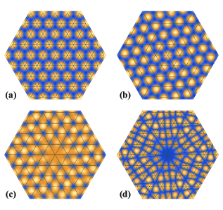
Figure 1: Density profile for the triangular moiré superlattice, as given by Eq. (2), in the cases without rotation [panel (a), $\varrho_{\theta=0}(\bm{r})$] and with a rotation of $\theta/(2\pi)=0.03$ [panel (b), $\varrho_{\theta}(\bm{r})$]. The phason excitation is illustrated by the difference in density profiles, $\mathop{}\!\delta{\varrho_{\theta}(\bm{r})}=\varrho_{\theta}(\bm{r})-\varrho_{\theta=0}(\bm{r})$, which is plotted in panel (c), and whose absolute value is plotted in panel (d). The underlying triangular lattice is a guide to the eye.

In this paper, we discuss the impact of the twist stiffness and phason damping on inevitable defects of the moiré lattice such as dislocations and disclinations. To this end, we extend the recently formulated fracton formulation of standard elasticity [19, 20, 21] to incommensurate crystals with overdamped dynamics by developing an appropriate tensor gauge field theory. The analogy to a tensor version of electromagnetism allows us to draw general conclusions about the lattice defect dynamics of TBG. The finite twist stiffness of Eq. (1) increases the degrees of freedom compared to standard elasticity theory, giving rise to a new type of defect that we call discompression. As a result, defects of the moiré lattice, which can be described in terms of fractons, are governed by an additional conservation law that dramatically affects the mobility of lattice defects. In particular, we find that in an incommensurate crystal with phason excitations, both glide and climb of dislocations are forbidden and the dynamics of defects is always sub-diffusive. This implies that dislocation networks in twisted bilayer graphene are expected to be exceptionally stable. We also show that our theory directly applies to other incommensurate systems such as planar quasicrystals.

The impact of topological lattice defects on the mechanical and electronic properties of graphene and bilayer graphene has been widely discussed [26, 27, 28]. Lattice disorder has also been recognized as a key ingredient in TBG, with experiments reporting sharp variations of the twist angle and of uniaxial heterostrain over relatively short length scales, which are manifested in local elecronic properties [29, 30]. Here, we focus on the topological defects of the emergent moiré incommensurate lattice in TBG. While its elastic properties derive from those of the coupled graphene layers, we adopt a coarse-grained low-energy description, as in Ref. [9], that does not require mapping the defects of the moiré lattice onto individual carbon atoms.

Defects of two-dimensional lattices can be efficiently captured in terms of a dual description of elasticity theory, where disclinations emerge as effective charges, dislocations as dipoles of these charges, and elastic forces between them are transmitted by gauge fields [31, 32, 33, 34, 35, 36]. This approach readily demonstrates why dislocations in commensurate lattices can glide in the direction of the Burgers vector $\bm{b}$, but not climb perpendicular to it [35]. While defects in aperiodic crystals were discussed in Ref. [37, 38, 39], their dynamics remains an open problem.

A very elegant formulation of this duality was recently achieved in Refs. [19, 20, 21, 22, 23, 24, 25]. It was recognized that the dual formulation of the usual elasticity theory is, in fact, a fracton field theory. Fracton phases describe quantum phases of matter with excitations of restricted mobility [40]. If considered in isolation, a fracton is immobile, either along certain directions or as a whole. It can only move collectively, via interactions with other degrees of freedom. Fractons were initially discussed in the context of non-ergodic quantum glass models [41] and stabilizer codes for self-correcting quantum memory [42]. More recently, it was recognized that fractons can be efficiently described in terms of tensor gauge theories [43]. The restricted mobility of fractons emerges in terms of dipole conservation laws and gives rise to anomalous, sub-diffusive hydrodynamics [44, 45, 46, 47].

II Elasticity theory of twisted bilayer graphene crystals

We start with the action of elasticity theory [33, 10], supplemented by the twist stiffness of Eq. (1). To include dissipative dynamics, we use the Schwinger-Keldysh formalism [48]:

$$\begin{aligned} S&=\frac{1}{2}\int_{\bm{x},t,t^{\prime}\in\mathcal{C}}w_{i}(\bm{x},t)D^{-1}\left(t-t^{\prime}\right)w_{i}(\bm{x},t^{\prime})\\ &-\frac{1}{2}\int_{\bm{x},t\in\mathcal{C}}\left[C_{ij,k\ell}w_{ij}(\bm{x},t)w_{k\ell}(\bm{x},t)+\kappa\vartheta_{w}^{2}(\bm{x},t)\right]\,.\end{aligned}$$ (3)

Here, $\int_{\bm{x},t\in\mathcal{C}}=\int_{\mathcal{C}}\mathop{}\!\mathrm{d}{t}\int_{V}\mathop{}\!\mathrm{d}^{2}{x}$ indicates that the time integration has to be performed on the round-trip Keldysh contour, while the spatial integration goes over the crystal volume $V$. $w_{ij}\equiv\frac{1}{2}\left(\partial_{i}w_{j}+\partial_{j}w_{i}\right)$ is the symmetric phason strain, the elastic constants $C_{ij,k\ell}$ are summarized in Ref. [9], and the bond angle variation is $\vartheta_{w}\equiv\frac{1}{2}\upepsilon_{ij}\partial_{i}w_{j}$. Damping enters through the nonlocal-in-time contribution

$$D^{-1}\left(t-t^{\prime}\right)=-\operatorname{\updelta}\left(t-t^{\prime}\right)\partial_{t^{\prime}}^{2}+\gamma\left(t-t^{\prime}\right)\,,$$ (4)

where we assume Ohmic damping $\operatorname{Im}\gamma^{R}(\omega)=\gamma_{0}\omega$ for the retarded self energy. Without damping, the equation of motion become elastic wave equations, while the dynamics becomes diffusive at large $\gamma_{0}$. For further details on the Keldysh formlism, see Appendix A.

We shall use a notation that will prove efficient in 2D. In it, we always start with lower index vectors or tensors $A_{i}$. The raising of their indices we define as a contraction with the Levi-Civita symbol:

$$A^{i}\equiv\upepsilon_{ij}A_{j}\,.$$ (5)

From $A_{i}=\left(A_{x},A_{y}\right)$ and $A^{i}\equiv\upepsilon_{ij}A_{j}$ we see that the upper index vector $A^{i}=\left(A_{y},-A_{x}\right)$ is the lower index vector rotated in the clockwise direction by $\uppi/2$. This ensures that $\bm{A}\bm{\cdot}\bm{B}=A_{i}B_{i}=A^{i}B^{i}$. On the other hand, $\left(\bm{A}\bm{\times}\bm{B}\right)_{z}=A_{i}B^{i}=-A^{i}B_{i}$ and in particular $A_{i}A^{i}=0$. The divergence and two-dimensional curl may likewise be expressed in this notation as

$$\bm{\nabla}\bm{\cdot}\bm{A} =\partial_{i}A_{i}\,,$$

$$\left(\bm{\nabla}\bm{\times}\bm{A}\right)_{z} =\partial_{i}A^{i}=-\partial^{i}A_{i}\,.$$ (6)

For single-valued functions $f$, $\partial_{i}\partial^{i}f=0$. For multivalued functions, the partial derivative do not commute at the branch cuts. The most important benefit of this notation, reminiscent of the van der Waerden spinor notation [49], is that the correspondence between elasticity and tensor electromagnetism [19, 20, 21, 22] amounts to simply raising all the indices.

II.1 Dual gauge theory

Building on the approach of Refs. [19, 20, 21], the first step in formulating a dual description is to introduce the fields $\partial_{t}w_{i}\to\pi_{i}$, $C_{ij,k\ell}w_{k\ell}\to\sigma_{ij}$, and $\kappa\vartheta_{w}\to M$ through a series of Hubbard-Stratonovich transformations. They can be associated with momentum, stress, and torque, respectively. This yields the real-time action

$$S =\frac{1}{2}\int_{\bm{x},t\in\mathcal{C}}\left[C_{ij,k\ell}^{-1}\sigma_{ij}(\bm{x},t)\sigma_{k\ell}(\bm{x},t)+\kappa^{-1}M^{2}(\bm{x},t)\right]$$

$$\quad-\frac{1}{2}\int_{\bm{x},t,t^{\prime}\in\mathcal{C}}\pi_{i}(\bm{x},t)\Gamma\left(t-t^{\prime}\right)\pi_{i}(\bm{x},t^{\prime})+S_{w}\,,$$ (7)

where the retarded version of $\Gamma$ is $\Gamma^{R}(\omega)=\omega^{2}/\left(\omega^{2}+\mathrm{i}\gamma_{0}\omega\right)$. The last term

$$S_{w}=\int_{\bm{x},t\in\mathcal{C}}\left[\pi_{i}\left(\partial_{t}w_{i}\right)-\sigma_{ij}w_{ij}-M\vartheta_{w}\right]$$ (8)

still contains the original phason field.

The next step is to decompose $w_{i}=\tilde{w}_{i}+w_{i}^{(s)}$ into a smooth part $\tilde{w}_{i}$ and a singular part $w_{i}^{(s)}$ due to topological defects. After integrating out the smooth part, we obtain the constraint

$$\partial_{t}\pi_{j}=\partial_{i}\Sigma_{ij}\,,$$ (9)

which resembles Newton’s second law with a non-symmetric stress

$$\Sigma_{ij}=\sigma_{ij}+\frac{1}{2}\upepsilon_{ij}M\,,$$ (10)

consisting of the symmetric stress tensor $\sigma_{ij}$ and the torque $M$. Whereas $\sigma_{ij}$ also appears in ordinary crystals, the torque only arises due to the finite twist stiffness.

The last step is to introduce (tensorial) gauge potentials that enforce the constraint (9):

$$\begin{aligned} \Sigma_{ij}&=-\partial_{t}A_{ij}-\partial^{i}\phi_{j}\,,\\ \pi_{j}&=-\partial_{i}A_{ij}\,.\end{aligned}$$ (11)

These gauge potentials are invariant under the gauge transformations

$$\begin{aligned} A_{ij}&\mapsto A_{ij}+\partial^{i}\Lambda_{j}\,,\\ \phi_{j}&\mapsto\phi_{j}-\partial_{t}\Lambda_{j}\,.\end{aligned}$$ (12)

The stress-strain coupling Eq. (8) now takes the familiar form of a charge/current-potential coupling:

$$S_{w}=\int_{\bm{x},t\in\mathcal{C}}\left(A_{ij}J_{ij}-\phi_{j}Q_{j}\right)\,.$$ (13)

Due to the tensorial nature of the gauge fields, the charge density

$$Q_{j}=\partial^{i}\partial_{i}w_{j}^{(s)}$$ (14)

is a vector and the corresponding current density,

$$J_{ij}=\left(\partial_{i}\partial_{t}-\partial_{t}\partial_{i}\right)w_{j}^{(s)}\,,$$ (15)

a tensor. Demanding the invariance of (13) under the gauge transformations yields the continuity equation:

$$\partial_{t}Q_{j}+\partial^{i}J_{ij}=0\,.$$ (16)

II.2 Electromagnetic analogy

Let us develop, in analogy to Ref. [19, 20, 21, 22] for standard elasticity, a physical illuminating electromagnetic analogy of the conserved vector charge $Q_{j}$. Consider a single charge

$$Q_{j}(\bm{x},t)=q_{j}\operatorname{\updelta}\left(\bm{x}-\bm{r}(t)\right)$$ (17)

at position $\bm{r}(t)$ that moves with velocity $\bm{v}(t)=\dot{\bm{r}}(t)$. Eq. (16) is then fulfilled by

$$J_{ij}(\bm{x},t)=v^{i}q_{j}\operatorname{\updelta}\left(\bm{x}-\bm{r}(t)\right)\,.$$ (18)

Inserting this into the action (13) yields the Lorentz force

$$F_{i}=\mathop{}\!\delta{S_{w}}/\mathop{}\!\delta{r_{i}}=-\left(\Sigma^{i}_{\leavevmode\nobreak\ j}+v^{i}\pi_{j}\right)q_{j}\,.$$ (19)

The problem behaves like the electrodynamics of non-symmetric tensor electric fields $\Sigma^{i}_{\leavevmode\nobreak\ j}$ and vector magnetic fields $\pi_{i}$. This analogy also helps us understand why the overdamped dynamics of the phasons does not spoil the entire gauge description. The dissipative propagator $\Gamma(t-t^{\prime})$ for $\pi_{i}(t)$ in Eq. (7) translates, in standard electromagnetism, to a frequency-dependent magnetic permeability $\Gamma(\omega)$, which clearly does not violate the gauge description of electromagnetism.

Besides the effects of dissipation, a crucial new aspect of the incommensurate moiré lattice elasticity is the vector continuity equation (16) that can be rephrased in terms of two conserved scalar densities:

$$\begin{aligned} \rho^{(\ell)}&=\partial_{j}Q_{j}\,,\\ \rho^{(t)}&=\partial^{j}Q_{j}\,,\end{aligned}$$ (20)

with continuity equations

$$\begin{aligned} \partial_{t}\rho^{(\ell)}+\partial_{j}\partial^{i}J_{ij}&=0\,,\\ \partial_{t}\rho^{(t)}+\partial^{j}\partial^{i}J_{ij}&=0\,.\end{aligned}$$ (21)

The transverse density $\rho^{(t)}$ also appears in standard elasticity, where it was identified as the density of disclinations, with $Q_{i}$ denoting the Burgers vector density [34, 19]. The longitudinal density $\rho^{(\ell)}$ is the new conserved charge present only in incommensurate crystals.

II.3 Interpretation of the charges

The charges of the elastic gauge theory are topological lattice defects that make the displacement field $w_{i}$ multivalued [36]. We can write the singular part of a dislocation displacement field as

$$\bm{w}^{(s,Q)}(\bm{x})=\frac{\operatorname{Im}\operatorname{Log}(z)}{2\uppi}\,\bm{b}\,,$$ (22)

where $z=x_{1}+\mathrm{i}x_{2}$, $\operatorname{Log}(z)$ is the principal branch of the logarithm with a branch cut along the negative $x_{1}$ axis, and $\bm{b}=b_{1}\bm{\hat{e}}_{1}+b_{2}\bm{\hat{e}}_{2}$ is the Burgers vector. At the origin the partial derivatives do not commute, yielding $Q_{j}(\bm{x})=b_{j}\operatorname{\updelta}(\bm{x})$, which confirms that the vector charge is the Burgers vector density.

Next, we construct a disclination from a Dirac string of dislocations. By integrating $\int_{-\infty}^{0}\mathop{}\!\mathrm{d}{x_{1}^{\prime}}\,\bm{w}^{(s,Q)}(x_{1}-x_{1}^{\prime},x_{2})$, ignoring all except the singular parts, and setting $b_{1}=0$ and $b_{2}\neq 0$, we obtain

$$\bm{w}^{(s,t)}(\bm{x})=-b_{2}\frac{\operatorname{Im}\left[z\operatorname{Log}(z)\right]}{2\uppi}\,\bm{\hat{e}}_{2}\,,$$ (23)

with $Q_{j}=b_{2}\updelta_{2j}\Theta(-x_{1})\operatorname{\updelta}(x_{2})$, $\rho^{(\ell)}=b_{2}\Theta(-x_{1})\operatorname{\updelta}^{\prime}(x_{2})$, and $\rho^{(t)}=b_{2}\operatorname{\updelta}(\bm{x})$. This confirms that $\rho^{(t)}$ is the density of disclinations. In addition, the result for $\rho^{(l)}$ implies that a disclination also corresponds to a Dirac string along the negative $x_{1}$-axis made of dipoles ($\sim\operatorname{\updelta}^{\prime}(x_{2})$) of the longitudinal charge.

Similarly, we may consider a Dirac string of dislocations whose Burgers vectors point along the branch cut, instead of perpendicular to it ($b_{1}\neq 0$ and $b_{2}=0$),

$$\bm{w}^{(s,\ell)}(\bm{x})=-b_{1}\frac{\operatorname{Im}\left[z\operatorname{Log}(z)\right]}{2\uppi}\,\bm{\hat{e}}_{1}\,.$$ (24)

The charges are $Q_{j}=b_{1}\updelta_{1j}\Theta(-x_{1})\operatorname{\updelta}(x_{2})$, $\rho^{(\ell)}=-b_{1}\operatorname{\updelta}(\bm{x})$, and $\rho^{(t)}=b_{1}\Theta(-x_{1})\operatorname{\updelta}^{\prime}(x_{2})$. Since $\bm{w}^{(s,\ell)}$ points parallel to the Dirac string, and its jump in value is proportional to the distance from the origin, it represents an abrupt change in the strain. We shall thus call this defect a discompression. Below Eq. (23) we showed that a disclination is equivalent to a Dirac string of discompression dipoles. The result for $\rho^{(t)}$ implies, in turn, that a discompression equals a Dirac string of disclination dipoles. These “fusion rules” for the various defects are sketched in the lower part of Fig. 2.

In Fig. 2, we show these defects for a triangular lattice. Disclinations and discompressions are energetically very expensive as both come along with macroscopic regions of compression or bond-angle mismatch. More formally, both are forbidden as single charges by an appropriate generalization of Weingarten’s theorem [36]. Hence, a moiré lattice is charge neutral with regards to $\rho^{(t,\ell)}$, while their dipoles and higher moments remain perfectly valid excitations. Fig. 2(c) illustrates the known fact that a dislocation corresponds to a dipole of disclinations (panels (a) and (b)) with dipole moment perpendicular to the Burgers vector $\bm{b}$. Our analysis shows that a dislocation [Fig. 2(f)] can also emerge from two discompressions of opposite charge (panels (d) and (e)). The dipole moment is now oriented along the Burgers vector. Single discompressions of Fig. 2(d) and (e) can be generated in terms of a Volterra process where we cut along the negative $x_{1}$-axis and displace matter above and below the cut in opposite directions parallel to the cut, before glueing back together. This is distinct from disclinations of Fig. 2(a) and (b) where the displacement is perpendicular to the cut and opens a wedge.

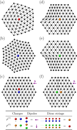
Figure 2: Various defects for a triangular lattice and the relations between them. (a) Positive disclination ($b_{2}=2/\sqrt{3}$). (b) Negative disclination ($b_{2}=-2/\sqrt{3}$). (c) Dislocation as a dipole of disclinations. (d) Positive discompression ($b_{1}=1/2$). (e) Negative discompression ($b_{1}=-1/2$). (f) Dislocation as a dipole of discompressions. The table summarizes the fusion rules that explain how to represent charges in terms of Dirac strings of dipoles of other charges.

II.4 Consequences of the continuity equations

Eq. (16) implies the conservation of the total Burgers vector. Let us analyze this vector conservation law in terms of the continuity equations (21) of the scalar densities that both contain two spatial derivatives. This implies, in addition to the conservation of the total disclination and discompression charges, that both of their total dipole moments are conserved as well:

$$\frac{\mathop{}\!\mathrm{d}{}}{\mathop{}\!\mathrm{d}{t}}\int\mathop{}\!\mathrm{d}^{2}{x}\ x_{k}\,\rho^{(\ell,t)}=0\,.$$ (25)

Both charges are therefore immobile fractons. Only correlated movements at fixed dipole density are allowed.

II.5 Energetics and equations of motion

Thus far we analyzed conservation laws that follow from the gauge invariance of the dual theory. To understand the actual dynamics of defects requires, however, an analysis of the energetics of vector charges. To this end we determine the equations of motion of the gauge fields that mediate the stresses. The Euler-Lagrange equation of $A_{ij}$ is:

$$\partial_{t}\tilde{\Sigma}_{ij}(t)=\int\mathop{}\!\mathrm{d}{t^{\prime}}\,\Gamma^{R}\left(t-t^{\prime}\right)\partial_{i}\pi_{j}(t^{\prime})-J_{ij}(t)\,,$$ (26)

with $\tilde{\Sigma}_{ij}=C_{ij,k\ell}^{-1}\sigma_{k\ell}+\upepsilon_{ij}\kappa^{-1}M$. It is the analog of Ampere’s law in electrodynamics. The analog of Gauss’s law $\partial^{i}\tilde{\Sigma}_{ij}=Q_{j}$ follows from the variation of the potential $\phi_{j}$ and demonstrates that $Q_{j}$ is indeed the source of stress.

We can use Ampere’s law to determine the dynamics of the quadrupolar moments. To achieve this, we first contract the Euler-Lagrange equation (26) with $\updelta_{ij}$ and $\upepsilon_{ij}$. This gives

$$\partial_{t}C_{ii,k\ell}^{-1}\sigma_{k\ell} =\partial_{i}(\Gamma^{R}\pi_{i})-J_{ii}\,,$$ (27)

$$\frac{2}{\kappa}\partial_{t}M =\partial_{i}(\Gamma^{R}\pi^{i})-J^{\leavevmode\nobreak\ i}_{i}\,,$$ (28)

where

$$\left(\Gamma^{R}\pi_{j}\right)(\bm{x},t)=\int\mathop{}\!\mathrm{d}{t^{\prime}}\,\Gamma^{R}\left(t-t^{\prime}\right)\pi_{j}(\bm{x},t^{\prime})\,.$$ (29)

Now we use the conservation laws (21), partially integrate the quadrupolar moments twice, and then use the equations of motion. This yields

$$\frac{\mathop{}\!\mathrm{d}{}}{\mathop{}\!\mathrm{d}{t}}\int_{V}\left\lvert{\bm{x}}\right\rvert^{2}\rho^{(t)}\leavevmode\nobreak\ \overset{\mathclap{\eqref{continuity_div_p}}}{=}\leavevmode\nobreak\ -\int_{V}x_{k}x_{k}\partial^{j}\partial^{i}J_{ij}$$ (30)

$$=-2\int_{V}J_{ii}+\int_{V}\partial_{j}\left(2x_{i}J^{ji}-\left\lvert{\bm{x}}\right\rvert^{2}\partial_{i}J^{ij}\right)$$

$$\overset{\mathclap{\eqref{contr_delta}}}{=}\leavevmode\nobreak\ 2\int_{V}\partial_{t}C_{ii,k\ell}^{-1}\sigma_{k\ell}$$

$$+\int_{V}\partial_{j}\left(2x_{i}J^{ji}-\left\lvert{\bm{x}}\right\rvert^{2}\partial_{i}J^{ij}-2\Gamma^{R}\pi_{j}\right)$$

and

$$\frac{\mathop{}\!\mathrm{d}{}}{\mathop{}\!\mathrm{d}{t}}\int_{V}\left\lvert{\bm{x}}\right\rvert^{2}\rho^{(\ell)}\leavevmode\nobreak\ \overset{\mathclap{\eqref{continuity_div_p}}}{=}\leavevmode\nobreak\ -\int_{V}x_{k}x_{k}\partial_{j}\partial^{i}J_{ij}$$ (31)

$$=-2\int_{V}J^{\leavevmode\nobreak\ i}_{i}+\int_{V}\partial_{j}\left(\left\lvert{\bm{x}}\right\rvert^{2}\partial_{i}J^{i}_{\leavevmode\nobreak\ \,j}-2x_{i}J^{j}_{\leavevmode\nobreak\ \,i}\right)$$

$$\overset{\mathclap{\eqref{contr_epsilon}}}{=}\leavevmode\nobreak\ \frac{4}{\kappa}\int_{V}\partial_{t}M$$

$$+\int_{V}\partial_{j}\left(\left\lvert{\bm{x}}\right\rvert^{2}\partial_{i}J^{i}_{\leavevmode\nobreak\ \,j}-2x_{i}J^{j}_{\leavevmode\nobreak\ \,i}-2\Gamma^{R}\pi^{j}\right)\,.$$

Finally, we rewrite the sources by exploiting the Euler-Lagrange equations of the action (7), $C_{ij,k\ell}^{-1}\sigma_{k\ell}=w_{ij}$ and $M=\kappa\vartheta_{w}$, and thus obtain

$$\frac{\mathop{}\!\mathrm{d}{}}{\mathop{}\!\mathrm{d}{t}}\int\mathop{}\!\mathrm{d}^{2}{x}\,\left\lvert{\bm{x}}\right\rvert^{2}\rho^{(\ell,t)}=\frac{\mathop{}\!\mathrm{d}{}}{\mathop{}\!\mathrm{d}{t}}S^{(\ell,t)}\,.$$ (32)

The source terms for disclination quadrupoles is

$$S^{(t)}=2\int\mathop{}\!\mathrm{d}^{2}{x}\,\partial_{i}w_{i}$$ (33)

and corresponds to a costly volume change of the system. In turn,

$$S^{(\ell)}=4\int\mathop{}\!\mathrm{d}^{2}{x}\,\vartheta_{w}$$ (34)

for discompression quadrupoles corresponds to a global twist. These quadrupoles can easily be interpreted if one considers an isolated dislocation $Q_{j}(\bm{x})=b_{j}\operatorname{\updelta}\left(\bm{x}-\bm{r}(t)\right)$ whose $\int\mathop{}\!\mathrm{d}^{2}{x}\,\left\lvert{\bm{x}}\right\rvert^{2}\rho^{(t)}=2b^{j}r_{j}(t)$ and $\int\mathop{}\!\mathrm{d}^{2}{x}\,\left\lvert{\bm{x}}\right\rvert^{2}\rho^{(\ell)}=-2b_{j}r_{j}(t)$. Thus the quadrupolar moments are the components of the dislocation position parallel and perpendicular to the Burgers vector. Eq. (32) was obtained up to boundary terms. The boundary terms vanish or, more physically, cannot be changed by local operations that act in the bulk of the medium. Thus (32) expresses how in the bulk the sources of changing quadrupolar moments are the energetically costly compression and disorientation of the crystal.

In our analysis we freely used expressions that are valid only on-shell, the various conservation laws (16, 21, 25, 32), equations of motion (60, 26, $C_{ij,k\ell}^{-1}\sigma_{k\ell}=\partial_{i}w_{j}$, $M=\kappa\vartheta_{w}$), expressions for the sources $S^{(t)}$ and $S^{(\ell)}$, etc., can all be formulated as rigorous statements that apply to the respective path-integral averages. This is proved by using the Schwinger-Dyson equations.

From Eq. (32) we may therefore conclude that a climb, i.e. the motion perpendicular to $b_{j}$ of a dislocation, is accompanied by an energetically costly change in the volume of the crystal. In addition, a glide, i.e. the motion parallel to $b_{j}$ of a dislocation, is accompanied by an energetically costly change of the orientation of the crystal. While the first result holds in any crystal, the second is due to the non-zero twist stiffness of incommensurate ones. In its presence the motion of dislocations is forbidden entirely instead of just being restricted to one direction.

II.6 Sub-diffusive hydrodynamics

Thus far we have analyzed the motion of isolated dipoles and quadrupoles. The situation becomes more complicated for higher-order multipoles. However, using the hydrodynamic description of fractons [44, 45, 46, 47] one readily finds that there cannot be a Fick’s law where gradients of the vector charges yield currents (i.e. $J_{ij}\propto\partial_{i}Q_{j}$ or $\propto\partial^{i}Q_{j}$), leading to ordinary diffusion of all charges. If this were true, the mere existence of scalar charges would induce a current $J_{ii}\sim\rho^{(\ell,t)}$, which is not allowed. Expanding in gradients, the leading symmetry-allowed term connects $J_{ij}$ with a third spatial derivative of $Q_{j}$. This gives rise to a coupled dynamics of the two scalar densities that form two sub-diffusive modes with dispersions $\omega=\mathrm{i}B_{\pm}k^{4}$.

III Generalization to generic planar quasicrystals and incommensurate crystals

Finally, we demonstrate that our results are not restricted to TBG and apply directly to planar quasicrystals and incommensurate crystals with two length scales. To this end we relate the elastic gauge theory with twisting term considered in the main text to the elasticity theory of two-dimensional quasicrystals. In these systems, the low-energy elastic variables are doubled compared to periodic crystals [11, 12, 13]. In addition to the phonons $\bm{u}$, there are phasons $\bm{w}$ that can be shown to have a twist stiffness like in Eq. (1). The defects of the system are characterized by two Burgers vectors $\bm{b}_{u}=\oint\mathop{}\!\mathrm{d}{\bm{u}}$ and $\bm{b}_{w}=\oint\mathop{}\!\mathrm{d}{\bm{w}}$ [12]. Our results imply that pure displacement dislocations can glide, whereas those that involve $\bm{b}_{w}$ cannot. This remains true even in the presence of phonon-phason coupling.

A symmetry analysis of the problem yields the following result for the elastic energy [11, 12, 13]:

$$\mathcal{E}_{\text{el}}=\frac{1}{2}C_{ij,k\ell}u_{ij}u_{k\ell}+R_{ij,k\ell}u_{ij}w_{k\ell}+\frac{1}{2}K_{ij,k\ell}w_{ij}w_{k\ell}\,,$$ (35)

where $u_{ij}=\frac{1}{2}\left(\partial_{i}u_{j}+\partial_{j}u_{i}\right)$ is the usual symmetric strain tensor describing phonons and $w_{ij}=\partial_{i}w_{j}$ is the non-symmetric phason tensor.

For the moment, let us focus on the case of a twelvefold symmetric planar quasicrystals that has the special property of no phonon-phason mixing, i.e., $R_{ij,k\ell}=0$ [13]. Because of the high rotational symmetry, the elastic constants $C_{ij,k\ell}$ have the same form as those of isotropic media:

$$C_{ij,k\ell}=\lambda\,\updelta_{ij}\updelta_{k\ell}+\mu\,\left(\updelta_{ik}\updelta_{j\ell}+\updelta_{i\ell}\updelta_{jk}\right)\,.$$ (36)

On the other hand,

$$K_{ij,k\ell}=K_{1}\updelta_{ik}\updelta_{j\ell}+K_{2}\left(\updelta_{ij}\updelta_{k\ell}-\updelta_{i\ell}\updelta_{jk}\right)+\tilde{K}_{3}\upepsilon^{S}_{ij}\upepsilon^{S}_{k\ell}\,,$$ (37)

where $\upepsilon^{S}_{11}=\upepsilon^{S}_{22}=0$ and $\upepsilon^{S}_{12}=\upepsilon^{S}_{21}=1$. We note that $K_{ij,k\ell}$ satisfies only the major index symmetry $K_{ij,k\ell}=K_{k\ell,ij}$, but not the minor ones $K_{ij,k\ell}\neq K_{ji,k\ell}$ and $K_{ij,k\ell}\neq K_{ij,\ell k}$.

To make contact with our system (3), we merely have to recognize that $K_{ij,k\ell}$ can be rewritten as

$$K_{ij,k\ell}=\tilde{C}_{ij,k\ell}+\frac{\kappa}{4}\upepsilon_{ij}\upepsilon_{k\ell}\,,$$ (38)

where

$$\tilde{C}_{ij,k\ell}=\tilde{\lambda}\,\updelta_{ij}\updelta_{k\ell}+\tilde{\mu}\,\left(\updelta_{ik}\updelta_{j\ell}+\updelta_{i\ell}\updelta_{jk}\right)+\tilde{K}_{3}\upepsilon^{S}_{ij}\upepsilon^{S}_{k\ell}$$ (39)

is the minor-index-symmetric part that satisfies $\tilde{C}_{ij,k\ell}=\tilde{C}_{ji,k\ell}=\tilde{C}_{ij,\ell k}$ and has $\tilde{\lambda}=K_{2}$ and $\tilde{\mu}=\frac{1}{2}\left(K_{1}-K_{2}\right)$. The minor-index-antisymmetric part plays the role of a twisting term with stiffness

$$\kappa=2\left(K_{1}+K_{2}\right)\,.$$ (40)

Thus the phonon displacement field $u_{i}$ behaves like in the elasticity theory of a conventional crystal, while the phason $w_{i}$ is governed by an elastic energy identical to the one of twisted bilayer graphene, given in Eq. (1) or (3). Hence all our conclusions about the mobility of defects of the phason modes carry over.

The situation is more complicated for quasicrystals with fivefold or eightfold symmetry. In these cases, $C_{ij,k\ell}$ is still isotropic, as in (36), and $K_{ij,k\ell}$ still has the form (37), although with $\tilde{K}_{3}=0$ in the case of fivefold symmetry, and can therefore be decomposed according to (38). Most significantly, a phonon-phason coupling of the form

$$R_{ij,k\ell}=R\left(\updelta_{i1}-\updelta_{i2}\right)\left[\updelta_{ij}\updelta_{k\ell}+\updelta_{ik}\updelta_{j\ell}-\updelta_{i\ell}\updelta_{jk}\right]$$ (41)

is allowed. Consequently, one has to redo the whole gauge formulation.

The end results, however, turn out to be insensitive to phonon-phason coupling. Specifically, for the phonon field one finds the usual results [19, 20, 21]:

$$\partial_{t}\rho^{(t)}_{u}+\partial^{j}\partial^{i}J_{uij}^{S} =0\,,$$ (42)

$$\frac{\mathop{}\!\mathrm{d}{}}{\mathop{}\!\mathrm{d}{t}}\int\mathop{}\!\mathrm{d}^{2}{x}\ x_{k}\,\rho^{(t)}_{u} =0\,,$$ (43)

$$\frac{\mathop{}\!\mathrm{d}{}}{\mathop{}\!\mathrm{d}{t}}\int\mathop{}\!\mathrm{d}^{2}{x}\,\left\lvert{\bm{x}}\right\rvert^{2}\rho^{(t)}_{u} =\frac{\mathop{}\!\mathrm{d}{}}{\mathop{}\!\mathrm{d}{t}}S^{(t)}_{u}\,,$$ (44)

where $Q_{uj}=\partial^{i}\partial_{i}u_{j}^{(s)}$, $J_{uij}=\left(\partial_{i}\partial_{t}-\partial_{t}\partial_{i}\right)u_{j}^{(s)}$, $\rho^{(t)}_{u}=\partial^{j}Q_{uj}$, $J_{uij}^{S}=\frac{1}{2}\left(J_{uij}+J_{uji}\right)$, and $S^{(t)}_{u}=2\int\mathop{}\!\mathrm{d}^{2}{x}\,\partial_{i}u_{i}$. For the phason fields one similarly finds that (16), (21), (25), and (32) continue to hold, but with the appropriate $Q_{wj}=\partial^{i}\partial_{i}w_{j}^{(s)}$, $J_{wij}=\left(\partial_{i}\partial_{t}-\partial_{t}\partial_{i}\right)w_{j}^{(s)}$, $\rho^{(\ell)}_{w}=\partial_{j}Q_{wj}$, $\rho^{(t)}_{w}=\partial^{j}Q_{wj}$, $S^{(t)}_{w}=2\int\mathop{}\!\mathrm{d}^{2}{x}\,\partial_{i}w_{i}$, and $S^{(\ell)}_{w}=4\int\mathop{}\!\mathrm{d}^{2}{x}\,\vartheta_{w}$. Therefore, the glide of defects that have a finite phason Burgers vectors $\bm{b}_{w}=\oint\mathop{}\!\mathrm{d}{\bm{w}}$ is suppressed, and the parameter that controls the supression is the effective twisting stiffness (40).

Details of the phonon-phason coupled gauge theory: It is convenient to introduce an additional index $\mu,\nu\in\{u,w\}$ that differentiates the phonon and phason displacement fields. That way, $u_{ui}=u_{i}$, $u_{wi}=w_{i}$, $u_{uij}=u_{ij}$, $u_{wij}=w_{ij}$, and

$$C_{uij,uk\ell}=C_{ij,k\ell}\,,\quad C_{wij,wk\ell}=K_{ij,k\ell}\,,$$ (45)

$$C_{uij,wk\ell}=C_{wk\ell,uij}=R_{ij,k\ell}\,.$$ (46)

The appropriate generalization of the action (3) we may now write as

$$\begin{aligned} S&=\frac{1}{2}\int_{\bm{x},t,t^{\prime}\in\mathcal{C}}u_{\mu i}(t)D^{-1}_{\mu}\left(t-t^{\prime}\right)u_{\mu i}(t^{\prime})\\ &\qquad-\frac{1}{2}\int_{\bm{x},t\in\mathcal{C}}C_{\mu ij,\nu k\ell}u_{\mu ij}u_{\nu k\ell}\,.\end{aligned}$$ (47)

Next, we introduce the Hubbard-Stratonovich fields $\partial_{t}u_{\mu i}\to\pi_{\mu i}$ and $C_{\mu ij,\nu k\ell}u_{\nu k\ell}\to\Sigma_{\mu ij}$, integrate out the regular parts of $u_{\mu i}$, and then enforce the constraints $\partial_{t}\pi_{\mu j}=\partial_{i}\Sigma_{\mu ij}$ through gauge potentials:

$$\begin{aligned} \Sigma_{uij}&=-\partial_{t}A_{uij}^{S}-\partial^{i}\partial^{j}\phi_{u}\,,\\ \pi_{uj}&=-\partial_{i}A_{uij}^{S}\,,\end{aligned}$$ (48)

$$\begin{aligned} \Sigma_{wij}&=-\partial_{t}A_{wij}-\partial^{i}\phi_{wj}\,,\\ \pi_{wj}&=-\partial_{i}A_{wij}\,,\end{aligned}$$ (49)

where $A_{uij}^{S}=A_{uji}^{S}$ is symmetric. This yields the action

$$\begin{aligned} S&=-\frac{1}{2}\int_{\bm{x},t,t^{\prime}\in\mathcal{C}}\pi_{\mu i}(t)\Gamma_{\mu}\left(t-t^{\prime}\right)\pi_{\mu i}(t^{\prime})\\ &\qquad+\frac{1}{2}\int_{\bm{x},t\in\mathcal{C}}C_{\mu ij,\nu k\ell}^{-1}\Sigma_{\mu ij}\Sigma_{\nu k\ell}+S_{uw}\,,\end{aligned}$$ (50)

where $\Gamma_{\mu}\left(t-t^{\prime}\right)=\overleftarrow{\partial_{t}}D_{\mu}\left(t-t^{\prime}\right)\overrightarrow{\partial_{t^{\prime}}}$ and

$$\begin{aligned} S_{uw}=\int_{\bm{x},t\in\mathcal{C}}\big{[}&A_{uij}^{S}J_{uij}^{S}+\phi_{u}\rho^{(t)}_{u}\\ &+A_{vij}J_{vij}-\phi_{vj}Q_{vj}\big{]}\,,\end{aligned}$$ (51)

with the previously defined charges and current densities.

In this action we see why the phonon-phason coupling does not affect the argument leading to the quadrupolar conservation laws. On the one hand, the charge conservation laws are a consequence of the local gauge symmetry and from the form of the source term (51) we immediately see that they are unaffected by $C_{\mu ij,\nu k\ell}^{-1}$ or $R_{ij,k\ell}$. On the other hand, let us take a look at the Euler-Lagrange equations of $A_{\mu ij}$ that allowed for an additional partial integration in (30) and (31):

$$\partial_{t}\tilde{\Sigma}_{\mu ij}(t)=\int\mathop{}\!\mathrm{d}{t^{\prime}}\,\Gamma^{R}_{\mu}\left(t-t^{\prime}\right)\partial_{i}\pi_{\mu j}(t^{\prime})-J_{\mu ij}(t)\,.$$ (52)

Once one expresses $\tilde{\Sigma}_{\mu ij}=C_{\mu ij,\nu k\ell}^{-1}\Sigma_{\nu k\ell}$ in terms of the original fields $u_{\mu ij}$, one finds that $\tilde{\Sigma}_{\mu ij}=u_{\mu ij}$ according to the Euler-Lagrange equations of $\Sigma_{\mu ij}$. Thus $C_{\mu ij,\nu k\ell}$ again drop out of the argument. Therefore, $C_{\mu ij,\nu k\ell}$ formally influence the argument only through the symmetry properties that they entail for $\Sigma_{\mu ij}$. Physically, however, $C_{\mu ij,\nu k\ell}$ also set the energy scales of glide and climb suppressions.

IV Conclusions

The dual formulation of elasticity theory that exploits the concept of fractons allows for rather general insights into the mobility of dissipative incommensurate crystals, such as twisted bilayer graphene. In particular, we find that these systems have, in distinction to usual crystals, completely immobile dislocations in the low defect density limit that become sub-diffusive in the high-density limit. Hence, while the electronic properties of graphene can, to a very good approximation, be treated using concepts of periodic crystals [5, 6, 7, 8], the incommensurate nature of the material is much more visible in its mechanical properties. In order to estimate whether the effects discussed here are quantitatively relevant, we follow [9]. Here, $\kappa$ is shown to be of the order of $10\text{eV}/\text{nm}^{2}\sin\left(\Theta/2\right)$. For twist angles $\Theta\sim 1^{\circ}$ this yields $\kappa\sim 0.1\text{eV}/\text{nm}^{2}$. Hence, on the length scale of the moiré crystal $\sim 10\text{nm}$, this stiffness is clearly relevant in a wide temperature regime.

Our results are not unique to twisted bilayer graphene. As we demonstrate in section III, they can be generalized to generic planar quasicrystals and incommensurate crystals. The lack of mobility of defects stabilizes networks of defects, such as the soliton network discussed in Ref. [9]. Another implication is that these incommensurate systems should mechanically be rather brittle.

The power of the formalism that led to the results of this work is drawn primarily from the deep intuition that follows from the analogy to electromagnetism, including multipole expansions or the electromagnetism of dissipative media. An interesting open question is how the properties of these defects, and particularly the discompressions, impact the global mechanical properties of TBG, as well as its local electronic spectrum, where stable defect configurations on the electronic spectrum are expected to lead to localized bound state formation. For isolated disclinations and discompressions one might even expect topologically protected bound states in the electronic spectrum [50].

Note added: After this work was completed, we became aware of interesting related works concerned with a fracton description [51] and topologically protected defect motion [52] of quasicrystals.

Appendix A Schwinger-Keldysh formulation of the elasticity theory

In order to include damping of fractons, we perform the analysis on the Keldysh contour [48]. We consider the generating functional:

$$W\left[h_{i}\right]=\int\mathcal{D}w\,\mathrm{e}^{\mathrm{i}S\left[w\right]-\mathrm{i}\int_{\mathcal{C}}h_{i}\left(t\right)w_{i}\left(t\right)}\,.$$ (53)

Here, $\int_{x,t\in\mathcal{C}}\cdots=\int_{\mathcal{C}}\mathop{}\!\mathrm{d}{t}\int_{V}\mathop{}\!\mathrm{d}^{2}{x}\cdots$ indicates that the time integration has to be performed on the round-trip Keldysh contour, while the spatial integration goes over the volume $V$. The action of the problem is given in Eq. (3), where the damping term enters through the nonlocal-in-time contribution

$$D^{-1}\left(t-t^{\prime}\right)=-\operatorname{\updelta}\left(t-t^{\prime}\right)\partial_{t^{\prime}}^{2}+\gamma\left(t-t^{\prime}\right)\,,$$ (54)

with friction self energy term $\gamma\left(t\right)$. Let $w_{i}^{+}\left(t\right)$ and $w_{i}^{-}\left(t\right)$ refer to the phason modes on the upper and lower contour, respectively. Transforming the Keldysh degrees of freedom to quantum and classical fields

$$w_{i}^{c,q}\left(t\right)=\frac{1}{\sqrt{2}}\left(w_{i}^{+}\left(t\right)\pm w_{i}^{-}\left(t\right)\right)\,,$$ (55)

the self energy as function of frequency takes the form

$$\gamma\left(\omega\right)=\begin{pmatrix}0&\gamma^{R}\left(\omega\right)\\ \gamma^{A}\left(\omega\right)&\gamma^{K}\left(\omega\right)\end{pmatrix}\,.$$ (56)

We assume Ohmic damping

$$\operatorname{Im}\gamma^{R}\left(\omega\right)=\gamma_{0}\omega\mathrm{e}^{-\left\lvert{\omega}\right\rvert/\omega_{c}}$$ (57)

with upper cutoff $\omega_{c}$. The real part of $\gamma^{R}\left(\omega\right)$ is determined via a Kramers-Kronig transformation, where constant terms $\gamma^{R}\left(0\right)$ have to be subtracted. In addition,

$$\gamma^{K}\left(\omega\right)=-2\coth\left(\frac{\omega}{2T}\right)\operatorname{Im}\gamma^{R}\left(\omega\right)$$ (58)

follows from the fluctuation-dissipation theorem. Hence, the retarded Fourier transform is at low energies given by

$$D^{R}\left(\omega\right)=\frac{1}{\omega^{2}+\mathrm{i}\gamma_{0}\omega}\,.$$ (59)

At low frequencies, the damping term is the dominant one. The equations of motion for the displacement fields $w_{i}$ are

$$\begin{aligned} \frac{\partial^{2}w_{j}}{\partial t^{2}}&=\int\mathop{}\!\mathrm{d}{t^{\prime}}\,\gamma^{R}\left(t-t^{\prime}\right)w_{j}(t^{\prime})\\ &\qquad+\partial_{i}\left[C_{ij,k\ell}w_{k\ell}+\tfrac{1}{2}\upepsilon_{ij}\kappa\vartheta_{w}\right]\,.\end{aligned}$$ (60)

For strong damping and long times $\int\mathop{}\!\mathrm{d}{t^{\prime}}\,\gamma^{R}\left(t-t^{\prime}\right)\to-\gamma_{0}\partial_{t}$, and the dynamics is diffusive. When we perform the Hubbard-Stratonovich transformations, we obtain Eq. (7) with

$$\Gamma\left(t-t^{\prime}\right)=\overleftarrow{\partial}_{t}D\left(t-t^{\prime}\right)\overrightarrow{\partial}_{t^{\prime}}\,.$$ (61)

The retarded version of $\Gamma$ becomes

$$\Gamma^{R}\left(\omega\right)=\frac{\omega^{2}}{\omega^{2}+\mathrm{i}\gamma_{0}\omega}\,.$$ (62)

In the limit $\gamma_{0}\to 0$, $\Gamma^{R}\left(\omega\right)\to 1$.