Topologically-driven three-spin chiral exchange interactions
treated from first principles

Abstract

The mechanism behind the three-spin chiral interaction (TCI) included in the extended Heisenberg Hamiltonian and represented by an expression worked out recently (Phys. Rev. B, 101, 174401 (2020)) is discussed. It is stressed that this approach provides a unique set of the multispin exchange parameters which are independent of each other either due to their different order of perturbation or due to different symmetry. This ensures in particular the specific properties of the TCI that were demonstrated previously via fully relativistic first principles calculations, and that result from the common influence of several issues not explicitly seen from the expression for the TCI parameters. Therefore, an interpretation of the TCI is suggested, showing explicitly its dependence on the relativistic spin-orbit coupling and on the topological orbital susceptibility (TOS). This is based on an expression for the TOS that is worked out on the same footing as the expression for the TCI. Using first-principles calculations we demonstrate in addition numerically the common topological properties of the TCI and TOS. To demonstrate the role of the relativistic spin-orbit coupling (SOC) for the TCI, a so-called ’topological’ spin susceptibility (TSS) is introduced. This quantity characterizes the SOC induced spin magnetic moment on the atom in the presence of non-collinear magnetic structure, giving a connection between the TOS and TCI. Numerical results again support our conclusions.

I Introduction

I.1 Interatomic exchange interaction parameters and their calculation

The classical Heisenberg model for interacting spins is a powerful platform used for the investigation of magnetic properties of materials, taking into account only two-sites bilinear exchange interactions. Various schemes have been developed to calculate the corresponding model parameters on a first principles level. Most of these are based on the evaluation of the energy change due to a distortion of the magnetic subsystem, caused by a tilting of the magnetic moments with respect to their orientation for a suitable reference spin configuration, which can be chosen either collinear or non-collinear. It should be noted that such an approach, in contrast to model calculations, does no rely on a certain specific exchange mechanism and is therefore in principle applicable to any type of systems. If there are contributions from different types of exchange mechanism, additional investigations may be required to clarify the details concerning the origin of the exchange interaction (see, e.g. Refs. [Wang et al., 2010] and [Kvashnin et al., 2016]).

Many calculations of the exchange parameters reported in the literature rely on the idea of the Connolly-Williams (CW) method Connolly and Williams (1983). Using the parametrized form of the energy in the Heisenberg model, exchange parameters are evaluated within this approach by fitting them to the total energy calculated from first principles for different spin configurations Drautz and Fähnle (2004); Antal et al. (2008). An alternative scheme applied to calculate the exchange parameters in the momentum space relies on the energies corresponding to spin-spiral structures characterized by specific wave vectors Uhl et al. (1994); Halilov et al. (1998); Sandratskii and Bruno (2002); Heide et al. (2008). In contrast to this, one may calculate the interatomic exchange interaction parameters directly by evaluating the energy change due to a change of the relative orientation of the magnetic moments on two atoms. Such a scheme has been implemented using the Green function (GF) formalism in combination with the multiple scattering (KKR) as well as LMTO band structure methods Liechtenstein et al. (1984, 1987); Pajda et al. (2000); Udvardi et al. (2003); Ebert and Mankovsky (2009a).

Despite the obvious success of the classical Heisenberg model for many applications, it fails to describe more subtle properties of magnetic materials without the extension of the Heisenberg Hamiltonian accounting among others for higher-order multi-site terms Kittel (1960); Köbler et al. (1996); Müller-Hartmann et al. (1997); Parihari and Pati (2004); Greiter and Thomale (2009); Greiter et al. (2014); Bauer et al. (2014); Fedorova et al. (2015); Kartsev et al. (2020). Similar to the bilinear interaction term, the parameters of the extended Heisenberg Hamiltonian may be provided by using results of electronic structure calculations. So far, only few first-principles calculations have been reported in the literature for that. For example, the fourth-order interactions (two-site and three-site) for Cr trimers Antal et al. (2008) were calculated using a CW-like method, demonstrating their significant magnitude compared to bilinear interactions. The fourth-order chiral interactions for a deposited Fe atomic chain Lászlóffy et al. (2019) were calculated using the energies for different spin configurations. In Refs. [Paul et al., 2020] and [Mara Gutzeit, 2021] the biquadratic, three-site four spin and four-site four spin interaction parameters have been obtained using the energies calculated for different spin configurations and applying a CW-like method. However, this scheme becomes more and more demanding when including higher order multispin interaction parameters, with the difficulties caused by the correspondingly increasing number of spin configurations required for mapping of their first-principles energies to the increasing number of parameters. Another, more flexible mapping scheme using perturbation theory within the KKR Green function formalism was only recently reported by Brinker et al. Brinker et al. (2019, 2020), and by the present authors Mankovsky et al. (2020). Note that in contrast to the energy fitting scheme for the determination of multispin interaction parameters, the latter approach allows a safe extension of the series of contributing terms to the spin Hamiltonian, such that including higher-order terms has no impact on the lower-order terms.

Finally, one has to stress that the exchange coupling parameters may depend substantially on the chosen reference spin configuration, as was shown, e.g., in Refs. [Shallcross et al., 2005] and [Buruzs et al., 2008] by comparing the bilinear isotropic exchange parameters obtained for disordered local moment (DLM) and ferromagnetic (FM) states. This implies that the reference configuration should be close to the magnetic state to be described, as the corresponding calculated exchange parameters ensure a better description of the magnetic properties of the system. This allows in particular to minimize the contribution of higher-order terms in the spin Hamiltonian. A technique developed for the calculation of the exchange parameters for a non-collinear reference state has been reported by Szilva et al. Szilva et al. (2017); Cardias et al. (2020). The resulting spin Hamiltonian obtained on the basis of a ’predefined spin configuration’, is classified as local Hamiltonian by these authors Streib et al. (2021) and is expected to need no further multispin expansion as the bilinear terms should account for these contributions. The authors demonstrate, that within this approach a term similar to the Dzyaloshinskii-Moriya interaction (DMI) term may occur even in cases when the standard prerequisites for the occurrence of the DMI in case of collinear magnetic systems, i.e. spin-orbit coupling (SOC) and lack of inversion symmetry, are not given Cardias et al. ; Cardias et al. (2020). This finding has been associated with the contributions of multispin interactions incorporated in this DMI-like term. However, as a restriction intrinsic for this approach one has to keep in mind, that the parameters calculated for a ’predefined spin configuration’ are reliable only in the vicinity of this configuration.

The approaches mentioned so far are of restricted use for an energy mapping when the system is brought out of equilibrium, e.g., by a strong and ultrafast laser pulse, as this situation needs a calculation of the exchange parameters beyond the adiabatic approximation. A corresponding theoretical formalism based on non-equilibrium Green functions developed by Secchi et al. Secchi et al. (2013) gives access only to pair dynamical exchange parameters that are expected to represent as well contributions of multispin interactions. Similar to the findings for the non-collinear reference state Cardias et al. ; Cardias et al. (2020), the authors report about the occurrence of a DMI-like exchange coupling, called ’twist exchange’ that has a non-relativistic origin and is attributed by the authors to higher-order three-spin interactions.

Formally, the multisite expansion includes terms characterizing the interaction of any number of spin moments. Among these interactions, the three-site three-spin chiral interactions (TCI) attracted special attention. On the one hand side, TCI can play a crucial role for the proprieties of chiral spin liquids, as it was discussed in the literature Greiter and Thomale (2009); Greiter et al. (2014); Bauer et al. (2014). On the other side, the occurrence of this term (as well as others $(2n+1)$-spin interactions) have recently been questioned Hoffmann and Blügel (2020); dos Santos Dias et al. (2021), because of the time-inversion asymmetry of the three-spin interaction. The explicit calculation in our previous work Mankovsky et al. (2020) of the TCI parameter and its properties, in particular with respect to time reversal, show that the energy contribution due to the TCI is invariant w.r.t. time reversal, and for this reason should therefore be considered in the spin Hamiltonian. Another origin for a three-spin chiral interaction stem from four-spin interactions, as suggested by Grytsiuk et al.  Grytsiuk et al. (2020), stressing that such a term may give rise for a three-spin interaction invariant with respect to time reversal. In line with this, dos Santos Dias et al. dos Santos Dias et al. (2021) considered the three-spin chiral interactions treated as a particular case of the ’proper chiral four-spin interaction’ as worked out in Ref. [Grytsiuk et al., 2020]. Based on their work Santos Dias et al. conclude that the TCI discussed in Ref. [Mankovsky et al., 2020] seems to be misinterpreted in spite of the numerical results presented in Ref. [Mankovsky et al., 2020] that are not doubted by these authors. Among others, our presentation below demonstrates the misleading character of their arguments.

I.2 Multi-site expansion of spin Hamiltonian: General remarks

Discussing the multi-site extension of the Heisenberg Hamiltonian in our recent work Mankovsky et al. (2020), the total energy calculated from first principles is mapped onto the spin Hamiltonian

$$H = -\sum_{i,j}J^{s}_{ij}(\hat{s}_{i}\cdot\hat{s}_{j})-\sum_{i,j}\vec{{D}}_{ij}\cdot(\hat{s}_{i}\times\hat{s}_{j})$$ (1)

$$-\frac{1}{3!}\sum_{i,j,k}J_{ijk}\hat{s}_{i}\cdot(\hat{s}_{j}\times\hat{s}_{k})\;,$$

$$-\frac{2}{p!}\sum_{i,j,k,l}J^{s}_{ijkl}(\hat{s}_{i}\cdot\hat{s}_{j})(\hat{s}_{k}\cdot\hat{s}_{l})$$

$$-\frac{2}{p!}\sum_{i,j,k,l}\vec{{\cal D}}_{ijkl}\cdot(\hat{s}_{i}\times\hat{s}_{j})(\hat{s}_{k}\cdot\hat{s}_{l})+...\;,$$

where $p$ specifies the number of interacting atoms or spins, respectively, and the parameters ($J^{s}_{ij},\vec{{D}}_{ij}$, etc.) represent the various types of interatomic interaction Mankovsky et al. (2020). Note that terms giving rise to magnetic anisotropy are omitted in the Eq. (1), as we are going to discuss only pure exchange interaction terms.

As in our previous work we assume that the dependence of the total energy on the magnetic configuration is obtained by perturbation theory with respect to a suitable reference state. In the following we discuss the implication for the mapping on the Hamiltonian given in Eq. (1).

First, one should note that each interaction term in Eq. (1) is characterized by its intrinsic properties with respect to a permutation of the interacting spin moments, i.e. it is symmetric, antisymmetric or non-defined w.r.t. such a permutation. This symmetry is determined by the combination of scalar and vector products of different pairs of spin moments, occurring in a specific way.

Second, the first-principles expressions for the exchange parameters are derived in a one-to-one manner following the properties of the spin-products characterizing different terms of the spin Hamiltonian, ensuring this way unique permutation properties for the corresponding exchange interaction term. Treating the $p$-spin exchange interactions $\underline{J}_{i_{1},i_{2},...i_{p}}$ (where $\underline{J}$ indicates hidden indices of the tensor $J^{\nu_{1}\nu_{2}...\nu_{p}}_{i_{1},i_{2},...i_{p}}$, $\nu_{i}=\{x,y,z\}$ written here as superscripts only for the sake of convenience) in terms of the rank-$p$ tensor in the $3p$-dimensional subspace of the interacting spin moments $\{\hat{s}_{i_{1}},\hat{s}_{i_{1}},...,\hat{s}_{i_{p}}\}$, this implies a symmetrization of the tensor with respect to the permutation of a certain set of indices. Or, the other way around, different types of $p$-spin exchange interactions can be associated with the tensor forms symmetrized or antisymmetrized with respect to a permutation of certain indices. For instance, one can distinguish between different symmerized tensor forms Ruiz-Tolosa and Enrique (2005): $\underline{J}_{(i,j),(k,l)}=(1/4)(\underline{J}_{i,j,k,l}+\underline{J}_{j,i,k,l}+\underline{J}_{i,j,l,k}+\underline{J}_{j,i,l,k})$, $\underline{J}_{(i,j),[k,l]}=(1/4)(\underline{J}_{i,j,k,l}+\underline{J}_{j,i,k,l}-\underline{J}_{i,j,l,k}-\underline{J}_{j,i,l,k})$, or $\underline{J}_{[i,j],[k,l]}=(1/4)(\underline{J}_{i,j,k,l}-\underline{J}_{j,i,k,l}-\underline{J}_{i,j,l,k}+\underline{J}_{j,i,l,k})$ characterizing the 4-spin interaction terms associated with the $(\hat{s}_{i}\cdot\hat{s}_{j})(\hat{s}_{k}\cdot\hat{s}_{l})$, $(\hat{s}_{i}\cdot\hat{s}_{j})(\hat{s}_{k}\times\hat{s}_{l})$, and $(\hat{s}_{i}\times\hat{s}_{j})(\hat{s}_{k}\times\hat{s}_{l})$ spin products, respectively. Note that also the shape of each symmetrized element $\underline{J}$ is determined by the symmetrization with respect to permutations, as it was demonstrated by Udvardi et al. Udvardi et al. (2003) for the DMI, as a particular case of bilinear interactions. The symmetrized interactions can not be transformed one into another as they correspond to different representations of the permutation group. In particular, there is no connection between the $\underline{J}_{[i,j],[k,l]}$ and $\underline{J}_{(i,j),(k,l)}$ interaction parameters despite Lagrange’s identity $(\hat{s}_{i}\times\hat{s}_{j})(\hat{s}_{k}\times\hat{s}_{l})=(\hat{s}_{i}\cdot\hat{s}_{k})(\hat{s}_{j}\cdot\hat{s}_{l})-(\hat{s}_{i}\cdot\hat{s}_{l})(\hat{s}_{j}\cdot\hat{s}_{k})$ that relates the mixed cross product of the spin moments to a combination of scalar products.

Third, each higher-order term in Eq. (1) can be related in a one-to-one manner to a higher-order term of an energy expansion connected with the perturbation caused by spin tiltings Lászlóffy et al. (2019); Brinker et al. (2020); Grytsiuk et al. (2020); Mankovsky et al. (2020). As a consequence they give an additional energy contribution missing in the lower-order energy expansion. This implies, carrying the expansion to higher and higher order does not change the results for the lower-order terms - in contrast to a fitting procedure. Moreover, having the same symmetry properties with respect to a permutation of the indices, the higher-order term can be seen as a correction to a corresponding lower-order term, e.g. as it takes place in the case of DMI and 4-spin DMI-like terms.

Finally, it should be added that one has to distinguish the chiral properties of the DMI-like interactions arising from local inversion symmetry being absent and the topologically-driven chiral properties of the TCI considered in Ref. Mankovsky et al. (2020). This implies among others that the four-spin chiral interactions discussed in Refs. [Lászlóffy et al., 2019] and [Grytsiuk et al., 2020], have no connection with the TCI worked out in Ref. [Mankovsky et al., 2020] and considered here. Nevertheless, the SOC plays a central role in both cases.

In the present contribution we are going to discuss in more details the origin of the TCI that was derived in Ref. [Mankovsky et al., 2020] and its specific features in comparison with the chiral interactions represented by the expressions worked out in Refs. [Lászlóffy et al., 2019] and [Grytsiuk et al., 2020]. For this, we give in Sec. II.1 the expression for TCI Mankovsky et al. (2020) based on a fully relativistic approach, accompanied with some comments concerning its properties. In Sec. II.2 we will show explicitly the role of the relativistic spin-orbit interaction for the TCI, which is different when compared to its role for the expressions reported in Refs. [Lászlóffy et al., 2019] and [Grytsiuk et al., 2020]. Moreover, we demonstrate in this section an explicit interconnection of the TCI with the topological orbital susceptibility (TOS) for triples of atoms, which determines the chiral properties of the TCI. Details of the properties of the TOS will be discussed in Sec. II.3. For this the corresponding expression is derived within the fully relativistic approach on the same footing as for the TCI. We will compare the results for the topological orbital moment (TOM) calculated by means of the TOS with results obtained self-consistently for embedded 3-atomic clusters. To allow a more detailed discussion of the TCI, we introduce in Sec. II.4 the ’topological’ spin susceptibility (TSS), in analogy to the topological orbital susceptibility. All discussions and formal developments are accompanied by corresponding numerical results supporting our conclusions on the TCI’s origin. Some more technical aspects of this work concerning the properties of the TCI with respect to time reversal, computational details, and the expression for the topological orbital moment (TOM) are dealt with in some detail in three appendices.

II Three-spin chiral exchange interactions from first-principles

In the following, we discuss some specific properties of the three-spin chiral interaction (TCI) term in the spin Hamiltonian, which ensure that it cannot be represented in terms of interactions having different permutation properties.

II.1 TCI via fully relativistic approach

Focusing on the properties of the TCI, we give here the expression derived within the multiple-scattering formalism Mankovsky et al. (2020)

$$J_{ijk} = \frac{1}{4\pi}\mbox{Im}\,\mbox{Tr}\int^{E_{F}}dE(E-E_{F})\,$$

$$\times\Big{[}\underline{T}^{i,x}\,\underline{\tau}^{ij}\underline{T}^{j,y}\,\underline{\tau}^{jk}\underline{O}^{k}\,\underline{\tau}^{ki}-\underline{T}^{i,y}\,\underline{\tau}^{ij}\underline{T}^{j,x}\,\underline{\tau}^{jk}\underline{O}^{k}\,\underline{\tau}^{ki}$$

$$-\underline{T}^{i,x}\,\underline{\tau}^{ij}\underline{O}^{j}\,\underline{\tau}^{jk}\underline{T}^{k,y}\,\underline{\tau}^{ki}\;+\underline{T}^{i,y}\,\underline{\tau}^{ij}\underline{O}^{j}\,\underline{\tau}^{jk}\underline{T}^{k,x}\,\underline{\tau}^{ki}\;$$

$$+\underline{O}^{i}\,\underline{\tau}^{ij}\underline{T}^{j,x}\,\underline{\tau}^{jk}\underline{T}^{k,y}\,\underline{\tau}^{ki}\;-\underline{O}^{i}\,\underline{\tau}^{ij}\underline{T}^{j,y}\,\underline{\tau}^{jk}\underline{T}^{k,x}\,\underline{\tau}^{ki}\Big{]}\;,$$

(2)

where the matrix elements of the torque operator $T^{i,\alpha}_{\Lambda\Lambda^{\prime}}$ and the overlap integrals $O^{i}_{\Lambda\Lambda^{\prime}}$ are defined as follows:Ebert and Mankovsky (2009b)

$$T^{i,\alpha}_{\Lambda\Lambda^{\prime}} = \int_{V_{i}}d^{3}r\,Z^{i\times}_{\Lambda}(\vec{r},E)\,\Big{[}\beta\sigma_{\alpha}B_{xc}^{i}(\vec{r})\Big{]}\,Z^{i}_{\Lambda^{\prime}}(\vec{r},E)\;.$$ (3)

and

$$O^{i}_{\Lambda\Lambda^{\prime}} = \int_{V_{i}}d^{3}r\,Z^{i\times}_{\Lambda}(\vec{r},E)\,Z^{i}_{\Lambda^{\prime}}(\vec{r},E).$$ (4)

Here ${\vec{B}}_{xc}(\vec{r})$ is the spin-dependent part of the exchange-correlation potential, $\vec{\sigma}$ is the vector of $4\times 4$ Pauli matrices and $\beta$ is one of the standard Dirac matrices Rose (1961); Ebert et al. (2016); $Z^{n}_{\Lambda_{1}}(\vec{r},E)$ and $J^{n}_{\Lambda_{1}}(\vec{r},E)$ are the regular and irregular solutions of the single site Dirac equation and ${\underline{\tau}}^{nn^{\prime}}$ is the scattering path operator matrix Ebert et al. (2016).

As one can see, the expression in Eq. (2) ensures the properties specific only for the TCI. I.e. (i) the anti-symmetry with respect to permutation of any two spin indices, and (ii) the invariance with respect to a cyclic permutation of the spin indices in the $i,j,k$ sequence, that is the result of the invariance of the trace upon cyclic permutation of the product of matrices. In addition, it was shown in our previous work Mankovsky et al. (2020) that the TCI parameter is antisymmetric with respect to time reversal, leading to an invariance with respect to time reversal for the energy contribution associated with this interaction (see also Appendix A).

Obviously, an energy expansion to higher orders, as indicated in Eq. (1), includes more interaction terms that are anti-symmetric with respect to permutations of the three indices $i,j,k$, giving the energy contribution $\sim J_{(i,[j,k]),l...,n}(\hat{s}_{i}\cdot[\hat{s}_{j}\times\hat{s}_{k}])...$. These contributions, however, have a more complicated dependence on the magnetic configuration when compared to the TCI as noted already in Ref.  [Mankovsky et al., 2020], because more spins are involved in the interaction. Moreover, in accordance with the discussion above, one has to stress once again, that the TCI is uniquely determined by symmetry and cannot be represented in terms of other interactions that have higher order or different symmetry with respect to a permutation of the spin indices. This implies in particular, an independence on the parameters $\sim J_{(i,[j,k]),l}$ and those given in the previous section, when discussing the 4th-order interactions.

II.2 TCI and relativistic spin-orbit coupling in terms of non-relativistic Green functions

In this section we discuss the mechanism responsible for the TCI reported in Ref. [Mankovsky et al., 2020], to distinguish it from the fourth-order three-spin interactions suggested by Grytsiuk et al. Grytsiuk et al. (2020). Using the nonrelativistic Green-function-based description, one can factorize the expression for the TCI, to represent it in terms of the relativistic SOC and the topological orbital susceptibility (TOS). This factorization allows us to show explicitly the role of the SOC for the mechanism leading to the TCI Mankovsky et al. (2020), and to demonstrate that it is different when compared to the mechanism responsible for three-spin chiral interaction discussed in Refs. [Grytsiuk et al., 2020] and [dos Santos Dias et al., 2021].

According to the latter work, the three-spin chiral interaction is associated with a topological orbital moment $\vec{L}^{\rm{TO}}_{ijk}$ induced on the atoms of every triangle formed by magnetic atoms, $\Delta_{ijk}$, due to the non-coplanar orientation of their spin magnetic moments. As it was suggested for the case of all atoms being equivalent, the TCI term can be written as $~{}\sim\xi\chi^{\rm{TO}}_{ijk}\hat{s}_{i}\cdot(\hat{s}_{j}\times\hat{s}_{k})(\hat{n}_{ijk}\cdot\langle\hat{s}\rangle)$, where $\langle\hat{s}\rangle=\frac{1}{3}(\hat{s}_{i}+\hat{s}_{j}+\hat{s}_{k})$, $\chi^{\rm{TO}}_{ijk}$ is the topological orbital susceptibility and $\xi$ is the relativistic spin-orbit interaction parameter corresponding to atom $i$ with spin moment $\vec{s}_{i}$. This expression shows explicitly the dependence of the three-spin interaction on the orientation of a sum of the interacting spin magnetic moments with respect to the normal vector $\hat{n}_{ijk}$ of a triangle $\Delta_{ijk}$. In particular, it implies that the TCI is proportional to the flux of the local spin magnetization through the triangle area.

Here we discuss in more details the mechanism giving rise to the TCI reported in Ref. [Mankovsky et al., 2020]. As a reference, we start from the ferromagnetic (FM) state of the system with the magnetization aligned along $\hat{z}$ direction, and its electronic structure characterized by the Green function $G_{0}$. To demonstrate explicitly the role of the spin-orbit interaction, we consider the Green function $G_{0}$ in the non-relativistic (or scalar-relativistic) approximation. For the FM state considered, it has spin-block-diagonal form in the global frame of reference. Creating a non-coplanar magnetic configuration characterized by a finite scalar spin chirality, we assume infinitesimal tilting angles of the spin moments on the interacting atoms, that allows to use perturbation theory to describe the Green function $G$ of the system with tilted spin moments as:

$$G = G_{0}+\Delta{G}\;,$$ (5)

where $\Delta{G}$ is induced by the tilting of three spin moments $\hat{s}_{i},\hat{s}_{j}$, and $\hat{s}_{k}$ represented by the tilting vectors $\delta\hat{s}_{i},\delta\hat{s}_{j}$, and $\delta\hat{s}_{k}$, respectively. As it is already well known, the chiral magnetic structure induces a persistent electric current in the magnetic system, creating that way a finite orbital moment in addition to that induced by the relativistic spin-orbit coupling (SOC) Nakamura et al. (2003); Freeman et al. (2004); dos Santos Dias et al. (2016). Note that the current can be split into a delocalized part and one localized on the atoms Thonhauser (2011). For the sake of simplicity, we will focus on the latter one coupled to the spin degree of freedom of the electrons responsible for the spin magnetic moments of each atom. In this case one can speak about a spin magnetic moment $\delta m$ on the atoms, induced via SOC by the orbital moment created by the chiral magnetic structure. The induced spin magnetic moment leads in turn to a change of the exchange-correlation energy

$$\Delta E_{xc} = \int d^{3}r\frac{\partial E_{xc}[n,m]}{\partial\vec{m}}\cdot\delta\vec{m}(\vec{r})=-\int d^{3}r\vec{B}_{xc}(\vec{r})\cdot\delta\vec{m}(\vec{r})$$

where $\vec{B}_{xc}(\vec{r})=\hat{m}B_{xc}[n,m](\vec{r})$ is an effective exchange field characterizing the spin-dependent part of the exchange-correlation potential. Here $\hat{m}$ is the direction of the magnetization, and for the sake of simplicity $\vec{B}_{xc}(\vec{r})$ is supposed to be collinear within the cell.

The energy change due to the spin moment induced on the atom $i$ of the considered trimer is given by the integral over its volume $V_{i}$

$$\Delta E_{xc,i}(\delta\hat{s}_{i},\delta\hat{s}_{j},\delta\hat{s}_{k}) = -\int_{V_{i}}d^{3}rB_{xc}(\vec{r})\,\hat{m}\cdot\delta\vec{m}_{i}(\vec{r})$$ (7)

with $\vec{r}\in V_{i}$ and

$$\delta\vec{m}_{i}(\vec{r},\delta\hat{s}_{i},\delta\hat{s}_{j},\delta\hat{s}_{k})$$ (8)

$$= -\frac{1}{\pi}\mbox{Im}\,\mbox{Tr}\int^{E_{F}}dE\,\int_{V_{\Delta}}d^{3}r^{\prime}$$

$$\times\vec{\sigma}\,G_{0}(\vec{r},\vec{r}\,^{\prime},E)\,V_{\rm{SOC}}(\vec{r})\,(\vec{\sigma}\cdot\hat{\vec{l}})\,\Delta G(\vec{r}\,^{\prime},\vec{r},E)\;,$$

where we stress the dependency on the tilting vectors $\delta\hat{s}_{i},\delta\hat{s}_{j}$, and $\delta\hat{s}_{k}$ by including them in the argument list.

As we discuss the TCI arising due to the non-coplanar orientation of the interacting spin moments, the corresponding change of the Green function can be written as $\Delta G(\vec{r}\,^{\prime},\vec{r},E)=\Delta G(\vec{r}\,^{\prime},\vec{r},E,\delta\hat{s}_{i},\delta\hat{s}_{j},\delta\hat{s}_{k}$), for which the explicit form is discussed in Ref. [Mankovsky et al., 2020]. Furthermore, $V_{\Delta}$ in Eq. (8) is the volume corresponding to the interacting atoms $i,j,k$, $\hat{\vec{l}}$ is the angular momentum operator and $V_{\rm{SOC}}(\vec{r})=\frac{1}{c^{2}}\frac{1}{r}\frac{\partial V(r)}{\partial r}$ for a spherical scalar potential $V(r)$. This can be rewritten as follows

$$\Delta E_{xc,i}(\delta\hat{s}_{i},\delta\hat{s}_{j},\delta\hat{s}_{k})$$ (9)

$$= \frac{1}{\pi}\mbox{Im}\,\mbox{Tr}\int^{E_{F}}dE\,\int_{V_{i}}d^{3}r\int_{V_{\Delta}}d^{3}r^{\prime}B_{xc}(\vec{r})$$

$$\times(\hat{m}\cdot\vec{\sigma})G_{0}(\vec{r},\vec{r}\,^{\prime},E)\,V_{\rm{SOC}}(\vec{r})\,(\vec{\sigma}\,\cdot\hat{\vec{l}})\,\Delta G(\vec{r}\,^{\prime},\vec{r},E)$$

$$= \frac{1}{\pi}\mbox{Im}\,\mbox{Tr}\int^{E_{F}}dE\,\int_{V_{i}}d^{3}r\int_{V_{\Delta}}d^{3}r^{\prime}B_{xc}(\vec{r})$$

$$\times G_{0}(\vec{r},\vec{r}\,^{\prime},E)\,V_{\rm{SOC}}(\vec{r})\,(\hat{m}\cdot\hat{\vec{l}})\,\Delta G(\vec{r}\,^{\prime},\vec{r},E)\,,$$

where we used the expression

$$(\vec{\sigma}\cdot\hat{m})(\vec{\sigma}\cdot\hat{\vec{l}}) = \hat{m}\cdot\hat{\vec{l}}+i\vec{\sigma}\cdot(\hat{m}\times\hat{\vec{l}})\,.$$ (10)

Taking into account the spin-block-diagonal form of the non-perturbed Green function, one can show that the second part of Eq. (10) can be omitted as the traces (see Ref. [Mankovsky et al., 2020]) Tr$(\sigma_{x(y)}\sigma_{x}\sigma_{y})$ and Tr$(\sigma_{x(y)}\sigma_{y}\sigma_{x})$ are equal to zero. The behavior under time reversal of the energy change in Eq. (9) is discussed in detail in Appendix A.

As we discuss the three-spin interaction, it is determined by the chirality-induced energy change according to Eq. (9), i.e. $J_{ijk}\sim\Delta E_{xc,i}(\delta\hat{s}_{i},\delta\hat{s}_{j},\delta\hat{s}_{k})$. Moreover, the calculations of the exchange parameters are performed assuming infinitesimal tilting of the spin magnetic moments in every trimer, that implies the same orientation $\hat{s}_{i}=\hat{s}_{j}=\hat{s}_{k}=\hat{m}$ for the reference FM configuration, which gives the dependence of the three-spin interactions on the orientation of the magnetization with respect to the surface normal vector $\hat{n}$ of the triangular area. Or, the other way around, this implies also that the angle-dependent behavior of the TCI is fully determined by the projection of the topological orbital moment (TOM) (i.e. for vanishing SOC) onto the direction of the magnetization. This will be shown below by calculating the orbital moment along the magnetization direction oriented along the $z$ axis, for the lattice and the normal vector $\hat{n}$ rotated by an angle $\gamma$ within the plane perpendicular to the rotation axis.

To demonstrate the dependence of the TCI on the relativistic SOC, corresponding calculations of $J_{\Delta}=J_{ijk}-J_{ikj}$ (see the definition below), have been performed for 1ML Fe on Au (111), for the two smallest triangles $\Delta_{1}$ and $\Delta_{2}$ centered at an Au atom or hole site, respectively (see Fig. 1 for a presentation of the geometry and Appendix B for computational details concerning these calculations).

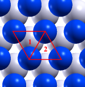
Figure 1: Geometry of the smallest three-atom clusters in the monolayer of 3$d$-atoms on $M(111)$ surface ($M$= Au, Ir): $M$-centered triangle $\Delta_{1}$ and hole-centered triangle $\Delta_{2}$.

Fig.  2 gives the parameters $J_{\Delta_{1}}(\xi_{\rm{SOC}})$ and $J_{\Delta_{2}}(\xi_{\rm{SOC}})$ calculated using Eq. (2) that was derived within the approach reported in our previous work Mankovsky et al. (2020).

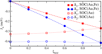
Figure 2: Three-spin chiral exchange interaction (TCI) parameters $J_{\Delta}$ calculated for Fe on Au (111) on the basis of Eq. (2) as a function of SOC scaling parameter $\xi_{SOC}$ for the smallest triangles $\Delta_{1}$ and $\Delta_{2}$. Full symbols represent the results obtained when scaling the SOC for all elements in the system, while open symbols show the results when scaling only the SOC for Au.

Note that setting the SOC scaling factor $\xi_{\rm{SOC}}=0$ implies a suppression of the SOC, while $\xi_{\rm{SOC}}=1$ corresponds to the fully relativistic case. As expected from Eq. (9), we find indeed a nearly linear variation of $J_{\Delta}(\xi_{\rm{SOC}})$ with the SOC scaling parameter $\xi_{\rm{SOC}}$ applied to all elements in the system, shown in Fig. 2 by full symbols. This shows in particular that the SOC is an ultimate prerequisite for a finite $J_{\Delta}$ and with this for the occurrence of the TCI. In addition, open symbols in Fig. 2 represent the parameters $J_{\Delta}(\xi_{\rm{SOC}})$ calculated when scaling the SOC only for Au. In this case, one can see only weak changes of the TCI, reflecting a minor impact of the SOC of the substrate on these interactions, in contrast to the DMI-like interactions that normally depend strongly on the SOC for the substrate atoms.

II.3 TCI and topological orbital moment

In a next step, we derive an expression for the above mentioned TOS on the same footing as for the TCI Mankovsky et al. (2020), i.e. within a fully relativistic approach using the multiple scattering GF formalism. By performing the calculations on the basis of the expressions derived for the TOS and for the TCI, we will demonstrate the common properties of these quantities. On the other hand, we will perform complementary calculations for the topological orbital moment (TOM) using the self-consistent embedded cluster technique, to confirm that the derived expression for the TOS gives indeed rise to the chirality-induced orbital moment. The comparison of the results confirms in particular the topological origin of the TCI.

Thus, for our purpose we represent the TOM as a sum over the products of the topological orbital susceptibility (TOS) $\chi^{\rm{TO}}_{ijk}$ determined for the triples of atoms $(ijk)$ and the corresponding scalar spin chirality $\hat{s}_{i}\cdot(\hat{s}_{j}\times\hat{s}_{k})$, that has to be seen as an effective inducing magnetic field:

$$L^{\rm{TO}} = \frac{1}{3!}\sum_{i\neq j\neq k}\chi^{\rm{TO}}_{ijk}\,[\hat{s}_{i}\cdot(\hat{s}_{j}\times\hat{s}_{k})]\;.$$ (11)

Here we restrict to the component $L^{\rm{TO}}=L_{z}^{\rm{TO}}$ along the axis $\hat{z}$ of the global frame of reference which is taken parallel to the magnetization $\vec{m}$ of the FM reference system, i.e.  $\hat{z}\|\hat{m}$ (see II.2). As one can see, Eq. (11) has by construction a form similar to the energy contribution due to the TCI, i.e. the third term in Eq. (1). Therefore we will follow Ref. [Mankovsky et al., 2020] to derive an expression for the TOS $\chi^{\rm{TO}}_{ijk}$.

As a first step, we consider the energy change in the magnetic system due to the interaction of a magnetic field with the topological orbital magnetic moment that is induced by a non-coplanar chiral magnetic structure, characterized by a nonzero scalar spin chirality $\hat{s}_{i}\cdot(\hat{s}_{j}\times\hat{s}_{k})$. The free energy change (at $T=0$ K) in the presence of an external field $\vec{B}$ is given by

$$\Delta{\cal E} = -\frac{1}{\pi}\mbox{Im}\,\mbox{Tr}\int^{E_{F}}dE(E-E_{F})\,G\hat{\cal H}_{B}G\;,$$ (12)

with the perturbation operator to $\hat{\cal H}_{B}=-\hat{\vec{l}}\cdot\vec{B}$, and $\hat{\vec{l}}$ the angular momentum operator. This way we simplify the problem by accounting for the orbital moment associated with the electrons localized on the atoms and neglecting the contribution from the non-local component of the topological orbital moment discussed, e.g., in Ref. [Hanke et al., 2016]. The reason why we are interesting here only in this part of the induced orbital moment is related to the interpretation of the TCI discussed previously Mankovsky et al. (2020). In this case the TCI is characterized by the energy change due to the interaction of the spin magnetization with the orbital moment induced by the chiral magnetic configuration.

Next, we assume a non-collinear magnetic structure in the system, which is treated as a perturbation leading to a change of the Green function $G_{0}$ for collinear magnetic system according to:

$$G = G_{0}+G_{0}VG_{0}+G_{0}VG_{0}VG_{0}+...\;,$$ (13)

where $V=V(q_{1},q_{2})$ is a perturbation due to the $2q$ spin modulation given by Eq. (29) and discussed in Ref. [Mankovsky et al., 2020] when considering the three-spin exchange interaction parameters. Using the expression in Eq. (12) we keep here only the terms giving the three-site energy contribution corresponding to the topological orbital susceptibility $\chi^{\rm{TO}}_{ijk}$:

$$\Delta{\cal E}^{(3)} = -\frac{1}{\pi}\mbox{Im}\,\mbox{Tr}\int^{E_{F}}dE(E-E_{F})\,[G_{0}VG_{0}VG_{0}\hat{\cal H}_{B}G_{0}$$ (14)

$$+\,G_{0}VG_{0}\hat{\cal H}_{B}G_{0}VG_{0}+G_{0}\hat{\cal H}_{B}G_{0}VG_{0}VG_{0}]\,.$$

As it is shown in the Appendix C, Eq. (14) can be transformed to the form

$$\Delta{\cal E}^{(3)} = \frac{1}{3}\frac{1}{\pi}[\mbox{Im}\,\mbox{Tr}\int^{E_{F}}dE[VG_{0}VG_{0}\hat{\cal H}_{B}G_{0}$$ (15)

$$+VG_{0}\hat{\cal H}_{B}G_{0}VG_{0}+\hat{\cal H}_{B}G_{0}VG_{0}VG_{0}]\;.$$

This leads to an expression for the 3-spin topological orbital susceptibility (TOS) responsible for the topological orbital moment (TOM) induced in the trimer due to the magnetic configuration characterized by a finite scalar spin chirality:

$$\chi^{\rm{TO}}_{ijk} = -\frac{1}{4\pi}\mbox{Im}\,\mbox{Tr}\int^{E_{F}}dE$$

$$\times\Big{[}\underline{T}^{i,x}\,\underline{\tau}^{ij}\underline{T}^{j,y}\,\underline{\tau}^{jk}\underline{l}_{z}^{k}\,\underline{\tau}^{ki}-\underline{T}^{i,y}\,\underline{\tau}^{ij}\underline{T}^{j,x}\,\underline{\tau}^{jk}\underline{l}_{z}^{k}\,\underline{\tau}^{ki}$$

$$-\underline{T}^{i,x}\,\underline{\tau}^{ij}\underline{l}_{z}^{j}\,\underline{\tau}^{jk}\underline{T}^{k,y}\,\underline{\tau}^{ki}\;+\underline{T}^{i,y}\,\underline{\tau}^{ij}\underline{l}_{z}^{j}\,\underline{\tau}^{jk}\underline{T}^{k,x}\,\underline{\tau}^{ki}\;$$

$$+\underline{l}_{z}^{i}\,\underline{\tau}^{ij}\underline{T}^{j,x}\,\underline{\tau}^{jk}\underline{T}^{k,y}\,\underline{\tau}^{ki}\;-\underline{l}_{z}^{i}\,\underline{\tau}^{ij}\underline{T}^{j,y}\,\underline{\tau}^{jk}\underline{T}^{k,x}\,\underline{\tau}^{ki}\Big{]}\;.$$

As it was mentioned above, the TOS given by Eq. (LABEL:Eq:TOS) characterizes the topological orbital moment along the $z$-axis in the global frame of reference, which is aligned with the magnetization direction of the FM reference system. Moreover, for the system under consideration, with all magnetic atoms equivalent, one has $L_{1}^{TO}=L_{2}^{TO}=L_{3}^{TO}=L^{TO}$ for the trimers $\Delta_{1}$ and $\Delta_{2}$. This implies that the expression for the TOS, $\chi^{\rm{TO}}_{ijk}$, given in Eq. (LABEL:Eq:TOS), gives access to the TOM $L_{i}^{TO}=L_{i,z}^{TO}$ induced on atom $i$ that has its spin orientation $\hat{s}_{i}||\hat{z}$ for the FM reference state.

Using the expression in Eq. (LABEL:Eq:TOS), calculations of the three-spin topological orbital susceptibility together with the TCI has been performed for 1ML of $3d$ metals on Ir (111) surface. Corresponding values calculated for a Fe overlayer are represented in Fig. 3 as a function of the angle $\gamma$ between the magnetization direction and the normal $\hat{n}$ to the surface plane (see Fig.  4).

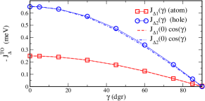
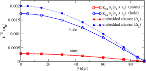
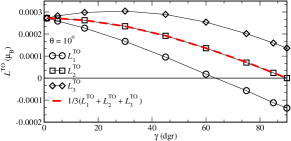
(a)
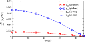
 (b)  (c)  (d)

Figure 3: (a) Three-spin chiral exchange interaction parameters $J_{\Delta}(\gamma)$ and (b) topological orbital susceptibility (TOS, for SOC = 0), calculated for Fe on Ir (111), as a function of the angle between the magnetization and normal $\hat{n}$ to the surface, for the smallest triangles $\Delta_{1}$ and $\Delta_{2}$. The dashed lines represent $J_{\Delta}(0)\,\cos(\gamma)$ (a) and $\chi^{\rm{TO}}_{\Delta}(0)\,\cos(\gamma)$ (b), respectively. To stress the relation between $J_{\Delta}$ and $\chi^{\rm{TO}}_{\Delta}$, we plot $-J_{\Delta}$ in panel (a). (c) Topological orbital moment $L^{\rm{TO}}(\gamma)$ (calculated for SOC = 0) induced by a three-site chiral spin tilting by $\theta=10^{\circ}$, for trimers $\Delta_{1}$ (red squares, centered at an Ir atom) and $\Delta_{2}$ (blue circles, centered by the hole in the Ir layer). The solid line represents the results obtained for $L^{\rm{TO}}(\gamma)=\chi^{\rm{TO}}_{\Delta}\hat{s}_{i}\cdot(\hat{s}_{j}\times\hat{s}_{k})$, while the dashed line represents the results of a direct calculations of $L^{\rm{TO}}(\gamma)$ for an embedded three-atomic Fe cluster. (d) Orbital moments $L_{i}^{\rm{TO}}(\gamma)$ on a three-atomic embedded Fe cluster $\Delta_{1}$ in Fe monolayer on Ir (111), induced at SOC = 0 due to the tilting of magnetic moments by $\theta=10^{\circ}$ with respect to the magnetization direction. The dashed line represents the average orbital moment.

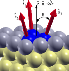
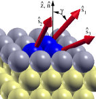
(a)
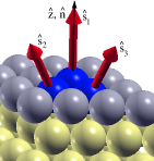
(b) (c)

Figure 4: Spin orientation in three-atomic cluster in the magnetic monolayers on Ir (111): (a) $\theta$ - the angle of tilting tilting of magnetic moments $\hat{s}_{i}$ of the trimer with respect to the magnetization direction; (b) initial spin configuration used in the calculations of the TOM on the atom $i$, for the embedded cluster; (c) $\gamma$ - the angle between the direction of spin magnetic moment $\hat{s}_{i}$ and the normal to the surface $\hat{n}_{i}$, within the plane perpendicular to the rotation axis.

These results give evidence for the common dependence of the TCI and the TOS on the flux of the spin magnetization through the triangle area. The calculations have been performed for the two smallest trimers, $\Delta_{1}$ and $\Delta_{2}$, centered at the Ir atom and the hole site in the Ir surface layer, respectively (Fig.  1). As both quantities, $J_{ijk}$ and $\chi^{\rm{TO}}_{ikj}$ , follow the permutation properties of the product $\hat{s}_{i}\cdot(\hat{s}_{j}\times\hat{s}_{k})$, we introduce the quantities $J_{\Delta}=J_{ijk}-J_{ikj}$ and $\chi^{\rm{TO}}_{\Delta}=\chi^{\rm{TO}}_{ijk}-\chi^{\rm{TO}}_{ikj}$, which allow to avoid double summation over the counter-clockwise and counter-anticlockwise contributions upon a summation over the lattice sites in the energy or orbital moment calculations. Note also that in the present case with all magnetic atoms equivalent $J_{\Delta}=J_{ijk}-J_{kji}=J_{ijk}-J_{jik}$ as well as $\chi^{\rm{TO}}_{\Delta}=\chi^{\rm{TO}}_{ijk}-\chi^{\rm{TO}}_{kji}=\chi^{\rm{TO}}_{ijk}-\chi^{\rm{TO}}_{jik}$. As one can see, both $J_{\Delta}(\gamma)$ and $\chi^{\rm{TO}}_{\Delta}(\gamma)$ are in perfect agreement with the functions $J_{\Delta}(0)\cos(\gamma)$ and $\chi^{\rm{TO}}_{\Delta}(0)\cos(\gamma)$ in line with Eq. (9) to be considered here for the situation $\hat{m}\|\hat{z}$, i.e. $\hat{m}\cdot\hat{\vec{l}}\sim\cos(\gamma)$.

The result for $\chi^{\rm{TO}}_{\Delta}$ can be compared to the pure topological orbital moment (TOM) $L^{TO}(\gamma)$ that is derived directly from the electronic structure when the SOC is suppressed. Corresponding calculations have been done for 3-atom Fe clusters ($\Delta_{1}$ or $\Delta_{2}$, as is shown in Fig. 1) embedded in a Fe monolayer on the Ir(111) surface. For this, the Fe spin moments $\hat{s}_{1},\hat{s}_{2}$, and $\hat{s}_{3}$ of the cluster given by $\hat{s}_{i}=(\sin(\theta)\,\cos(\phi_{i}),\sin(\theta)\,\sin(\phi_{i}),\cos(\theta))$ (with $\phi_{i+1}-\phi_{i}=120^{\circ}$) are tilted by the angle $\theta$ with respect to the ’average’ spin direction $\langle\hat{s}\rangle=1/3(\hat{s}_{1}+\hat{s}_{2}+\hat{s}_{3})$, as it is shown in Fig. 4.

It should be emphasized that a one-to-one comparison of two approaches is only sensible when performing the corresponding calculations under identical conditions. This implies here an orientation of the spin magnetic moment $\hat{s}_{i}$ as well as of the topological orbital moment $\hat{L}^{\rm{TO}}_{i}=\hat{L}^{\rm{TO}}_{i,z}$ on the atom $i$ along the global $\hat{z}$ axis, i.e. $\hat{L}^{\rm{TO}}_{i}||\hat{s}_{i}||\hat{z}$, identical to the conditions used within the perturbational approach. In the calculations for the embedded cluster with finite spin tilting angles, this condition can be met only for one atom of the trimer at a time, e.g. for atom $1$ (see Fig. 4 (b)). The angle $\gamma$ characterizes the relative orientation of the spin direction $\hat{s}_{1}$ and the normal $\hat{n}$ to the surface (i.e. the plane of the triangle), as is shown in Fig. 4 (c). The initial spin configuration ($\gamma=0$) used in the embedded cluster calculations shown in Fig.  4 (b) can be obtained from the configuration shown in Fig. 4 (a) by a corresponding rotation ${\cal R}_{1}$ according to $\hat{s}_{1}^{(b)}={\cal R}_{1}\hat{s}_{1}^{(a)}$, $\hat{s}_{2}^{(b)}={\cal R}_{1}\hat{s}_{2}^{(a)}$, and $\hat{s}_{3}^{(b)}={\cal R}_{1}\hat{s}_{3}^{(a)}$, such that ${\cal R}_{1}\hat{s}_{1}^{(a)}||\hat{z}$. The TOMs of atoms 2 and 3, $L_{2}^{\rm{TO}}(\gamma)$ and $L_{3}^{\rm{TO}}(\gamma)$, respectively, and their dependency on the angle $\gamma$ can be obtained from corresponding spin configurations obtained by applying the rotations ${\cal R}_{2}$ and ${\cal R}_{3}$, fixed by the requirement ${\cal R}_{2}\hat{s}_{2}^{(a)}||\hat{z}$ and ${\cal R}_{3}\hat{s}_{3}^{(a)}||\hat{z}$, respectively.

As one notices from Fig. 3 (d) for the cluster $\Delta_{1}$, the variation of the calculated TOM $L_{i}^{\rm{TO}}(\gamma)$ with the tilting angle $\gamma$ is somewhat different for the various atoms in the cluster, with the difference increasing with increasing $\theta$. Fig. 3 (c) represents by full symbols the dependence of the corresponding averaged TOM $L^{\rm{TO}}(\gamma)=1/3(L^{\rm{TO}}_{1}+L^{\rm{TO}}_{2}+L^{\rm{TO}}_{3})$ on the angle $\gamma$, with $L^{\rm{TO}}_{i}(\gamma)$ induced due to the tilting of all spin moments by the angle $\theta=10^{o}$ (see Fig.  4). Rotating the lattice, the direction of the normal vector $\hat{n}$ rotates with respect to the fixed $\hat{z}$ axis, leading to an increase of the angle $\gamma$ and to a decrease of the topological orbital moment of the 3-atomic cluster.

As one can see in Fig. 3 (c), for both considered clusters the results for $L^{\rm{TO}}(\gamma)$ are in good agreement with the TOM (given by open symbols) evaluated via $L_{\Delta}^{\rm{TO}}(\gamma)=\chi^{\rm{TO}}_{\Delta}\hat{s}_{i}\cdot(\hat{s}_{j}\times\hat{s}_{k})$ on the basis the TOS plotted in Fig. 3 (b). These findings clearly support the concept of the topological orbital susceptibility as well as the interpretation of the topological orbital moment.

In Fig. 5 we represent in addition the dependence of the directly calculated TOM on the occupation of the electronic states, which is considered for embedded Fe and Mn three-atomic clusters $\Delta_{1}$ and $\Delta_{2}$, for 1ML Fe (a) and 1ML Mn (b), respectively, on the Ir (111) surface. Such an energy-resolved representation may allow to monitor differences for the various quantities considered concerning their origin in the electronic structure. The TOM plotted in Fig. 5 by a dashed line is calculated for atom 1 in the embedded cluster with magnetic moments on the atoms tilted by $\theta=10^{\circ}$ with respect to the average spin direction $\langle\hat{s}\rangle$. In turn, $\langle\hat{s}\rangle$ is tilted by $\gamma=10^{\circ}$ to have an orientation of $\hat{s}_{1}$ along the normal $\hat{n}$ to the surface (see Fig. 4 (b)). The solid line represents the orbital moment calculated using the three-spin topological orbital susceptibility $\chi^{\rm{TO}}_{\Delta}$ scaled by the scalar spin chirality factor, i.e. $L^{\rm{TO}}_{\Delta}=\chi^{\rm{TO}}_{\Delta}\hat{s}_{1}\cdot(\hat{s}_{2}\times\hat{s}_{3})$. As one can see, both results are close to each other and the difference can be attributed to a finite $\theta$ angle in the case of the embedded cluster calculations. Comparing the results for Fe and Mn, one can also see that the different sign of the induced topological orbital moments on Fe and Mn atoms (this implies $E-E_{F}=0$ in Fig. 5) is mainly a result of a different occupation of the electronic states in these materials.

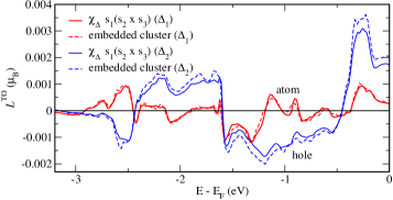
(a)
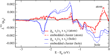
 (b)

Figure 5: Topological orbital moment (calculated for SOC = 0) induced by a three-site chiral spin tilting by $\theta=10^{\circ}$, for the smallest triangles $\Delta_{1}$ (red, centered at an Ir atom) and $\Delta_{2}$ (blue, centered by the hole in the Ir layer) in 1 ML of Fe (a) and Mn (b) on Ir (111), as a function of the occupation. The solid line represents the results obtained for $\chi^{\rm{TO}}_{\Delta}\hat{s}_{i}\cdot(\hat{s}_{j}\times\hat{s}_{k})$, while the dashed line represents the results directly calculated for the embedded three-atomic Fe cluster.

Thus, the presented results give clear evidence that the susceptibility calculated using Eq. (LABEL:Eq:TOS) characterizes an orbital moment on the atoms as a response to the effective magnetic field represented by scalar spin chirality for every three-atomic cluster. It has a form closely connected to that for the TCI and therefore should be seen as a source for the TCI according to Eq. (LABEL:Eq_INTERPR-2).

II.4 Topological spin susceptibility (TSS)

Discussing in Section II.2 the role of the SOC for the TCI using a description of the electronic structure in terms of the non-relativistic Green functions, we have shown its responsibility for the induced spin magnetic moment in the presence of a chiral magnetic structure governing the TOM. The appearance of the spin moment induced due to a chiral magnetic structure can also be demonstrated explicitly within the fully relativistic approach, that gives access to an estimate for the TCI based on Eq. (9). This can be done by introducing a ’topological’ spin susceptibility (TSS) in analogy to the TOS that is given explicitly by the expression in Eq. (LABEL:Eq:TOS). Following the discussion of the role of the SOC for the induced spin magnetization given by Eq. (8) that is based on a non-relativistic reference system one obviously has to account for the SOC when dealing with the TSS $\chi^{\rm{TS}}_{ijk}$. This is done here by working on a fully relativistic level and representing the underlying electronic structure in terms of the retarded Green function evaluated by means of the multiple-scattering formalism (see above). This approach allows to write for $\chi^{\rm{TS}}_{ijk}$ the expression:

$$\chi^{\rm{TS}}_{ijk} = -\frac{1}{4\pi}\mbox{Im}\,\mbox{Tr}\int^{E_{F}}dE$$

$$\times\Big{[}\underline{T}^{i,x}\,\underline{\tau}^{ij}\underline{T}^{j,y}\,\underline{\tau}^{jk}\underline{\sigma}_{z}^{k}\,\underline{\tau}^{ki}-\underline{T}^{i,y}\,\underline{\tau}^{ij}\underline{T}^{j,x}\,\underline{\tau}^{jk}\underline{\sigma}_{z}^{k}\,\underline{\tau}^{ki}$$

$$-\underline{T}^{i,x}\,\underline{\tau}^{ij}\underline{\sigma}_{z}^{j}\,\underline{\tau}^{jk}\underline{T}^{k,y}\,\underline{\tau}^{ki}\;+\underline{T}^{i,y}\,\underline{\tau}^{ij}\underline{\sigma}_{z}^{j}\,\underline{\tau}^{jk}\underline{T}^{k,x}\,\underline{\tau}^{ki}\;$$

$$+\underline{\sigma}_{z}^{i}\,\underline{\tau}^{ij}\underline{T}^{j,x}\,\underline{\tau}^{jk}\underline{T}^{k,y}\,\underline{\tau}^{ki}\;-\underline{\sigma}_{z}^{i}\,\underline{\tau}^{ij}\underline{T}^{j,y}\,\underline{\tau}^{jk}\underline{T}^{k,x}\,\underline{\tau}^{ki}\Big{]}\;.$$

Using this expression, $\chi^{\rm{TS}}_{\Delta}=\chi^{\rm{TS}}_{ijk}-\chi^{\rm{TS}}_{ikj}$ was calculated as a function of the SOC scaling parameter $\xi_{\rm{SOC}}$, as well as the angle $\gamma$ defined above, for 1ML Fe on Au(111) surface. Fig.  6 (a) represents the dependence of $\chi^{\rm{TS}}_{\Delta}$ on $\xi_{\rm{SOC}}$, clearly demonstrating the relativistic origin of this quantity giving rise to the corresponding contribution to the TCI (see Eq. (8)). These results can be compared with the $\xi_{\rm{SOC}}$-dependence of the TCI plotted in Fig.  2. As it has been seen in Fig. 3, when comparing $J_{\Delta}$ and $\chi^{\rm{TO}}_{\Delta}$, one finds a different sign for $J_{\Delta}$ and $\chi^{\rm{TS}}_{\Delta}$.

On the other hand, $\chi^{\rm{TS}}_{\Delta}$ should follow the angle $\gamma$ between the magnetization and surface normal $\hat{n}$, as it has been obtained for $\chi^{\rm{TO}}_{\Delta}$. As one can see in Fig.  6 (b), $\chi^{\rm{TS}}_{\Delta}(\gamma)$ is well represented by $\chi^{\rm{TS}}_{\Delta}(0)\,\cos(\gamma)$, demonstrating a common behavior of the topological spin susceptibility $\chi^{\rm{TS}}_{\Delta}$ and the TOS $\chi^{\rm{TO}}_{\Delta}$.

Using the results in Fig.  6 (a) together with the ground state spin moment $m_{\rm{Fe}}=3\mu_{\rm B}$ and the approximate exchange splitting $\Delta_{\rm{xc}}\sim 3$ eV calculated for 1 ML Fe /Au(111), one can give the crude estimate $1{\rm eV}/\mu_{\rm B}$ for the effective $B$-field $B_{\rm{eff}}\approx\Delta_{\rm{xc}}/m_{\rm{Fe}}$ giving access to the TCI connected with the TSS $\chi^{\rm{TS}}_{\Delta}$. Using Eq. (LABEL:Eq_INTERPR-2) approximated by $J_{\Delta}\approx B_{\rm{eff}}\,\chi^{\rm{TS}}_{\Delta}$, one obtains the values $J_{\Delta_{1}}\approx-0.14$ and $J_{\Delta_{2}}\approx-0.57$ meV for $\xi_{\rm{SOC}}=1$, which are in reasonable agreement with the properly calculated values shown in Fig. 2 supporting the concept of a TSS as introduced here.

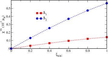
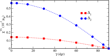
(a)  (b)

Figure 6: ’Topological’ spin susceptibility $\chi^{\rm{TS}}_{\Delta}$ calculated for trimers $\Delta_{1}$ and $\Delta_{2}$ in Fe on Au (111): (a) as a function of $\xi_{\rm{SOC}}$ and (b) as a function of the angle between the magnetization and normal $\hat{n}$ to the surface.

III Summary

To summarize, we have stressed that the TCI derived in Ref. [Mankovsky et al., 2020] is fully in line with the symmetry properties of a fully antisymmetric rank-3 tensor, specific only for this type of interaction. This interaction should be distinguished from the 4-spin DMI-like exchange interactions obtained in different order of perturbation theory and characterized by different properties with respect to a permutation of the spin indices.

We suggest an interpretation of the TCI showing its dependence on the relativistic SOC and on the TOS as a possible source. Concerning the SOC, an analytical expression based on a perturbative treatment of the SOC as well as numerical results for the TCI parameter demonstrate the role of the SOC as an ultimate source for a non-zero TCI. An expression for the TOS that reflects the topological origin of the TOS and that is very similar to that for the TCI parameters has been derived. Numerical results again demonstrate the intimate connection between both quantities.

To allow for a more detailed discussion of the TCI, the ’topological’ spin susceptibility (TSS) has been introduced as a quantity that reflects the impact of the SOC in the presence of a non-collinear magnetic structure, leading to a non-vanishing TCI. Corresponding numerical results also demonstrated for the TSS its connection with the TCI parameters.

In summary, the work presented not only revealed details of the mechanism giving rise to the TCI and its connection with related quantities but also clearly rebutted the misleading criticism raised by dos Santos Dias et al. dos Santos Dias et al. (2021).

IV Acknowledgement

Financial support by the DFG via SFB 1277 (Emergent Relativistic Effects in Condensed Matter - From Fundamental Aspects to Electronic Functionality) is gratefully acknowledged.

Appendix A Properties of the TCI with respect to time reversal

In the following we address the properties of the TCI with respect to time reversal. Considering the TCI parameter as a ’conventional’ scalar quantity invariant with respect to time reversal together with the scalar spin chirality $\hat{s}_{i}\cdot(\hat{s}_{j}\times\hat{s}_{k})$ in the third term of the spin Hamiltonian given in Eq. (1) being antisymmetric with respect to this operation one is erroneously led to the conclusion that the TCI should not contribute to the energy expansion in Eq. (1).

Concerning this, we remind here that the expression for the corresponding TCI parameter was derived in Ref. [Mankovsky et al., 2020] by considering spin tiltings as a perturbation to a FM reference system that lead to a non-collinear spin modulation. Using a representation of the electronic structure of the FM state by means of its Green function $G_{0}$ the change in energy in second-order with respect to the perturbation is given by Mankovsky et al. (2020)

$$\Delta{\cal E} = -\frac{1}{\pi}\mbox{Im}\,\mbox{Tr}\int^{E_{F}}dE(E-E_{F})\,G_{0}\,\Delta V\,G_{0}\,\Delta V\,G_{0}\;,$$

with the perturbation $\Delta V$

$$\Delta V = \sum_{i}\beta\big{(}\vec{\sigma}\cdot\hat{s}_{i}-\sigma_{z}\big{)}B_{xc}\;.$$ (19)

and all spatial arguments and corresponding integrals omitted.

As the change in energy due to an arbitrary perturbation should be invariant w.r.t. time reversal, this should hold in particular for the term given in Eq. (LABEL:Eq_Free_Energy-TCI-1A) that is second order concerning the perturbation $\Delta V$. This property is demonstrated in the following making use of the simplified version of Eq. (LABEL:Eq_Free_Energy-TCI-1A)

$$\Delta{\cal E} = -\frac{1}{\pi}\mbox{Im}\,\mbox{Tr}\int^{E_{F}}dE\,(\vec{B}_{xc}\cdot\vec{\sigma})$$ (20)

$$\times G_{0}\,\xi_{SOC}(\vec{\sigma}\cdot\hat{\vec{l}})\,G_{0}\,\Delta V\,G_{0}\,\Delta V\,G_{0}\;,$$

as given in Eq. (9), with SOC treated as a perturbation. Treating the FM state otherwise on a non-relativistic level its Green function $G_{0}$ is block-diagonal w.r.t. the spin index:

$$G_{0} = \frac{1}{2}(G_{0}^{\uparrow\uparrow}+G_{0}^{\downarrow\downarrow})+\frac{1}{2}(G_{0}^{\uparrow\uparrow}-G_{0}^{\downarrow\downarrow})\sigma_{z}$$ (21)

$$= G_{01}\sigma_{0}+G_{02}\sigma_{z}\;,$$

with $\sigma_{0}$ the unit $2\times 2$ matrix and the perturbation

$$\Delta V = \sum_{i}({\sigma}_{x}s_{x}^{i}+{\sigma}_{y}s_{y}^{i}+{\sigma}_{z}(s_{z}^{i}-1))B_{xc}\;.$$ (22)

Inserting Eqs. (21) and (22) into Eq.  (20) leads, among others, to contributions of the form

$$\sim \mbox{Im}\,\mbox{Tr}[(B_{xc}^{i}\sigma_{z})(G_{01}\sigma_{0})\,\xi_{SOC}^{i}(\sigma_{z}\hat{l}_{z})$$

$$\times G_{01}\sigma_{0}(\sigma_{x}B_{xc}^{j})\,(G_{01}\sigma_{0})(\sigma_{y}B_{xc}^{k})(G_{02}\sigma_{z})]\,,$$

which are invariant w.r.t. time reversal, as it will be shown next. A corresponding application of the time reversal operator ${\cal T}=-i\sigma_{y}{\cal K}$, with $K$ the operator of complex conjugation, to the Green function leads to

$${\cal T}(G_{01}\sigma_{0}+G_{02}\sigma_{z}){\cal T}^{-1}=(G_{01}^{*}\sigma_{0}-G_{02}^{*}\sigma_{z})\,,$$ (23)

while the operators $\Delta V$ and $(\sigma_{z}\hat{l}_{z})$ are invariant under this operation. Accordingly, one has for the contribution given above:

$$\sim \mbox{Im}\,\mbox{Tr}[(B_{xc}^{i}\sigma_{z})(G^{*}_{01}\sigma_{0})\,\xi_{SOC}^{i}(\sigma_{z}\hat{l}_{z})$$

$$\times G^{*}_{01}\sigma_{0}(\sigma_{x}B_{xc}^{j})\,(G^{*}_{01}\sigma_{0})(\sigma_{y}B_{xc}^{k})(-G^{*}_{02}\sigma_{z})]\,.$$

Making use of the specific properties of the various operators involved, one can rewrite this as:

$$\sim -\mbox{Im}\,\mbox{Tr}[(B_{xc}^{i}\sigma_{z})(G_{01}\sigma_{0})\,\xi_{SOC}^{i}(\sigma_{z}\hat{l}_{z})$$

$$\times G_{01}\sigma_{0}(\sigma_{x}B_{xc}^{j})\,(G_{01}\sigma_{0})(\sigma_{y}B_{xc}^{k})(G_{02}\sigma_{z})]^{*}\,,$$

i.e. the original expression is recovered. From this we may conclude that using Eq. (LABEL:Eq_Free_Energy-TCI-1A) within a more general fully relativistic framework contributions occur which are also invariant under time reversal and therefore characterize a stationary state of the perturbed system.

As a next step in the derivation of an expression for the TCI interaction parameters, the change in energy $\Delta{\cal E}$ in Eq. (LABEL:Eq_Free_Energy-TCI-1A) was mapped to the third term of the spin Hamiltonian given by Eq. (1).Mankovsky et al. (2020) Representing the Green function $G_{0}$ by means of the multiple scattering formalism $\Delta{\cal E}$ could be expressed by a sum over products of the TCI parameters $J_{ijk}$ given Eq. (2) and the corresponding scalar spin chirality $\hat{s}_{i}\cdot(\hat{s}_{j}\times\hat{s}_{k})$.

As it was pointed out in Section II, the derivation of the TCI term accounts automatically for the symmetry properties of the scalar spin chirality $\hat{s}_{i}\cdot(\hat{s}_{j}\times\hat{s}_{k})$. This implies that multiplying the TCI parameters by $\hat{s}_{i}\cdot(\hat{s}_{j}\times\hat{s}_{k})$ and summing over all sites should in particular be conform with the behavior under time reversal of the initial expression, i.e. the result should be invariant under time reversal. Following the discussions in Section II.3 and in Ref. [Mankovsky et al., 2020], the TCI term in the spin Hamiltonian can be contracted to a form accounting for only the counterclockwise contributions when summation over the sites:

$$H^{(3)} = -\frac{1}{3!}\sum_{i,j,k:\circlearrowleft}J_{\Delta}\hat{s}_{i}\cdot(\hat{s}_{j}\times\hat{s}_{k})\;,$$ (24)

with $J_{\Delta}=J_{ijk}-J_{ikj}$ giving the non-zero contributions to the energy. As a consequence of the mapping properties mentioned above, this parameter is antisymmetric with respect to time reversal applied to the total system. This important property was verified by electronic structure calculations with the exchange field changed in sign, that indeed led to a flip in sign for the TCI parameters as well. This property ensures that the energy given by Eq. (24) is time reversal invariant as a consequence of the properties of the corresponding energy change given by Eq. (LABEL:Eq_Free_Energy-TCI-1A). Connected with this, it should be stressed once more that the expansion leading to Eq. (LABEL:Eq_Free_Energy-TCI-1A) is based on a – in principle arbitrary – reference state (see also the corresponding discussion in Ref. [Mankovsky et al., 2020]), that addresses all other parameters in the spin Hamiltonian given by Eq. (1). Accordingly, it represents the energy landscape in the vicinity of this state in dependence on the actual spin configuration. If the reference state is changed, e.g. by time reversal, the expansion coefficients may change as well.

Finally, it is worth to compare with the energy mapping giving access to the DMI term, where the standard vector form of the DMI parameters ensures corresponding scalar energy contributions. In contrast to this situation, the time reversal antisymmetry of the TCI parameters, that nevertheless give finite energy contributions invariant under time reversal, is hidden.

Appendix B Computational details

The first-principles exchange coupling parameters are calculated using the spin-polarized relativistic KKR (SPR-KKR) Green function method H. Ebert et al. (2020); Ebert et al. (2011). The fully-relativistic mode was used except for the cases, where scaling of the spin-orbit interaction was applied. All calculations have been performed using the atomic sphere approximation (ASA), within the framework of the local spin density approximation (LSDA) to spin density functional theory (SDFT), using a parametrization for the exchange and correlation potential as given by Vosko et al. Vosko et al. (1980). A cutoff $l_{max}=2$ was used for the angular momentum expansion of the Green function. Integration over the Brillouin zone (BZ) has been performed using a $43\times 43\times 7$ k-mesh.

The calculations for 1ML of 3$d$ metals on a $M$(111) surface ($M$ = Ir, Au) have been performed in the supercell geometry with (1ML Fe/3ML $M$) layers separated by two vacuum layers. This decoupling was sufficient in the present case to demonstrate the properties of the exchange interaction parameters for the 2D system. The lattice parameter used were $a=7.22$ a.u. for fcc Ir and $a=7.68$ a.u. for fcc Au.

Appendix C TOM

Eq. (14) can be modified by using the sum rule for GF $\frac{dG}{dE}=-GG$ and integration by parts.

$$\Delta{\cal E}^{(3)} = -\frac{1}{\pi}\mbox{Im}\,\mbox{Tr}\int^{E_{F}}dE(E-E_{F})\,[VG_{0}VG_{0}\hat{\cal H}_{B}\dot{G}_{0}+VG_{0}\hat{\cal H}_{B}G_{0}V\dot{G}_{0}+\hat{\cal H}_{B}G_{0}VG_{0}V\dot{G}_{0}]\;$$ (25)

$$= \frac{1}{\pi}\mbox{Im}\,\mbox{Tr}\int^{E_{F}}dEVG_{0}VG_{0}\hat{\cal H}_{B}G_{0}+\frac{1}{\pi}\mbox{Im}\,\mbox{Tr}\int^{E_{F}}dEVG_{0}\hat{\cal H}_{B}G_{0}VG_{0}+\frac{1}{\pi}\mbox{Im}\,\mbox{Tr}\int^{E_{F}}dE\hat{\cal H}_{B}G_{0}VG_{0}VG_{0}]\;$$

$$-\frac{1}{\pi}\mbox{Im}\,\mbox{Tr}(E-E_{F})VG_{0}VG_{0}\hat{\cal H}_{B}\dot{G}_{0}|^{E_{F}}+\frac{1}{\pi}\mbox{Im}\,\mbox{Tr}\int^{E_{F}}dE(E-E_{F})\,\frac{d}{dE}[VG_{0}VG_{0}\hat{\cal H}_{B}]G_{0}\;$$

$$-\frac{1}{\pi}\mbox{Im}\,\mbox{Tr}(E-E_{F})VG_{0}VG_{0}\hat{\cal H}_{B}\dot{G}_{0}|^{E_{F}}+\frac{1}{\pi}\mbox{Im}\,\mbox{Tr}\int^{E_{F}}dE(E-E_{F})\,\frac{d}{dE}[VG_{0}\hat{\cal H}_{B}G_{0}V]G_{0}$$

$$-\frac{1}{\pi}\mbox{Im}\,\mbox{Tr}(E-E_{F})VG_{0}VG_{0}\hat{\cal H}_{B}\dot{G}_{0}|^{E_{F}}+\frac{1}{\pi}\mbox{Im}\,\mbox{Tr}\int^{E_{F}}dE(E-E_{F})\,\frac{d}{dE}[\hat{\cal H}_{B}G_{0}VG_{0}V]G_{0}\;$$

$$= \frac{1}{\pi}\mbox{Im}\,\mbox{Tr}\int^{E_{F}}dEVG_{0}VG_{0}\hat{\cal H}_{B}G_{0}+\frac{1}{\pi}\mbox{Im}\,\mbox{Tr}\int^{E_{F}}dEVG_{0}\hat{\cal H}_{B}G_{0}VG_{0}+\frac{1}{\pi}\mbox{Im}\,\mbox{Tr}\int^{E_{F}}dE\hat{\cal H}_{B}G_{0}VG_{0}VG_{0}]\;$$

$$+\frac{1}{\pi}\mbox{Im}\,\mbox{Tr}\int^{E_{F}}dE(E-E_{F})\,\frac{d}{dE}[VG_{0}VG_{0}\hat{\cal H}_{B}]G_{0}\;$$

$$+\frac{1}{\pi}\mbox{Im}\,\mbox{Tr}\int^{E_{F}}dE(E-E_{F})\,\frac{d}{dE}[VG_{0}\hat{\cal H}_{B}G_{0}V]G_{0}+\frac{1}{\pi}\mbox{Im}\,\mbox{Tr}\int^{E_{F}}dE(E-E_{F})\,\frac{d}{dE}[\hat{\cal H}_{B}G_{0}VG_{0}V]G_{0}\;$$

After partial integration, the terms without involving an integral should vanish due to the factor $(E-E_{F})|^{E_{F}}$. Taking the energy derivatives in the last three integrals, we obtain

$$-\frac{1}{\pi}\mbox{Im}\,\mbox{Tr}\int^{E_{F}}dE(E-E_{F})\,[VG_{0}VG_{0}\hat{\cal H}_{B}\dot{G}_{0}+VG_{0}\hat{\cal H}_{B}G_{0}V\dot{G}_{0}+\hat{\cal H}_{B}G_{0}VG_{0}V\dot{G}_{0}]\;$$ (26)

$$= \frac{1}{\pi}\mbox{Im}\,\mbox{Tr}\int^{E_{F}}dE\,VG_{0}VG_{0}\hat{\cal H}_{B}G_{0}+\frac{1}{\pi}\mbox{Im}\,\mbox{Tr}\int^{E_{F}}dE\,VG_{0}\hat{\cal H}_{B}G_{0}VG_{0}+\frac{1}{\pi}\mbox{Im}\,\mbox{Tr}\int^{E_{F}}dE\,\hat{\cal H}_{B}G_{0}VG_{0}VG_{0}\;$$

$$+\frac{1}{\pi}\mbox{Im}\,\mbox{Tr}\int^{E_{F}}dE(E-E_{F})\,[V\dot{G}_{0}VG_{0}\hat{\cal H}_{B}]G_{0}+\frac{1}{\pi}\mbox{Im}\,\mbox{Tr}\int^{E_{F}}dE(E-E_{F})\,[VG_{0}V\dot{G}_{0}\hat{\cal H}_{B}]G_{0}\;$$

$$+\frac{1}{\pi}\mbox{Im}\,\mbox{Tr}\int^{E_{F}}dE(E-E_{F})\,[V\dot{G}_{0}\hat{\cal H}_{B}G_{0}V]G_{0}+\frac{1}{\pi}\mbox{Im}\,\mbox{Tr}\int^{E_{F}}dE(E-E_{F})\,[VG_{0}\hat{\cal H}_{B}\dot{G}_{0}V]G_{0}$$

$$+\frac{1}{\pi}\mbox{Im}\,\mbox{Tr}\int^{E_{F}}dE(E-E_{F})\,[\hat{\cal H}_{B}\dot{G}_{0}VG_{0}V]G_{0}+\frac{1}{\pi}\mbox{Im}\,\mbox{Tr}\int^{E_{F}}dE(E-E_{F})\,[\hat{\cal H}_{B}G_{0}V\dot{G}_{0}V]G_{0}\;.$$

Using the invariance of the trace of matrix product w.r.t. cyclic permutations, one can combine the latter integrals and bring them to the left. With this one arrives at the expression

$$\Delta{\cal E}^{(3)} = \frac{1}{3}\frac{1}{\pi}[\mbox{Im}\,\mbox{Tr}\int^{E_{F}}dEVG_{0}VG_{0}\hat{\cal H}_{B}G_{0}$$ (27)

$$+\mbox{Im}\,\mbox{Tr}\int^{E_{F}}dEVG_{0}\hat{\cal H}_{B}G_{0}VG_{0}$$

$$+\mbox{Im}\,\mbox{Tr}\int^{E_{F}}dE\hat{\cal H}_{B}G_{0}VG_{0}VG_{0}]\;.$$

Representing the Green functions in terms of multiple-scattering formalism, this expression can be reduced to the expression

$$\Delta{\cal E}^{(3)} = \frac{1}{3}\frac{1}{\pi}\sum_{i\neq j\neq k}\mbox{Im}\,\mbox{Tr}\int^{E_{F}}dE\,$$

$$\times\bigg{[}\langle Z_{i}|\hat{\cal H}_{B}|Z_{i}\rangle\tau_{ij}\langle Z_{j}|\delta v_{j}|Z_{j}\rangle\tau_{jk}\langle Z_{k}|\delta v_{k}|Z_{k}\rangle\tau_{ki}$$

$$+\langle Z_{i}|\delta v_{i}|Z_{i}\rangle\tau_{ij}\langle Z_{j}|\hat{\cal H}_{B}|Z_{j}\rangle\tau_{jk}\langle Z_{k}|\delta v_{k}|Z_{k}\rangle\tau_{ki}$$

$$+\langle Z_{i}|\delta v_{i}|Z_{i}\rangle\tau_{ij}\langle Z_{j}|\delta v_{j}|Z_{j}\rangle\tau_{jk}\langle Z_{k}|\hat{\cal H}_{B}|Z_{k}\rangle\tau_{ki}\bigg{]}\;,$$

which has a similar form as the expression for the energy associated with the three-spin chiral interactions given previouslyMankovsky et al. (2020). Here the perturbation $\delta v_{i}$ in the system is associated with the non-coplanar magnetic texture. Following the idea used to derive the expression for the TCIMankovsky et al. (2020), we create a $2q$ spin modulation according to

$$\hat{s}_{i} = (\sin(\vec{q}_{1}\cdot\vec{R}_{i})\,\cos(\vec{q}_{2}\cdot\vec{R}_{i}),\;\sin(\vec{q}_{2}\cdot\vec{R}_{i}),$$ (29)

$$\cos(\vec{q}_{1}\cdot\vec{R}_{i})\,\cos(\vec{q}_{2}\cdot\vec{R}_{i}))\;,$$

which is characterized by two wave vectors, $\vec{q}_{1}$ and $\vec{q}_{2}$, orthogonal to each other. Taking the second-order derivatives with respect to $\vec{q}_{1}$ and $\vec{q}_{2}$ in the limit $q_{1}\to 0$, $q_{2}\to 0$, Eq. (LABEL:Eq_Free_Energy-TCI-5) can be reduced to the form

$$\Delta{\cal E}^{(3)} = \frac{1}{3!}\sum_{i\neq j\neq k}\hat{s}_{i}\cdot(\hat{s}_{j}\times\hat{s}_{k})\frac{1}{4\pi}\mbox{Im}\,\mbox{Tr}\int^{E_{F}}dE$$

$$\times\Big{[}\underline{T}^{i,x}\,\underline{\tau}^{ij}\underline{T}^{j,y}\,\underline{\tau}^{jk}\underline{H}_{B}^{k}\,\underline{\tau}^{ki}-\underline{T}^{i,y}\,\underline{\tau}^{ij}\underline{T}^{j,x}\,\underline{\tau}^{jk}\underline{H}_{B}^{k}\,\underline{\tau}^{ki}$$

$$-\underline{T}^{i,x}\,\underline{\tau}^{ij}\underline{H}_{B}^{j}\,\underline{\tau}^{jk}\underline{T}^{k,y}\,\underline{\tau}^{ki}\;+\underline{T}^{i,y}\,\underline{\tau}^{ij}\underline{H}_{B}^{j}\,\underline{\tau}^{jk}\underline{T}^{k,x}\,\underline{\tau}^{ki}\;$$

$$+\underline{H}_{B}^{i}\,\underline{\tau}^{ij}\underline{T}^{j,x}\,\underline{\tau}^{jk}\underline{T}^{k,y}\,\underline{\tau}^{ki}\;-\underline{H}_{B}^{i}\,\underline{\tau}^{ij}\underline{T}^{j,y}\,\underline{\tau}^{jk}\underline{T}^{k,x}\,\underline{\tau}^{ki}\Big{]}\;.$$

That in turn, taking into account $\hat{\cal H}_{B}=-\hat{\vec{l}}\cdot\vec{B}$, leads to the topological orbital moment

$$L^{\rm{TO}} = \frac{1}{3!}\sum_{i\neq j\neq k}\chi^{\rm{TO}}_{ijk}\hat{s}_{i}\cdot(\hat{s}_{j}\times\hat{s}_{k})$$

$$= -\frac{1}{3!}\sum_{i\neq j\neq k}\hat{s}_{i}\cdot(\hat{s}_{j}\times\hat{s}_{k})\frac{1}{4\pi}\mbox{Im}\,\mbox{Tr}\int^{E_{F}}dE$$

$$\times\Big{[}\underline{T}^{i,x}\,\underline{\tau}^{ij}\underline{T}^{j,y}\,\underline{\tau}^{jk}\underline{l}_{z}^{k}\,\underline{\tau}^{ki}-\underline{T}^{i,y}\,\underline{\tau}^{ij}\underline{T}^{j,x}\,\underline{\tau}^{jk}\underline{l}_{z}^{k}\,\underline{\tau}^{ki}$$

$$-\underline{T}^{i,x}\,\underline{\tau}^{ij}\underline{l}_{z}^{j}\,\underline{\tau}^{jk}\underline{T}^{k,y}\,\underline{\tau}^{ki}\;+\underline{T}^{i,y}\,\underline{\tau}^{ij}\underline{l}_{z}^{j}\,\underline{\tau}^{jk}\underline{T}^{k,x}\,\underline{\tau}^{ki}\;$$

$$+\underline{l}_{z}^{i}\,\underline{\tau}^{ij}\underline{T}^{j,x}\,\underline{\tau}^{jk}\underline{T}^{k,y}\,\underline{\tau}^{ki}\;-\underline{l}_{z}^{i}\,\underline{\tau}^{ij}\underline{T}^{j,y}\,\underline{\tau}^{jk}\underline{T}^{k,x}\,\underline{\tau}^{ki}\Big{]}\;.$$

References

- Wang et al. (2010) H. Wang, P.-W. Ma, and C. H. Woo, Phys. Rev. B 82, 144304 (2010).
- Kvashnin et al. (2016) Y. O. Kvashnin, R. Cardias, A. Szilva, I. Di Marco, M. I. Katsnelson, A. I. Lichtenstein, L. Nordström, A. B. Klautau, and O. Eriksson, Phys. Rev. Lett. 116, 217202 (2016).
- Connolly and Williams (1983) J. W. D. Connolly and A. R. Williams, Phys. Rev. B 27, 5169 (1983).
- Drautz and Fähnle (2004) R. Drautz and M. Fähnle, Phys. Rev. B 69, 104404 (2004).
- Antal et al. (2008) A. Antal, B. Lazarovits, L. Udvardi, L. Szunyogh, B. Újfalussy, and P. Weinberger, Phys. Rev. B 77, 174429 (2008).
- Uhl et al. (1994) M. Uhl, L. M. Sandratskii, and J. Kübler, Phys. Rev. B 50, 291 (1994).
- Halilov et al. (1998) S. V. Halilov, H. Eschrig, A. Y. Perlov, and P. M. Oppeneer, Phys. Rev. B 58, 293 (1998).
- Sandratskii and Bruno (2002) L. M. Sandratskii and P. Bruno, Phys. Rev. B 66, 134435 (2002).
- Heide et al. (2008) M. Heide, G. Bihlmayer, and S. Blügel, Phys. Rev. B 78, 140403 (2008).
- Liechtenstein et al. (1984) A. I. Liechtenstein, M. I. Katsnelson, and V. A. Gubanov, J. Phys. F: Met. Phys. 14, L125 (1984).
- Liechtenstein et al. (1987) A. I. Liechtenstein, M. I. Katsnelson, V. P. Antropov, and V. A. Gubanov, J. Magn. Magn. Materials 67, 65 (1987).
- Pajda et al. (2000) M. Pajda, J. Kudrnovský, I. Turek, V. Drchal, and P. Bruno, Phys. Rev. Lett. 85, 5424 (2000).
- Udvardi et al. (2003) L. Udvardi, L. Szunyogh, K. Palotás, and P. Weinberger, Phys. Rev. B 68, 104436 (2003).
- Ebert and Mankovsky (2009a) H. Ebert and S. Mankovsky, J. Phys.: Cond. Mat. 21, 326004 (2009a).
- Kittel (1960) C. Kittel, Phys. Rev. 120, 335 (1960).
- Köbler et al. (1996) U. Köbler, R. Mueller, L. Smardz, D. Maier, K. Fischer, B. Olefs, and W. Zinn, Zeitschrift für Physik B Condensed Matter 100, 497 (1996).
- Müller-Hartmann et al. (1997) E. Müller-Hartmann, U. Köbler, and L. Smardz, Journal of Magnetism and Magnetic Materials 173, 133 (1997).
- Parihari and Pati (2004) D. Parihari and S. K. Pati, Phys. Rev. B 70, 180403 (2004).
- Greiter and Thomale (2009) M. Greiter and R. Thomale, Phys. Rev. Lett. 102, 207203 (2009).
- Greiter et al. (2014) M. Greiter, D. F. Schroeter, and R. Thomale, Phys. Rev. B 89, 165125 (2014).
- Bauer et al. (2014) B. Bauer, L. Cincio, B. P. Keller, M. Dolfi, G. Vidal, S. Trebst, and A. W. W. Ludwig, Nature Communications 5, 5137 (2014).
- Fedorova et al. (2015) N. S. Fedorova, C. Ederer, N. A. Spaldin, and A. Scaramucci, Phys. Rev. B 91, 165122 (2015).
- Kartsev et al. (2020) A. Kartsev, M. Augustin, R. F. L. Evans, K. S. Novoselov, and E. J. G. Santos, npj Computational Materials 6, 120 (2020).
- Lászlóffy et al. (2019) A. Lászlóffy, L. Rózsa, K. Palotás, L. Udvardi, and L. Szunyogh, Phys. Rev. B 99, 184430 (2019).
- Paul et al. (2020) S. Paul, S. Haldar, S. von Malottki, and S. Heinze, Nature Communications 1, 475 (2020).
- Mara Gutzeit (2021) S. M. S. H. Mara Gutzeit, Soumyajyoti Haldar, arXiv:2104.10371v1 (2021).
- Brinker et al. (2019) S. Brinker, M. dos Santos Dias, and S. Lounis, New Journal of Physics 21, 083015 (2019).
- Brinker et al. (2020) S. Brinker, M. dos Santos Dias, and S. Lounis, Phys. Rev. Research 2, 033240 (2020).
- Mankovsky et al. (2020) S. Mankovsky, S. Polesya, and H. Ebert, Phys. Rev. B 101, 174401 (2020).
- Shallcross et al. (2005) S. Shallcross, A. E. Kissavos, V. Meded, and A. V. Ruban, Phys. Rev. B 72, 104437 (2005).
- Buruzs et al. (2008) A. Buruzs, L. Szunyogh, and P. Weinberger, Phil. Mag. 88, 2615 (2008).
- Szilva et al. (2017) A. Szilva, D. Thonig, P. F. Bessarab, Y. O. Kvashnin, D. C. M. Rodrigues, R. Cardias, M. Pereiro, L. Nordström, A. Bergman, A. B. Klautau, and O. Eriksson, Phys. Rev. B 96, 144413 (2017).
- Cardias et al. (2020) R. Cardias, A. Szilva, M. M. Bezerra-Neto, M. S. Ribeiro, A. Bergman, Y. O. Kvashnin, J. Fransson, A. B. Klautau, O. Eriksson, and L. Nordström, Scientific Reports 10, 20339 (2020).
- Streib et al. (2021) S. Streib, A. Szilva, V. Borisov, M. Pereiro, A. Bergman, E. Sjöqvist, A. Delin, M. I. Katsnelson, O. Eriksson, and D. Thonig, arXiv:2103.04726v3 (2021).
- (35) R. Cardias, A. Bergman, A. Szilva, Y. O. Kvashnin, J. Fransson, A. B. Klautau, O. Eriksson, and L. Nordström, arXiv:2003.04680 .
- Secchi et al. (2013) A. Secchi, S. Brener, A. Lichtenstein, and M. Katsnelson, Annals of Physics 333, 221 (2013).
- Hoffmann and Blügel (2020) M. Hoffmann and S. Blügel, Phys. Rev. B 101, 024418 (2020).
- dos Santos Dias et al. (2021) M. dos Santos Dias, S. Brinker, A. Lászlóffy, B. Nyári, S. Blügel, L. Szunyogh, and S. Lounis, Phys. Rev. B 103, L140408 (2021).
- Grytsiuk et al. (2020) S. Grytsiuk, J.-P. Hanke, M. Hoffmann, J. Bouaziz, O. Gomonay, G. Bihlmayer, S. Lounis, Y. Mokrousov, and S. Blügel, Nature Communications 11, 511 (2020).
- Ruiz-Tolosa and Enrique (2005) J. R. Ruiz-Tolosa and C. Enrique, From Vectors to Tensors (Springer, Berlin, Heidelberg, New York, 2005).
- Ebert and Mankovsky (2009b) H. Ebert and S. Mankovsky, Phys. Rev. B 79, 045209 (2009b).
- Rose (1961) M. E. Rose, Relativistic Electron Theory (Wiley, New York, 1961).
- Ebert et al. (2016) H. Ebert, J. Braun, D. Ködderitzsch, and S. Mankovsky, Phys. Rev. B 93, 075145 (2016).
- Nakamura et al. (2003) K. Nakamura, T. Ito, and A. J. Freeman, Phys. Rev. B 68, 180404 (2003).
- Freeman et al. (2004) A. Freeman, K. Nakamura, and T. Ito, Journal of Magnetism and Magnetic Materials 272-276, 1122 (2004), proceedings of the International Conference on Magnetism (ICM 2003).
- dos Santos Dias et al. (2016) M. dos Santos Dias, J. Bouaziz, M. Bouhassoune, S. Blügel, and S. Lounis, Nature Communications 7, 13613 (2016).
- Thonhauser (2011) T. Thonhauser, International Journal of Modern Physics B 25, 1429 (2011), https://doi.org/10.1142/S0217979211058912 .
- Hanke et al. (2016) J.-P. Hanke, F. Freimuth, A. K. Nandy, H. Zhang, S. Blügel, and Y. Mokrousov, Phys. Rev. B 94, 121114 (2016).
- H. Ebert et al. (2020) H. Ebert et al., The Munich SPR-KKR package, version 8.5, https://www.ebert.cup.uni-muenchen.de/en/software-en/13-sprkkr (2020).
- Ebert et al. (2011) H. Ebert, D. Ködderitzsch, and J. Minár, Rep. Prog. Phys. 74, 096501 (2011).
- Vosko et al. (1980) S. H. Vosko, L. Wilk, and M. Nusair, Can. J. Phys. 58, 1200 (1980), http://www.nrcresearchpress.com/doi/pdf/10.1139/p80-159 .