Electrochemical removal of amphoteric ions

Abstract

Several harmful or valuable ionic species present in sea, brackish and wastewaters are amphoteric, and thus their properties depend on the local water pH. Effective removal of these species can be challenging by conventional membrane technologies, necessitating chemical dosing of the feedwater to adjust its pH. Capacitive deionization (CDI) is an emerging membraneless technique for water treatment and desalination, based on electrosorption of salt ions into charging microporous electrodes. CDI cells show strong internally-generated pH variations during operation, and thus CDI can potentially remove amphoteric species without chemical dosing. However, development of this technique is inhibited by the complexities inherent to coupling of pH dynamics and amphoteric ion properties in a charging CDI cell. Here, we present a novel theoretical framework predicting the electrosorption of amphoteric species in flow-through electrode CDI cells. We demonstrate that such a model enables deep insight into factors affecting amphoteric species electrosorption, and conclude that important design rules for such systems are highly counter-intuitive. For example, we show both theoretically and experimentally that for boron removal the anode should be placed upstream, which runs counter to accepted wisdom in the CDI field. Overall, we show that to achieve target separations relying on coupled, complex phenomena, such as in the removal of amphoteric species, a theoretical CDI model is essential.

1 Introduction

Global fresh water scarcity is increasing due to population growth, increased water consumption per capita, and shrinking freshwater bodies due to climate change and over-extraction.[1, 2, 3] About 4 billion people are subject to severe water scarcity for at least one month per year,[4] and increasing parts of the global population are predicted to face chronic water scarcity.[5] Consequently, there has been increasing demand for efficient water treatment and desalination technologies over the past few decades.[6, 7] Water treatment also provides an opportunity for recovery of valuable elements from feedwater.[8, 9]

Commonly used technologies for water treatment and desalination are pressure-driven membrane-based separation technologies, such as reverse-osmosis (RO),[10, 11, 7] nanofiltration and ultrafiltration. [12, 13] During operation, mechanical energy is invested in pumping and pressurizing feedwater through the membrane, while ions and other compounds can be retained by the membrane. Two important mechanisms for the rejection of ions and molecules by membranes are size-expulsion,[14, 15], and charge repulsion,[14, 15, 16]. An ion’s volume includes its hydration shell, which often plays an important role in rejection.

The charge of several common pollutants and valuable solutes depends on the solution pH, and such species are characterized as amphoteric. Arsenic acid, As(V), and arsenous acid, As(III), are toxic amphoteric ions, and therefore should be removed during drinking water treatment.[17, 18, 19] Boron is an amphoteric ion which is considered toxic when at high concentrations in water,[20, 21] and which can be detrimental to plant growth.[22, 23, 24] Phosphate and ammonia should be removed from wastewater, as these amphoteric ions can negatively affect the surface water quality when present at high concentrations.[1, 25, 26, 27]. They are also desirable to recover during water treatment, [8, 28, 27, 9, 29] as they are important nutrients.[30] Acetate is a small organic acid and amphoteric, and is often removed and recovered during sugar production.[31, 32] As the hydration shell of amphoteric ions varies with their charge, the rejection of amphoteric species by membranes is generally pH-dependent, and may be highly challenging under certain conditions.[33]

Boron is an example of an amphoteric ion that can be poorly rejected in membrane-based systems. Boron is present in protonated form, B(OH)3, under standard pH conditions (pH of surface water is generally between 7 and 8), and can dissociate into B(OH)4- and BO(OH)3^2- at higher pH, see Fig. 1a. Since B(OH)3 is not charged, the hydration of the molecule is weak, and B(OH)3 can pass through the pores of an RO membrane, resulting in a low removal rate. The removal is generally only around 50-60% for feedwater with a pH below 8, but values ranging from 10-30% have been reported as well.[34, 35, 36, 37, 38] To increase boron removal with RO, common practice is to pass desalinated water multiple times through an RO membrane.[39, 40, 41] Another practice is to dose, after the first RO pass and before the second RO pass, a caustic solution to adjust the pH to higher values.[41, 42, 43] This adjustment results in boron primarily appearing within B(OH)4- and BO(OH)3^2-, species which are blocked by the RO membrane due to their larger hydrated size.

Capacitive deionization (CDI) is an emerging membraneless electrochemical separation technology used for water treatment and desalination. Typical CDI cells employ a cyclic process of alternatingly charging and discharging a pair of nanoporous carbon electrodes. During the charging step, ions are removed from the feedwater by electrosorption into the electrodes, and during the discharge step the electrodes are regenerated and the ions are released into the brine. Several cell designs for CDI have been proposed, including flow-by electrode CDI, membrane CDI, and flow-through electrode (FTE) CDI,[44] the latter schematically shown in Fig. 1b. In FTE CDI, the solution flows through the electrodes,[45, 44] which allows the use of a thinner separator compared to other cell designs, enabling reduced cell resistance[46] and faster desalination, but can lead to enhanced electrode degradation.[47, 48] Recent breakthroughs in CDI focus on its ability to remove ions selectively from polluted feedwaters,[49, 50, 51, 52, 53, 54, 55, 56] and new electrode materials based on intercalation compounds or Faradaic reactions.[57, 58, 59, 60, 61]

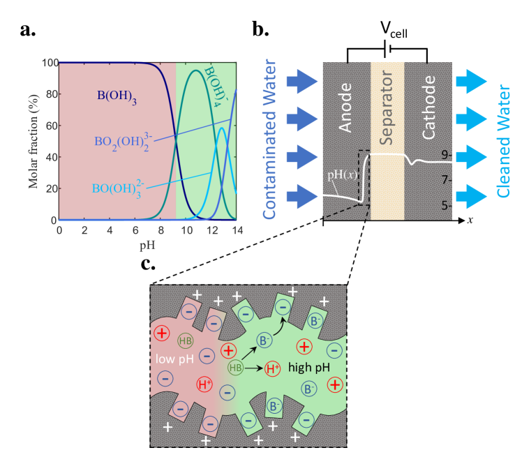
Figure 1: Schematic demonstrating boron removal by a CDI cell. a. Boron is amphoteric in water, and plotted is the molar fraction of the various boron-containing species as a function of water pH. b. A CDI cell with an anode placed upstream, and a snapshot of the developed pH profile within the electrodes. c. A snapshot of ion and charge distributions near the anode/separator interface, showing boric acid dissociation and electrosorption.

During charging of a CDI cell with nanoporous carbon electrodes, large pH differences naturally develop in the cell, with pH values as high as $\sim$ 10 reported in the cathode and as low as $\sim$ 3 in the anode.[62, 63] Several mechanisms have been proposed to explain these pH differences, including side-reactions such as oxygen reduction,[64, 65, 66, 62, 63] the difference in diffusion coefficients between ionic species present in solution, and electrosorption of H+ and OH-.[62, 48, 66] Thus far, one theoretical model was developed including pH effects in membrane CDI,[66] with significant deviations between model and experiment, and no models have been developed for membraneless CDI, to our knowledge. Thus, pH effects and dynamics in CDI remain poorly understood, and the in-situ generated pH gradients in a CDI cell remain largely unexploited.

In the present work, we utilize these strong differences in local pH of charging CDI cells to ensure amphoteric species are charged and can be electrosorbed into the electrodes, see Fig. 1b-c. Despite the presence of several experimental studies,[67, 68, 69, 70, 71, 72, 73, 74, 75, 76] no theory has been developed to predict and guide the removal of amphoteric species by CDI. Given the complexities involving pH dynamics in CDI, a validated model is essential to unlock the enormous potential of CDI to remove amphoteric ions without chemical additives to adjust feed pH. We here provide such a theory, to our knowledge the first model coupling electrosorption into nanopores to local pH dynamics and acid-base equilibria, by a transient description of multi-component ion transport in porous electrodes, and amphoteric ions present in the feed. We show that our model predicts highly counter-intuitive design rules for removal of amphoteric species by CDI, which we validate experimentally using boron as a case study. In the future, the theoretical framework presented here can be adapted to any other amphoteric species, and can be used to improve the understanding of pH dynamics in electrochemical systems.

2 Results and Discussion

In this section, we employ the theoretical framework presented in the Materials and Methods section. This model captures local pH variations in the CDI cell, and the electrosorption of amphoteric species present in the feedwater. We consider an FTE CDI cell depicted in Fig. 5a, with feedwater containing both a salt and an amphoteric species. To electrosorb the amphoteric species effectively, the species must be present in an ionic form while in the CDI cell. For example, ammonia is largely protonated and positively charged at neutral and low pH values ($\mathrm{p}K_{\mathrm{a}}$=9.25) , while boron is largely deprotonated and negatively charged at high pH conditions ($\mathrm{p}K_{\mathrm{a}}$=9.24), see Fig. 1a. Thus, to remove boron, a high pH is required in the anode, and for ammonia removal, neutral or low pH is required in the cathode.

Here, we illustrate the theory by analyzing the electrosorption of boron as a case study, and compare the theoretical predictions to experimental data. As we do not expect the local pH in the cell to exceed the value of 10, we exclude the species BO(OH)_3^2- and BO2(OH)2^3- from our analysis (Fig. 1a), and account only for B(OH)3, which hence will be referred to as HB, and B(OH)4-, which will be denoted B-. The feedwater we consider has a composition resembling the effluent from an RO system, so with relatively low salt concentration on the order of $\sim 1\ \rm{mM}$, a boron feed concentration of 0.37 mM, and a near-neutral feed pH $\left(6\leq\rm{pH_{F}}\leq 7\right)$.[77]

2.1 Electrode order affects local pH and boron removal

The order of the electrodes in an FTE CDI cell may directly affect local pH values, and ultimately may be a central consideration for successful boron removal. Conventional wisdom is that during CDI cell charging, the solution in the cathode macropores becomes basic and in the anode acidic.[64, 62] Naively, we may expect that at feed velocities characterized by Peclet number of order unity and above (${\rm Pe}\equiv v_{\mathrm{w}}l_{\mathrm{e}}/D_{\mathrm{s}}$, with $v_{\mathrm{w}}$ the superficial flow velocity, $l_{\mathrm{e}}$ the electrode thickness, and $D_{\mathrm{s}}$ the effective salt diffusion coefficient, see Table 1), the cathode should be placed upstream so the high pH solution can be advected into the anode, allowing for boron electrosorption. As we will show, model and experimental results both prove that this expectation is not correct.

In Fig. 2a-c we compare the predicted salt, boron, potential, and pH profiles of two cell configurations operated with Pe=3 and a charging voltage of 1.0 V (Tables 1 and 2). In the first configuration, the cathode is placed upstream (cat-an, solid lines), and for the second the cathode is placed downstream (an-cat, dashed lines). Fig. 2a shows predicted pH profiles (left y-axis, black lines) and macropore salt concentration (right y-axis, blue lines), defined by $c_{\mathrm{mA,NaCl}}\equiv\tfrac{1}{2}(c_{\mathrm{mA,Na^{+}}}+c_{\mathrm{mA,Cl^{-}}})$, both as a function of the location scaled by $l_{\mathrm{e}}$, and at $t/\tau_{\mathrm{D}}=2$, where $\tau_{\mathrm{D}}$ is the dimensionless time, defined as $l_{\mathrm{e}}^{2}/D_{\mathrm{s}}$. In Fig. 2a we see that for both configurations the salt concentration decreases along the upstream electrode in flow direction, and is essentially completely depleted throughout most of the downstream electrode. For the cat-an configuration, the pH profile includes three distinct regions. First, in the upstream electrode (cathode) near the inlet, there is a relatively high pH of approximately 7.5. In the downstream half of the cathode, a sharp pH decrease to approximately 3.7 is observed. The latter feature is a novel observation to our knowledge, and runs contrary to conventional wisdom that the solution in the charging cathode is alkaline.[78, 62] Then, towards the downstream region of the anode pH rises again to values of approximately 4.6. For the an-cat configuration, the pH profile is changed significantly, with a pH of approximately 5.8 in the upstream part of the anode, followed by a sharp increase in pH close to the separator to about 8.6. The latter feature is again a novel observation and contrary to conventional wisdom that solution in the charging anode is acidic.[78, 62] Decreasing pH values are predicted along the rest of the cathode, reaching a value of about 6.9 at the effluent.

Thus, results of Fig. 2a indicate that the anode should be placed upstream for effective boron removal, counter to our naive expectation. To gain more insight into this counter-intuitive behavior, Fig. 2b shows predicted profiles for potential, $\phi$, (left y-axis, black lines) and $c_{\mathrm{mA,\ce{B-}}}$ (right y-axis, blue lines) at $t/\tau_{\mathrm{D}}=2$. The potential profiles in Fig. 2b for both configurations are not symmetric about the cell midline, where in both cases $\phi$ changes sign in the downstream electrode. This is likely due to the strong salt depletion in the downstream electrode, as presented in Fig. 2a. Further, we see that for both configurations, by far the strongest electric field (potential gradient) occurs just downstream of the separator. As expected based on the results of Fig. 2a, $c_{\mathrm{mA,\ce{B-}}}$ for the cat-an configuration is approximately zero across the cell, as the pH is too low for significant boric acid deprotonation. However, for the an-cat configuration we observe low values along most of the upstream electrode (anode), followed by a strong increase near the anode/separator interface, reaching a maximum value of 0.21 mM at the separator as boric acid is deprotonated in that region, followed by a decrease and lower values of approximately 0.04 mM in the cathode. Thus, due to strong boric acid deprotonation within the anode, the an-cat configuration is highly promising for effective boron electrosorption.

We argue that the counter-intuitive findings of these predictions are due to the complicated interplay between salt depletion, H+ and OH- electrosorption and electromigration, and water splitting, see Eq. 19. For example, for the cat-an configuration, the low salt concentration $\left(c_{\mathrm{mA,NaCl}}<0.2\ \mathrm{mM}\right)$ in the anode leads to enhanced OH- electrosorption into the micropores and can cause increases in local H+ production due to water splitting. The strong electric field in the upstream-end of the anode can increase H+ electromigration into the cathode, reducing pH in the cathode as seen in Fig. 2a. Detailed study of such mechanisms are beyond the scope of the current work, but are important to unravel in future works which seek to optimize electrosorption of amphoteric species, such as boron, by CDI.

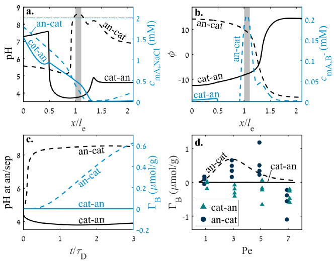
Figure 2: Predictions and experimental results for a FTE CDI cell with cathode placed upstream (cat-an, solid lines) or downstream (an-cat, dashed lines), for $c_{\mathrm{F}}$=2 mM, $c_{\mathrm{F,B}}$=0.37 mM and $V_{\mathrm{ch}}$=1.0 V, where in panels a-c Pe=3. a. Predicted pH (left y-axis, black lines) and macropore salt concentration (right y-axis, blue lines) profiles in the FTE CDI cell. b. Predicted scaled potential (left y-axis, black lines) and B- macropore concentration (right y-axis, blue lines) profiles. The profiles in panels a and b are snapshots at $t/\tau_{D}=2$, the gray-shaded rectangles represent the separator, and the horizontal dash-dotted blue line in panel a represents the feed salt concentration. c. Predicted pH at the anode/separator interface (left y-axis, black lines), and electrosorbed boron (right y-axis, blue lines), both as a function of dimensionless time. d. Predicted and measured boron boron electrosorption for an effluent collection time of 10 min as a function of Pe for cat-an (solid line, triangles) and an-cat (dashed line, circles) configurations.

To explore the dynamics of our model CDI cell, Fig. 2c shows the predicted pH at the anode/separator interface (left y-axis, black lines) and the cumulative electrosorbed boron by the cell, $\Gamma_{\mathrm{B}}$, defined in Eq. 25 (right y-axis, blue lines), as functions of dimensionless time for the cat-an (solid lines) and an-cat (dashed lines) configurations. The pH at the anode/separator interface is a crucial metric, which can be used to rapidly assess whether the cell will be effective towards boric acid dissociation and boron ion electrosorption at the anode. For both configurations, we observe rapid development of the pH values at the anode/separator interface, within about $t/\tau_{\mathrm{D}}$ of 0.4, to near steady values. Thus, for essentially the entire charging process, the an-cat configuration is predicted to be capable of electrosorbing boron, as the solution at the anode/separator interface is alkaline. For the cat-an configuration, as expected the predicted boron electrosorption is negligible at all times during charging, while for the an-cat configuration, it is monotonically increasing for $t/\tau_{\mathrm{D}}\geq$ 0.5, reaching a value of $0.62\text{\,}\mathrm{\SIUnitSymbolMicro}\mathrm{mol}\mathrm{/}\mathrm{g}$ at $t/\tau_{\mathrm{D}}$=3.

To validate the model predictions, we compare our theoretical findings with experimental data (see Materials and Methods for details). In Fig. 2d we plot theoretical (lines) and experimental (markers) values of $\Gamma_{\mathrm{B}}$, as a function of Pe. We include predictions and measurements for boron removal in both cat-an (solid line, triangles) and an-cat (dashed line, circles) configurations. The theoretical predictions in Fig. 2d show effective boron removal by the cell for the an-cat configuration, where no removal is expected for the cat-an configuration. While comparing theory and experimental results in Fig. 2d, we observe a good agreement for the an-cat configuration for low and moderate flow velocities $\left(3\leq\rm{Pe}\leq 5\right)$, measuring a boron removal of around $0.50\text{\,}\mathrm{\SIUnitSymbolMicro}\mathrm{mol}\mathrm{/}\mathrm{g}$, although for high values $\left(\rm{Pe}=7\right)$ we obtain negative values of $\Gamma_{\mathrm{B}}$, indicating boron desorption. As predicted by the model, for all conditions tested, no significant boron removal was achieved in the cat-an configuration. Thus, the counter-intuitive prediction that an-cat is the preferred electrode order was also confirmed experimentally.

2.2 Optimum charging voltage for boron removal

We further investigate the effects of charging voltage on pH dynamics and boron removal, now focusing on a cell with an-cat electrode order. Naively, we would expect to observe monotonic increase of boron removal with the charging voltage, as previous experimental observations show that pH perturbations in the anode and cathode become more extreme with increased cell voltage.[62, 63] In Fig. 3a-c we show the predicted salt and charge dynamics of a cell operated with $c_{\mathrm{F}}$=2 mM, Pe=3 and charging voltages of 0.6 V (solid lines), 1.0 V (dashed lines) and 1.4 V (dotted lines), see Tables 1 and 2 for other model parameters used. Fig. 3a shows the profiles of pH (left y-axis, black lines) and macropore salt concentration (right y-axis, blue lines) at $t/\tau_{\mathrm{D}}=2$. The pH profiles for all investigated charging voltages bear significant similarities: acidic values along most of the anode, followed by a strong rise near the anode/separator interface to alkaline values, and maintaining high pH across the separator and much of the cathode. For relatively high $V_{\mathrm{ch}}$, we observe a distinct pH local minima in the cathode near to the separator, with a minima of 8.0 for $V_{\mathrm{ch}}$=1.0 V, and much lower value of 6.3 for $V_{\mathrm{ch}}$=1.4 V. The salt concentration profiles for all the analyzed charging voltages are similar to the profile presented in Fig. 2a for the an-cat configuration.

Fig. 3b presents the profiles of $\phi$ (left y-axis, black lines) and macropore B- concentration (right y-axis, blue lines) at $t/\tau_{\mathrm{D}}=2$. As with Fig. 2b, the potential profiles are similarly asymmetric about the cell midline, and the electric field is highest in the cathode near the separator. The location of the strongest electric field coincides with sharp local minima in pH as seen in Fig. 3a for the case of $V_{\mathrm{ch}}$=1.4 V. For all cell voltages analyzed, the macropore B- concentration is near zero along most of the anode, followed by a sharp increase near the anode/separator interface. For $V_{\mathrm{ch}}$=0.6 V, the maximum of 0.075 mM occurs in the cathode. However, the maximum values of 0.21 mM for $V_{\mathrm{ch}}$=1.0 V and 0.13 mM for $V_{\mathrm{ch}}$=1.4 V are developed in the separator. Counter-intuitively, these results suggest that boron electrosorption will be less effective at $V_{\mathrm{ch}}$=1.4 V than $V_{\mathrm{ch}}$=1.0 V due to the slightly higher pH values developed for the latter case.

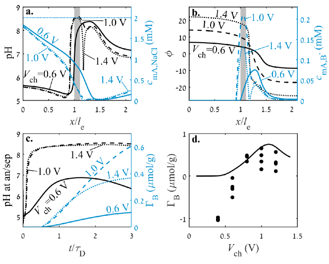
Figure 3: Predictions and experimental results for a FTE CDI cell with $c_{\mathrm{F}}$=2 mM, $c_{\mathrm{F,B}}$=0.37 mM and Pe=3. Predictions in panels a.-c. are for $V_{\mathrm{ch}}=0.6\ V$ (solid lines), 1.0 V (dashed lines) and 1.4 V (dotted lines). a. Predicted pH (left y-axis, black lines) and macropore salt concentration (right y-axis, blue lines) profiles. b. Predicted scaled potential (left y-axis, black lines) and B- macropore concentration (right y-axis, blue lines) profiles. The profiles in panels a and b are for $t/\tau_{D}=2$, gray rectangles represent the separator, and the horizontal dash-dotted blue line in panel a represents feed salt concentration. c. Predicted pH at the anode/separator interface (left -axis, black lines) and electrosorbed boron (right y-axis, blue lines), both as a function of dimensionless time. d. Predicted (lines) and measured (markers) boron electrosorption for an effluent collection time of 10 min versus $V_{\mathrm{ch}}$.

To probe the effect of $V_{\mathrm{ch}}$ on the cell dynamics, in Fig. 3c we plot predicted pH at the anode/separator interface (left y-axis, black lines) and cumulative electrosorbed boron (right y-axis, blue lines), both as a function of dimensionless time for charging voltages of 0.6 V (solid lines), 1.0 V (dashed lines) and 1.4 V (dotted lines). For $V_{\mathrm{ch}}$=0.6 V we observe relatively low pH values at this interface for the entire charging step, never surpassing 7. However, for $V_{\mathrm{ch}}$=1.0 V and 1.4 V we can see a fast increase in pH at at early times, $t/\tau_{D}<0.4$, followed by approximately steady pH at this interface of about 8.5 for $V_{\mathrm{ch}}$=1.4 V and slightly higher value of 8.6 for 1.0 V. The cumulative boron electrosorption for all the cases is monotonically increasing, but at $V_{\mathrm{ch}}$=0.6 V the amount of electrosorbed boron is the lowest, $\Gamma_{\mathrm{B}}$=$0.11\text{\,}\mathrm{\SIUnitSymbolMicro}\mathrm{mol}\mathrm{/}\mathrm{g}$ at $t/\tau_{\mathrm{D}}$=3, followed by $0.37\text{\,}\mathrm{\SIUnitSymbolMicro}\mathrm{mol}\mathrm{/}\mathrm{g}$ for $V_{\mathrm{ch}}$=1.4 V, and $0.60\text{\,}\mathrm{\SIUnitSymbolMicro}\mathrm{mol}\mathrm{/}\mathrm{g}$ at $V_{\mathrm{ch}}$=1.0 V.

Next, we compare these theoretical predictions to experimental measurements, see Materials and Methods for more details about the experimental setup. In Fig. 3d we compare between theoretical (lines) and experimental (circles) values of $\Gamma_{\mathrm{B}}$ as a function of $V_{\mathrm{ch}}$. The theoretical predictions in Fig. 3d show an optimum charging voltage for boron removal of approximately 1.1 V. Good quantitative agreements between theory and experiments are obtained for high charging voltages ($V_{\mathrm{ch}}\geq$0.8 V), however at lower voltages the model predicts no boron storage, and the experiments show significant boron desorption. Overall, experiments and theory agree and show that increasing cell voltage does not necessarily lead to improved boron removal, and that an optimum cell voltage is achieved at around 1 V.

2.3 Effects of feed salt concentration and velocity on local pH

Having established that our theory captures key trends in boron electrosorption, we now investigate theoretically the effects of the flow velocity and feed salt concentration on pH dynamics and boron electrosorption. In Fig. 4a-d we present the analysis of a cell operated with solely salt in the feedwater and no amphoteric species, where in Fig. 4e-f we include boric acid in the feed. Model parameters used are tabulated in Tables 1 and 2. Fig. 4a presents the effect of the flow velocity, quantified by Pe, on the pH in the cell, plotting the pH (left y-axis, black lines) and macropore salt concentration (right y-axis, blue lines) profiles at $t/\tau_{D}=3$, for Pe=0.2 (solid lines), 1 (dashed lines) and 5 (dotted lines), all with $c_{\mathrm{F}}$=0.5 mM and $V_{\mathrm{ch}}$=1.0 V. For the case of low flow velocity, ${\rm Pe}=0.2$, in Fig. 4a, we observe very low salt concentrations across the whole cell, with near zero concentration in the separator. For moderate and high flow velocities, Pe=1 and 5, we observe a decreasing salt concentration across the anode, followed by very low concentration throughout the cathode. For all Pe tested, the pH profiles of the three analyzed cases show low pH values across most of the anode of approximately 6.0, and high pH values of approximately 8.5 across the separator and cathode.

Fig. 4b plots the pH (left y-axis, black lines) and macropore salt concentration (right y-axis, blue lines) profiles at $t/\tau_{D}=3$, for $c_{\mathrm{F}}=0.1\ \mathrm{mM}$ (solid lines), 0.5 mM (dashed lines), and 5 mM (dotted lines), all with ${\rm Pe}=1$ and $V_{\mathrm{ch}}$=1.0 V. For all salt concentrations, the pH profiles in Fig. 4b are similar: low pH values in the anode, followed by an increase near the anode/separator interface, and high pH values across the separator and the cathode. The pH at the anode/separator interface for $c_{\mathrm{F}}=0.1\ \mathrm{mM}$ is 8.3, 9.1 for $5\ \mathrm{mM}$ and 9.3 for $c_{\mathrm{F}}=2\ \mathrm{mM}$. To conveniently visualize that the effect of flow velocity and feed salt concentration on the important metric of pH at the anode/separator interface, in Fig. 4c and d we present colormaps and contour plots at $t/\tau_{\mathrm{D}}=0.5$ (Fig. 4c) and $t/\tau_{\mathrm{D}}=3$ (Fig. 4d). For early times the pH at the anode/separator interface is above 9 for most of the investigated parameter range, while for later times, the pH decreases somewhat at high values of $c_{\mathrm{F}}$ and Pe. However, over almost the entire parameter set investigated here, pH at the anode/separator interface is high enough to be suitable for significant boric acid dissociation and boron electrosorption at the anode.

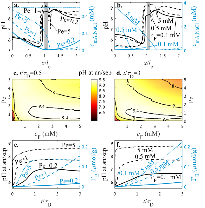
Figure 4: Predictions for a FTE CDI cell with with NaCl-containing feedwater (a.-d.), or NaCl and boron-containing feedwater (e.-f.), with $V_{\mathrm{ch}}$=1.0 V. a. and b. Predicted pH (left y-axes, black lines) and macropore salt concentration (right y-axes, blue lines) profiles at $t/\tau_{D}=3$, where the gray rectangles represent the separator, and the horizontal dash-dotted blue line in a. represents the feed salt concentration. a. and e. Results for ${\rm Pe}=0.2$ (solid lines), 1 (dashed lines), and 5 (dotted lines), all with $c_{\mathrm{F}}$=0.5 mM. c. and f. Results for $c_{\mathrm{F}}$=0.1 mM (solid lines), 0.5 mM (dashed lines), and 5 mM (dotted lines), all with Pe=1. c. and d. Predicted pH at the anode/separator interface as a function of $c_{\mathrm{F}}$ and Pe at $t/\tau_{\mathrm{D}}=0.5$ (c.) and $t/\tau_{\mathrm{D}}=3$ (d.).

In Fig. 4e and f we extend the analysis for a feedwater with both NaCl and boron. Fig. 4e and f plot the pH at the anode/separator interface (left y-axis, black lines) and $\Gamma_{\mathrm{B}}$ (right y-axis, blue lines), both as a function of dimensionless time. Fig. 4e shows results for Pe=0.2 (solid lines), 1 (dashed lines) and 5 (dotted lines), all with $c_{\mathrm{F}}$=0.5 mM, while Fig. 4f shows results for $c_{\mathrm{F}}=0.1$ mM (solid lines), 0.5 mM (dashed lines), and 5 mM (dotted lines), all with Pe=1.

The pH values for Pe=0.2 in Fig. 4e are relatively low along the whole process, followed by the values for Pe=1, where for Pe=5 a strong pH increase is observed at early times reaching values above 8.5, followed by a steady and moderate increase. For Pe=0.2 and 1 we observe monotonic increase of $\Gamma_{\mathrm{B}}$ along the investigated time range, while for Pe=5 we observe strong boron removal at $t/\tau_{\mathrm{D}}\leq$0.9, followed by a steady value. The pH values at the anode in Fig. 4e are similar to the values presented for a cell operated without boron, where the presence of boron in the system restrains the pH rise. The boron removal values presented in Fig. 4e are logical, as the boron adsorption increases with pH. However, the lack of boron removal for Pe=5 at $t/\tau_{\mathrm{D}}>$0.9 may be due to the relatively high Cl- concentration near the anode/separator interface, which competes with boron to be stored in anode micropores.

The pH values for $c_{\mathrm{F}}$=0.1 mM presented in Fig. 4f are low at all times during charging, significantly higher pH seen for $c_{\mathrm{F}}$=0.5 mM. For $c_{\mathrm{F}}$=5 mM the pH reaches about 8.7 for $t/\tau_{\mathrm{D}}\geq$ 0.2. Thus, boron removal is very low for $c_{\mathrm{F}}$=0.1 mM, while for $c_{\mathrm{F}}$ of 0.5 mM and 5 mM higher values are predicted, reaching $0.22\text{\,}\mathrm{\SIUnitSymbolMicro}\mathrm{mol}\mathrm{/}\mathrm{g}$ at $t/\tau_{\mathrm{D}}$=3 for the latter case.

3 Conclusions

The removal of amphoteric species from water is important, both for water purification and for resource recovery, but is often challenging to accomplish with conventional membrane-based technologies. We here propose and establish the theory for removal of amphoteric species by membraneless capacitive deionizaton (CDI) cells, which generate large internal pH gradients during cell charging. Our proposed theoretical framework extends traditional CDI theory by including both pH dynamics and amphoteric species in the feedwater that can protonate or deprotonate depending on local pH. Both our model and validating experiments showed important and counter-intuitive design rules for removal of boron, our example amphoteric species. Despite conventional wisdom in CDI, we found that the anode should be placed upstream to achieve effective boron removal, and that increasing cell voltage does not necessarily lead to improved boron removal. Although generally good agreement between experiments and theory were attained for key trends, quantitative differences between theory and experiments are hypothesized to be due to Faradaic side-reactions which were not included in the model presented here. In the future, the framework here can be extended to include Faradaic side-reactions to enhance its quantitative predictive capabilities, and applied to any number of amphoteric species.

4 Materials and Methods

4.1 Experimental apparatus

Activated carbon cloth (ACC-5092-15, Kynol GmbH, Germany) with $600\text{\,}\mathrm{\SIUnitSymbolMicro m}$ thickness, $0.53\text{\,}\mathrm{m}\mathrm{L}\mathrm{/}\mathrm{g}$ specific micropore volume, and approximately $1400\text{\,}\mathrm{m}\mathrm{{}^{2}}\mathrm{/}\mathrm{g}$ surface area (latter two values from Ref. [56]) was used as the electrode material. This material was characterized in a number of previous CDI studies.[78, 79, 53, 80, 56] The carbon was cut into electrode squares with a cross-sectional area of $6.25\text{\,}{\mathrm{cm}}^{2}$. Electrodes were rinsed with deionized water, dried for 3 hr at $80\text{\,}\mathrm{\SIUnitSymbolCelsius}$, then weighed immediately.

The FTE CDI cell was described and illustrated in Ref. [56]. Briefly, the cell consists of two electrodes electronically isolated by a separator (Omnipore JHWP PTFE membrane, Merck, $65\text{\,}\mathrm{\SIUnitSymbolMicro m}$ thickness) cut to a size of $2.7\text{\,}\mathrm{cm}$ $\times$ $2.7\text{\,}\mathrm{cm}$. Graphite current collectors contact the posterior side of each electrode, and a grid of holes was milled into each collector to allow water passage. The upstream reservoir is located just ahead of the first current collector, and likewise the downstream reservoir is located just behind the second collector. The cell is enclosed on both sides by milled PVDF blocks, which contain ports for fluid flow and air evacuation. Compressible ePTFE gaskets seal the cell.

Feedwater composed of 0.37 mM ($4\text{\,}\mathrm{m}\mathrm{g}\mathrm{/}\mathrm{L}$) boric acid (Bio-Lab, Israel) and 2 mM NaCl ($>$99.5%, SDFCL, India) was prepared with $18.2\text{\,}\mathrm{M\SIUnitSymbolOhm}$ deionized water (Synergy, Merck KGaA, Germany). Prior to each CDI experiment, the feedwater was purged of dissolved oxygen by nitrogen gas bubbling for 20 minutes in a 0.5 L glass feed reservoir under stirring. A peristaltic pump (Masterflex 07551-30, Cole-Parmer, USA) then transported the feedwater through the conductivity sensor (Tracedec 390-50, Innovative Sensor Technologies GmbH, Austria to measure its initial conductivity, and a pH electrode (iAquatrode Plus Pt1000, Metrohm AG, Switzerland) was dipped into the feed reservoir to measure the initial feedwater pH.

In each CDI experiment, the peristaltic pump supplied feedwater to the CDI cell. The electrodes were initially discharged at 0 V with a voltage source (2400 Source Meter, Keithley Instruments, USA) while feedwater flowed through the cell until the current was negligible. The cell was then charged for 12 min at a given voltage and flow rate and discharged for 30 min at 0 V for three consecutive charge-discharge cycles. The long discharge step allowed the cell to re-equilibrate with the incoming feedwater before the subsequent charge step. Effluent conductivity was measured for the duration of the experiment. During the charge step of the 3rd (limit) cycle, the effluent solution was collected continuously for 10 min beginning from the moment when the dynamic effluent conductivity decreased below the feed conductivity value. Feedwater samples were also collected for analysis.

The boron concentrations in the collected samples were measured with the Azomethine-H method of López et al.[81] Absorbance was measured at 414 nm against a blank reference solution with an Evolution 300 spectrophotometer (Thermo Fisher Scientific, USA). Boron concentration was interpolated from a calibration curve constructed from the absorbances of 1-5 $\text{\,}\mathrm{m}\mathrm{g}\mathrm{/}\mathrm{L}$ standard solutions.

4.2 Theory

To describe the transport and removal of amphoteric species in an electrochemical cell employing porous carbon electrodes, we present a novel theoretical framework that describes the joint processes: I) ion transport due to advection, diffusion, and migration, II) ongoing association and dissociation equilibrium reactions of water and amphoteric species, and III) ion adsorption in electrical double layers (EDLs), including the presence of pH-dependent chemical surface groups. In the porous electrodes, we distinguish two different types of pores: macropores, which serve as transport pathways, see Fig. 5b, and micropores, in which ions are electrosorbed into overlapping EDLs, see Fig. 5c and d. These definitions are based on pore function, whereas the conventionally used definitions by the IUPAC are based on pore size.[82]

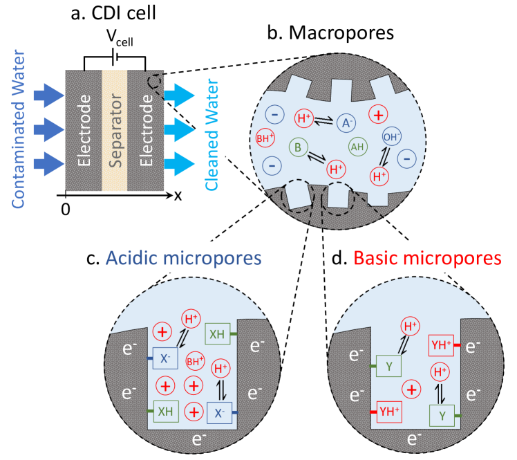
Figure 5: Schematic overview of a CDI cell for the removal of amphoteric species. a. The FTE CDI cell consists of two electrodes separated by a separator, through which feedwater, which contains inert and amphoteric ions, flows while the electrodes electrosorb the ions. b. In the macropores, which serve as transport pathways, the local pH across the cell is evaluated, as well as the pH-dependent chemical equilibria between the amphoteric ions, and the H+ and OH- ions. c. and d. Micropores for ion adsorption into overlapping EDLs, filled by electrosorbed ions, and chemical surface groups with pH-dependent chemical charge. Several regions are considered, including acidic (c.) and basic (d.) regions.

To describe ion electrosorption in the porous carbon electrodes, we use the multi-equilibria amphoteric modified Donnan (ME-amph-mD) model.[83] This model is an extended version of the amphoteric modified Donnan (amph-mD) model, which has been extensively validated and shown to describe experimental data well.[54, 66] The amph-mD model considers the presence of a fixed number of chemical groups in the micropores, but omits the pH-dependency of these groups. In contrast, the ME-amph-mD model includes this pH-dependency, based on the models presented by Hemmatifar et al. and Oyarzun et al.[84, 85]

In the ME-amph-mD model, as well as in the amph-mD model, we consider several micropore regions: $m$ acidic regions and $n$ basic regions. In these micropore regions, surface groups with a pH-dependent charge are present. In the present work, we only consider monovalent chemical groups, reacting only with H+ or OH- ions, see Fig. 5c and d. We follow Persat et al.[86] and Hemmatifar et al.,[84] and consider a local chemical equilibrium between the protonated and deprotonated surface groups, which dependents on an equilibrium constant, $K_{a}$, and the local pH. In the acidic regions, negatively charged chemical surface groups are present, marked as $\ce{X-}$ in Fig. 5c, while in the basic regions, positively charged groups are present, marked as $\ce{YH+}$ in Fig. 5d. All these groups can be in a protonated or deprotonated state, dependent on the local pH in the respective micropore region. The state of the groups is found by the following chemical equilibrium reactions

$$\ce{X_{\it i}H\rightleftharpoons X_{\it i}-+H+}, K_{\ce{X_{\it i}H}}=\frac{\left[\ce{X_{\it i}-}\right]\cdot\left[\ce{H+}\right]}{\left[\ce{X_{\it i}H}\right]}$$ (1)

$$\ce{Y_{\it j}H+\rightleftharpoons Y_{\it j}+H+}, K_{\ce{Y_{\it j}H+}}=\frac{\left[\ce{Y_{\it j}}\right]\cdot\left[\ce{H+}\right]}{\left[\ce{Y_{\it j}H+}\right]}$$ (2)

where $K_{\ce{X_{i}H}}$ is the equilibrium constant of the $i$-th acidic region, and $K_{\ce{Y_{j}H+}}$ is the equilibrium constant of the $j$-th basic group. The chemical surface charge in these regions is pH-dependent, i.e., only a part of the total concentration of chemical surface groups is charged, and the rest are not charged. The acidic groups are negatively charged in their deprotonated state, and the basic surface groups are positively charged in their protonated state. The chemical surface charge is thus given by

$$\sigma_{\mathrm{chem,X_{\it i}}} =-\frac{c_{\mathrm{chem,X_{\it i},t}}}{1+c_{\mathrm{mi,\ce{H+},X_{\it i}}}/K_{\ce{X_{\it i}H}}}$$ (3)

$$\sigma_{\mathrm{chem,Y_{\it j}}} =\frac{c_{\mathrm{chem,Y_{\it j},t}}}{1+K_{\ce{Y_{\it j}H+}}/c_{\mathrm{mi,\ce{H+},Y_{\it j}}}}$$ (4)

where subscript $\ce{X_{i}}$ refers to the $i$-th acidic region, and $\ce{Y_{j}}$ to the $j$-th basic region, and where $\sigma_{\mathrm{chem},R}$ is the chemical surface charge, $c_{\mathrm{chem},R,\mathrm{t}}$ the total concentration of chemical surface groups, and $c_{\mathrm{mi,\ce{H+}},R}$ is the H+ concentration, all in the micropore in region $R$.

The ion concentration of the $i$-th ion in the micropores in region $R$ is given by considering local thermodynamic equilibrium

$$c_{\mathrm{mi},i,R}=c_{\mathrm{mA},i}\cdot\mathrm{exp}\left(-z_{i}\Delta\phi_{\mathrm{D},R}\right)$$ (5)

where $c_{\mathrm{mi},i,R}$ is the concentration in region $R$, $c_{\mathrm{mA},i}$ is the concentration in the macropores, $z_{i}$ is the ion valence, and $\Delta\phi_{\mathrm{D},R}$ is the Donnan potential in region $R$. The Donnan potential, as all other potentials presented below, can be multiplied by the thermal voltage, given by $V_{\mathrm{T}}\equiv k_{\mathrm{B}}T/e$, to arrive at a dimensional voltage, where ${k_{\mathrm{B}}}$ is the Boltzmann constant, $T$ is the absolute temperature and $e$ is the elementary charge.

We define the total micropore concentration for each species by summing over all micropore regions the concentration of free ions in the micropores and the concentration of ions chemically bound to the surface groups. The total concentration is calculated by

$$c_{\mathrm{mi,tot},i}=\sum_{R}\alpha_{\mathrm{mi},R}\left(c_{\mathrm{mi},i,R}+\beta_{\mathrm{mi},i,R}\cdot c_{\mathrm{chem},R,\mathrm{t}}\right)$$ (6)

where $\alpha_{\mathrm{mi},R}$ is the fraction of the total micropore volume, that is in region $R$, and $\beta_{\mathrm{mi},i,R}$ is the ratio between the concentration of $i$-th ion bound to the chemical groups, and the total concentration of chemical groups, both in region $R$. Here, we account for chemical groups reacting only with H+ or OH- ions, so $\beta_{\mathrm{mi},i,R}=0$ holds for all species, except for H^+ and OH^-. Moreover, under the convention of considering only acid dissociation constants, see Eqs. 1 and 2, we note that $\beta_{\mathrm{mi},\ce{OH-},R}=0$, and

$$\beta_{\mathrm{mi},\ce{H+},R}=\frac{1}{1+K_{R}/c_{\mathrm{mi,\ce{H+}},R}}$$ (7)

where $K_{R}$ is the reaction constant of the chemical group in region $R$. Next, by combining Eq. 7 with Eqs. 1 and 2 the following expressions hold

$$\sigma_{\mathrm{chem,X_{i}}}=-\left(1-\beta_{\mathrm{mi},\ce{H+}\mathrm{X_{i}}}\right)\cdot c_{\mathrm{chem,X_{i},t}}$$ (8)

$$\sigma_{\mathrm{chem,Y_{j}}}=\beta_{\mathrm{mi},\ce{H+}\mathrm{Y_{j}}}\cdot c_{\mathrm{chem,Y_{j},t}}.$$ (9)

For each micropore region, we can calculate the ionic charge, given by

$$\sigma_{\mathrm{ionic},R}=\sum_{i}z_{i}\cdot c_{\mathrm{mi},i,R}.$$ (10)

Moreover, for each micropore region, a charge balance holds, which states that the sum of electronic charge, ionic charge and chemical charge is equal to zero

$$\sigma_{\mathrm{elec},R}+\sigma_{\mathrm{chem},R}+\sigma_{\mathrm{ionic},R}=0$$ (11)

where $\sigma_{\mathrm{elec},R}$ is the electronic charge in region $R$. The electronic charge is related to the Stern capacitance and the Stern potential by

$$\sigma_{\mathrm{elec},R}\cdot F=V_{\mathrm{T}}\cdot C_{\mathrm{S},R}\Delta\phi_{\mathrm{S},R}$$ (12)

where $F$ is the Faraday constant, $C_{\mathrm{S},R}$ is the Stern capacitance and $\Delta\phi_{\mathrm{S},R}$ is the Stern potential, both in region $R$.

For each electrode, and each micropore region, the summation of $\Delta\phi_{\mathrm{D},R}$ and $\Delta\phi_{\mathrm{S},R}$ is equal to the difference between the electrical potential in the electrode and the macropores. Therefore, we evaluate the following equation for each electrode

$$\phi_{\mathrm{E},e}-\phi_{\mathrm{mA}}=\Delta\phi_{\mathrm{D},R}+\Delta\phi_{\mathrm{S},R}$$ (13)

where $\phi_{\mathrm{mA}}$ is the dimensionless potential in the macropores, subscript “E” refers to the electrode region and subscript “e” refers to the electrode type, which is either the anode (an) or the cathode (cat). The values of $\phi_{\mathrm{E,an}}$ and $\phi_{\mathrm{E,cat}}$ are related to the cell voltage by the expression

$$V_{\mathrm{T}}(\phi_{\mathrm{E,an}}-\phi_{\mathrm{E,cat}})=V_{\mathrm{cell}}-I\cdot\rm{EER}$$ (14)

where $I$ is the electric current through the cell and EER refers to external electronic resistance [46].

To describe the transport of ions, we use the Nernst-Planck equation

$$J_{i}=v_{\mathrm{w}}c_{\mathrm{mA},i}-D_{\mathrm{mA},i}\left(\frac{\partial c_{\mathrm{mA},i}}{\partial x}+z_{i}\cdot c_{\mathrm{mA},i}\frac{\partial\phi_{\mathrm{mA}}}{\partial x}\right)$$ (15)

where $J_{i}$ is the superficial flux of ionic species $i$, $v_{\mathrm{w}}$ is the superficial velocity of the water phase, $D_{\mathrm{mA},i}$ is the effective ion diffusion coefficient in the macropores, and $x$ is the location in the cell, as shown in Fig. 5a. The parameter $D_{\mathrm{mA},i}$ is given by $D_{\mathrm{mA},i}\equiv D_{\infty,i}\cdot p_{\mathrm{mA}}/\tau_{\mathrm{mA}}$, where $D_{\infty,i}$ is the diffusion coefficient in free solution, $p_{\mathrm{mA}}$ is the macropore porosity and $\tau_{\mathrm{mA}}$ is the macropore tortuosity.

Mass conservation holds in the electrodes. Therefore, we evaluate the following mass balance equation

$$p_{\mathrm{mA}}\frac{\partial c_{\mathrm{mA},i}}{\partial t}+p_{\mathrm{mi}}\frac{\partial c_{\mathrm{mi,tot},i}}{\partial t}=-\frac{\partial J_{i}}{\partial x}+\Gamma_{i}$$ (16)

where $p_{\mathrm{mi}}$ is the micropore porosity, and $c_{\mathrm{mi,tot},i}$ is given by Eq. 6. Moreover, $\Gamma_{i}$ is the production rate of the $i$-th ion due to acid-base equilibrium reactions in the bulk. For inert ions, which do not participate in acid-base equilibria, such as Na+ and Cl-, $\Gamma_{i}=0$. For amphoteric ions, the value of $\Gamma_{i}$ is almost always different from zero, and the value is often unknown. However, although $\Gamma_{i}$ is unknown, an explicit evaluation of $\Gamma_{j}$ is not required, as presented in the next paragraph.

Let us illustrate how $\Gamma_{i}$ disappears, following the approach described in Refs. [87, 88, 89] We derive a total mass balance equation for a group of species, marked by $G$, which includes all species that are in chemical equilibrium with each other. At each position in the system, the summation of the production rates, $\Gamma_{i}$, of all species in a group, $G$, is equal to zero, i.e., $\sum\limits_{i\in G}\Gamma_{i}=0$. Consequently, summing Eq. 16 over the individual species within group $G$, all $\Gamma_{i}$ terms cancel out, resulting in the following mass balance equation

$$\sum_{i\in G}{\left(p_{\mathrm{mA}}\frac{\partial c_{\mathrm{mA},i}}{\partial t}+p_{\mathrm{mi}}\frac{\partial c_{\mathrm{mi,tot},i}}{\partial t}\right)}=-\sum_{i\in G}\frac{\partial J_{i}}{\partial x}.$$ (17)

The approach presented by Eq. 17 eliminates the $\Gamma_{i}$ terms from the system of equations that is solved. To solve the resulting set of equations, we assume the acid-base equilibrium reactions between ionic species within a group are infinitely fast, i.e., these species are in chemical equilibrium. Thus we evaluate, at each position in the system and at each moment, the following chemical equilibrium conditions for the group

$$K_{i}=\frac{\left[\mathrm{P}_{i}\right]\cdot\left[\ce{H+}\right]}{\left[\mathrm{R}_{i}\right]}$$ (18)

where $K_{i}$ is the equilibrium constant, $\mathrm{P}_{i}$ is the product, and $\mathrm{R}_{i}$ is the reactant, all of the $i$-th acid-base equilibrium reaction. Similarly, we consider the water dissociation equilibrium, H2O ⇌H+ + OH-, with the equilibrium constant

$$K_{\mathrm{w}}=\left[\ce{H+}\right]\cdot\left[\ce{OH-}\right].$$ (19)

Now, we consider electroneutrality at each position in the macropores and in the separator

$$\sum_{i}z_{i}\cdot c_{\mathrm{mA},i}=0.$$ (20)

Next, we derive the charge balance by multiplying Eq. 16 by $z_{i}$, and summing the resulting equations over all ionic species, including H+ and OH-

$$p_{\mathrm{mi}}\frac{\partial}{\partial t}\sum_{i}z_{i}\cdot c_{\mathrm{mi,tot},i}=-\frac{\partial}{\partial x}\sum_{i}z_{i}J_{i}.$$ (21)

Only the micropores contribute to the left hand side of Eq. 21, as charge does not accumulate in the macropores, see Eq. 20. Furthermore, charge conservation in the equilibrium reactions eliminates the term associated with the reaction rates. Also, by expanding Eq. 21, and substituting Eqs. 8 and 9 into it, the charge balance can be written as

$$p_{\mathrm{mi}}\sum_{R}{\alpha_{\mathrm{mi},R}\bigg{(}\frac{\partial\sigma_{\mathrm{chem},R}}{\partial t}+\frac{\partial\sigma_{\mathrm{ionic},R}}{\partial t}\bigg{)}}=-\frac{\partial J_{\mathrm{ch}}}{\partial x}$$ (22)

where $J_{\mathrm{ch}}$ is the superficial charge flux, defined as $J_{\mathrm{ch}}\equiv\sum\limits_{i}{z_{i}\cdot J_{i}}$. In the separator, $J_{\mathrm{ch}}$ is related to $I$, by the expression $I=F\cdot A_{\mathrm{c}}\cdot J_{\mathrm{ch}}$, where $A_{\mathrm{c}}$ is the electrode cross section area.

Next, we describe ion transport across the separator, a thin layer of insulating porous material allowing the transport of water and ions. To do so, we use a mass balance equation for all the inert ions (Eq. 16), a mass balance for all amphoteric groups (of the form of Eq. 17), the charge balance (Eq. 22), the electroneutrality condition (Eq. 20), and the chemical equilibrium equations (Eqs. 18 and 19). In the aforementioned equations, the subscript “mA” is replaced by “sep”, referring to the separator, and $p_{\mathrm{mi}}=0$.

On both separator/electrode interfaces, we consider continuity of flux for the inert ions, $\left.J_{\mathrm{sep},i}\right|_{\mathrm{sep/e}}=\left.J_{\mathrm{e},i}\right|_{\mathrm{sep/e}}$, where the subscripts “$\mathrm{sep}$” and “$\mathrm{e}$” represent the separator side and electrode side, respectively. Similarly, we consider continuity of flux for the groups of amphoteric ions, $\sum_{i\in\ce{G}}\left.J_{\mathrm{sep},i}\right|_{\mathrm{sep/e}}=\sum_{i\in\ce{G}}\left.J_{\mathrm{e},i}\right|_{\mathrm{sep/e}}$, and charge flux, $\left.J_{\mathrm{sep,ch}}\right|_{\mathrm{sep/e}}=\left.J_{\mathrm{e,ch}}\right|_{\mathrm{sep/e}}$. Moreover, we consider continuity of concentration, $\left.c_{\mathrm{sep},i}\right|_{\mathrm{sep/e}}=\left.c_{\mathrm{mA},i}\right|_{\mathrm{sep/e}}$, and potential , $\left.\phi_{\mathrm{sep},i}\right|_{\mathrm{sep/e}}=\left.\phi_{\mathrm{mA},i}\right|_{\mathrm{sep/e}}$, in both separator/electrode interfaces.

Before solving the set of equations described in preceding paragraphs, we must specify the boundary and initial conditions. To specify the proper boundary conditions, we first estimate the Péclet number. For cases where ${\rm Pe}\gg 1$, the approximation described in Ref. [90] can be used. For other cases, the salt and charge dynamics in the upstream and downstream reservoirs should be described by solving Eqs. 16, 17, 20 and 22, with $p_{\mathrm{mi}}=0$. In this case, $c_{i}=c_{\mathrm{F},i}$ and $J_{\mathrm{ch}}=0$ conditions are applied at the entrance to the upstream reservoir, where $c_{\mathrm{F},i}$ is the feed concentration of the $i$-th ion. Moreover, $J_{i}=v_{\mathrm{w}}c_{i}$ and $J_{\mathrm{ch}}=0$ conditions are applied at the downstream reservoir’s exit.

To find the initial conditions, we assume the system is in equilibrium before the charging step begins. Therefore, all bulk concentrations are equal to the feed values, the potential in the macropores and separator is uniform across the whole system, $\phi_{\mathrm{mA}}=\phi_{\mathrm{sp}}=\phi_{\mathrm{mA},0}$, and the cell voltage is equal to the equilibrium value before charging. To find $\phi_{\mathrm{mA},0}$, the charge balance equation in the system must be solved, while remembering that $\sigma_{\mathrm{elec,R}}$ is a function of the ions concentrations and potential in the macropores

$$l_{\mathrm{an}}\left.\left(p_{\mathrm{mi}}\sum_{R}{\alpha_{\mathrm{mi},R}\sigma_{\mathrm{elec},R}}\right)\right|_{\mathrm{an}}=l_{\mathrm{cat}}\left.\left(p_{\mathrm{mi}}\sum_{R}{\alpha_{\mathrm{mi},R}\sigma_{\mathrm{elec},R}}\right)\right|_{\mathrm{cat}}$$ (23)

where $l_{\mathrm{an}}$ is the anode thickness and $l_{\mathrm{cat}}$ is the cathode thickness.

4.3 Theoretical description of the experiment

We add several extensions to the theoretical framework presented in the previous subsection for precise description of the experimental apparatus used in this work. First, we follow the method described by Guyes et al.[90] and account for the mixing of the solution before reaching the conductivity sensor placed downstream the cell

$$V_{\mathrm{mix}}\frac{\partial c_{\mathrm{cs},i}}{\partial t}=A_{\mathrm{c}}v_{\mathrm{w}}\left(c_{\mathrm{mA},i,\mathrm{eff}}-c_{\mathrm{cs},i}\right)$$ (24)

where $V_{\mathrm{mix}}$ is the mixing volume, $c_{\mathrm{cs},i}$ is the concentration at the conductivity sensor and $c_{\mathrm{mA},i,\mathrm{eff}}$ is the effluent concentration, both of the $i$-th species. Moreover, collection of treated solution begins only when the conductivity value at the sensor reaches values below the feed conductivity, imitating the experimental approach. Last, we quantify the electrosorbed boron, $\Gamma_{\mathrm{B}}$, using the following definition

$$\Gamma_{\mathrm{B}}=\frac{\Delta N_{\mathrm{B}}}{m_{\mathrm{an}}+m_{\mathrm{cat}}}$$ (25)

where $\Delta N_{\mathrm{B}}$ is the amount of stored boron in moles, $m_{\mathrm{an}}$ is the anode mass, and $m_{\mathrm{an}}$ is the cathode mass. To calculate (for the model) or measure (for the experiment) the value of $\Delta N_{\mathrm{B}}$, we follow the definition proposed by Hawks et al.[91]

$$\Delta N_{i}\equiv\int_{t_{\mathrm{col}}}{A_{\mathrm{c}}v_{\mathrm{w}}\left(c_{\mathrm{F},i}-c_{\mathrm{cs},i}\right)dt}.$$ (26)

where $t_{\mathrm{col}}$ is the collection time of effluent. The following tables present the values used in this work. Table 1 presents the parameters used for all the simulations. Table 2 presents values of the parameters which differ between the simulations. Including the simulations which were compared to experiments (Figs. 2 and 3) and the simulations for theoretical analysis alone (Fig. 4). The parameters used to describe the electrodes are based on previous works.[78, 79, 53, 80, 56]

Table 1: Parameters used in all the simulations performed for this research.

Property	Value	Description
$l_{\mathrm{an}}=l_{\mathrm{cat}}=l_{\mathrm{e}}$	0.6 mm	Electrode thickness
$l_{\mathrm{sep}}$	$65\text{\,}\mathrm{\SIUnitSymbolMicro m}$	Separator thickness
$p_{\mathrm{sep}}$	0.8	Separator porosity
$\tau_{\mathrm{sep}}$	$p_{\mathrm{sep}}^{-0.5}$=1.12	Separator tortuosity
$l_{\mathrm{res}}$	40$l_{\mathrm{e}}$=24 mm	Reservoir thickness
$p_{\mathrm{res}}$	1	Reservoir porosity
$\tau_{\mathrm{res}}$	$p_{\mathrm{res}}^{-0.5}$=1	Reservoir tortuosity
$D_{\mathrm{s}}$	$\tfrac{1}{2}\left(D_{\mathrm{Na}}^{-1}+D_{,\mathrm{Cl}}^{-1}\right)^{-1}$= =1.576 $\rm{m^{2}/s}$	Salt equivalent diffusion coefficient
$t_{\mathrm{col}}$	10 min	Effluent collection time
$V_{\mathrm{mix}}$	1.86 mL	Downstream mixing volume
$A_{\mathrm{c}}$	6.25 $\rm{cm^{2}}$	Cell cross-section area

Table 2: System parameters for simulations compared to experiments (Figs. 2 and 3) or used only for theoretical analysis (Fig. 4).

Property	Value (Figs. 2 and 3)	Value (Fig. 4)	Description
$\rm{pH_{F}}$	6.3	7.0	Feed pH
$c_{\mathrm{F,B}}$	0.37 mM	0, 0.37 mM	Feed boron concentration
EER	2.57 $\Omega$	0 $\Omega$	Electronic resistance
$p_{\mathrm{mA}}$	0.698	0.70	Macropores porosity
$\tau_{\mathrm{mA}}$	$p_{\mathrm{mA}}^{-0.5}$=1.197	$p_{\mathrm{mA}}^{-0.5}$=1.195	Macropores tortuosity
$p_{\mathrm{mi}}$	0.154	0.172	Micropores porosity
$C_{\mathrm{S,X}}=C_{\mathrm{S,y}}$	200 F/mL	150 F/mL	Stern capacitance
$\alpha_{\mathrm{mi,X}}$	0.5	0.5	Acidic groups volume fraction
$c_{\mathrm{chem,X,t}}$	0.80 M	0.25 M	Concentration of acidic groups
$pK_{\ce{XH}}$	4.9	5.0	Reaction’s pK in the acidic region
$\alpha_{\mathrm{mi,Y}}$	1-$\alpha_{\mathrm{mi,X}}$=0.5	1-$\alpha_{\mathrm{mi,X}}$=0.5	Basic groups volume fraction
$c_{\mathrm{chem,Y,t}}$	0.60 M	0.25 M	Concentration of basic groups
$pK_{\ce{YH+}}$	8.5	9.0	Reaction’s pK in the basic region

4.4 Numerical model

The equations presented in the theory subsection were solved using COMSOL multiphysics, which utilizes the finite elements method for the solution of algebraic and partial differential equations. The initial conditions were solved using a stationary study-step, coupling the equations by using a segregated solver, and multifrontal massively parallel sparse direct solver (MUMPS) as the direct solver. The transient equations were solved using a transient study-step, utilizing a fully-coupled solver where the damping factor for the nonlinear method varies between $10^{-18}$ to $10^{-4}$, and the MUMPS solver was used as the direct linear method. Moreover, the maximum element size within the cell is $l_{\mathrm{e}}/300$ and in the reservoirs is $2l_{\mathrm{e}}/15$. Last, the initial time step is $5\cdot 10^{-11}\tau_{\mathrm{D}}$, for $t<0.02\tau_{\mathrm{D}}$ the maximum step-size is $4.4\cdot 10^{-5}\tau_{\mathrm{D}}$, while for later times the maximum step-size is $0.0044\tau_{\mathrm{D}}$.

References

- [1] Maggie A. Montgomery and Menachem Elimelech. Water And Sanitation in Developing Countries: Including Health in the Equation. Environmental Science & Technology, 41(1):17–24, 2007.
- [2] Brian D. Richter, David Abell, Emily Bacha, Kate Brauman, Stavros Calos, Alex Cohn, Carlos Disla, Sarah Friedlander O’Brien, David Hodges, Scott Kaiser, Maria Loughran, Cristina Mestre, Melissa Reardon, and Emma Siegfried. Tapped out: How can cities secure their water future? Water Policy, 15(3):335–363, 2013.
- [3] Richard Damania, Sébastien Desbureaux, Marie Hyland, Asif Islam, Scott Moore, Aude-Sophie Rodella, Jason Russ, and Esha Zaveri. Uncharted Waters: The New Economics of Water Scarcity and Variability. 2017.
- [4] Mesfin M Mekonnen and Arjen Y Hoekstra. Four billion people facing severe water scarcity. Science Advances, 2(2):e1500323, 2016.
- [5] Jacob Schewe, Jens Heinke, Dieter Gerten, Ingjerd Haddeland, Nigel W. Arnell, Douglas B. Clark, Rutger Dankers, Stephanie Eisner, Balázs M. Fekete, Felipe J. Colón-González, Simon N. Gosling, Hyungjun Kim, Xingcai Liu, Yoshimitsu Masaki, Felix T. Portmann, Yusuke Satoh, Tobias Stacke, Qiuhong Tang, Yoshihide Wada, Dominik Wisser, Torsten Albrecht, Katja Frieler, Franziska Piontek, Lila Warszawski, and Pavel Kabat. Multimodel assessment of water scarcity under climate change. PNAS, 111(9):3245–3250, 2014.
- [6] Menachem Elimelech and William A. Phillip. The future of seawater desalination: Energy, technology, and the environment. Science, 333(6043):712–717, 2011.
- [7] Edward Jones, Manzoor Qadir, Michelle T.H. van Vliet, Vladimir Smakhtin, and Seong-mu Kang. The state of desalination and brine production: A global outlook. Science of the Total Environment, 657:1343–1356, 2019.
- [8] Dana Cordell, Jan Olof Drangert, and Stuart White. The story of phosphorus: Global food security and food for thought. Global Environmental Change, 19(2):292–305, 2009.
- [9] O. Nir, R. Sengpiel, and M. Wessling. Closing the cycle: Phosphorus removal and recovery from diluted effluents using acid resistive membranes. Chemical Engineering Journal, 346:640–648, 2018.
- [10] C. Fritzmann, J. Löwenberg, T. Wintgens, and T. Melin. State-of-the-art of reverse osmosis desalination. Desalination, 216(1-3):1–76, 2007.
- [11] I. G. Wenten and Khoiruddin. Reverse osmosis applications: Prospect and challenges. Desalination, 391:112–125, 2016.
- [12] R. Rautenbach, K. Vossenkaul, T. Linn, and T. Katz. Waste water treatment by membrane processes - New development in ultrafiltration, nanofiltration and reverse osmosis. Desalination, 108(1-3):247–253, 1997.
- [13] Leos J. Zeman and Andrew L. Zydney. Microfiltration and ultrafiltration: Principles and applications, 2017.
- [14] Xiao Lin Wang, Toshinori Tsuru, Masanori Togoh, Shin ichi Nakao, and Shoji Kimura. Transport of organic electrolytes with electrostatic and steric-hindrance effects through nanofiltration membranes. Journal of Chemical Engineering of Japan, 28(4):372–380, 1995.
- [15] Y. Garba, S. Taha, N. Gondrexon, and G. Dorange. Ion transport modelling through nanofiltration membranes. Journal of Membrane Science, 160(2):187–200, 1999.
- [16] Amy E. Childress and Menachem Elimelech. Relating nanofiltration membrane performance to membrane charge (electrokinetic) characteristics. Environmental Science and Technology, 34(17):3710–3716, 2000.
- [17] R. Zaldivar. Arsenic contamination of drinking water and foodstuffs causing endemic chronic poisoning. Beiträge zur Pathologie, 151(4):384–400, 1974.
- [18] W. P. Tseng. Effects and dose-response relationships of skin cancer and blackfoot disease with arsenic. Environmental Health Perspectives, 19:109–119, 1977.
- [19] Silvia S. Farías, Victoria A. Casa, Cristina Vázquez, Luis Ferpozzi, Gladys N. Pucci, and Isaac M. Cohen. Natural contamination with arsenic and other trace elements in ground waters of Argentine Pampean Plain. Science of the Total Environment, 309(1-3):187–199, 2003.
- [20] I. P. Lee, R. J. Sherins, and R. L. Dixon. Evidence for induction of germinal aplasia in male rats by environmental exposure to boron. Toxicology and Applied Pharmacology, 45(2):577–590, 1978.
- [21] U. C. Gupta, Y. W. Jame, C. A. Campbell, A. J. Leyshon, and W. Nicholaichuk. Boron toxicity and deficiency: a review. Canadian Journal of Soil Science, 65(3):381–409, 1985.
- [22] USEPA. Preliminary Investigation of Effects on the Environment of Boron, Indium, Nickel, Selenium, Tin, Vanadium and Their Compounds, Volume I Boron. Technical report, United States Environmental Protection Agency, 1975.
- [23] S.A. Moss and N.K. Nagpal. Ambient Water Quality Guidelines for Boron. 2003.
- [24] Amos Bick and Gideon Oron. Post-treatment design of seawater reverse osmosis plants: Boron removal technology selection for potable water production and environmental control. Desalination, 178(1-3):233–246, 2005.
- [25] Baltasar Peñate and Lourdes García-Rodríguez. Current trends and future prospects in the design of seawater reverse osmosis desalination technology. Desalination, 284(4):1–8, 2012.
- [26] Lingyun Jin, Guangming Zhang, and Huifang Tian. Current state of sewage treatment in China. Water Research, 66:85–98, 2014.
- [27] Brooke K. Mayer, Lawrence A. Baker, Treavor H. Boyer, Pay Drechsel, Mac Gifford, Munir A. Hanjra, Prathap Parameswaran, Jared Stoltzfus, Paul Westerhoff, and Bruce E. Rittmann. Total Value of Phosphorus Recovery. Environmental Science and Technology, 50(13):6606–6620, 2016.
- [28] Joseph H. Montoya, Charlie Tsai, Aleksandra Vojvodic, and Jens K. Nørskov. The challenge of electrochemical ammonia synthesis: A new perspective on the role of nitrogen scaling relations. ChemSusChem, 8(13):2180–2186, 2015.
- [29] Ying Wang and Thomas J. Meyer. A Route to Renewable Energy Triggered by the Haber-Bosch Process. Chem, 5(3):496–497, 2019.
- [30] Nicolas Gruber and James N. Galloway. An Earth-system perspective of the global nitrogen cycle. Nature, 451:293–296, 2008.
- [31] R. Wooley, Z. Ma, and N. H.L. Wang. A nine-zone simulating moving bed for the recovery of glucose and xylose from biomass hydrolyzate. Industrial and Engineering Chemistry Research, 37(9):3699–3709, 1998.
- [32] Laboni Ahsan, M. Sarwar Jahan, and Yonghao Ni. Recovering/concentrating of hemicellulosic sugars and acetic acid by nanofiltration and reverse osmosis from prehydrolysis liquor of kraft based hardwood dissolving pulp process. Bioresource Technology, 155:111–115, 2014.
- [33] Kha L. Tu, Long D. Nghiem, and Allan R. Chivas. Boron removal by reverse osmosis membranes in seawater desalination applications. Separation and Purification Technology, 75(2):87–101, 2010.
- [34] Yasumoto Magara, Takako Aizawa, Shouichi Kunikane, Masaki Itoh, Minoru Kohki, Mutuo Kawasaki, and Hiroshi Takeuti. The behavior of inorganic constituents and disinfection by products in reverse osmosis water desalination process. Water Science and Technology, 34(9):141–148, 1996.
- [35] D. Prats, M. F. Chillon-Arias, and M. Rodriguez-Pastor. Analysis of the influence of pH and pressure on the elimination of boron in reverse osmosis. Desalination, 128(3):269–273, 2000.
- [36] Jorge Redondo, Markus Busch, and Jean Pierre De Witte. Boron removal from seawater using FILMTEC ™ high rejection SWRO membranes. Desalination, 156(1-3):229–238, 2003.
- [37] Jia Xu, Xueli Gao, Guohua Chen, Linda Zou, and Congjie Gao. High performance boron removal from seawater by two-pass SWRO system with different membranes. Water Science & Technology: Water Supply, 10(3):327–336, 2010.
- [38] Kha L. Tu, Allan R. Chivas, and Long D. Nghiem. Effects of membrane fouling and scaling on boron rejection by nanofiltration and reverse osmosis membranes. Desalination, 279(1-3):269–277, 2011.
- [39] Pinhas Glueckstern and Menahem Priel. Optimization of boron removal in old and new SWRO systems. Desalination, 156(1-3):219–228, 2003.
- [40] Nissim Nadav, Menachem Priel, and Pinhas Glueckstern. Boron removal from the permeate of a large SWRO plant in Eilat. Desalination, 185(1-3):121–129, 2005.
- [41] Lauren F. Greenlee, Desmond F. Lawler, Benny D. Freeman, Benoit Marrot, and Philippe Moulin. Reverse osmosis desalination: Water sources, technology, and today’s challenges. Water Research, 43(9):2317–2348, 2009.
- [42] Nalan Kabay, Enver Güler, and Marek Bryjak. Boron in seawater and methods for its separation - A review. Desalination, 261(3):212–217, 2010.
- [43] Karina Rahmawati, Noreddine Ghaffour, Cyril Aubry, and Gary L. Amy. Boron removal efficiency from Red Sea water using different SWRO/BWRO membranes. Journal of Membrane Science, 423-424:522–529, 2012.
- [44] M. E. Suss, S. Porada, X. Sun, P. M. Biesheuvel, J. Yoon, and V. Presser. Water desalination via capacitive deionization: what is it and what can we expect from it? Energy Environ. Sci., 8(8):2296–2319, 2015.
- [45] Matthew E. Suss, Theodore F. Baumann, William L. Bourcier, Christopher M. Spadaccini, Klint a. Rose, Juan G. Santiago, and Michael Stadermann. Capacitive desalination with flow-through electrodes. Energy & Environmental Science, 5:9511–9519, 2012.
- [46] J. E. Dykstra, R. Zhao, P. M. Biesheuvel, and A. Van der Wal. Resistance identification and rational process design in Capacitive Deionization. Water Research, 88:358–370, 2016.
- [47] Izaak Cohen, Eran Avraham, Yaniv Bouhadana, Abraham Soffer, and Doron Aurbach. The effect of the flow-regime, reversal of polarization, and oxygen on the long term stability in capacitive de-ionization processes. Electrochimica Acta, 153:106–114, 2015.
- [48] Changyong Zhang, Di He, Jinxing Ma, Wangwang Tang, and T. David Waite. Comparison of faradaic reactions in flow-through and flow-by capacitive deionization (CDI) systems. Electrochimica Acta, 299:727–735, 2019.
- [49] Seok Jun Seo, Hongrae Jeon, Jae Kwang Lee, Gha Young Kim, Daewook Park, Hideo Nojima, Jaeyoung Lee, and Seung Hyeon Moon. Investigation on removal of hardness ions by capacitive deionization (CDI) for water softening applications. Water Research, 44(7):2267–2275, 2010.
- [50] R. Zhao, M. van Soestbergen, H. H M Rijnaarts, A. van der Wal, M. Z. Bazant, and P. M. Biesheuvel. Time-dependent ion selectivity in capacitive charging of porous electrodes. Journal of Colloid and Interface Science, 384(1):38–44, 2012.
- [51] Matthew E. Suss. Size-Based Ion Selectivity of Micropore Electric Double Layers in Capacitive Deionization Electrodes. Journal of The Electrochemical Society, 164(9):E270–E275, 2017.
- [52] Steven A. Hawks, Maira R. Cerón, Diego I. Oyarzun, Tuan Anh Pham, Cheng Zhan, Colin K. Loeb, Daniel Mew, Amanda Deinhart, Brandon C. Wood, Juan G. Santiago, Michael Stadermann, and Patrick G. Campbell. Using Ultramicroporous Carbon for the Selective Removal of Nitrate with Capacitive Deionization. Environmental Science and Technology, 53(18):10863–10870, 2019.
- [53] Eric N. Guyes, Tahel Malka, and Matthew E. Suss. Enhancing the Ion-Size-Based Selectivity of Capacitive Deionization Electrodes. Environmental Science & Technology, 53(14):8447–8454, 2019.
- [54] T.M. Mubita, J.E. Dykstra, P.M. Biesheuvel, A. van der Wal, and S. Porada. Selective adsorption of nitrate over chloride in microporous carbons. Water Research, 164:114885, 2019.
- [55] Shao Wei Tsai, Lukas Hackl, Arkadeep Kumar, and Chia Hung Hou. Exploring the electrosorption selectivity of nitrate over chloride in capacitive deionization (CDI) and membrane capacitive deionization (MCDI). Desalination, 497:114764, 2021.
- [56] Eric N. Guyes, Amit N. Shocron, Yinke Chen, Charles. E. Diesendruck, and Matthew E. Suss. Long-lasting, monovalent selective capacitive deionization electrodes. npj Clean Water, 4:Published Online, 2021.
- [57] T. Brousse, D. Belanger, and J. W. Long. To be or not to be pseudocapacitive? Journal of the Electrochemical Society, 162(5):A5185–A5189, 2015.
- [58] M. R. Lukatskaya, B. Dunn, and Y. Gogotsi. Multidimensional materials and device architectures for future hybrid energy storage. Nature Communications, 7:12647, 2016.
- [59] Pattarachai Srimuk, Joseph Halim, Juhan Lee, Quanzheng Tao, Johanna Rosen, and Volker Presser. Two-dimensional molybdenum carbide (mxene) with divacancy ordering for brackish and seawater desalination via cation and anion intercalation. ACS Sustainable Chemistry & Engineering, 6(3):3739–3747, 2018.
- [60] Weizhai Bao, Xiao Tang, Xin Guo, Sinho Choi, Chengyin Wang, Yury Gogotsi, and Guoxiu Wang. Porous cryo-dried mxene for efficient capacitive deionization. Joule, 2(4):778–787, 2018.
- [61] Xiaojie Shen, Yuecheng Xiong, Reti Hai, Fei Yu, and Jie Ma. All-MXene-Based Integrated Membrane Electrode Constructed using Ti3C2Tx as an Intercalating Agent for High-Performance Desalination. Environmental Science and Technology, 54(7):4554–4563, 2020.
- [62] Nicolas Holubowitch, Ayokunle Omosebi, Xin Gao, James Landon, and Kunlei Liu. Quasi-Steady-State Polarization Reveals the Interplay of Capacitive and Faradaic Processes in Capacitive Deionization. ChemElectroChem, 4(9):2404–2413, 2017.
- [63] James Landon, Xin Gao, Ayokunle Omosebi, and Kunlei Liu. Emerging investigator series: Local pH Effects on Carbon Oxidation in Capacitive Deionization Architectures. Environmental Science: Water Research & Technology, Published Online, 2021.
- [64] Di He, Chi Eng Wong, Wangwang Tang, Peter Kovalsky, and T. David Waite. Faradaic Reactions in Water Desalination by Batch-Mode Capacitive Deionization. Environmental Science and Technology Letters, 3(5):222–226, 2016.
- [65] Changyong Zhang, Di He, Jinxing Ma, Wangwang Tang, and T. David Waite. Faradaic reactions in capacitive deionization (CDI) - problems and possibilities: A review. Water Research, 128:314–330, 2018.
- [66] J. E. Dykstra, K. J. Keesman, P. M. Biesheuvel, and A. van der Wal. Theory of pH changes in water desalination by capacitive deionization. Water Research, 119:178–186, 2017.
- [67] Eran Avraham, Malachi Noked, Abraham Soffer, and Doron Aurbach. The feasibility of boron removal from water by capacitive deionization. Electrochimica Acta, 56(18):6312–6317, 2011.
- [68] Sung Jae Kim, Jae Hwan Choi, and Jin Hyun Kim. Removal of acetic acid and sulfuric acid from biomass hydrolyzate using a lime addition-capacitive deionization (CDI) hybrid process. Process Biochemistry, 47(12):2051–2057, 2012.
- [69] Chen Shiuan Fan, Ssu Chia Tseng, Kung Cheh Li, and Chia Hung Hou. Electro-removal of arsenic(III) and arsenic(V) from aqueous solutions by capacitive deionization. Journal of Hazardous Materials, 312:208–215, 2016.
- [70] Chen Shiuan Fan, Sofia Ya Hsuan Liou, and Chia Hung Hou. Capacitive deionization of arsenic-contaminated groundwater in a single-pass mode. Chemosphere, 184:924–931, 2017.
- [71] Xin Huang, Di He, Wangwang Tang, Peter Kovalsky, and T. David Waite. Investigation of pH-dependent phosphate removal from wastewaters by membrane capacitive deionization (MCDI). Environmental Science: Water Research and Technology, 3(5):875–882, 2017.
- [72] Zhijie Wang, Hui Gong, Yun Zhang, Peng Liang, and Kaijun Wang. Nitrogen recovery from low-strength wastewater by combined membrane capacitive deionization (MCDI) and ion exchange (IE) process. Chemical Engineering Journal, 316:1–6, 2017.
- [73] Kuo Fang, Hui Gong, Wenyan He, Fei Peng, Conghui He, and Kaijun Wang. Recovering ammonia from municipal wastewater by flow-electrode capacitive deionization. Chemical Engineering Journal, 348:301–309, 2018.
- [74] Hacer Sakar, Isıl Celik, Cigdem Balcik-Canbolat, Bulent Keskinler, and Ahmet Karagunduz. Ammonium removal and recovery from real digestate wastewater by a modified operational method of membrane capacitive deionization unit. Journal of Cleaner Production, 215, 2019.
- [75] Jiaxi Jiang, David Inhyuk Kim, Pema Dorji, Sherub Phuntsho, Seungkwan Hong, and Ho Kyong Shon. Phosphorus removal mechanisms from domestic wastewater by membrane capacitive deionization and system optimization for enhanced phosphate removal. Process Safety and Environmental Protection, 126, 2019.
- [76] Kuo Fang, Wenyan He, Fei Peng, and Kaijun Wang. Ammonia recovery from concentrated solution by designing novel stacked FCDI cell. Separation and Purification Technology, 250, 2020.
- [77] Hoon Hyung and Jae Hong Kim. A mechanistic study on boron rejection by sea water reverse osmosis membranes. Journal of Membrane Science, 286(1-2):269–278, 2006.
- [78] Yaniv Bouhadana, Eran Avraham, Malachi Noked, Moshe Ben-Tzion, Abraham Soffer, and Doron Aurbach. Capacitive Deionization of NaCl Solutions at Non-Steady-State Conditions: Inversion Functionality of the Carbon Electrodes. The Journal of Physical Chemistry C, 115(33):16567–16573, 2011.
- [79] Choonsoo Kim, Pattarachai Srimuk, Juhan Lee, Simon Fleischmann, Mesut Aslan, and Volker Presser. Influence of pore structure and cell voltage of activated carbon cloth as a versatile electrode material for capacitive deionization. Carbon, 122:329–335, 2017.
- [80] Rana Uwayid, Nicola M. Seraphim, Eric N. Guyes, David Eisenberg, and Matthew E. Suss. Characterizing and mitigating the degradation of oxidized cathodes during capacitive deionization cycling. Carbon, 173:1105–1114, 2021.
- [81] F. J. López, E. Giménez, and F. Hernández. Analytical study on the determination of boron in environmental water samples. Fresenius’ Journal of Analytical Chemistry, 346(10-11):984–987, 1993.
- [82] S. Porada, R. Zhao, A. van der Wal, V. Presser, and P. M. Biesheuvel. Review on the science and technology of water desalination by capacitive deionization. Progress in Materials Science, 58(8):1388–1442, 2013.
- [83] L. Legrand, Q. Shu, M. Tedesco, J. E. Dykstra, and H. V.M. Hamelers. Role of ion exchange membranes and capacitive electrodes in membrane capacitive deionization (MCDI) for \ceCO2 capture. Journal of Colloid and Interface Science, 564:478–490, 2020.
- [84] Ali Hemmatifar, Diego I. Oyarzun, James W. Palko, Steven A. Hawks, Michael Stadermann, and Juan G. Santiago. Equilibria model for pH variations and ion adsorption in capacitive deionization electrodes. Water Research, 122:387–397, 2017.
- [85] Diego I. Oyarzun, Ali Hemmatifar, James W. Palko, Michael Stadermann, and Juan G. Santiago. Ion selectivity in capacitive deionization with functionalized electrode: Theory and experimental validation. Water Research X, 1:100008, 2018.
- [86] Alexandre Persat, Robert D Chambers, and Juan G Santiago. Basic principles of electrolyte chemistry for microfluidic electrokinetics. Part I: acid–base equilibria and pH buffers. Lab on a Chip, 9(17):2437–2453, 2009.
- [87] Moran Bercovici, Sanjiva K Lele, and Juan G Santiago. Open source simulation tool for electrophoretic stacking, focusing, and separation. J. Chromatography A, 1216(6):1008–1018, 2009.
- [88] A.C.L. de Lichtervelde, A. ter Heijne, H.V.M. Hamelers, P.M. Biesheuvel, and J.E. Dykstra. Theory of Ion and Electron Transport Coupled with Biochemical Conversions in an Electroactive Biofilm. Physical Review Applied, 12(1):014018, 2019.
- [89] P. M. Biesheuvel and J. E. Dykstra. Physics of Electrochemical Processes. 2020.
- [90] Eric N. Guyes, Amit N. Shocron, Anastasia Simanovski, P.M. Biesheuvel, and Matthew E. Suss. A one-dimensional model for water desalination by flow-through electrode capacitive deionization. Desalination, 415:8–13, 2017.
- [91] Steven A. Hawks, Ashwin Ramachandran, Slawomir Porada, Patrick G. Campbell, Matthew E. Suss, P.M. Biesheuvel, Juan G. Santiago, and Michael Stadermann. Performance metrics for the objective assessment of capacitive deionization systems. Water Research, 152:126–137, 2019.