Homoclinic RG flows, or when relevant operators become irrelevant

Abstract

We study an $\mathcal{N}=1$ supersymmetric quantum field theory with $O(M)\times O(N)$ symmetry. Working in $3-\epsilon$ dimensions, we calculate the beta functions up to second loop order and analyze in detail the Renormalization Group (RG) flow and its fixed points. We allow $N$ and $M$ to assume general real values, which results in them functioning as bifurcation parameters. In studying the behaviour of the model in the space of $M$ and $N$, we demarcate the region where the RG flow is non-monotonic and determine curves along which Hopf bifurcations take place. At a number of points in the space of $M$ and $N$ we find that the model exhibits an interesting phenomenon: at these points the RG flow possesses a fixed point located at real values of the coupling constants $g_{i}$ but with a stability matrix $\left(\frac{\partial\beta_{i}}{\partial g_{j}}\right)$ that is not diagonalizable and has a Jordan block of size two with zero eigenvalue. Such points correspond to logarithmic CFTs and represent Bogdanov-Takens bifurcations, a type of bifurcation known to give rise to a nearby homoclinic orbit — an RG flow that originates and terminates at the same fixed point. In the present example, we are able to employ analytic and numeric evidence to display the existence of the homoclinic RG flow.

I Introduction

Since the classic review by Kogut and Wilson Wilson and Kogut (1974) on the $\epsilon$ expansion and renormalization group (RG) flow, the general properties of RG flows have been the subject of active research. In the cases usually considered, once a theory starts flowing, it ends up at a fixed point where it is described by some conformal field theory (CFT). From a general point of view, the equations describing instances of RG flow form systems of autonomous differential equations, and the properties of such systems and the kinds of flows they admit are well understood Guckenheimer and Holmes (2013); Arnold (2012); Gukov (2017); Feigenbaum (1978). In particular, dynamical systems can exhibit flows more peculiar than that between distinct fixed points, and Kogut and Wilson speculated in 1974 on the possibility of limit cycles as well as ergodic and turbulent behaviour in RG flow. Since then, however, a number of monotonicity theorems have been proven that severely restrict the RG flow of unitary quantum field theories (QFTs). The first such theorem was Zamolodchikov’s $c$-theorem Zamolodchikov (1986), which in two dimensions establishes a function that interpolates between central charges at CFTs and decreases monotonically along RG flow. Analogous theorems were proven in four dimensions ($a$-theorem) Komargodski and Schwimmer (2011); Luty et al. (2013) and three dimensions ($F$-theorem) Klebanov et al. (2011); Jafferis et al. (2011); Casini and Huerta (2012). The monotonicity implied by these theorems excludes the possibility of limit cycles, except for a loophole pointed out in Morozov and Niemi (2003); Curtright et al. (2012): multi-valued $c$ functions. This loophole had in fact been previously realized in certain deformed Wess-Zumino-Witten models Bernard and LeClair (2001); LeClair et al. (2004a); Leclair et al. (2003), although these models required coupling constants to pass between infinity and minus infinity in order to realize cyclic RG flow. There are also examples of cyclics RG flow in quantum mechanics Glazek and Wilson (1993, 2002); Bulycheva and Gorsky (2014); Gorsky and Popov (2014); LeClair et al. (2004b); Braaten and Phillips (2004); Dawid et al. (2018).

Recently, ref. Jepsen et al. (2021) put forward a QFT of interacting symmetric traceless matrices transforming under the action of the $O(N)$ group, while allowing $N$ to assume non-integer values. $O(N)$ models for non-integer $N$, an idea widely used in polymer physics De Gennes and Gennes (1979), had been previously given a formal definition in Binder and Rychkov (2020), which demonstrated the non-unitarity of these models. Hence, the $c,a,F$-theorems are no longer valid and do not constrain the RG flow, and consequently ref. Jepsen et al. (2021) was able to show that the model studied therein possesses a closed limit cycle for $N$ slightly above $N_{*}\approx 4.475$. The main tool used to make this discovery was Hopf’s theorem Hopf (1942), which guarantees the existence of a limit cycle in the vicinity of the codimension-one bifurcation known as the Andronov-Hopf bifurcation.

Turning to dynamical systems parameterized by two real numbers, codimension-two bifurcations can be used to prove the occurrence of yet other kinds of flow. Specifically, R.Bogdanov Bogdanov (1981) and F.Takens Takens (2001) have established powerful theorems by which, from properties of autonomous differential equations known only to second order in the dynamical variables, one can deduce the existence of homoclinic orbits, i.e. flow curves that connect a fixed point to itself. In addition to mild genericity conditions, the conditions that must be satisfied in order for the theorems to apply can be checked merely by studying the stability of fixed points, despite the fact that homoclinic orbits signal global bifurcations Guckenheimer and Holmes (2013) since they arise when a limit cycle collides with a saddle point.

An interesting fact about homoclinic orbits is that they can be used to diagnose chaos. In applications of the theory of dynamical systems to physics, chaotic behavior Cvitanovic (2017) occurs in many instances, such as in turbulence Ruelle and Takens (1971); Zakharov et al. (2012), meteorology Lorenz (1963) and even in scattering amplitudes in string theory Gross and Rosenhaus (2021). Usually, chaotic behaviour is proven via numerical investigations of concrete systems. One of the few analytical tools that can hint at the emergence of chaos is a theorem due to Shilnikov Shilnikov (1965) that, for systems possessing homoclinic orbits, stipulates conditions by which to show they are chaotic. Therefore, one important step towards uncovering chaotic RG flow is to establish the existence of homoclinic RG flow.

Brief previous mention of homoclinic RG flow can be found in Oliynyk et al. (2006); Kuipers et al. (2019), which study non-linear sigma models and $QCD_{4}$ in the Veneziano limit. These references, however, mention the phenomenon solely for the purpose of pointing out its impossibility in those contexts.

In this short letter, we study a QFT with global $O(N)\times O(M)$ symmetry. Examining the RG flow of the theory as a function of $M$ and $N$, we determine the regime where the flow is non-monotonic. In this regime, we are able to establish the locations of a number of Bogdanov-Takens bifurcations, by which we are able to conclude that the theory exhibits homoclinic RG flow. In other words, the model contains fixed point with the peculiar property that a deformation by a relevant operator induces a flow that leads back to the original point: an RG flow where the IR and UV theories are one and the same. Homoclinic RG flow can be thought of as interpolating between the familiar type of RG flow (where a system flows from one fixed point to another) and the more exotic RG limit cycles (like limit cycles, homoclinic orbits are closed). In unitary QFTs, homoclinic RG flows are still forbidden by $c,a,F$-theorems, but a fixed point situated in a homoclinic orbit could possibly be described by a standard CFT, in contrast to fixed points that give rise to limit cycles by undergoing a Hopf bifurcation, and which require operators with complex scaling dimensions.

The method we adopt can be applied more broadly to find homoclinic orbits in two-parametric families of theories. We expect the phenomenon to be present in many other QFTs.

II The model

We consider an $\mathcal{N}=1$ supersymmetric model of interacting scalar superfields $\Phi^{i}_{ab}$ that is invariant under the action of an $O(N)\times O(M)$ group in $d=3-\epsilon$ dimensions. The superfields are traceless-symmetric matrices with respect to the action of an $O(N)$ group and vectors under the action of an $O(M)$ group. There are four singlet marginal operators

$$O_{1}=\operatorname{tr}\left[\Phi^{i}\Phi^{i}\Phi^{j}\Phi^{j}\right],\quad O_{2}=\operatorname{tr}\left[\Phi^{i}\Phi^{j}\Phi^{i}\Phi^{j}\right],$$

$$O_{3}=\operatorname{tr}\left[\Phi^{i}\Phi^{i}\right]^{2},\quad O_{4}=\operatorname{tr}\left[\Phi^{i}\Phi^{j}\right]\operatorname{tr}\left[\Phi^{i}\Phi^{j}\right]\,,$$ (1)

and so the full action is

$$S=\int d^{d}xd^{2}\theta\Big{(}\operatorname{tr}\left[\Phi^{i}D^{2}_{\alpha}\Phi^{i}\right]+\sum_{i}g_{i}O_{i}\Big{)}\,.$$ (2)

The RG flow of this model is gradient, meaning that there exists a function $F$ of the couplings and a four-by-four matrix $G_{ij}$ such that the beta functions of the theory satisfy the equation

$$\beta_{i}=\mu\frac{dg_{i}}{d\mu}=G_{ij}\frac{\partial F}{\partial g_{j}}\,.$$ (3)

If $G_{ij}$ is positive or negative definite, this equation implies that $F$ changes monotonically with the RG flow, so that cyclic and homoclinic flow lines are impossible. By explicit computation to leading order in perturbation theory, we find that the metric has determinant

$$\det G=\frac{1}{4}(M-1)^{2}(M+2)^{2}(N-3)\times$$

$$\times(N-2)^{2}(N+1)^{2}(N+4)^{2}(N+6)\,.$$ (4)

We list the beta functions and the components of the metric in appendix B. The zeroes in $\det G$ occur because of linear relations among the four operator of the theory at special values of $M$ and $N$, and their presence indicates that eigenvalues change sign as $N$ and $M$ are varied. Indeed one can check that the metric is sign-indefinite if $M\in\left(-2,1\right)$ or $N\in\left(-6,3\right)$, so that unusual RG flows are possible in this regime, and operators may develop complex scaling dimensions at real fixed points, which, in the terminology of Jepsen et al. (2021), are then termed ”spooky”. At integer values of $N$ and $M$, such operators are identically zero owing to the linear relations between the operators. The situation is closely analogous to the occurrence of evanescent operators at non-integer spacetime dimensions Collins (1986); Bos (1988); Dugan and Grinstein (1991); Gracey (2008); Hogervorst et al. (2015, 2016).

In the following, we will allow $M$ and $N$ to assume general real values. In consequence of this analytic extension, we are able to observe Hopf bifurcations taking place in the model along various curves in the space of $M$ and $N$. See fig. (1). But while Hopf bifurcations are a type of codimension-one bifurcation widely found in one-parameter systems of autonomous systems of differential equations, we are dealing with a two-parameter system, and such systems are capable of exhibiting a richer variety of flows. The possible codimension-two bifurcations can be classed into five types Arnold (2012); Guckenheimer and Holmes (2013) – Bautin, Bogdanov-Takens, cusp, double-Hopf, and zero-Hopf – which signal different kinds of flow not present in generic one-parameter systems. As we shall now see, some of these possibilities are realized by the QFT with action (2).

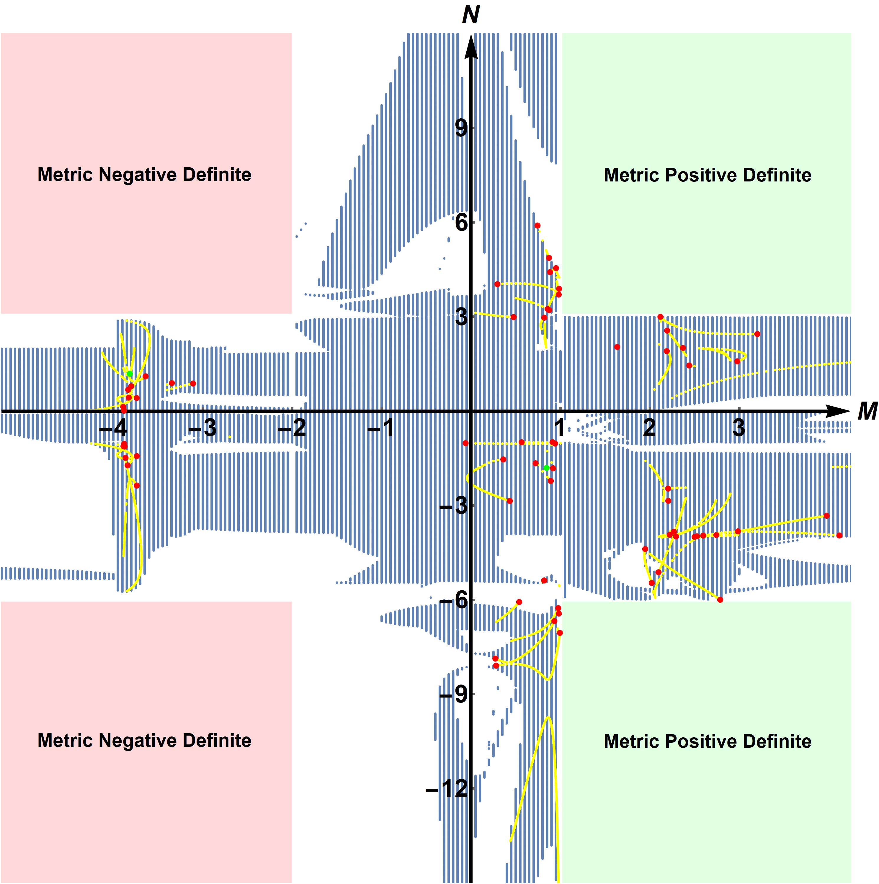
Figure 1: Bifurcation diagram in the space of $M$ and $N$. Spooky fixed points are present in the areas coloured in blue. Curves in yellow signify Andronov-Hopf bifurcations. Points coloured in red mark the locations of Bogdanov-Takens bifurcations, and points in green indicate Zero-Hopf bifurcations.

III Bogdanov-Takens Bifurcation

A Bogdanov-Takens bifurcation occurs generically when, at a fixed point, two eigenvalues of the stability matrix $\left(\frac{\partial\beta_{i}}{\partial g_{j}}\right)$ tend to zero as two bifurcation parameters $M$ and $N$ are appropriately tuned. The following equations must then be satisfied:

$$\beta_{i}(g_{i},N,M)=0\,,\quad\det\left(\frac{\partial\beta_{i}}{\partial g_{j}}\right)\left(g_{i},N,M\right)=0\,,$$ (5)

$$\operatorname{tr}\left[\textstyle\bigwedge^{3}\left(\frac{\partial\beta_{i}}{\partial g_{j}}\right)\right]\equiv\det\left(\frac{\partial\beta_{i}}{\partial g_{j}}\right)\operatorname{tr}\left[\left(\frac{\partial\beta_{i}}{\partial g_{j}}\right)^{-1}\right]=0\,.$$

Written in the form (5), we see that the conditions for a BT bifurcation are polynomial equations in $g_{i}$, $M$, and $N$, and so by Bézout’s theorem there exist at most a finite number of points that satisfy these conditions. We refer to such points as Bogdanov-Takens (BT) points. For the QFT we are studying perturbatively, it can be verified that the beta functions exhibit several such points, as shown in figure 1. Their existence can be checked to high numerical accuracy with the use of standard programs, e.g. PyDSTool pyd . Higher-loop contributions will provide corrections to the precise locations of these points, but as long as we take $\epsilon$ to be sufficiently small, higher-order corrections will not alter the number or qualitative behaviour of BT points.

While two eigenvalues tend to zero as we approach a BT point, right at the BT point itself we do not typically have a pair of eigenvectors with zero eigenvalues, the reason being that in this same limit, the two respective eigenvectors usually become linearly dependent. Rather, the stability matrix at a BT point has a Jordan block of size two with zero eigenvalue (see (9) in appendix A). This means that the theory at the BT point possesses two operators $\mathcal{O}_{1,2}$ such that the generator $D$ of dilatations acts in the following way

$$D\mathcal{O}_{1}=d\mathcal{O}_{1}\,,\quad D\mathcal{O}_{2}=d\mathcal{O}_{2}+\mathcal{O}_{1}\,.$$ (6)

The possibility of indecomposable representations of the conformal group was extensively studied in Gurarie (1993); Hogervorst et al. (2017). The upshot is that the BT theory constitutes a logarithmic CFT containing generalized marginal operators $\mathcal{O}_{1,2}$. In consequence, BT theories are non-unitary and we have

$$\braket{\mathcal{O}_{2}(0)\mathcal{O}_{2}(x)}=-\frac{2k_{\mathcal{O}}\log\left|x\right|}{\left|x\right|^{2d}}\,,\quad\braket{\mathcal{O}_{1}(0)\mathcal{O}_{2}(x)}=\frac{k_{\mathcal{O}}}{\left|x\right|^{2d}}\,,$$

for some constant $k_{\mathcal{O}}$.

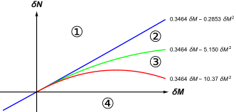
Figure 2: Bifurcation diagram around the Bogdanov-Takens bifurcation at $(M,N)=(M^{\ast},N^{\ast})\approx(0.2945,4.036)$. $\delta M=M-M^{\ast}$, $\delta N=N-N^{\ast}$. The blue curve represents a saddle node bifurcation, the green curve represents a Hopf bifurcation, and the red curve represents a saddle homoclinic bifurcation. At the origin, these three codimension-one bifurcations coalesce.

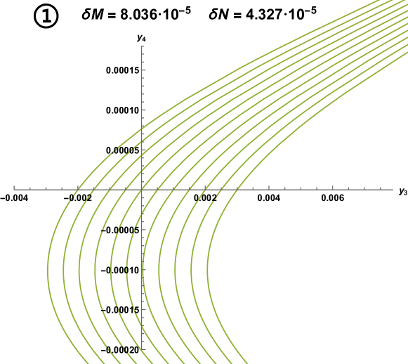
RG flow in region \raisebox{-.9pt} {1}⃝. In this regime, there are no fixed points near the origin, and all flow curves swerve downwards in the IR.

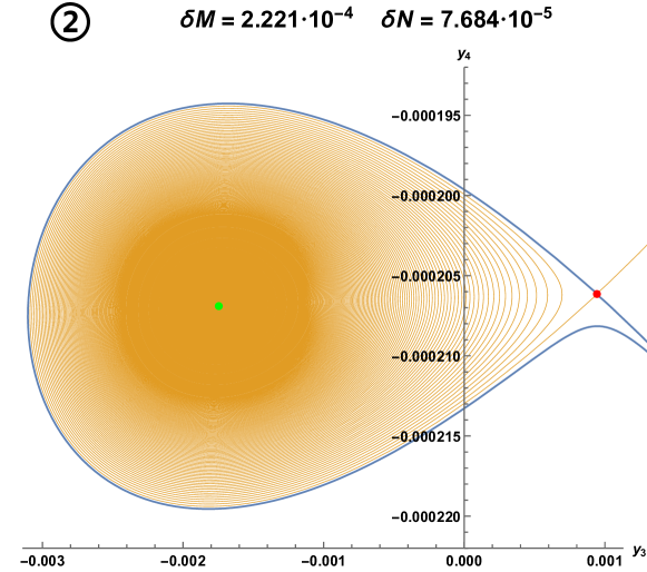
RG flow in region \raisebox{-.9pt} {2}⃝. The fixed point marked in red is a saddle point. The blue curves flow outwards from this point in the IR, while the orange curves flow inward. The fixed point marked in green is IR unstable.

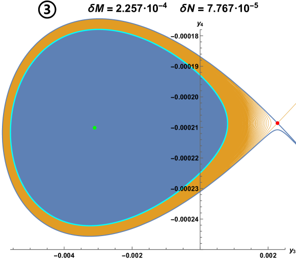
RG flow in region \raisebox{-.9pt} {3}⃝. In passing from region \raisebox{-.9pt} {2}⃝ to \raisebox{-.9pt} {3}⃝, the fixed point marked in green has undergone a Hopf bifurcation and is now IR stable. An IR-repulsive limit cycle, marked in cyan, separates the two fixed points.

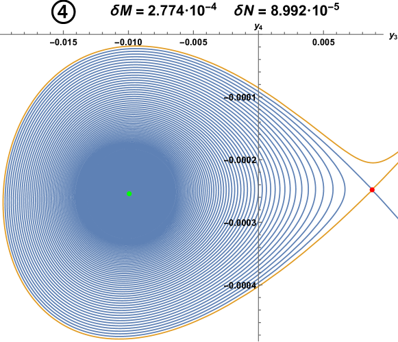
RG flow in region \raisebox{-.9pt} {4}⃝. In passing from region \raisebox{-.9pt} {3}⃝ to \raisebox{-.9pt} {4}⃝ the limit cycle collided with the red fixed point in a homoclinic bifurcation.

Figure 3: The topologically distinct types of RG flow in the vicinity of the Bogdanov-Takens bifurcation at $M=M^{\ast}\approx 0.2945$ and $N=N^{\ast}\approx 4.036$. The variables $y_{3}$ and $y_{4}$ are linear combinations of the four coupling constants $g_{i}$, with precise definitions given in appendix (A), and $\delta M=M-M^{\ast}$, $\delta N=N-N^{\ast}$.

The conditions (5) are not entirely sufficient to guarantee a BT bifurcation. One must also require smoothness and a set of inequalities that are generically true. Violations of the inequalities typically require fine-tuning of additional parameters and signal bifurcations of codimension higher than two. Incidentally, at the integer values $M=2$ and $N=3$, right on the boundary of the regimes with monotonic and non-monotonic RG flows, we observe a fixed point that satisfies (5), but which fails to meet these genericity requirements and for this reason is not described by a logarithmic CFT.

In appendix A we give the precise statement of the Bogdanov-Takens bifurcation theorem, and we explicitly check that it applies to an example of a BT point in the QFT we are studying, situated at $M\approx 0.2945$ and $N\approx 4.036$. What this means is that we can transform the beta functions near the BT point into a particularly simple form, known as Bogdanov normal form:

$$\left\{\begin{matrix}[l]\dot{\eta}_{1}=\eta_{2}\,,\\ \dot{\eta}_{2}=\delta_{1}+\delta_{2}\eta_{1}+\eta_{1}^{2}+s\eta_{1}\eta_{2}+\mathcal{O}\left(\left|\eta\right|^{3}\right)\,,\\ \dot{\eta}_{i}=\lambda_{i}\eta_{i}\quad\text{for }i>2\,,\end{matrix}\right.$$ (7)

where $s=-1$, and $\delta_{1,2}$ are functions of $N$ and $M$ that vanish right at the BT point.

By bringing the system into normal form, we can use the equations (7) to determine the behaviour of the system for small enough $\delta_{1}$ and $\delta_{2}$. In particular, we can constrain ourselves to studying the surface where only $\eta_{1}$ and $\eta_{2}$ are non-zero, noting that the dynamics in the transverse directions $\eta_{3}$ and $\eta_{4}$ are quite simple. Depending on the values of $\delta_{1}$ and $\delta_{2}$, the flow of $\eta_{1,2}$ falls into different topological types. The classification can be found in textbook Kuznetsov (2013) and amounts to the following. In the vicinity of the BT point at $\delta_{1}=\delta_{2}=0$, there are four regimes with qualitatively different flows:

– Regime \raisebox{-.9pt} {1}⃝: The flow has no fixed point.

In the other three regimes, the flow has two fixed-points, which we will label left and right. The right point is always a saddle point.

– Region \raisebox{-.9pt} {2}⃝: The left point is unstable, and all flow lines starting near it terminate at the right fixed point.

– Region \raisebox{-.9pt} {3}⃝: The left point is now stable, and a repulsive limit cycle separates the two fixed points.

– Region \raisebox{-.9pt} {4}⃝: The left point is still stable, but the limit cycle has disappeared. Some flow lines starting near the right fixed point terminate at the left fixed point.

In the case of the BT point at $(M,N)\approx(0.2945,4.036)$, the locations of these four adjoining regimes, as computed in appendix (7), is shown in figure 2. And the RG flow in each regime is depicted in figure 3.

The four regimes are separated by different codimension-one bifurcations. Region \raisebox{-.9pt} {1}⃝ is demarcated from regions \raisebox{-.9pt} {2}⃝ and \raisebox{-.9pt} {4}⃝ by a saddle-node bifurcation happening at $\delta_{1}=\frac{1}{4}\delta_{2}^{2}$. Regions \raisebox{-.9pt} {2}⃝ and \raisebox{-.9pt} {3}⃝ are separated by an Andronov-Hopf bifurcation along the the half-curve $\delta_{1}=0$, $\delta_{2}<0$. And regions \raisebox{-.9pt} {3}⃝ and \raisebox{-.9pt} {4}⃝ are separated by a saddle homoclinic bifurcation along $\delta_{1}=-\frac{6}{25}\delta_{2}^{2}+\ldots,\,\delta_{2}<0$.

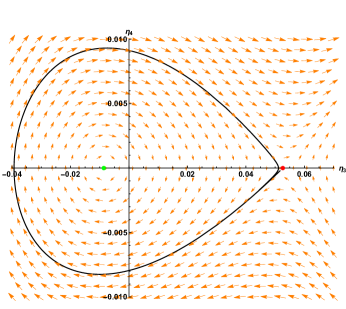
Figure 4: Flow diagram for a dynamical system containing a homoclinic orbit (marked in black), ie. a flow line that starts and ends at the same point. The system is described by equations (16) with parameters $\delta_{1}=-0.000453178$ and $\delta_{2}=-0.0440214$. The red and green dots indicate fixed points. The green dot is a ”spooky” fixed point. The theory at the red dot is a homoclinic CFT.

A saddle-node bifurcation corresponds to the collision and disappearance of two equilibria in dynamical systems. The phenomenon has been observed in a number of cases of RG flow, it happens for instance in in the critical $O(N)$ model Fei et al. (2015) and in prismatic models Giombi et al. (2018), and has been proposed to occur in $QCD_{4}$ Gies and Jaeckel (2006); Kaplan et al. (2009); Gorbenko et al. (2018a); Kuipers et al. (2019).

An Andronov-Hopf bifurcation represents a change of stability at a fixed point that has complex eigenvalues. The flow near the fixed point changes between spiraling inwards and spiraling outwards and gives birth to a limit cycle. In the context of RG, this bifurcation was recently studied in Jepsen et al. (2021).

The most interesting and new phenomenon associated to the model of the present paper happens along the homoclinic bifurcation line. Here the flow exhibits what is known as a homoclinic orbit.

IV Homoclinic RG flow

A homoclinic orbit is a flow line that connects a stable and an unstable direction of a saddle point. Figure (4) depicts the kind of homoclinic orbit generated by a BT bifurcation, with the saddle point marked by a red dot. The homoclinic orbit is seen to envelop another fixed point marked in green. In a QFT context, the green point is ”spooky”: the couplings are real, but the eigenvalues of the stability matrix $\left(\frac{\partial\beta_{i}}{\partial g_{j}}\right)$ have non-zero imaginary parts. In contrast to such spooky points, and to complex CFTs Gorbenko et al. (2018a, b), the red saddle point is associated to real couplings and real eigenvalues of the stability matrix. These eigenvalues are small and have opposite signs: $\lambda_{1},-\lambda_{2}\ll 1$. The positive eigenvalue corresponds to a slightly relevant operator $\mathcal{O}_{1}$ with dimension $\Delta_{1}=d+\lambda_{1}>d$, and the negative eigenvalue to a slightly irrelevant operator $\mathcal{O}_{2}$ with dimension $\Delta_{2}=d+\lambda_{2}<d$. In this sense, the red saddle point corresponds to a real CFT.

Standard RG lore states that if we perturb a system in the direction of a relevant operator, then we expect for the system to either lose conformality altogether or to flow to a different CFT. In the terminology of dynamical systems, standard RG trajectories are heteroclinic orbits. The classical example is the Wilson-Fischer fixed point: by carefully perturbing a Gaussian theory in $4-\epsilon$ dimension we flow to a weakly coupled interacting CFT, which in three dimensions interpolates to the Ising model. Homoclinic bifurcations provide exotic counterexamples to this general picture: if we perturb the system in the direction of a relevant operator, we come back to the original fixed point, which tentatively we can term a homoclinic CFT. Such RG behaviour obviously violates the $F$-theorem so that homoclinic fixed points must be non-unitary, as is generally the case for CFTs with symmetry groups of non-integer rank Binder and Rychkov (2020).

If we tune the bifurcation parameters so as to approach the BT point along the saddle homoclinic bifurcation (the red curve in figure 2), then the homoclinic orbit shrinks to a point and vanishes. In this limit, the red homoclinic CFT and the green spooky fixed point merge and become a logarithmic CFT.

V Zero-Hopf Bifurcations: The Road to Chaos

The Bogdanov-Takens bifurcation is not the only codimension-two bifurcation that can be observed to take place in the model (2). The theory also possesses two points in the space of $g_{i}$, $M$, and $N$ where the stability matrix has a pair of purely imaginary eigenvalues and one zero eigenvalue. Such fixed points indicate what is known as a Zero-Hopf (ZH) or a Fold-Hopf bifurcation. This type of bifurcation was classified in Takens (1974) and can be divided into six sub-types. In the notation of Guckenheimer and Holmes (2013), the model has a type I ZH bifurcation at $(M,N)\approx(0.8447,-1.807)$ and a type IIa ZH bifurcation at $(M,N)\approx(-3.816,1.188)$. At a type I bifurcation point, a saddle-node bifurcation is incident to a pitchfork bifurcation, and there are no nearby cyclic orbits. At a type IIa point, a saddle-node bifurcation is again incident to a pitchfork bifurcation, but additionally a Hopf bifurcation is also incident to the point, except that the stability coefficient of the associated limit cycle (what was referred to as the Hopf constant in Jepsen et al. (2021)) exactly vanishes in a quadratic approximation, so that cubic fluctuations or higher decide the fate of the cyclic flow near a type IIa point.

Generally, ZH bifurcation points are of particular interest because it is known that in their vicinity what is known as a Shilnikov homoclinic orbit may develop and render the system chaotic Kuznetsov (2013); Shilnikov (1965). Recently it was proven in Baldomá et al. (2020) that the presence of ZH bifurcations of type III guarantees the existence of a Shilnikov orbit and a nearby infinite set of saddle periodic orbits. This nontrivial invariant set can be embedded in an attracting domain, thus implying Shilnikov chaos.

The ZH points of the model in the present paper are not of type III, and we cannot claim that the system is chaotic. It may be worthwhile to investigate if there exist other models that meet the simple criteria for the assured appearance of chaos.

VI Conclusion and Outlook

The approach suggested and adopted in Gukov (2017); Kuipers et al. (2019); Jepsen et al. (2021) of studying the beta functions and renormalization of QFTs from the general perspective of dynamical systems provides a method of understanding the full range of possible RG flows. A powerful tool to this end is offered by Bogdanov’s and Taken’s bifurcation theorem Hopf (1942), which lists a simple set of conditions that guarantee the existence of a homoclinc RG orbit, and which can be checked already at first order in perturbation theory.

In this short letter we have presented a QFT that satisfies these conditions, namely a supersymmetric model with global symmetry group $O(N)\times O(M)$, where $N$ and $M$ play the role of the bifurcation parameters of the system. We determined a number of parameter values where a BT bifurcation takes place and investigated the nearby RG flow to uncover the presence of homoclinic orbits, where the perturbation of a fixed point by a relevant operator induces an RG flow that returns to its starting point along an irrelevant direction.

There are several bifurcation theorems that give simple criteria for other novel kinds of RG flows Guckenheimer and Holmes (2013); Kuznetsov (2013); Arnold (2012). Some of these theorems allow for the determination of the onset of chaotic flow based on straightforward computations around fixed points Baldomá et al. (2020). It would be interesting to find out if QFTs give birth to chaos when $N$ becomes fractional.

Appendix A Transformation to Normal Form

In this appendix we present a case study of one of the Bogdanov-Takens bifurcations present in the QFT with action (2).

At $M=M^{\ast}\approx 0.2945$ and $N=N^{\ast}\approx 4.036$, there exists an RG fixed point $g^{\ast}$ such that stability matrix

$$M_{i}{}^{j}=\left.\frac{\partial\beta_{i}}{\partial g_{j}}\right|_{g^{\ast}}$$ (8)

has a zero eigenvalue of multiplicity two in addition to two non-zero eigenvalues: $\lambda_{1}=2$ and $\lambda_{2}\approx-2.357$ (working in units of $\epsilon$). This implies the existence of a matrix $V=\big{(}\vec{v}_{1},\vec{v}_{2},\vec{v}_{3},\vec{v}_{4}\big{)}^{\intercal}$ such that

$$V^{-1}MV=\left(\begin{matrix}\lambda_{1}&0&0&0\\ 0&\lambda_{2}&0&0\\ 0&0&0&\lambda_{3}\\ 0&0&0&0\end{matrix}\right)$$ (9)

where $\vec{v}_{i}$ are (generalized) unit eigenvectors, and $\lambda_{3}\approx 7.555$ is a generalized eigenvalue. That is,

$$M\vec{v}_{1,2}=\lambda_{1,2}\vec{v}_{1,2}\,,\quad M\vec{v}_{3}=0\,,\quad M\vec{v}_{4}=\lambda_{3}\vec{v}_{3}\,.$$

By a change of variables from $\vec{g}$ to $\vec{h}=V^{-1}(\vec{g}-\vec{g}^{\ast})$, we obtain differential equations where $h_{1}$ and $h_{2}$ do not mix linearly with $h_{3}$ and $h_{4}$:

$$\beta_{h_{1,2}}=\lambda_{1,2}h_{1,2}+\mathcal{O}(h^{2})\,.$$ (10)

Consider now the case when $M=M^{\ast}+\delta M$ and $N=N^{\ast}+\delta M$, where $\delta M$ and $\delta N$ are each suppressed by a small parameter $\alpha\ll 1$. That is, $\delta M,\delta N\sim\alpha$. If we adopt the $h$ variables, $h_{1}$ and $h_{2}$ will now mix linearly with each other and with $h_{3}$ and $h_{4}$, and their beta functions will contain constant terms. We can write

$$\frac{dh_{1}}{dt}=B_{0,1}+A_{1,1}h_{1}+B_{1,2}h_{2}+B_{1,3}h_{3}+B_{1,4}h_{4}+\mathcal{O}(h^{2})$$

$$\frac{dh_{2}}{dt}=B_{0,0}+B_{2,1}h_{1}+A_{2,2}h_{2}+B_{2,3}h_{3}+B_{2,4}h_{4}+\mathcal{O}(h^{2})\,,$$

for some coefficients $A_{i,j}$ and $B_{i,j}$, where the coefficients $B_{i,j}$ are all suppressed in $\alpha$. Introducing new variables

$$y_{1}=h_{1}+C_{1,0}+C_{1,3}h_{3}+C_{1,4}h_{4}\,,$$

$$y_{2}=h_{2}+C_{2,0}+C_{2,3}h_{3}+C_{2,4}h_{4}\,,$$ (11)

we can choose the six coefficients $C_{i,j}$ such that $\frac{dy_{1,2}}{dt}$ do not contain constant terms nor mix linearly with $h_{3}$ and $h_{4}$. This means that, studying only the RG flow near the origin so that cubic terms and higher can be disregarded, the surface $y_{1}=y_{2}=0$ is an invariant manifold. On this surface, we can define variables $y_{3}=h_{3}$ and $y_{4}=\lambda_{3}h_{4}$, whose RG flow to quadratic order in the dynamic variables is governed by the differential equations

$$\frac{dy_{3}}{dt}=a_{00}+a_{10}y_{3}+a_{01}y_{4}+\frac{1}{2}a_{20}y_{3}^{2}+a_{11}y_{3}y_{4}+\frac{1}{2}a_{02}y_{4}^{2}\,,$$ (12)

$$\frac{dy_{4}}{dt}=b_{00}+b_{10}y_{3}+b_{01}y_{4}+\frac{1}{2}b_{20}y_{3}^{2}+b_{11}y_{3}y_{4}+\frac{1}{2}b_{02}y_{4}^{2}\,.$$

For the specific BT point we are considering, omitting higher order terms in $\alpha$, the values of the various coefficients are given by

$$a_{00}=\,12.75\,\delta N+2.618\,\delta M\,,$$

$$a_{10}=\,46.93\,\delta N-8.164\,\delta M\,,$$

$$a_{01}=\,1\,,\quad a_{20}=\,0.6040\,,$$

$$a_{11}=\,-2.268\,,\quad a_{02}=\,-0.9708\,,$$

$$b_{00}=\,19.49\,\delta N-6.753\,\delta M-638.9\,\delta N^{2}$$

$$+99.89\,\delta M^{2}-71.61\,\delta N\,\delta M\,,$$

$$b_{10}=\,-51.76\,\delta N+17.38\,\delta M\,,$$

$$b_{01}=\,-18.05\,\delta N-0.4165\,\delta M\,,$$

$$b_{20}=\,2.775\,,\quad b_{11}=\,-0.7935\,,\quad b_{02}=\,-1.868\,.$$ (13)

We now restrict attention to the case when $\delta N$ and $\delta M$ are tuned such that $b_{00}\sim\alpha^{2}$, for the reason that this will turn out to be the regime where the existence of a homoclinic orbit can be reliably established. Working merely to leading order in $\alpha$ and to quadratic order in the dynamical variables, we perform a reparametrization from $t$ to $\tau$ via

$$d\tau= -\frac{1}{2}\frac{b_{20}}{a_{20}+b_{11}}\Big{(}1-\frac{2a_{11}+b_{02}}{2}\,\frac{dy_{3}}{dt}\Big{)}^{-1}dt$$ (14)

and change to variables $\eta_{1}$ and $\eta_{2}$ given by

$$\eta_{1}=2\frac{a_{20}+b_{11}}{b_{20}}\Big{(}(a_{20}+b_{11})y_{3}+a_{01}+b_{01}-a_{00}a_{11}-a_{00}b_{02}\Big{)}$$

$$\eta_{2}=-4\frac{(a_{20}+b_{11})^{3}}{b_{20}^{2}}\times$$ (15)

$$\times\bigg{(}1-\frac{2a_{11}+b_{02}}{2}\Big{(}y_{3}+\frac{a_{10}b_{01}-a_{00}a_{11}-a_{00}b_{02}}{a_{20}+b_{11}}\Big{)}\bigg{)}\frac{dy_{3}}{dt}\,,$$

where for $\frac{dy_{3}}{dt}$ one should substitute the RHS of (12). In these new variables, the differential equations of the dynamical system are brought into the normal form introduced by Bogdanov:

$$\left\{\begin{matrix}[l]\dot{\eta}_{3}=\eta_{4}\,,\\ \dot{\eta}_{4}=\delta_{1}+\delta_{2}\eta_{3}+\eta_{3}^{2}+\eta_{3}\eta_{4}\,,\\ \end{matrix}\right.$$ (16)

where we have omitted terms of cubic order and higher in $\eta$, and the parameters $\delta_{1}$ and $\delta_{2}$ are given by

$$\delta_{1}=\frac{8(a_{20}+b_{11})^{4}}{b_{20}^{3}}\bigg{(}b_{00}-a_{00}b_{01}+\frac{a_{00}^{2}b_{02}}{2}+\frac{\big{(}a_{10}+b_{01}-a_{00}(a_{11}+b_{02})\big{)}(a_{00}b_{11}-b_{10})}{a_{20}+b_{11}}+\frac{\big{(}a_{10}+b_{01}-a_{00}(a_{11}+b_{02})\big{)}^{2}b_{20}}{2(a_{20}+b_{11})^{2}}\bigg{)}\,,$$

$$\delta_{2}=\frac{4(a_{20}+b_{11})}{b_{20}^{2}}\bigg{(}(a_{20}+b_{11})(b_{10}-a_{00}b_{11})-\big{(}a_{10}+b_{01}-a_{00}(a_{11}+b_{02})\big{)}b_{20}\bigg{)}\,.$$ (17)

The transformations by which we arrived at the equations (16) can be applied more generally to dynamical systems where the stability matrix contains a Jordan block with zero eigenvalues, as long as the following conditions are met:

$$\lambda_{3}\neq 0\,,\quad b_{20}\neq 0\,,\quad a_{20}+b_{11}\neq 0\,.$$ (18)

This fact is known as the Bogdanov-Takens bifurcation theorem Bogdanov (1981); Takens (2001); MR2197746; MR3501359. The precise formulation of the theorem is this:

Theorem.

Suppose we have a system of differential equations

$$\dot{\vec{x}}=\vec{f}(\vec{x},\vec{\alpha}),\quad\vec{x}\in\mathbb{R}^{n},\,\vec{\alpha}\in\mathbb{R}^{2},$$ (19)

where $\vec{f}$ is smooth, and suppose further that $\vec{f}(0,0)=0$ and that the stabililty matrix $\left(\frac{\partial\vec{f}}{\partial\vec{x}}\right)\Big{|}_{\vec{x}=\vec{\alpha}=0}$ has a Jordan cell of size two with zero eigenvalues: $\lambda_{1,2}=0$ and other eigenvalues $\lambda_{3},\ldots,\lambda_{n}$ with non-zero real parts. Assume that the map $\left(\vec{x},\vec{\alpha}\right)\longmapsto\left(\vec{f}(\vec{x},\vec{\alpha}),\operatorname{tr}\left(\frac{\partial f_{i}}{\partial x_{j}}\right),\det\left(\frac{\partial f_{i}}{\partial x_{j}}\right)\right)$ is smooth and that the non-degeneracy conditions (18) are satisfied. Then there exists a smooth invertible variable transformation, a direction-preserving time reparametrization, and a smooth invertible change of parameters that together reduce the system to the normal form (7), where $\delta_{1,2}$ are functions of $\vec{\alpha}$ and $s=\pm 1$.

Furthermore, there is a theorem stating that the suppressed terms of cubic order and higher in (7) do not change the local topology of the flow. But the topology of the flow of the normal form system, omitting cubic and higher terms, is well understood. In particular, it is known that depending on the values of $\delta_{1}$ and $\delta_{2}$, the flow near the origin can be divided into four distinct regions. As described in section III, these four regions are separated by codimension-one bifurcations located on the curve $\delta_{1}=\frac{1}{4}\delta_{2}^{2}$ and, for $\delta_{2}<0$, on the curves $\delta_{1}=0$ and $\delta_{1}=-\frac{6}{25}\delta_{2}^{2}$. For the specific BT point at $M\approx 2.945$ and $N\approx 4.036$, we can translate these equations into relations between $\delta M$ and $\delta N$, whereby we arrive at the picture of figure 2.

As mentioned in section II, there is a fixed point at $M=2$, $N=3$, which does have a stability matrix with a zero eigenvalue of multiplicity two, but which does not meet the genericity conditions (18). Because the point is situated at the value $N=3$, the metric is degenerate, and only three of the four operators (1) are linearly dependent. Specifically,

$$2O_{1}+4O_{2}-2O_{3}-O_{1}\,\big{|}_{N=3}=0\,.$$ (20)

It turns out that the operator $\mathcal{O}_{2}$ corresponding to the eigenvalue $\lambda_{2}$ is identically zero owing to this linear relationship, so that the space of couplings is three-dimensional, and the stability matrix at the fixed point has eigenvalues $2$, $0$, and $0$. But the fixed point is not described by a logarithmic CFT, nor does it represent a BT bifurcation, the reason being that the generalized eigenvalue $\lambda_{3}$ is zero.

Appendix B Two-Loop Beta Functions

The beta functions of the four coupling constants admit loop expansions

$$\beta_{i}=-\epsilon g_{i}+\beta_{i}^{(2)}+\mathcal{O}(g^{5})\,,$$ (21)

where $\beta_{i}^{(2)}$ denotes the two-loop contributions, which are cubic in the couplings. By explicit computation using Popov (2020), we find that these are given by

$$\beta_{1}^{(2)}=\, \frac{1}{8\pi^{2}N^{2}}\bigg{(}32g_{1}^{2}g_{4}N(-40-8M+8N+7MN+8N^{2})+16g_{1}^{2}g_{3}N(-80-24M+30N+4MN+7N^{2}+4MN^{2})$$

$$+16g_{1}g_{3}^{2}N^{2}(32+2M+N+MN+N^{2}+MN^{2})+64g_{1}g_{2}g_{4}N(-32-4M+16N+2MN+5N^{2}+2MN^{2})$$

$$+4g_{2}^{2}g_{3}N(-256-64M+72N+10MN+19N^{2}+2MN^{2})+64g_{1}g_{4}^{2}N^{2}(22-2M+MN+MN^{2})$$

$$+16g_{1}g_{2}g_{3}N(-144-40M+42N+17MN+21N^{2}+5MN^{2})+128g_{1}g_{3}g_{4}N^{2}(3+5M+N+N^{2})$$

$$+g_{2}^{3}(896+128M-352N-48MN-12N^{2}-12MN^{2}+7N^{3}+2MN^{3})+96g_{2}^{2}g_{4}(-8+N)N$$ (22)

$$+4g_{1}^{2}g_{2}(928+224M-392N-100MN-2N^{2}+11MN^{2}+23N^{3}+7MN^{3}+4N^{4})+768g_{2}g_{3}g_{4}N^{2}$$

$$+4g_{1}^{3}(352+96M-152N-44MN+10N^{3}+3MN^{3}+MN^{4})+16g_{2}g_{3}^{2}N^{2}(16+7M+N+N^{2})$$

$$+2g_{1}g_{2}^{2}(1600+320M-656N-136MN+32N^{2}+10MN^{2}+50N^{3}+10MN^{3}+5N^{4}+2MN^{4})\bigg{)}\,,$$

$$\beta_{2}^{(2)}=\, \frac{1}{8\pi^{2}N^{2}}\bigg{(}64g_{1}g_{2}g_{4}N(-80-16M+16N+5MN+7N^{2})+16g_{2}g_{3}^{2}N^{2}(48+9M+2N+MN+2N^{2}+MN^{2})$$

$$+16g_{1}^{2}g_{3}N(-128-32M+32N+12MN+14N^{2}+3MN^{2})+128g_{2}g_{3}g_{4}N^{2}(9+5M+N+N^{2})$$

$$+16g_{1}g_{2}g_{3}N(-272-72M+82N+15MN+24N^{2}+6MN^{2})+192g_{1}^{2}g_{4}N(-12-2M+4N+N^{2})$$ (23)

$$+16g_{2}^{2}g_{4}N(-176-40M+58N+14MN+17N^{2}+11MN^{2})+32g_{1}g_{3}^{2}N^{2}(16+7M+N+N^{2})$$

$$+4g_{2}^{2}g_{3}N(-576-160M+176N+54MN+74N^{2}+17MN^{2})+64g_{2}g_{4}^{2}N^{2}(22-2M+MN+MN^{2})$$

$$+8g_{1}^{3}(288+64M-112N-24MN-6N^{2}+3MN^{2}+5N^{3}+2MN^{3}+N^{4})+1536g_{1}g_{3}g_{4}N^{2}$$

$$+2g_{1}g_{2}^{2}(3968+1024M-1600N-416MN-56N^{2}-22MN^{2}+85N^{3}+17MN^{3}+11N^{4})$$

$$+4g_{1}^{2}g_{2}(1856+448M-736N-176MN-22N^{2}-5MN^{2}+43N^{3}+8MN^{3}+3N^{4}+2MN^{4})$$

$$+g_{2}^{3}(2816+768M-1152N-320MN+12N^{2}-12MN^{2}+69N^{3}+30MN^{3}+7N^{4}+5MN^{4})\bigg{)}\,,$$

$$\beta_{3}^{(2)}=\, \frac{1}{8\pi^{2}N^{3}}\bigg{(}32g_{3}^{2}g_{4}N^{3}(18+14M+7N+7N^{2})+96g_{1}^{2}g_{4}N(8+2N^{2}+MN^{2})+384g_{1}g_{2}g_{4}N(4+N^{2})$$

$$+24g_{3}^{3}N^{3}(16+2M+2N+MN+2N^{2}+MN^{2})+64g_{2}g_{3}g_{4}N^{2}(-20-4M+10N+2MN+5N^{2}+2MN^{2})$$

$$+16g_{1}g_{3}^{2}N^{2}(-52-14M+26N+7MN+14N^{2}+7MN^{2})+128g_{1}g_{3}g_{4}N^{2}(-10-2M+5N+MN+5N^{2})$$

$$+8g_{2}g_{3}^{2}N^{2}(-104-28M+52N+14MN+38N^{2}+7MN^{2})+64g_{3}g_{4}^{2}N^{3}(22-2M+MN+MN^{2})$$

$$+16g_{1}g_{2}g_{3}N(208+56M-48N-12MN+12N^{2}+3MN^{2}+8N^{3}+MN^{3}+2N^{4})+96g_{2}^{2}g4N(8+N^{2})$$

$$+8g_{1}^{2}g_{3}N(208+56M-48N-12MN+12N^{2}+6MN^{2}+4N^{3}+3MN^{3}+MN^{4})$$ (24)

$$+8g_{1}^{3}(-96-16M+24N+4MN-20N^{2}-10MN^{2}+6N^{3}+2MN^{3}+N^{4}+MN^{4})$$

$$+4g_{2}^{2}g_{3}N(416+112M-96N-24MN+18N^{2}+6MN^{2}+12N^{3}+4MN^{3}+2N^{4}+MN^{4})$$

$$+g_{2}^{3}(-768-128M+192N+32MN-96N^{2}+32N^{3}+4MN^{3}+7N^{4}+2MN^{4})$$

$$+2g_{1}g_{2}^{2}(-1152-192M+288N+48MN-176N^{2}-40MN^{2}+70N^{3}+10MN^{3}+21N^{4}+2MN^{4})$$

$$+4g_{1}^{2}g_{2}(-576-96M+144N+24MN-104N^{2}-40MN^{2}+34N^{3}+13MN^{3}+11N^{4}+3MN^{4})\bigg{)}\,,$$

$$\beta_{4}^{(2)}=\, \frac{1}{8\pi^{2}N^{3}}\bigg{(}8g_{1}^{2}g_{3}N(80+16M-12N+4N^{2}+2MN^{2}+3N^{3}+N^{4})$$

$$+224g_{1}g_{4}^{2}N^{2}(-4-2M+2N+MN+2N^{2})+16g_{1}g_{3}^{2}N^{2}(-16-2M+8N+MN+7N^{2})$$

$$+96g_{4}^{3}N^{3}(8-2M+MN+MN^{2})+64g_{2}g_{3}g_{4}N^{2}(-14-4M+7N+2MN+6N^{2}+MN^{2})$$

$$+224g_{2}g_{4}^{2}N^{2}(-4-2M+2N+MN+N^{2}+MN^{2})+32g_{3}^{2}g_{4}N^{3}(22+N+MN+N^{2}+MN^{2})$$

$$+64g_{1}g_{3}g_{4}N^{2}(-14-4M+7N+2MN+2N^{2}+2MN^{2})$$

$$+8g_{2}g_{3}^{2}N^{2}(-32-4M+16N+2MN+9N^{2}+2MN^{2})+24g_{3}^{3}N^{3}(4+2M+N+N^{2})$$

$$+16g_{1}g_{2}g_{3}N(80+16M-12N+7N^{2}+2MN^{2}+N^{3})+224g_{3}g_{4}^{2}N^{3}(2M+N+N^{2})$$

$$+4g_{2}^{2}g_{3}N(160+32M-24N+17N^{2}+7MN^{2}+4N^{3}+N^{4})$$

$$+32g_{1}g_{2}g_{4}N(96+36M-24N-12MN+2N^{2}-2MN^{2}+4N^{3}+MN^{3}+N^{4})$$

$$+4g_{1}^{3}(-160-48M+40N+12MN+4N^{2}+2MN^{2}+4N^{3}+MN^{3}+2N^{4})$$

$$+2g_{1}g_{2}^{2}(-960-288M+240N+72MN-88N^{2}-20MN^{2}+39N^{3}+7MN^{3}+13N^{4})$$

$$+16g_{1}^{2}g_{4}N(96+36M-24N-12MN-4N^{2}-2MN^{2}+2N^{3}+3MN^{3}+MN^{4})$$

$$+8g_{1}^{2}g_{2}(-240-72M+60N+18MN-8N^{2}-MN^{2}+6N^{3}+2MN^{3}+N^{4}+MN^{4})$$

$$+8g_{2}^{2}g_{4}N(192+72M-48N-24MN+10N^{2}+2MN^{2}+6N^{3}+4MN^{3}+N^{4}+MN^{4})$$

$$+g_{2}^{3}(-640-192M+160N+48MN-96N^{2}-24MN^{2}+36N^{3}+12MN^{3}+10N^{4}+5MN^{4})\bigg{)}\,.$$

By proper rescaling $g_{i}\to\epsilon\tilde{g_{i}}$ we can get rid of $\epsilon$ in the equation (21). It can be checked that there exists a function $F$ of the couplings such that the beta-functions (B)-(B) can be cast in the form

$$\beta_{i}=G_{ij}\frac{\partial F}{\partial g_{j}}$$ (25)

where the metric has the components

$$G_{11}= \frac{MN^{4}+3MN^{3}+2N^{3}-2MN^{2}-4N^{2}-12MN-24N+24M+48}{2N^{2}}\,,$$

$$G_{12}= \frac{N^{4}+MN^{3}+4N^{3}-2MN^{2}-4N^{2}-12MN-24N+24M+48}{2N^{2}}\,,$$

$$G_{13}= 2\,\frac{MN^{2}+N^{2}+MN+2N-2M-4}{N}\,,\quad G_{14}=2\,\frac{2N^{2}+MN+2N-2M-4}{N}\,,$$

$$G_{22}= \frac{MN^{4}+N^{4}+4MN^{3}+6N^{3}-4MN^{2}-8N^{2}-24MN-48N+48M+96}{4N^{2}}\,,$$

$$G_{23}= \frac{MN^{2}+3N^{2}+2MN+4N-4M-8}{N}\,,\quad G_{24}=2\frac{MN^{2}+N^{2}+MN+2N-2M-4}{N}\,,$$

$$G_{33}= \frac{MN^{3}+N^{3}+MN^{2}+N^{2}+4N}{N}\,,\quad G_{34}=2(N^{2}+N+2M)\,,\quad G_{44}=2(4-2M+MN+MN^{2})\,.$$

Taking the determinant of this metric, one arrives at (4).

Appendix C Bifurcation Conditions

When working to two-loop level, the beta functions have the property that $\beta_{i}+\epsilon g_{i}$ is a homogeneous function of degree three. Hence, by Euler’s theorem,

$$g_{j}\frac{\partial(\beta_{i}+\epsilon g_{i})}{\partial g_{j}}=3(\beta_{i}+\epsilon g_{i})\,.$$ (26)

By evaluating this equation on an RG fixed point $\vec{g}^{*}$, one finds that

$$\left.M_{j}{}^{i}\right|_{\vec{g}=\vec{g}^{*}}g^{*}_{i}=2\epsilon g_{j}^{*}\,,$$ (27)

where $M_{j}{}^{i}=\frac{\partial\beta_{j}}{\partial g_{i}}$ is the stability matrix defined in (8). Hence, for any non-trivial fixed point, the stability matrix has an eigenvalue $\lambda_{1}=2\epsilon$ equal to two. This fact allows for simplifications in the conditions for bifurcations to occur.

Consider the determinant $\det\left(M-\lambda\right)$. Since it is a fourth order polynomial in $\lambda$, we can write

$$\det\left(M-\lambda\right)=\lambda^{4}+A\lambda^{3}+B\lambda^{2}+C\lambda+D\,,$$ (28)

where $A$, $B$, $C$, and $D$ are $M$- and $N$-dependent polynomials in the coupling constants. Specifially

$$A=-\text{Tr}M\,,\quad B=M_{ij,ij}\,,\quad C=-M_{i,i}\,,\quad D=\det M\,,$$

where $M_{i,j}$ and $M_{ij,kl}$ are the first and second minors of the stability matrix. But when evaluated on a fixed point, we also have the following factorization in terms of eigenvalues (in units where $\epsilon=1$)

$$\det\left(M_{\ast}-\lambda\right)=(\lambda-2)(\lambda-\lambda_{2})(\lambda-\lambda_{3})(\lambda-\lambda_{4})\,.$$

By expanding out the factors on the RHS, we can relate $A$, $B$, and $C$ to the eigenvalues.

A saddle-node bifurcation occurs when at a fixed point we have a zero-eigenvalue: $\lambda_{2}=0$. In this case, one finds that

$$A=-2-\lambda_{3}-\lambda_{4}\,,\hskip 14.22636ptB=2(\lambda_{3}+\lambda_{4})+\lambda_{3}\lambda_{4}\,,$$

$$C=-2\lambda_{3}\lambda_{4}\,,$$ (29)

from which one can derive the equation

$$2B+C=-4(A+2)\,.$$ (30)

Of course we also have the equation $D=0$, but the condition (30) is easier to check numerically on account of the many terms in the determinant.

At a Hopf bifurcation, we have a conjugate pair of imaginary eigenvalues:

$$\lambda_{3}=i\chi\,,\hskip 17.07164pt\lambda_{4}=-i\chi\,,$$ (31)

where $\chi$ is a real number. Consequently we find that

$$A=-2-\lambda_{2}\,,\hskip 10.5275ptB-2\lambda_{2}+\chi^{2}\,,\hskip 10.5275ptC=-(2+\lambda_{2})\chi^{2}\,.$$

From these equations, we derive the condition

$$C=A(B+4+2A)\,.$$ (32)

At a Bogdanov-Takens bifurcation, there are two zero eigenvalues: $\lambda_{3}=\lambda_{4}=0$. From this, one obtains the conditions

$$B=-2(A+2)\,,\hskip 22.76219ptC=0\,.$$ (33)

We have a Zero-Hopf bifurcation when

$$\lambda_{2}=0\,,\hskip 14.22636pt\lambda_{3}=i\chi\,,\hskip 14.22636pt\lambda_{4}=-i\chi\,,$$ (34)

with $\chi$ a real number. In this case

$$A=-2\,,\hskip 22.76219ptC=-2B\,.$$ (35)

References

- Wilson and Kogut (1974) K.G. Wilson and John B. Kogut, “The Renormalization group and the epsilon expansion,” Phys. Rept. 12, 75–199 (1974).
- Guckenheimer and Holmes (2013) John Guckenheimer and Philip Holmes, Nonlinear oscillations, dynamical systems, and bifurcations of vector fields, Vol. 42 (Springer Science & Business Media, 2013).
- Arnold (2012) Vladimir Igorevich Arnold, Geometrical methods in the theory of ordinary differential equations, Vol. 250 (Springer Science & Business Media, 2012).
- Gukov (2017) Sergei Gukov, “RG Flows and Bifurcations,” Nucl. Phys. B 919, 583–638 (2017), arXiv:1608.06638 [hep-th] .
- Feigenbaum (1978) Mitchell J Feigenbaum, “Quantitative universality for a class of nonlinear transformations,” Journal of statistical physics 19, 25–52 (1978).
- Zamolodchikov (1986) Alexander B Zamolodchikov, “Irreversibility of the flux of the renormalization group in a 2d field theory,” JETP lett 43, 730–732 (1986).
- Komargodski and Schwimmer (2011) Zohar Komargodski and Adam Schwimmer, “On Renormalization Group Flows in Four Dimensions,” JHEP 12, 099 (2011), arXiv:1107.3987 [hep-th] .
- Luty et al. (2013) Markus A. Luty, Joseph Polchinski, and Riccardo Rattazzi, “The -theorem and the Asymptotics of 4D Quantum Field Theory,” JHEP 01, 152 (2013), arXiv:1204.5221 [hep-th] .
- Klebanov et al. (2011) Igor R. Klebanov, Silviu S. Pufu, and Benjamin R. Safdi, “F-Theorem without Supersymmetry,” JHEP 10, 038 (2011), arXiv:1105.4598 [hep-th] .
- Jafferis et al. (2011) Daniel L. Jafferis, Igor R. Klebanov, Silviu S. Pufu, and Benjamin R. Safdi, “Towards the F-Theorem: N=2 Field Theories on the Three-Sphere,” JHEP 06, 102 (2011), arXiv:1103.1181 [hep-th] .
- Casini and Huerta (2012) H. Casini and Marina Huerta, “On the RG running of the entanglement entropy of a circle,” Phys. Rev. D 85, 125016 (2012), arXiv:1202.5650 [hep-th] .
- Morozov and Niemi (2003) Alexei Morozov and Antti J Niemi, “Can renormalization group flow end in a big mess?” Nuclear Physics B 666, 311–336 (2003).
- Curtright et al. (2012) Thomas L. Curtright, Xiang Jin, and Cosmas K. Zachos, “RG flows, cycles, and c-theorem folklore,” Phys. Rev. Lett. 108, 131601 (2012), arXiv:1111.2649 [hep-th] .
- Bernard and LeClair (2001) Denis Bernard and Andre LeClair, “Strong weak coupling duality in anisotropic current interactions,” Phys. Lett. B 512, 78–84 (2001), arXiv:hep-th/0103096 .
- LeClair et al. (2004a) Andre LeClair, Jose Maria Roman, and German Sierra, “Log periodic behavior of finite size effects in field theories with RG limit cycles,” Nucl. Phys. B 700, 407–435 (2004a), arXiv:hep-th/0312141 .
- Leclair et al. (2003) Andre Leclair, Jose Maria Roman, and German Sierra, “Russian doll renormalization group, Kosterlitz-Thouless flows, and the cyclic sine-Gordon model,” Nucl. Phys. B 675, 584–606 (2003), arXiv:hep-th/0301042 .
- Glazek and Wilson (1993) Stanislaw D. Glazek and K. G. Wilson, “Renormalization of overlapping transverse divergences in a model light front Hamiltonian,” Phys. Rev. D 47, 4657–4669 (1993).
- Glazek and Wilson (2002) Stanislaw D. Glazek and Kenneth G. Wilson, “Limit cycles in quantum theories,” Phys. Rev. Lett. 89, 230401 (2002), [Erratum: Phys.Rev.Lett. 92, 139901 (2004)], arXiv:hep-th/0203088 .
- Bulycheva and Gorsky (2014) K. M. Bulycheva and A. S. Gorsky, “Limit cycles in renormalization group dynamics,” Phys. Usp. 57, 171–182 (2014), arXiv:1402.2431 [hep-th] .
- Gorsky and Popov (2014) Alexander Gorsky and Fedor Popov, “Atomic collapse in graphene and cyclic renormalization group flow,” Phys. Rev. D 89, 061702 (2014), arXiv:1312.7399 [cond-mat.mes-hall] .
- LeClair et al. (2004b) Andre LeClair, Jose Maria Roman, and German Sierra, “Russian doll renormalization group and superconductivity,” Phys. Rev. B 69, 020505 (2004b), arXiv:cond-mat/0211338 .
- Braaten and Phillips (2004) Eric Braaten and Demian Phillips, “The Renormalization group limit cycle for the 1/r**2 potential,” Phys. Rev. A 70, 052111 (2004), arXiv:hep-th/0403168 .
- Dawid et al. (2018) Sebastian M. Dawid, R. Gonsior, J. Kwapisz, K. Serafin, M. Tobolski, and S. D. Głazek, “Renormalization group procedure for potential ,” Phys. Lett. B 777, 260–264 (2018), arXiv:1704.08206 [quant-ph] .
- Jepsen et al. (2021) Christian B. Jepsen, Igor R. Klebanov, and Fedor K. Popov, “RG limit cycles and unconventional fixed points in perturbative QFT,” Phys. Rev. D 103, 046015 (2021), arXiv:2010.15133 [hep-th] .
- De Gennes and Gennes (1979) Pierre-Gilles De Gennes and Pierre-Gilles Gennes, Scaling concepts in polymer physics (Cornell university press, 1979).
- Binder and Rychkov (2020) Damon J. Binder and Slava Rychkov, “Deligne Categories in Lattice Models and Quantum Field Theory, or Making Sense of Symmetry with Non-integer ,” JHEP 04, 117 (2020), arXiv:1911.07895 [hep-th] .
- Hopf (1942) E Hopf, “Bifurcation of a periodic solution from a stationary solution of a system of differential equations,” Berlin Mathematische Physics Klasse, Sachsischen Akademic der Wissenschaften Leipzig 94, 3–32 (1942).
- Bogdanov (1981) Rifkat Bogdanov, “Bifurcations of a limit cycle for a family of vector fields on the plane.” Selecta Math. Soviet 1, 373–388 (1981).
- Takens (2001) Floris Takens, “Forced oscillations and bifurcations,” Applications of Global Analysis I, Comm 3, 1–62 (2001).
- Cvitanovic (2017) Predrag Cvitanovic, Universality in chaos (Routledge, 2017).
- Ruelle and Takens (1971) David Ruelle and Floris Takens, “On the nature of turbulence,” Les rencontres physiciens-mathématiciens de Strasbourg-RCP25 12, 1–44 (1971).
- Zakharov et al. (2012) Vladimir E Zakharov, Victor S L’vov, and Gregory Falkovich, Kolmogorov spectra of turbulence I: Wave turbulence (Springer Science & Business Media, 2012).
- Lorenz (1963) Edward N Lorenz, “Deterministic nonperiodic flow,” Journal of atmospheric sciences 20, 130–141 (1963).
- Gross and Rosenhaus (2021) David J. Gross and Vladimir Rosenhaus, “Chaotic scattering of highly excited strings,” (2021), arXiv:2103.15301 [hep-th] .
- Shilnikov (1965) Leonid Pavlovich Shilnikov, “A case of the existence of a denumerable set of periodic motions,” in Doklady Akademii Nauk, Vol. 160 (Russian Academy of Sciences, 1965) pp. 558–561.
- Oliynyk et al. (2006) T. Oliynyk, V. Suneeta, and E. Woolgar, “A Gradient flow for worldsheet nonlinear sigma models,” Nucl. Phys. B 739, 441–458 (2006), arXiv:hep-th/0510239 .
- Kuipers et al. (2019) Folkert Kuipers, Umut Gürsoy, and Yuri Kuznetsov, “Bifurcations in the RG-flow of QCD,” JHEP 07, 075 (2019), arXiv:1812.05179 [hep-th] .
- Collins (1986) John C. Collins, Renormalization: An Introduction to Renormalization, The Renormalization Group, and the Operator Product Expansion, Cambridge Monographs on Mathematical Physics, Vol. 26 (Cambridge University Press, Cambridge, 1986).
- Bos (1988) Michiel Bos, “An Example of Dimensional Regularization With Antisymmetric Tensors,” Annals Phys. 181, 177 (1988).
- Dugan and Grinstein (1991) Michael J. Dugan and Benjamin Grinstein, “On the vanishing of evanescent operators,” Phys. Lett. B 256, 239–244 (1991).
- Gracey (2008) J. A. Gracey, “Four loop MS-bar mass anomalous dimension in the Gross-Neveu model,” Nucl. Phys. B 802, 330–350 (2008), arXiv:0804.1241 [hep-th] .
- Hogervorst et al. (2015) Matthijs Hogervorst, Slava Rychkov, and Balt C. van Rees, “Truncated conformal space approach in d dimensions: A cheap alternative to lattice field theory?” Phys. Rev. D 91, 025005 (2015), arXiv:1409.1581 [hep-th] .
- Hogervorst et al. (2016) Matthijs Hogervorst, Slava Rychkov, and Balt C. van Rees, “Unitarity violation at the Wilson-Fisher fixed point in 4- dimensions,” Phys. Rev. D 93, 125025 (2016), arXiv:1512.00013 [hep-th] .
- (44) “Pydstool homepage,” https://pydstool.github.io/PyDSTool/ProjectOverview.html.
- Gurarie (1993) V. Gurarie, “Logarithmic operators in conformal field theory,” Nucl. Phys. B 410, 535–549 (1993), arXiv:hep-th/9303160 .
- Hogervorst et al. (2017) Matthijs Hogervorst, Miguel Paulos, and Alessandro Vichi, “The ABC (in any D) of Logarithmic CFT,” JHEP 10, 201 (2017), arXiv:1605.03959 [hep-th] .
- Kuznetsov (2013) Yuri A Kuznetsov, Elements of applied bifurcation theory, Vol. 112 (Springer Science & Business Media, 2013).
- Fei et al. (2015) Lin Fei, Simone Giombi, Igor R Klebanov, and Grigory Tarnopolsky, “Three loop analysis of the critical o (n) models in 6- dimensions,” Physical Review D 91, 045011 (2015).
- Giombi et al. (2018) Simone Giombi, Igor R. Klebanov, Fedor Popov, Shiroman Prakash, and Grigory Tarnopolsky, “Prismatic Large Models for Bosonic Tensors,” Phys. Rev. D 98, 105005 (2018), arXiv:1808.04344 [hep-th] .
- Gies and Jaeckel (2006) Holger Gies and Joerg Jaeckel, “Chiral phase structure of QCD with many flavors,” Eur. Phys. J. C 46, 433–438 (2006), arXiv:hep-ph/0507171 .
- Kaplan et al. (2009) David B Kaplan, Jong-Wan Lee, Dam T Son, and Mikhail A Stephanov, “Conformality lost,” Physical Review D 80, 125005 (2009).
- Gorbenko et al. (2018a) Victor Gorbenko, Slava Rychkov, and Bernardo Zan, “Walking, Weak first-order transitions, and Complex CFTs,” JHEP 10, 108 (2018a), arXiv:1807.11512 [hep-th] .
- Gorbenko et al. (2018b) Victor Gorbenko, Slava Rychkov, and Bernardo Zan, “Walking, Weak first-order transitions, and Complex CFTs II. Two-dimensional Potts model at ,” SciPost Phys. 5, 050 (2018b), arXiv:1808.04380 [hep-th] .
- Takens (1974) Floris Takens, “Singularities of vector fields,” Publications Mathématiques de l’Institut des Hautes Études Scientifiques 43, 47–100 (1974).
- Baldomá et al. (2020) I Baldomá, S Ibánez, and TM Seara, “Hopf-zero singularities truly unfold chaos,” Communications in Nonlinear Science and Numerical Simulation 84, 105162 (2020).
- Popov (2020) Fedor K. Popov, “Supersymmetric tensor model at large and small ,” Phys. Rev. D 101, 026020 (2020), arXiv:1907.02440 [hep-th] .