An asymptotic-preserving 2D-2P relativistic Drift-Kinetic-Equation solver for runaway electron simulations in axisymmetric tokamaks

Abstract

We propose an asymptotic-preserving (AP), uniformly convergent numerical scheme for the relativistic collisional Drift-Kinetic Equation (rDKE) to simulate runaway electrons in axisymmetric toroidal magnetic field geometries typical of tokamak devices. The approach is derived from an exact Green’s function solution with numerical approximations of quantifiable impact, and results in a simple, two-step operator-split algorithm, consisting of a collisional Eulerian step, and a Lagrangian orbit-integration step with analytically prescribed kernels. The AP character of the approach is demonstrated by analysis of the dominant numerical errors, as well as by numerical experiments. We demonstrate the ability of the algorithm to provide accurate answers regardless of plasma collisionality on a circular axisymmetric tokamak geometry.

1 Introduction

We consider a solver designed to simulate runaway electrons produced by a large loop voltage in axisymmetric tokamak geometry. In tokamaks, the loop voltage induced during disruptions can produce a large amount of runaway electrons, which may severely damage plasma facing materials [1, 2]. The generated runaway current is also affected by secondary mechanisms such as energy transfers from the primary runaway electron current to the thermal electrons through knock-on (large-angle) collisions. Understanding these nonlinear mechanisms may be essential to develop either avoidance or mitigation strategies for runaway electrons in tokamaks.

Runaway electron production is inherently a kinetic process, and requires a relativistic kinetic treatment for fidelity, including collisions. While collisions of fully formed relativistic runaways are infrequent, they are critical in their seeding, and important as well when considering mitigation strategies. In fact, there have been a significant number of recent studies developing and using collisional kinetic models for runaway electron simulation (see e.g [3, 4, 5, 6, 7, 8, 9, 10, 11]). Here, we adopt the relativistic drift kinetic equation (rDKE) [12], including relativistic collisions [13], as the simplest high-fidelity model capable of capturing key runaway physics of interest. We solve the rDKE equation in axisymmetric tokamak geometries, assuming nested magnetic flux surfaces. Recent work [6] has demonstrated that, even in such idealized conditions, runaway dynamics is far from trivial, and manifests a strong dependence on plasma collisionality.

We seek a solver for the collisional rDKE that is capable of producing the correct asymptotic limits for arbitrary plasma collisionality. We remark that solving the rDKE equation is challenging in both weakly and strongly collisional limits. In the weakly collisional regime, stiff hyperbolic transport from fast electrons along field lines dominates, making a multiscale treatment of the rDKE challenging. In the strongly collisional regime, fast collisional timescales become the bottleneck, demanding an implicit, conservative treatment. In this study, we employ a recently proposed fully implicit, conservative, optimally scalable relativistic collision algorithm [14], which effectively takes care of numerical stiffness originating in the collision operator. Therefore, the focus of this study is to enable a suitable multiscale solver able to deal with stiff hyperbolic transport when plasma conditions demand it.

Stiff hyperbolic transport is a remarkably hard mathematical and numerical problem. Mathematically, its asymptotic treatment is complicated. If we term $\epsilon$ as the ratio of advective to collisional timescales, the problematic limit is $\epsilon\rightarrow 0$, when advective transport becomes arbitrarily fast. While a well-defined slow manifold exists (the so-called limit solution in the asymptotic-preserving (AP) literature, which, as shown later here and elsewhere [15, 16], is comprised of solutions that are constants along hyperbolic orbits), fast oscillating components excited either initially or during the dynamical evolution will not decay in time (since hyperbolic transport does not possess a diffusive character), and therefore may survive to either pollute the simulation or grind the time marching to a halt.

It is therefore of particular interest to develop an AP formulation for fast stiff hyperbolic transport in the rDKE that is able to condition the initial condition to project out fast oscillatory components, and to continue doing so throughout the temporal integration (as other physics may dynamically inject such components as the simulation progresses). Moreover, it is of interest that the formulation be uniformly convergent in $\epsilon$, such that accurate numerical solutions are found both for $\Delta t/\epsilon\gg 1$ and $\Delta t/\epsilon\ll 1$, and in between. Finally, it is desirable that the formulation be of efficient implementation, that it avoid iteration on the hyperbolic component for efficiency, and that it be in principle extensible to arbitrary 3D magnetic field geometries (out of the scope of this study, but subject of future work).

We are, of course, not the first ones to be interested in the stiff hyperbolic transport limit. Nevertheless, there are relatively few studies in the literature pertaining to the development of AP formulations for this regime [15, 16]. In the plasma physics community, the limit solution of the rDKE equation for $\epsilon\rightarrow 0$ has been long identified, and there are many sophisticated code implementations devoted to it [17, 8, 18, 19] (so-called bounce-averaged Fokker-Planck codes, with the bounce-average operator the projector on to the slow manifold of the limit solution). However, as should be expected, bounce-average formulations fail to capture the correct solution for sufficiently collisional plasmas (for which $\epsilon$ is no longer small enough) [6], and are unable to deal with arbitrary 3D magnetic field topologies (as they bake-in the assumption of nested magnetic-flux surfaces).

While the studies in Refs. [15, 16] represent serious steps toward the AP formulation of stiff hyperbolic transport, they do not completely settle the problem. Both correctly identify the limit solution and propose correct AP formulations for stiff hyperbolic transport systems. However, one requires dimensional augmentation [15] (problematic when one is already dealing with two or three spatial dimensions plus at least two momenta dimensions), and the other is fully implicit (demanding iteration) and requires variable augmentation [16]. Furthermore, it asymptotes to an extremely stiff anisotropic diffusion limit equation in high-dimensionality, which can be quite difficult to deal with accurately on a mesh [20], and can be very expensive to solve iteratively. Finally, they are both implemented in very simple geometries, and neither of them consider realistic collision sources.

We propose an AP (in fact, uniformly convergent in $\Delta t/\epsilon$, as we shall show) solver for the collisional rDKE in 2D magnetic field geometries (but in principle suitable for three-dimensional geometries with few modifications). Our approach is based on a semi-Lagrangian Green’s function formalism, previously developed for the anisotropic diffusive transport equation [20], and generalized here to stiff hyperbolic transport. Our numerical scheme is derived directly from an exact Green’s function integral solution, with well-defined approximations, and leads to a simple, two-step algorithm: an implicit collisional update (using here the methods proposed in Ref. [14]), and a Lagrangian orbit integration step with prescribed, analytical kernels. The Lagrangian step demands an orbit integration per Eulerian mesh point, of predictable cost and largely independent of the mesh resolution, and is therefore optimal algorithmically. To prevent solution pollution by fast components, our formulation is regularized in the Lagrangian step by regularizing the transport Green’s function (a traveling delta function) as a traveling Gaussian with a finite diffusion coefficient. This approximation, along with a particular functional choice of the diffusion coefficient, lends the method a slightly diffusive character that renders the method uniformly convergent, stable, and self-conditioning. (We note that similar regularization strategies are common in other stiff hyperbolic AP strategies [16], for similar reasons.) We demonstrate numerically that the targeted physics is quite insensitive to the choice of the diffusion coefficient, when appropriately specified.

The rest of the manuscript is structured as follows. We introduce the rDKE equation and its asymptotic properties in Sec. 2. Section 3 presents the AP semi-Lagrangian formulation, along with its stability and accuracy analysis. Numerical implementation details are given in Sec. 4. Numerical results demonstrating the advertised properties of the scheme in an axisymmetric circular tokamak geometry, along with the verification of the algorithm with published data, are presented in Sec. 5. Finally, we conclude in Sec. 6.

2 Relativistic drift-kinetic equation

We consider the relativistic drift-kinetic equation (rDKE) given by [12]:

$$\partial_{t}\bar{f}_{e}+\frac{1}{B}\left[\frac{\partial}{\partial\mathbf{x}}\cdot\left({B\frac{d\mathbf{x}}{d\tau}\bar{f}_{e}}\right)_{p_{\parallel},\mu}+\frac{\partial}{\partial p_{\parallel}}\left({B\frac{dp_{\parallel}}{d\tau}\bar{f}_{e}}\right)\right]=\sum_{\beta=1}^{N_{s}}C(f_{\beta},f_{e})-\mathbf{F}_{SR}\cdot\nabla_{\mathbf{p}}f_{e},$$ (1)

along with the guiding-center equations:

$$\frac{d\mathbf{x}}{d\tau}=\frac{p_{\parallel}}{\gamma m_{e}}\mathbf{b}\,\,;\,\,\frac{dp_{\parallel}}{d\tau}=-eE_{\parallel}-\frac{\mu}{\gamma}\mathbf{b}\cdot\nabla B.$$ (2)

In these equations, $\partial_{\mathbf{x}}|_{p_{\parallel},\mu}$ indicates the spatial derivative while keeping $p_{\parallel}$ and the relativistic magnetic moment $\mu=p_{\perp}^{2}/2m_{e}B(\mathbf{x})$ constant, $\mathbf{x}$ is the guiding-center spatial position, $\tau$ is an intrinsic orbit time, $\bar{f}_{e}(\mathbf{x},p_{\parallel},\mu,t)$ (with the dependence on $\mu$ being parametric) is the drift-kinetic (guiding-center) electron probability distribution function (PDF), $f_{e}(\mathbf{x},p_{\parallel},p_{\perp},t)=\bar{f}_{e}(\mathbf{x},p_{\parallel},\mu(p_{\perp},\mathbf{x}),t)$ is the PDF representation in momentum-space $\mathbf{p}=(p_{\parallel},p_{\perp})$, $f_{\beta}$ is the PDF of a prescribed ion species, $m_{e}$ and $e$ are the electron rest mass and charge, respectively, $\mathbf{b}=\mathbf{B}/B$ a unit vector along the magnetic field $\mathbf{B}$, $\gamma=\sqrt{1+p^{2}/(m_{e}c)^{2}}$ is the relativistic factor, $p$ is the momentum magnitude, $E_{\parallel}$ is the electric field along magnetic field lines (here considered given), $\mathbf{F}_{SR}$ is the electron synchrotron radiation force, and $C$ is the collision operator given by,

$$C(f_{\beta},f_{e})=\partial_{\vec{{p}}}\cdot\left[\overline{{\overline{{D}}}}_{\beta}\cdot\partial_{\vec{{p}}}f_{e}-\frac{{m_{e}}}{m_{\beta}}\vec{{F_{\beta}}}f_{e}\right],$$ (3)

where $\overline{{\overline{{D}}}}_{\beta}$ represents the collisional diffusion tensor coefficients and $\vec{{F}}_{\beta}$ represents the collisional friction vector coefficients (computed based on the appropriate background species $f_{\beta}$ with mass $m_{\beta}$). The theoretical details of the collision operator are given in [13], and our implicit, conservative numerical treatment is described in detail in Ref. [14]. Though Eq. (1) in principle may be used for multiple ion species and include radiation forces, here we only consider the evolution of electrons interacting with themselves, ions and external electric fields (i.e., $\mathbf{F}_{SR}=0$).

Note that the orbit equations in Eq. 2 satisfy phase-space incompressibility:

$$\frac{\partial}{\partial\mathbf{x}}\cdot\left({B\frac{d\mathbf{x}}{d\tau}}\right)_{p_{\parallel},\mu}+\frac{\partial}{\partial p_{\parallel}}\left({B\frac{dp_{\parallel}}{d\tau}}\right)=0.$$

This allows us to rewrite Eq. 1 as:

$$\partial_{t}\bar{f}_{e}+\left.\frac{d\bar{\mathbf{z}}}{d\tau}\right|_{\mu}\cdot\nabla_{z}\bar{f}_{e}=\sum_{\beta=1}^{N_{s}}C(f_{\beta},f_{e})=C_{e}(f_{e}),$$ (4)

where $C(f_{e})$ is the (self-adjoint) collisional source, and $\bar{\mathbf{z}}=(\mathbf{x},p_{\parallel},\mu)$, with,

$$\left.\frac{d\bar{\mathbf{z}}}{d\tau}\right|_{\mu}=\left(\frac{d\mathbf{x}}{d\tau},\frac{dp_{\parallel}}{d\tau},0\right).$$ (5)

It follows that one can write Eq. 4 as:

$$\partial_{t}\bar{f}_{e}+\left.\partial_{\tau}\bar{f}_{e}\right|_{\mu}=C_{e}(f_{e}),$$ (6)

where $\bar{f}_{e}=\bar{f}_{e}(\bar{\mathbf{z}}(\tau;\mathbf{x},p_{\parallel},\mu),t)$, with $\bar{\mathbf{z}}(\tau;\mathbf{x},p_{\parallel},\mu)$ found by integrating Eq. 5.

For a subsequent numerical treatment (which will use a representation in $(\mathbf{x},p_{\parallel},p_{\perp})$ coordinates), and to connect with the asymptotic limit solution (to be discussed later), it is of interest to express the orbits $\bar{\mathbf{z}}(\tau)$ in momentum space $[\mathbf{z}=(\mathbf{x},p_{\parallel},p_{\perp})]$ defined by the total energy $\mathcal{E}$ and magnetic moment $\mu$, with $\mu$ defined above, and

$$\mathcal{E}=m_{e}c^{2}\gamma-e\Phi,$$ (7)

with $\Phi$ the electrostatic potential. The pair $(\mathcal{E},\mu)$ are conserved invariants in the collisionless rDKE equation. In this representation, the perpendicular momentum $p_{\perp}$ evolves according to magnetic moment conservation ($d\mu/d\tau|_{\mathcal{E},\mu}=0$) as:

$$\left.\frac{dp_{\perp}}{d\tau}\right|_{\mathcal{E},\mu}=\frac{p_{\perp}}{2B}\left.\frac{d\mathbf{x}}{d\tau}\right|_{\mathcal{E},\mu}\cdot\nabla B,$$

and therefore:

$$\left.\frac{d\mathbf{z}}{d\tau}\right|_{\mathcal{E},\mu}=\left(\frac{p_{\parallel}}{\gamma m_{e}}\mathbf{b},-eE_{\parallel}-\frac{\mu}{\gamma}\mathbf{b}\cdot\nabla B,\frac{p_{\perp}p_{\parallel}}{2B\gamma m_{e}}\mathbf{b}\cdot\nabla B\right)_{\mathcal{E},\mu},$$ (8)

which when integrated provides the orbit $\mathbf{z}(\tau;\mathbf{x},\mathcal{E},\mu)$ [i.e., the orbit $\mathbf{z}=(\mathbf{x},p_{\parallel},p_{\perp})$ starting at the spatial point $\mathbf{x}$ with conserved invariants $(\mathcal{E},\mu)$]. Then, Eq. 6 can be simply rewritten as:

$$\partial_{t}f_{e}+\left.\partial_{\tau}f_{e}\right|_{\mathcal{E},\mu}=C_{e}(f_{e}),$$ (9)

where $f_{e}$ is defined as:

$$f_{e}(\mathbf{x},p_{\parallel},p_{\perp},t)=f_{e}(\mathbf{z}(\tau=0;\mathbf{x},\mathcal{E},\mu),t),$$

with $\mathbf{z}(\tau;\mathbf{x},\mathcal{E},\mu)$ found by integrating Eq. 8.

It is important to note that one can also consider an alternate definition of the orbits in terms of $(\gamma,\mu)$, $\mathbf{z}(\tau^{*};\mathbf{x},\gamma,\mu)$ (with $\tau^{*}$ the orbit pseudotime when specifying $\gamma$ and $\mu$), by explicitly excluding the parallel electric field $E_{\parallel}$ from the $p_{\parallel}$ update. There results:

$$\partial_{t}f_{e}+\left.\partial_{\tau^{*}}f_{e}\right|_{\gamma,\mu}=C_{e}(f_{e})+\frac{e}{m_{e}}E_{\parallel}\partial_{p_{\parallel}}f_{e},$$ (10)

with:

$$\frac{d\mathbf{z}}{d\tau^{*}}=\left(\frac{p_{\parallel}}{\gamma m_{e}}\mathbf{b},-\frac{\mu}{\gamma}\mathbf{b}\cdot\nabla B,\frac{p_{\perp}p_{\parallel}}{2B\gamma m_{e}}\mathbf{b}\cdot\nabla B\right)_{\gamma,\mu},$$ (11)

and:

$$f_{e}(\mathbf{x},p_{\parallel},p_{\perp},t)=f_{e}(\mathbf{z}(\tau^{*}=0;\mathbf{x},\gamma,\mu),t).$$

The orbits found from Eq. 11 exactly conserve $\gamma$ and $\mu$. In this study, we will consider both formulations of the rDKE, Eqs. 9 and 10. When treating the electric field on the Eulerian momentum mesh, the $(\gamma,\mu)$ formulation in Eq. 10 captures better the interaction between collisions and the electric-field acceleration, in principle allowing for larger simulation time steps without sacrificing accuracy (this will be shown numerically in Sec. 5). Equation 10 is also more convenient for a dimensional analysis of the rDKE, as discussed next. From now on, we drop the subscript “e” in the PDF and the electron mass.

2.1 Dimensional analysis

We normalize Eq. 10 to the thermal speed $v_{th}=\sqrt{T_{e}/m_{e}}$ (with $T_{e}$ the electron temperature), the thermal collision time $\tau_{c}^{th}=\frac{{4\pi\epsilon_{0}^{2}m_{e}^{2}v_{th}^{3}}}{e^{4}n_{e}\ln\Lambda}$ (with $\epsilon_{0}$ the vacuum permittivity, $n_{e}$ the electron density, and $\ln\Lambda$ the Coulomb logarithm), and an arbitrary length scale $L$, to find:

$$\partial_{\hat{t}}f+\frac{1}{\epsilon}\partial_{\hat{\tau}^{*}}f=\hat{C}(f)+\frac{e}{m}\frac{\tau_{c}^{th}}{v_{th}}E_{\parallel}\partial_{\hat{p}_{\parallel}}f.$$ (12)

Here, $\hat{t}=t/\tau_{c}^{th}$, $\hat{\tau}^{*}=\tau^{*}/\tau_{tr}^{th}$, $\hat{v}=v/v_{th}$, and $\epsilon=\tau_{tr}^{th}/\tau_{c}^{th}=1/\hat{\lambda}_{mfp}^{th}\ll 1$ (with $\tau_{tr}^{th}=L/v_{th}$ the characteristic transit time, and $\hat{\lambda}_{mfp}^{th}$ the normalized thermal collisional mean free path). Also, $\hat{C}(f)$ is the normalized collision operator. Noting that the Dreicer field is defined as $E_{D}=\frac{m}{e}\frac{v_{th}}{\tau_{c}^{th}}$ [21], we find:

$$\partial_{\hat{t}}f+\frac{1}{\epsilon}\partial_{\hat{\tau}^{*}}f=\hat{C}(f)+\hat{E}_{\parallel}\partial_{\hat{v}_{\parallel}}f,$$ (13)

with $\hat{E}_{\parallel}=\frac{E_{\parallel}}{E_{D}}.$ This is the form of the rDKE to analyze if the electric field is kept fixed in Dreicer units, and indicates that for a given $\hat{E}$ the asymptotic properties of the model depend solely on $\epsilon$ (which is the ratio of the thermal transit time and thermal collision time, and could be smaller or larger than unity, depending on plasma conditions).

However, thermal units are not the most convenient for a numerical implementation, for which relativistic units (speed of light $c$ and the relativistic collision time $\tau_{c}^{rel}$) are preferred. In relativistic units, Eq. 12 reads:

$$\partial_{\tilde{t}}f+\frac{1}{\epsilon_{rel}}\partial_{\tilde{\tau}^{*}}f=\frac{\tau_{c}^{rel}}{\tau_{c}^{th}}\hat{C}(f)+\tilde{E}_{\parallel}\partial_{\tilde{p}_{\parallel}}f.$$ (14)

Here, $\tilde{p}=p/mc$, $\tilde{t}=t/\tau_{c}^{rel}$ with $\tau_{c}^{rel}=\frac{{4\pi\epsilon_{0}^{2}m_{e}^{2}c^{3}}}{e^{4}n_{e}\ln\Lambda}$ the relativistic collision time, $\tilde{\tau}^{*}=\tau^{*}/\tau_{tr}^{rel}$ with $\tau_{tr}^{rel}=L/c$ the relativistic transit time, $\epsilon_{rel}=\tau_{tr}^{rel}/\tau_{c}^{rel}\ll 1$, and $\tilde{E}_{\parallel}=E_{\parallel}/E_{CH}$, with $E_{CH}=\frac{mc}{e\tau_{c}^{rel}}$ the Connor-Hastie critical electric field [2], which is related to the Dreicer field as $E_{CH}=E_{D}(v_{th}/c)^{2}$. Also, we note that:

$$\frac{\tau_{c}^{rel}}{\tau_{c}^{th}}=\left(\frac{c}{v_{th}}\right)^{3}\,\,;\,\,\epsilon=\frac{\tau_{tr}^{th}}{\tau_{c}^{th}}=\frac{L}{v_{th}\tau_{c}^{th}}=\frac{c}{v_{th}}\frac{\tau_{c}^{rel}}{\tau_{c}^{th}}\frac{\tau_{tr}^{rel}}{\tau_{c}^{rel}}=\left(\frac{c}{v_{th}}\right)^{4}\epsilon_{rel}.$$

Equation 14 is less transparent asymptotically (as $\epsilon_{rel}$ is always very small, but $\epsilon$ may be large, depending on plasma conditions), but is the correct form to consider if the electric field is kept fixed in Connor-Hastie units. Note that Eq. 14 depends only on $\epsilon_{rel}$, $v_{th}/c$, and $\tilde{E}_{\parallel}$, and these are the inputs to our numerical code. The normalized orbit equations in relativistic units read:

$$\frac{d\tilde{\mathbf{R}}}{d\tilde{\tau}^{*}}=\frac{\tilde{p}_{\parallel}}{\gamma}\mathbf{b}\,\,;\,\,\frac{d\tilde{p}_{\parallel}}{d\tilde{\tau}^{*}}=-\frac{\tilde{p}_{\perp}^{2}}{2\gamma B}\mathbf{b}\cdot\nabla B\,\,;\,\,\frac{d\tilde{p}_{\perp}}{d\tilde{\tau}^{*}}=\frac{\tilde{p}_{\perp}\tilde{p}_{\parallel}}{2\gamma B}\mathbf{b}\cdot\hat{\nabla}B,$$ (15)

with $\gamma=\sqrt{1+\tilde{p}^{2}}$. It is straightforward to show that these orbit integrals exactly conserve $\gamma$ and $\mu$.

We finish this section by noting that, in the previous developments, the electric field term disappears from Eq. 13 if one considers the orbit invariants, $\mathcal{E}$ and $\mu$, and reads:

$$\partial_{\hat{t}}f+\frac{1}{\epsilon}\partial_{\hat{\tau}}f=\hat{C}(f),$$ (16)

with the corresponding normalized orbit equations:

$$\frac{d\tilde{\mathbf{R}}}{d\tilde{\tau}}=\frac{\tilde{p}_{\parallel}}{\gamma}\mathbf{b}\,\,;\,\,\frac{d\tilde{p}_{\parallel}}{d\tilde{\tau}}=-\tilde{E}_{\parallel}-\frac{\tilde{p}_{\perp}^{2}}{2\gamma B}\mathbf{b}\cdot\hat{\nabla}B\,\,;\,\,\frac{d\tilde{p}_{\perp}}{d\tilde{\tau}}=\frac{\tilde{p}_{\perp}\tilde{p}_{\parallel}}{2\gamma B}\mathbf{b}\cdot\hat{\nabla}B.$$ (17)

In the sequel, we will alternate between Eqs. 14 and 16, depending on the purpose.

2.2 Asymptotic properties of fast transport

We investigate the asymptotic properties of Eq. 16 by considering the simplest collision operator model, a BGK collision operator [22]:

$$\partial_{t}f+\frac{1}{\epsilon}\partial_{\tau}f=f_{eq}-f,$$ (18)

where we have dropped the hats, and $f_{eq}$ is some equilibrium PDF of interest (typically, a Maxwellian distribution function). Asymptotically, we are interested in a quiescent (i.e., slowly evolving) solution of the form:

$$f=f_{0}+\epsilon f_{1},$$ (19)

with $\partial_{t}f_{0}$ and $f_{1}\sim\mathcal{O}(1)$. There results:

$$\partial_{\tau}f_{0}\sim\mathcal{O}(\epsilon),$$ (20)

i.e., $f_{0}$ is a constant along orbits (which is the kernel of the fast advection operator). The evolution equation for $f_{0}$ is found by integrating Eq. 18 along the orbit $\left\langle\cdots\right\rangle=\frac{1}{L}\int_{0}^{L}d\tau[\cdots]$ (note that this is the projection operator to the null space, and that $\left\langle f_{0}\right\rangle=f_{0}$), to find:

$$\partial_{t}f_{0}=\left\langle f_{eq}\right\rangle-f_{0},$$ (21)

which is the so-called asymptotic limit equation, which for this simple case can be integrated exactly to give:

$$f_{0}(t)=\left\langle f_{eq}\right\rangle-\left(\left\langle f_{eq}\right\rangle-\left\langle f(t=0)\right\rangle\right)e^{-t}.$$

Off null-space solution components to Eq. 18 can be found by a Fourier analysis, and read for the Fourier mode $e^{ik\tau}$:

$$f_{k}(t)=\left(f_{k}(0)-\frac{f_{eq,k}}{ik/\epsilon+1}\right)e^{-(ik/\epsilon+1)t}+\frac{f_{eq,k}}{ik/\epsilon+1}.$$ (22)

This solution exposes the key asymptotic challenge of Eq. 18 when $\epsilon\rightarrow 0$, namely, the asymptotic conditioning of the initial condition, as noted in Ref. [15]. In particular, it shows that, as $\epsilon\rightarrow 0$,

$$f_{k}(t)\rightarrow f_{k}(0)e^{-ikt/\epsilon}+\mathcal{O}(\epsilon),$$ (23)

which may or may not be small, depending on the nature of the initial condition, but will oscillate arbitrarily fast. In order for the asymptotic expansion in Eq. 19 to hold, we must therefore have:

$$f_{k}(0)\sim\mathcal{O}(\epsilon).$$

Otherwise, Eq. 23 predicts that $f_{k}(t)$ will not be sufficiently small, spoiling the asymptotics. This is expected, as the advection operator does not allow for solution decay, only transport. However, numerically, it must be avoided via asymptotic conditioning of unresolved hyperbolic timescales.

While the asymptotic conditioning of Eq. 18 need only be performed at the beginning of the simulation, more general sources like the true collisional source in Eq. 16 and/or other physics may inject off-null-space components during the temporal evolution of the solution. Therefore, a suitable numerical scheme must have the ability to recondition the solution asymptotically throughout the temporal integration. This, in turn, motivates some of the numerical strategies discussed later in this study.

2.3 Asymptotic limit equation for the rDKE: bounce-averaging

We consider next the generalization of the limit equation and corresponding projector operator of the simple model in the previous section, Eq. 21, to the rDKE. We begin with the non-relativistic collisional drift-kinetic equation (DKE) in the Eulerian Frame:

$$\partial_{t}\bar{f}+v_{\parallel}\mathbf{b}\cdot\nabla\bar{f}|_{p_{\parallel},\mu}-\mu\mathbf{b}\cdot\nabla B\partial_{p_{\parallel}}\bar{f}-eE_{\parallel}\partial_{p_{\parallel}}\bar{f}=C(f).$$ (24)

Here, $E_{\parallel}=-\mathbf{b}\cdot\nabla\Phi$, with $\Phi$ the electrostatic potential, and $p_{\parallel}=mv_{\parallel}$. We consider the transformation of the DKE to the kinetic-energy/magnetic-moment space. In the drift-kinetic limit, particle orbits have two invariants, magnetic moment $\mu=\frac{p_{\perp}^{2}}{2Bm}$ and total energy $\mathcal{E}=E_{k}-e\Phi$, $E_{k}=p^{2}/2m$ (with $p=mv$). It follows that:

$$p_{\parallel}^{2}=2m\left(\mathcal{E}+e\Phi(\mathbf{x})-\mu B(\mathbf{x})\right),$$ (25)

which is only a function of the orbit invariants and the local magnetic field:

$$\bar{f}(\mathbf{x},p_{\parallel},\mu,t)=\bar{f}(\mathbf{x},p_{\parallel}(\mathcal{E},\mu,\Phi(\mathbf{x}),B(\mathbf{x})),\mu,t)=\tilde{f}(\mathbf{x},\mathcal{E},\mu).$$ (26)

Consider the chain rule:

$$\left.\nabla\tilde{f}\right|_{\mathcal{E},\mu}=\left.\nabla\bar{f}\right|_{p_{\parallel,\mu}}+\left.\partial_{p_{\parallel}}\bar{f}\right|_{\mathbf{x}}\nabla p_{\parallel}.$$

Here, from Eq. 25 and the definition of the magnetic moment, we have:

$$\nabla p_{\parallel}=\frac{-\mu\nabla B+e\nabla\Phi}{v_{\parallel}}.$$

It follows that:

$$v_{\parallel}\mathbf{b}\cdot\nabla\bar{f}|_{p_{\parallel},\mu}=v_{\parallel}\mathbf{b}\cdot\left.\nabla\tilde{f}\right|_{\mathcal{E},\mu}+\left.\partial_{p_{\parallel}}\bar{f}\right|_{\mathbf{x}}\left(\mu\mathbf{b}\cdot\nabla B+eE_{\parallel}\right).$$

Therefore, the transformed Vlasov equation in $(\mathcal{E},\mu)$ coordinates reads:

$$\partial_{t}\bar{f}+v_{\parallel}\mathbf{b}\cdot\nabla\bar{f}|_{p_{\parallel},\mu}-\mu\mathbf{b}\cdot\nabla B\partial_{p_{\parallel}}\bar{f}-eE_{\parallel}\partial_{p_{\parallel}}\bar{f}=\partial_{t}\tilde{f}+v_{\parallel}\mathbf{b}\cdot\left.\nabla\tilde{f}\right|_{\mathcal{E},\mu}=C(f),$$ (27)

where only the advective term along orbits survives on the left hand side, as expected. At this point, we are ready to perform the bounce-average procedure of the DKE. We begin by computing the Jacobian of the ($p_{\parallel},p_{\perp}$)-($\mathcal{E},\mu$) transformation:

$$\mathcal{J}=\det\left[\frac{\partial(\mathcal{E},\mu)}{\partial(p_{\parallel},p_{\perp})}\right]=\frac{p_{\parallel}p_{\perp}}{m^{2}B(\mathbf{x})}.$$

Therefore, according to the transformation of probabilities:

$$fp_{\perp}dp_{\perp}dp_{\parallel}=gd\mathcal{E}d\mu\Rightarrow g(\mathcal{E},\mu)=\frac{m^{2}B(\mathbf{x})}{p_{\parallel}}f(\mathbf{x},p_{\parallel},p_{\perp}).$$ (28)

Along a classical ($\mathcal{E},\mu$) orbit, $ds=\frac{p_{\parallel}}{m}d\tau$, with $s$ the arc-length and $\tau$ (as before) the intrinsic orbit time. We conclude:

$$g\left.\frac{ds}{B}\right|_{\mathcal{E},\mu}=mf\left.d\tau\right|_{\mathcal{E},\mu}\Rightarrow g(\mathcal{E},\mu)=m\frac{\int_{\mathcal{E},\mu}fd\tau}{\int_{\mathcal{E},\mu}\frac{ds}{B}},$$

where the integrals are closed for closed orbits (e.g., for nested flux surfaces with appropriate parametrization, as is typically considered in bounce-averaged codes), and open (from $-\infty$ to $\infty$) otherwise. This result motivates the definition of the bounce-averaging operator as:

$$\left\langle\cdots\right\rangle_{\mathcal{E},\mu}=m\frac{\int_{\mathcal{E},\mu}d\tau[\cdots]}{\int_{\mathcal{E},\mu}ds/B}.$$ (29)

Applying the bounce-average operator (Eq. 29) to the transformed DKE, Eq. 27, finally gives the asymptotic limit equation sought:

$$\partial_{t}g(\mathcal{E},\mu)=\left\langle C(f)\right\rangle_{\mathcal{E},\mu}.$$ (30)

If the electric field is not included in the orbit definition, then the limit equation reads:

$$\partial_{t}g(E_{k},\mu)=\left\langle C(f)+E_{\parallel}\partial_{p_{\parallel}}f\right\rangle_{E_{k},\mu}.$$ (31)

The derivation of the bounce-averaging operator for relativistic orbits ($\mathcal{E}=mc^{2}\gamma-e\Phi,\mu$) [or ($mc^{2}\gamma,\mu$)] is in A, and yields the same operator as in Eq. 29, but with $ds=\frac{p_{\parallel}}{\gamma m}d\tau$.

We propose next a semi-Lagrangian operator-split algorithm for the rDKE equation that features the orbit-averaging operator, Eq. 29, as the projector to the slow manifold, thereby ensuring that the approach be asymptotic-preserving. Moreover, we will show that the approach is in fact uniformly convergent for arbitrary $\Delta t/\epsilon$.

3 Asymptotic-preserving Green’s function based semi-Lagrangian formulation

We consider the generic phase-space advection problem in $\mathbf{z}=(\mathbf{x},p_{\parallel},p_{\perp})$ with a source of the form:

$$\partial_{t}f+\frac{1}{\epsilon}\partial_{\tau}f=S(\mathbf{z}(\tau),t),$$ (32)

with $\mathbf{z}(\tau)$ found by integration from either Eq. 8 or 11. This equation admits the Green’s function:

$$G\left(\tau,\frac{t}{\epsilon}\right)=\delta\left(\tau-\frac{t}{\epsilon}\right),$$

and the exact solution for open orbits (for closed orbits, the integrals in $\tau^{\prime}$ are closed):

$$f(\mathbf{z},t)=\int_{-\infty}^{\infty}d\tau^{\prime}f[t=0,\hat{\mathbf{z}}(\tau^{\prime};\mathbf{z})]G\left(-\tau^{\prime},\frac{t}{\epsilon}\right)+\int_{-\infty}^{\infty}d\tau^{\prime}\int_{0}^{t}dt^{\prime}S(\hat{\mathbf{z}}(\tau^{\prime};\mathbf{z}),t^{\prime})G\left(-\tau^{\prime},\frac{t-t}{\epsilon}^{\prime}\right).$$ (33)

Here, $\hat{\mathbf{z}}(\tau^{\prime};\mathbf{z})$ is the orbit passing through $\mathbf{z}$ at $\tau^{\prime}=0$ (i.e., $\hat{\mathbf{z}}(0;\mathbf{z})=\mathbf{z}$). Proof that Eq. 33 is an exact solution of Eq. 32 is straightforward by direct substitution.

However, the exact solution in Eq. 33 does not yet lead to a practical numerical algorithm, owing to the double integral in the source term, and to the singular nature of the Green’s function (which leads to exact transport of all Fourier modes, as described earlier). A practical algorithm necessitates two approximations: 1) the regularization of the Green’s function to allow for the asymptotic conditioning of the numerical solution, and 2) a discrete formulation conducive to a practical algorithm. We discuss these next.

3.1 Green’s function regularization

Because we are interested in quiescent asymptotics, we relax the (singular) delta-function Green’s function into a propagating Gaussian of the form:

$$G\left(\tau,\xi,D\right)=\frac{1}{\sqrt{4\pi\xi D}}e^{-(\tau-\xi)^{2}/4D\xi},$$

with $\xi=t/\epsilon$, and $D$ a (to be determined) diffusion coefficient. The delta function is recovered in the limit of $D\rightarrow 0$. This regularized Green’s function solves an advection-diffusion equation along orbits of the form:

$$\partial_{\xi}f+\partial_{\tau}f-D\partial_{\tau}^{2}f=0.$$

The diffusion term is responsible for the asymptotic conditioning of the solution at the beginning of (and during) the simulation. It is important to emphasize that diffusion occurs strictly along orbits, and is therefore highly anisotropic, with no cross-orbit numerical pollution. The diffusion process is completely taken care of by the Green’s function, and introduces no numerical stiffness nor additional implementation challenges.

Choosing the correct form of the diffusion coefficient $D$ is critical to produce an advantageous discrete scheme. The discrete formulation is discussed next.

3.2 Temporally discrete algorithm

The development of a discrete formulation for Eq. 33 largely follows a similar development for the strongly anisotropic heat transport equation in Ref. [20]. We begin by reformulating Eq. 33 for subsequent time steps, $t^{n}$, $t^{n+1}$, with timestep $\Delta t=t^{n+1}-t^{n}$:

$$f^{n+1}(\mathbf{z})=\int_{-\infty}^{\infty}d\tau^{\prime}f^{n}[\hat{\mathbf{z}}(\tau^{\prime};\mathbf{z})]G\left(-\tau^{\prime},\frac{\Delta t}{\epsilon},D\right)+\int_{-\infty}^{\infty}d\tau^{\prime}\int_{t^{n}}^{t^{n+1}}dt^{\prime}S(\hat{\mathbf{z}}(\tau^{\prime};\mathbf{z}),t^{\prime})G\left(-\tau^{\prime},\frac{t^{n+1}-t^{\prime}}{\epsilon},D\right).$$ (34)

For a sufficiently small timestep $\Delta t$, we can consider the source $S(\mathbf{z},t)$ constant, and therefore, using a $\theta$-scheme in $\Delta t$, we can approximate [20]:

$$\int_{-\infty}^{\infty}d\tau^{\prime}\int_{t^{n}}^{t^{n+1}}dt^{\prime}S(\hat{\mathbf{z}}(\tau^{\prime};\mathbf{z}),t^{\prime})G\left(-\tau^{\prime},\frac{t^{n+1}-t^{\prime}}{\epsilon},D\right) = \int_{-\infty}^{\infty}d\tau^{\prime}S(\hat{\mathbf{z}}(\tau^{\prime};\mathbf{z}),t^{n+\theta})\int_{t^{n}}^{t^{n+1}}dt^{\prime}G\left(-\tau^{\prime},\frac{t^{n+1}-t^{\prime}}{\epsilon},D\right)$$ (35)

$$+ \mathcal{O}\left[\Delta t^{2}\left(\frac{1}{2}-\theta+\mathcal{O}(\Delta t)\right)\right].$$

The integral of the Gaussian kernel can be performed analytically, yielding:

$$\mathcal{L}\left(\tau,\frac{\Delta t}{\epsilon},D\right) = \frac{1}{\Delta t}\int_{t^{n}}^{t^{n+1}}dt^{\prime}G\left(-\tau^{\prime},\frac{t^{n+1}-t^{\prime}}{\epsilon},D\right)$$

$$= \frac{\epsilon}{2\Delta t}\left[-\mathrm{sign}(\tau)-e^{-\tau/D}\left(\mathrm{{erf}}(\frac{\tau-\Delta t/\epsilon}{2\sqrt{D\Delta t/\epsilon}})-\mathrm{sign}(\tau)\right)+\mathrm{{erf}}\left(\frac{\tau+\Delta t/\epsilon}{2\sqrt{D\Delta t/\epsilon}}\right)\right].$$

Proof is straightforward by differentiation with respect to $\Delta t/\epsilon$. This kernel is normalized to unity,

$$\int_{-\infty}^{\infty}\mathcal{L}(\tau,\Delta t/\epsilon,D)d\tau=1.$$

As we shall see in the next section, the proper form of the diffusion coefficient is determined by numerical stability, and reads:

$$D=D^{*}\frac{\Delta t}{\epsilon}.$$ (36)

Defining $\eta=\epsilon\tau/\Delta t$, there results:

$$\mathcal{L}(\tau,\Delta t/\epsilon,D^{*})=\frac{\epsilon}{\Delta t}\mathcal{K}\left(\eta,D^{*}\right),$$

with:

$$\mathcal{{K}}\left(\eta,D^{*}\right)=\frac{1}{2}\left[-e^{-\eta/D^{*}}\left(\mathrm{{erf}}\left(\frac{{\eta-1}}{2\sqrt{{D^{*}}}}\right)-\mathrm{sign}(\eta)\right)\mathrm{+{erf}}\left(\frac{{\eta+1}}{2\sqrt{{D^{*}}}}\right)-\mathrm{sign}(\eta)\right].$$ (37)

Or, alternatively, in terms of the complementary error function (which is better behaved numerically):

$$\mathcal{{K}}\left(\eta,D^{*}\right)=\frac{\mathrm{sign}(\eta)}{2}\left[e^{-\eta/D^{*}}\mathrm{{erfc}}\left(\frac{{|\eta|-\mathrm{sign}(\eta)}}{2\sqrt{{D^{*}}}}\right)\mathrm{-{erfc}}\left(\frac{{|\eta|+\mathrm{sign}(\eta)}}{2\sqrt{{D^{*}}}}\right)\right].$$

A plot of the kernel $\mathcal{K}$ is given in Fig. 1, showing the shape dependence on $D^{*}$: it becomes box-like for sufficiently small $D^{*}$ (asymptoting to a Heaviside function for $D^{*}\rightarrow 0$, which is the time integral of the delta function), and spreads out as $D^{*}$ increases.

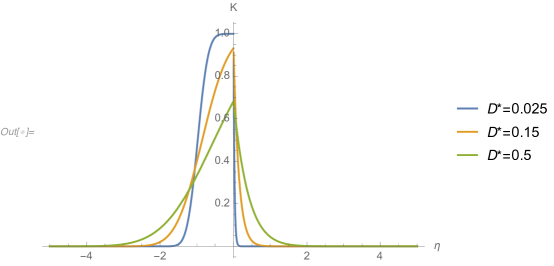
Figure 1: Plot of $\mathcal{K}(\eta,D^{*})$ for several values of $D^{*}$.

These developments lead to the following time-discrete formulation:

$$f^{n+1}(\mathbf{z})=\int_{-\infty}^{\infty}d\tau^{\prime}f^{n}[\hat{\mathbf{z}}(\tau^{\prime};\mathbf{z})]G\left(-\tau^{\prime},\frac{\Delta t}{\epsilon},D^{*}\right)+\Delta t\int_{-\infty}^{\infty}d\tau^{\prime}S(\hat{\mathbf{z}}(\tau^{\prime};\mathbf{z}),t^{n+\theta})\mathcal{L}\left(\tau^{\prime},\frac{\Delta t}{\epsilon},D^{*}\right),$$

where:

$$G\left(\tau,\frac{\Delta t}{\epsilon},D^{*}\right)=\frac{\epsilon}{\Delta t}\mathcal{G}(\eta,D^{*}),$$

with:

$$\mathcal{G}(\eta,D^{*})=\frac{1}{\sqrt{4\pi D^{*}}}e^{-(\eta-1)^{2}/4D^{*}}.$$

Calling:

$$\mathcal{I}\left(f^{n};\mathbf{z},\frac{\Delta t}{\epsilon},D^{*}\right) = \int_{-\infty}^{\infty}d\eta^{\prime}f^{n}[\hat{\mathbf{z}}(\tau^{\prime}=\eta^{\prime}\Delta t/\epsilon;\mathbf{z})]\mathcal{G}(-\eta^{\prime},D^{*}),$$ (38)

$$\mathcal{P}\left(S^{n+\theta};\mathbf{z},\frac{\Delta t}{\epsilon},D^{*}\right) = \int_{-\infty}^{\infty}d\eta^{\prime}S(\hat{\mathbf{z}}(\tau^{\prime}=\eta^{\prime}\Delta t/\epsilon;\mathbf{z}),t^{n+\theta})\mathcal{K}\left(\eta^{\prime},D^{*}\right),$$ (39)

we finally arrive to the discrete temporal update sought:

$$f^{n+1}(\mathbf{z})\approx\mathcal{I}\left(f^{n};\mathbf{z},\frac{\Delta t}{\epsilon},D^{*}\right)+\Delta t\mathcal{P}\left(S^{n+\theta};\mathbf{z},\frac{\Delta t}{\epsilon},D^{*}\right).$$ (40)

This scheme is entirely analogous to the one proposed in Ref. [20] for anisotropic diffusion. A generalization to second-order backward differentiation formulas can be found in the reference.

However, Eq. 40 remains expensive, as the source $S^{n+\theta}$ requires evaluation of the collision operator using the new-time solution, $f^{n+1}$, and is therefore implicitly coupled. To resolve this difficulty, we follow the reference and consider a first-order accurate operator-split (OS) semi-Lagrangian algorithm as follows:

• Implicit Eulerian step:

  $$f^{*}(\mathbf{z})=f^{n}(\mathbf{z})+\Delta t\,\left(\theta S[f^{*}]+(1-\theta)S[f^{n}]\right).$$ (41)

  Choosing $\theta=1$ (backward-Euler or BDF1) is consistent with the order of the overall scheme. This step just requires the integration of the (generally nonlinear) collisional source, perhaps with additional terms for the electric field or radiation forces. We accomplish this here with the algorithm proposed in Ref. [14].

• Lagrangian transport step:

  $$f^{n+1}(\mathbf{z})=\mathcal{I}\left(f^{n};\mathbf{z},\frac{\Delta t}{\epsilon}\right)+\mathcal{P}\left(f^{*}-f^{n};\mathbf{z},\frac{\Delta t}{\epsilon}\right).$$ (42)

  This is a post-processing step (since all fields in the orbit integrals are known) that requires performing an orbit integration (with either Eq. 8 or 11) per phase-space mesh point.

As we shall see in the next section, the algorithm can be made absolutely stable by the judicious choice of $D^{*}$, and is uniformly convergent in $\Delta t/\epsilon$. The numerical implementation details are very similar to those in Ref. [20], and will be reviewed later in this study.

3.3 Stability analysis

We consider the operator-split semi-Lagrangian formulation in the previous section using a backward Euler integration of the source term. We assume the source is a linear functional of the dependent variable, $f$. We assume orbits are straight in this analysis. Fourier-analyzing Eq. 42 gives:

$$f_{\mathbf{k}}^{n+1}=e^{-L(k_{\parallel}\Delta t/\epsilon,D^{*})}f_{\mathbf{k}}^{n}-\Delta t\,S_{\mathbf{k}}f_{\mathbf{k}}^{*}\frac{1-e^{-L(k_{\parallel}\Delta t/\epsilon,D^{*})}}{L(k_{\parallel}\Delta t/\epsilon,D^{*})},$$

with $f_{\mathbf{k}}^{n+1}$ the Fourier amplitude of the new-time PDF for wavenumber $\mathbf{k}$, $f_{\mathbf{k}}^{*}$ the same for the solution of the first step in the OS algorithm, $k_{\parallel}=\mathbf{k}\cdot\mathbf{b}$ the wavenumber along the orbit, $S_{\mathbf{k}}=S_{r}+iS_{i}$ the amplitude of the Fourier transform of the (linearized) source, and

$$L(\xi,D^{*})=i\xi+D^{*}\xi^{2}.$$ (43)

The convenience of the choice of the diffusion coefficient $D$ in Eq. 36 is now apparent, as it leads to a very simple functional form of the amplification factor $\frac{f_{\mathbf{k}}^{n+1}}{f_{\mathbf{k}}^{n}}$ in terms of $\xi=k_{\parallel}\Delta t/\epsilon$. In the Fourier transform of the source, the real component corresponds to the collisional term (which is self-adjoint), and the imaginary one to possible advective transport terms in momentum space (e.g., E-field, radiation force). The Fourier transform of the backward-Euler integration step (Eq. 41) gives:

$$f_{\mathbf{k}}^{*}=\frac{f_{\mathbf{k}}^{n}}{1+\Delta t\,S_{\mathbf{k}}}.$$

There results the complex amplification factor:

$$\lambda(\xi,D^{*},S_{\mathbf{k}})=\frac{f_{\mathbf{k}}^{n+1}}{f_{\mathbf{k}}^{n}}=e^{-L(\xi,D^{*})}-\frac{\Delta t\,S_{\mathbf{k}}}{1+\Delta t\,S_{\mathbf{k}}}\frac{1-e^{-L(\xi,D^{*})}}{L(\xi,D^{*})}.$$

Stability requires:

$$M_{\lambda}(\xi,D^{*},S_{\mathbf{k}})=|\lambda(\xi,D^{*},S_{\mathbf{k}})|<1.$$

To find the stability boundary in $D^{*}$, we maximize $M_{\lambda}(\xi,D^{*},S_{\mathbf{k}})$ for each value of $D^{*}$, with $\Delta tS_{r}<1$ (i.e., assuming dynamical collisional timescales are resolved, but still allowing for implicit timesteps much larger than numerical stability constraints) in the domain $\xi\in[0,5]$, $\Delta tS_{i}\in[0,1]$. This maximum is found to be monotonically decreasing with $D^{*}$. The result for $D^{*}\in[0,0.5]$ is depicted in Fig. 2 for various values of $\Delta tS_{r}=\Delta tk_{v}^{2}$ (with $k_{v}^{2}$ a measure of the magnitude of the collisional source Fourier amplitude), and demonstrates stability for $D^{*}\gtrsim 0.125$. If the source is purely collisional, i.e., $S_{i}=0$, the same analysis indicates stability for $D^{*}\gtrsim 0.025$ (not shown). As will be shown, the computational cost of the orbit integrals scales as $\sqrt{D^{*}}$, and therefore the latter may be in principle more efficient. However, as we shall see, this efficiency gain is offset by the cost of reduced outer timesteps, required to preserve accuracy because of the implied splitting between the electric field acceleration term and collisions. As a result, treating acceleration terms on the momentum mesh is more efficient in practice.

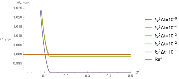
Figure 2: Plot of maximum amplification factor vs. $D^{*}$ for various collisional strengths $S_{r}=k_{v}^{2}$.

3.4 Asymptotic-preserving character of the semi-Lagrangian algorithm: limit solution

We begin with the propagator step of the operator-split semi-Lagrangian algorithm (Eq. 42):

$$f^{n+1}(\mathbf{z})=\mathcal{I}\left(f^{n};\mathbf{z},\frac{\Delta t}{\epsilon}\right)+\mathcal{P}\left(f^{*}-f^{n};\mathbf{z},\frac{\Delta t}{\epsilon}\right),$$ (44)

where $f^{*}$ is found from updating the source only (Eq. 41), and the propagators $\mathcal{I}$ and $\mathcal{P}$ are defined in Eqs. 38 and 39, respectively, and reproduced here considering an arbitrary $\eta=\epsilon\tau/\Delta t$ as the starting point of the orbit integrals (instead of $\eta=0$):

$$\mathcal{I}\left(f^{n};\mathbf{z}(\eta),\frac{\Delta t}{\epsilon},D^{*}\right) = \int_{-\infty}^{\infty}d\eta^{\prime}f^{n}[\hat{\mathbf{z}}(\tau^{\prime}=\eta^{\prime}\Delta t/\epsilon;\mathbf{z})]\mathcal{G}(\eta-\eta^{\prime},D^{*}),$$ (45)

$$\mathcal{P}\left(S^{n+\theta};\mathbf{z}(\eta),\frac{\Delta t}{\epsilon},D^{*}\right) = \int_{-\infty}^{\infty}d\eta^{\prime}S(\hat{\mathbf{z}}(\tau^{\prime}=\eta^{\prime}\Delta t/\epsilon;\mathbf{z}),t^{n+\theta})\mathcal{K}\left(\eta^{\prime}-\eta,D^{*}\right).$$ (46)

The kernels $\mathcal{G}$ and $\mathcal{K}$ are normalized:

$$\int_{-\infty}^{\infty}d\eta\mathcal{G}(\eta-\eta^{\prime},D^{*}) = \int_{-\infty}^{\infty}d\eta\mathcal{K}(\eta-\eta^{\prime},D^{*})=1.$$

Therefore, integrating Eqs. 45 and 46 with respect to $\eta$, and using the definition of the bounce-averaging operator in Eq. 29, gives:

$$\int_{-\infty}^{\infty}d\eta\mathcal{I}\left(f^{n};\mathbf{z}(\eta),\frac{\Delta t}{\epsilon},D^{*}\right) = \int_{-\infty}^{\infty}d\eta^{\prime}f^{n}[\hat{\mathbf{z}}(\tau^{\prime}=\eta^{\prime}\Delta t/\epsilon;\mathbf{z})]=\frac{\epsilon}{\Delta t}\left\langle f^{n}\right\rangle\int_{-\infty}^{\infty}ds^{\prime}/B,$$

$$\int_{-\infty}^{\infty}d\eta\mathcal{P}(f^{*}-f^{n};\mathbf{z}(\eta),\Delta t) = \int_{-\infty}^{\infty}d\eta^{\prime}(f^{*}[\hat{\mathbf{z}}(\tau^{\prime}=\eta^{\prime}\Delta t/\epsilon;\mathbf{z})]-f^{n}[\hat{\mathbf{z}}(\tau^{\prime}=\eta^{\prime}\Delta t/\epsilon;\mathbf{z})])=\frac{\epsilon}{\Delta t}\left\langle f^{*}-f^{n}\right\rangle\int_{-\infty}^{\infty}ds^{\prime}/B.$$

Introducing these results in Eq. 44 and using Eq. 41, yields the following first-order-accurate discrete integral of the asymptotic limit equation:

$$\left\langle f^{n+1}\right\rangle=\left\langle f^{*}\right\rangle=\left\langle f^{n}\right\rangle+\Delta t\left\langle S[f^{*}]\right\rangle.$$

We have thus proved that the limit solution of the semi-Lagrangian formulation for $\epsilon\rightarrow 0$ is in fact the bounce-averaged solution, and therefore the algorithm is asymptotic-preserving (AP).

3.5 Asymptotic properties of semi-Lagrangian scheme: error analysis and uniform convergence

We demonstrate next that the semi-Lagrangian algorithm is not only AP, but uniformly convergent in $\Delta t/\epsilon$. We begin by considering the rDKE equation in thermal units along relativistic orbits ($\mathcal{E}=\gamma-\Phi,\mu$), including the regularizing diffusion term:

$$\partial_{t}f+\frac{1}{\epsilon}\partial_{\tau}f-\frac{D^{*}\Delta t}{\epsilon^{2}}\partial_{\tau}^{2}f=C(f).$$ (47)

As before (Sec. 2.2), we begin the asymptotic analysis by considering a Hilbert expansion for $\epsilon\ll 1$:

$$f=f_{0}+\epsilon^{\alpha}f_{1}+\ldots$$ (48)

Here, $\left\langle f\right\rangle=\left\langle f_{0}\right\rangle$ (constant along orbits), and $f_{i>0}\sim\mathcal{O}(1)$, but $\left\langle f_{i>0}\right\rangle=0$. Introducing this expansion into Eq. 47, we find:

$$\partial_{t}(f_{0}+\epsilon^{\alpha}f_{1})+\epsilon^{\alpha-1}\partial_{\tau}f_{1}-\epsilon^{\alpha-2}D^{*}\Delta t\partial_{\tau}^{2}f_{1}+HOT(\epsilon)=C(f),$$

where the source behaves regularly with $\epsilon$ (i.e., has no $1/\epsilon$ dependence), and $\alpha\geq 1$ for regularity of the advective term (otherwise it would imply $f_{1}=0$). Taking the average of this equation, we get the limit equation:

$$\partial_{t}\left\langle f_{0}\right\rangle=\left\langle C(f)\right\rangle,$$

and therefore:

$$\epsilon^{\alpha}\partial_{t}f_{1}+\epsilon^{\alpha-1}\partial_{\tau}f_{1}-\epsilon^{\alpha-2}D^{*}\Delta t\partial_{\tau}^{2}f_{1}+HOT(\epsilon)=C(f_{0})-\left\langle C\right\rangle=\mathcal{O}(1).$$

The last equality is justified because $C(f_{0})=C(\left\langle f\right\rangle)\neq\left\langle C(f)\right\rangle$ in general. Since $\alpha\geq 1$, matching $\epsilon$ powers, we get:

$$\epsilon^{\alpha-2}D^{*}\Delta t\partial_{\tau}^{2}f_{1}=\mathcal{O}(1).$$

Since $f_{1}\sim\mathcal{O}(1)$ by ansatz, and taking $\partial_{\tau}f_{1}=ik_{\parallel}f_{1}$, it follows that:

$$\epsilon^{\alpha-2}D^{*}\Delta tk_{\parallel}^{2}\sim 1.$$

This suggests $\alpha=2$ (which will be verified numerically) and consequently that the diffusion Fourier-mode cut-off (which controls the asymptotic transition) happens at $k_{\parallel,\mathrm{cutoff}}\sim 1/(D^{*}\Delta t)^{1/2}$. It also follows that:

$$\xi_{\mathrm{cutoff}}=k_{\parallel}\Delta t/\epsilon\sim\epsilon^{-1}(\Delta t/D^{*})^{1/2}\,\,;\,\,f=f_{0}+\mathcal{O}(\epsilon^{2}).$$

With these results, we are equipped to study the temporal discretization error of the semi-Lagrangian algorithm. Asymptotic error of convergence is expected to be first-order, both from its OS character and the BDF1 treatment of the Eulerian step. The sources of temporal discretization error are the constant-source approximation and the operator splitting. We analyze these next. The analysis exactly follows that in Ref. [20] (Appendices B and C in the reference).

We begin with the splitting error. Ref. [20] gives the following expression for the global truncation error (GTE, defined as the accumulated temporal error for the total timespan of a given simulation) due to splitting:

$$\mathcal{E}_{split}^{GTE}\sim k_{v}^{2}\left|f_{\mathbf{k}}\right|\left|1-e^{-L(\xi,D^{*})}\right|\sim k_{v}^{2}\left|f_{\mathbf{k}}\right|\min[\xi,1].$$

Here, $L(\xi,D^{*})$ is defined in Eq. 43, and, as before, $k_{v}^{2}$ is a measure of the Fourier-transform amplitude of the (linearized and self-adjoint) collision operator. From this expression, it is apparent that the splitting error strictly vanishes for the limit solution ($k_{\parallel}=0$), since $\xi=0$ in that case. For finite $k_{\parallel}$, using the results in the previous section (and in particular that $f_{\mathbf{k}}\sim\epsilon^{2}$ for finite $k_{\parallel}$ and small enough $\epsilon$), we readily conclude that:

$$\mathcal{E}_{split}^{GTE}(k_{\parallel}\neq 0)\sim\begin{cases}\xi\sim\Delta t&\xi\ll 1\\ \epsilon(\Delta t/D^{*})^{1/2}&\xi\sim\xi_{\mathrm{cutoff}}\\ \epsilon^{2}&\xi\gg 1\end{cases}.$$

This result proves uniform convergence with respect to $\xi\sim\Delta t/\epsilon$: it is first-order accurate (as expected) and independent of $D^{*}$ for resolved modes ($\xi\ll 1$), and scales as $\epsilon^{2}$ in the asymptotic regime for unresolved ones ($\xi\gg 1$). At the transition, we find the error scales as the geometric mean of the two, $\epsilon\sqrt{\Delta t/D^{*}}$, showing a weak dependence on $D^{*}$. These conclusions will be verified numerically in Sec. 5.

Since the splitting error vanishes for the limit solution ($k_{\parallel}=0$), its error is determined by the constant-source approximation in Eq. 35. Following Ref. [20], the global truncation error for the OS+BDF1 algorithm can be written as:

$$\mathcal{E}_{src}^{GTE}\sim k_{v}^{2}\Delta t\left|\partial_{t}f_{\mathbf{k}}\frac{\left[1+\hat{L}(\xi)\right]e^{-\hat{L}(\xi)}-1}{[\hat{L}(\xi)]^{2}}\right|.$$

Here,

$$\partial_{t}f_{\mathbf{k}}\sim\frac{f_{\mathbf{k}}}{\tau_{k}},$$

with $\tau_{k}$ the time constant for the Fourier mode $\mathbf{k}=(k_{\parallel},k_{v})$, which is found from the original equation, Eq. 47, as:

$$\frac{\Delta t}{\tau_{k}}\sim|\hat{L}(\xi)+k_{v}^{2}\Delta t|.$$

There results:

$$\mathcal{E}_{src}^{GTE}\sim k_{v}^{2}\left|f_{\mathbf{k}}\right||\hat{L}(\xi)+k_{v}^{2}\Delta t|\left|\frac{\left[1+\hat{L}(\xi)\right]e^{-\hat{L}(\xi)}-1}{[\hat{L}(\xi)]^{2}}\right|\sim\begin{cases}k_{v}^{4}\Delta t&\xi\ll 1\\ \frac{k_{v}^{2}\left|f_{\mathbf{k}}\right|}{D^{*}\xi^{2}}\sim\epsilon^{4}&\xi\gg 1\end{cases},$$

where we have used that $\left|f_{\mathbf{k}}\right|\sim\epsilon^{2}$ for $k_{\parallel}\neq 0$ and $\xi\gg 1$. The constant-source error is first-order for resolved modes (and in particular for the limit solution with $k_{\parallel}=0$), and scales as $\epsilon^{4}$ otherwise (i.e., it is negligible compared to the OS error).

4 Numerical implementation details

The numerical integration of the collision operator on the Eulerian mesh is performed as described in Ref. [14]. Even though our collisional implementation is in principle fully nonlinear, in certain tests we have considered a linearized implementation of the collision operator (in which the background electron population does not evolve) for some of the comparisons below for consistency with the original references.

The numerical implementation of the Lagrangian integrals along orbits largely follows the details outlined in Ref. [20]. As in the reference, a numerical implementation of the propagators (Eqs. 38, 39) requires three elements: a suitable orbit integrator, a suitable interpolation procedure of the function $f(\mathbf{z})$ from the computational mesh to the orbit position, and a sufficiently accurate numerical quadrature of integrals along orbits. For interpolation, we consider both second-order multidimensional global and local splines in a structured, non-uniform logical mesh. The former is potentially more accurate but more expensive, while the latter is significantly cheaper but potentially less accurate. Here, we consider both to assess the practical accuracy of the local spline interpolation approach for non-uniform meshes (described in detail in B). Unless otherwise noted, results reported here have been obtained with the local interpolation approach. We limit our interpolation order to second order to ensure sufficient accuracy while minimizing the chances of producing negative values, which is of concern since the PDF tails can be quite rarefied and can be significantly distorted by negative values. In the instances where negative interpolated values for PDFs are found along orbits, we reset them to zero in the global spline, and revert to first-order interpolation in the local spline.

Orbits and quadratures along orbits are computed simultaneously using the high-order ODE integration package ODEPACK [23], which features highly efficient, adaptive, high-order (up to 12th order) numerical ODE integration routines. By treating the orbits and the propagator integral on the same footing, ODEPACK is able to adapt to structure in both the orbits and the integrands. The ODE set in Eqs. 8 and 11 is not stiff, and a simple Picard-implicit time-stepping integrator is sufficient. The simulations presented in this study have been obtained with very tight relative and absolute convergence tolerances for the ODE solver ($10^{-12}$), to minimize the impact of orbit integration errors on the error convergence studies. The code is fully parallelized with MPI, and orbits are threaded using OpenMP.

The numerical integration in Eqs. 38 and 39 is performed along two semi-infinite orbit domains, $\eta^{\prime}\in[0,\infty)$ and $\eta^{\prime}\in(-\infty,0]$. Orbits are numerically truncated according to error estimates based on the left-over integrals of the kernels, which are estimated here (using similar techniques to those documented in Ref. [20]) for a given tolerance $\varepsilon$ as:

$$\int_{\eta_{cut}}^{\infty}d\eta^{\prime}\mathcal{G}(-\eta^{\prime},D^{*})<\varepsilon \Rightarrow \eta_{cut}=2\sqrt{D^{*}}\xi_{cut}-1\,;\,\xi_{cut}\gtrsim\sqrt{|\ln(2\varepsilon\sqrt{\pi}\xi_{cut})|},$$

$$\int_{-\infty}^{-\eta_{cut}}d\eta^{\prime}\mathcal{G}(-\eta^{\prime},D^{*})<\varepsilon \Rightarrow \eta_{cut}=2\sqrt{D^{*}}\xi_{cut}+1\,;\,\xi_{cut}\gtrsim\sqrt{|\ln(2\varepsilon\sqrt{\pi}\xi_{cut})|},$$

$$\int_{\eta_{cut}}^{\infty}d\eta^{\prime}\mathcal{K}(\eta^{\prime},D^{*})<\varepsilon \Rightarrow \eta_{cut}=2\sqrt{D^{*}}\xi_{cut}\,;\,\xi_{cut}\gtrsim-\frac{1}{2\sqrt{D^{*}}}+\sqrt{\left|\ln\left(\varepsilon\sqrt{\pi}\xi_{cut}^{3/2}\left(\xi_{cut}+\frac{1}{2\sqrt{D^{*}}}\right)^{1/2}\right)\right|},$$

$$\int_{-\infty}^{-\eta_{cut}}d\eta^{\prime}\mathcal{K}(\eta^{\prime},D^{*})<\varepsilon \Rightarrow \eta_{cut}=2\sqrt{D^{*}}\xi_{cut}\,;\,\xi_{cut}\gtrsim\frac{1}{2\sqrt{D^{*}}}+\sqrt{\left|\ln\left(\varepsilon\sqrt{\pi}\xi_{cut}^{3/2}\left(\xi_{cut}-\frac{1}{2\sqrt{D^{*}}}\right)^{1/2}\right)\right|}.$$

In these expressions, $\xi_{cut}$ can be found very quickly for a prescribed tolerance $\varepsilon$ once at the beginning of the simulation with a few Picard iterations. The asymmetry in the integral bounds with respect to the sign of $\eta$ originates in the advective character of the $\mathcal{G}$ and $\mathcal{K}$ kernels. It is worth noting that the integral bound cutoff in the original integration variable $\tau=\Delta t\eta/\epsilon$ is roughly proportional to $\Delta t\sqrt{D^{*}}/\epsilon$, indicating that the cost of the orbit integrals will grow accordingly.

We finalize this section commenting on the conservation properties of the semi-Lagrangian approach. The nonlinear collisional source is fully conservative in mass, momentum, and energy [14]. The Lagrangian step is also conservative in the continuum, but in principle not in the discrete. We enforce mass conservation errors (typically of 1 part in $10^{7}$ after the orbit integration) by renormalizing our PDF after the Lagrangian update to the integrated mass before the update. This strategy corrects for long-term error accumulation. We do not correct for errors in momentum or energy conservation. We will demonstrate numerically in the next section that these remain small, $\sim\mathcal{O}(10^{-9})$, in typical simulations.

5 Numerical results

We consider several tests in increasing order of complexity to demonstrate the asymptotic properties and correctness of the semi-Lagrangian algorithm. We begin with a 0D-2P Dreicer generation test problem, which allows us to compare the semi-Lagrangian implementation to a purely Eulerian one. We demonstrate that both agree very well with each other, and with documented results elsewhere in the literature. Next, following Ref. [6], we consider the runaway-electron Dreicer generation rate in a 2D axisymmetric circular tokamak geometry. We use this nontrivial geometry to demonstrate the conservation properties of the semi-Lagrangian scheme, and verify our implementation against the results in the reference, demonstrating excellent agreement. We also use this test to demonstrate the advertised asymptotic properties of the scheme, namely, uniform convergence in $\Delta t/\epsilon$, and the asymptotic convergence to the limit (bounce-averaged [4]) solution.

5.1 0D-2P Dreicer generation problem

We consider first a 0D-2P Dreicer runaway generation problem with no magnetic field. The purpose of this test is to verify the simplest semi-Lagrangian scheme (where only the electric field is treated in a Lagrangian manner) against the fully Eulerian implementation in Ref. [14]. The orbit equations for the semi-Lagrangian algorithm in this case simply become:

$$\frac{dp_{\parallel}}{d\tau}=-E_{\parallel}.$$

Unless otherwise specified, we consider a Dreicer-normalized electric field $E_{\parallel}=0.06$, and a plasma temperature of 100 eV ($\Theta_{0}=(v_{th}/c)^{2}=1.95\times 10^{-4}$). The normalized momentum domain is $p_{\parallel}\in(-0.3,1.2)$, $p_{\perp}\in(0,0.5)$, with a 512$\times$128 hybrid uniform-geometric mesh, with a 256$\times$32 uniform mesh resolving the thermal bulk in $p_{\parallel}\in(-5v_{th}/c,5v_{th}/c)$ and $p_{\perp}\in(0,5v_{th}/c)$ (with $5v_{th}/c\approx 0.07$), and expanding geometrically from there to the outer domain limits with the remaining mesh points. The domain limits in $p_{\parallel}$ were chosen such that a sufficient runaway tail can be measured by our Dreicer production diagnostic. The timestep used is $\Delta t=5\times 10^{-7}$ in relativistic units ($\approx 0.18$ thermal collision times) for the Eulerian simulation (which we term “Eulerian-$E$” to highlight the fact that the electric field is treated on the mesh), and $\Delta t=1\times 10^{-7}$ and $D^{*}=0.05$ for the semi-Lagrangian ones (which we term “Lagrangian-$E$” to highlight the fact that the electric field is integrated along orbits). As we show below, larger timesteps in the Lagrangian-$E$ treatment result in significant deviation of the Dreicer generation rate vs. the Eulerian result owing to the splitting introduced between collisions and acceleration terms. We run the simulation to $t=2.5\times 10^{-3}$, or 900 thermal collision times. A sample hybrid uniform-geometric 128x64 mesh on a similar domain is provided in Fig. 3, along with the Eulerian solution at 900 $\tau_{c}^{th}$.

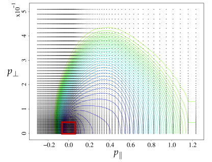
Figure 3: Sample hybrid uniform-geometric mesh employed in the 0D-2P Dreicer generation problem, along with Eulerian-$E$ solution at $t=900\tau_{c}^{th}$. This particular mesh has 128$\times$64 points, with a uniform mesh (red box) of 32$\times$16 points resolving the bulk Maxwellian in $p_{\parallel}\in(-3.5v_{th}/c,3.5v_{th}/c)$ and $p_{\perp}\in(0,3.5v_{th}/c)$ (with $3.5v_{th}/c\approx 0.05$), and expanding geometrically from there to the domain limits.

The Dreicer production rate (in relativistic collision time units) $\sigma_{rel}$ is measured as:

$$\sigma_{rel}=\frac{\partial_{t}n_{RE}}{n_{0}-n_{RE}},$$

where $n_{0}$ is the initial electron density, and $n_{RE}$ is the runaway electron population, which is measured from the solution for electron velocities exceeding $p_{cutoff}\approx$ 25 $v_{th}/c\approx 0.35$ in the positive $p_{\parallel}$ domain, i.e.:

$$n_{RE}=\int_{p_{\parallel,cutoff}}^{\infty}dp_{\parallel}\int_{p_{\perp,cutoff}}^{\infty}dp_{\perp}p_{\perp}f,$$

with $p_{\parallel,cutoff}^{2}+p_{\perp,cutoff}^{2}\geq p_{cutoff}^{2}$ and $p_{\parallel,cutoff}>0$.

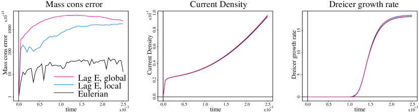
Figure 4: Comparison of the Eulerian and semi-Lagrangian time histories of mass conservation error, Dreicer current density generation, and Dreicer growth rate for the 0D-2P Dreicer generation problem, demonstrating excellent agreement.

Figure 4 depicts the comparison of time traces of mass conservation error, kinetic energy, current density carried by runaway electrons, and Dreicer growth rate from both Eulerian and semi-Lagrangian implementations (the latter using both global and local interpolation of the propagator integrands), demonstrating excellent agreement in all cases. For these cold plasma conditions, we can compare the Dreicer generation rate against the results in Ref. [24] (which were obtained with a non-relativistic collisional treatment) to find excellent agreement ($\sigma_{rel}=18.3$ in the figure vs. $\sigma_{rel}=\sigma(c/v_{th})^{3}=18.5$, with $\sigma=5\times 10^{-5}$, in the reference). This suggests that the results in Fig. 4 are converged. The semi-Lagrangian 0D run with local interpolation is a factor of two faster (in wall-clock time) than the global-spline run. In these results, the Lagrangian-$E$ treatment uses a timestep $5\times$ smaller than the Eulerian-$E$ run for accuracy.

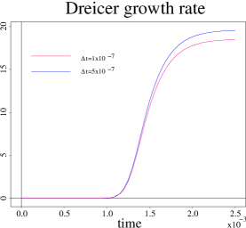
Figure 5: Impact of timestep size in the accuracy of the computation of the 0D-2P Dreicer growth rate with the Lagrangian-$E$ treatment. The larger timestep ($\Delta t=5\times 10^{-7}$, which gives an accurate solution with the Eulerian-$E$ treatment) results in significant overestimation of the Dreicer growth rate by the Lagrangian-$E$ treatment. This outcome is insensitive to the choice of interpolation in the semi-Lagrangian algorithm.

Figure 5 illustrates the accuracy impact in the Dreicer growth rate when a larger time step is used in the Lagrangian-$E$ simulation. For the same timestep as in the Eulerian-$E$ treatment ($\Delta t=5\times 10^{-7}$), the semi-Lagrangian simulation introduces significant error in the Dreicer growth rate, indicating that the Eulerian-$E$ treatment is preferable from an accuracy standpoint for a given timestep. Results in the next section confirm that this conclusion applies to 2D-2P simulations as well.

5.2 2D-2P Dreicer generation in axisymmetric tokamak

In principle, our proposed algorithm can deal with general three-dimensional magnetic field configurations. In this study, we consider 2D axisymmetric toroidal topologies, of recent interest [6]. In such topologies, the magnetic field can be described by an axisymmetric poloidal flux function $\Psi$ (i.e., independent of the toroidal angle $\phi$), and a toroidal magnetic field $B_{\phi}$ as:

$$\mathbf{B}=\nabla\phi\times\nabla\Psi+RB_{\phi}\nabla\phi.$$

Clearly, $\mathbf{B}$ is tangential to flux surfaces, and the orbit dynamics can be described by a poloidal angle $\theta$ along a given flux surface, $\Psi$. Therefore, the spatial dependence of the PDF can be described uniquely by the coordinates ($\Psi,\theta$), and we have:

$$f=f(\Psi,\theta,p_{\parallel},p_{\perp}).$$

Figure 6: Sketch of axisymmetric cylindrical tokamak geometry.

We consider the same geometry as in Ref. [6], i.e., a circular tokamak geometry of normalized radius $a=1$ (see Fig. 6), with the q-profile given by:

$$q(r)=\frac{rB_{\phi}}{RB_{\theta}}=2.1+2r^{2}.$$

Here, $r$ is the toroidal minor radius, which in this configuration is a flux function and therefore can replace $\Psi$ as a coordinate. The corresponding poloidal and toroidal magnetic field components ($B_{\theta},B_{\phi})$ are given by:

$$B_{\phi} = \frac{R_{0}B_{0}}{R}=\frac{B_{0}}{1+\frac{r}{R_{0}}\cos(\theta)},$$

$$B_{\theta} = \frac{rB_{\phi}}{R_{0}q(r)},$$

with $R_{0}=3a$ the toroidal major radius [6] and $B_{0}$ a reference magnetic field (which can be set to unity without loss of generality, as it does not enter the final orbit equations). The corresponding magnetic field magnitude is:

$$B=\sqrt{B_{\theta}^{2}+B_{\phi}^{2}}=B_{\phi}\sqrt{1+\left(\frac{r}{qR_{0}}\right)^{2}}.$$

In circular geometry, the orbit equations in relativistic units (Eq. 8 or Eq. 11, depending on the representation) can be simplified as:

$$\frac{d\theta}{d\tau} = \frac{d\mathbf{x}}{d\tau}\cdot\frac{\partial\theta}{\partial\mathbf{x}}=\frac{d\mathbf{x}}{d\tau}\cdot\frac{\boldsymbol{\theta}}{r}=\frac{p_{\parallel}}{\gamma}\frac{B_{\theta}}{rB},$$ (49)

$$\frac{dp_{\parallel}}{d\tau} = \left[-E_{\parallel}\right]-\frac{p_{\perp}^{2}}{2\gamma}\frac{\mathbf{b}\cdot\nabla B}{B}=\left[-E_{\parallel}\right]-\frac{p_{\perp}^{2}}{2\gamma}\frac{B_{\theta}\partial_{\theta}B}{rB^{2}},$$ (50)

$$\frac{dp_{\perp}}{d\tau} = \frac{p_{\perp}p_{\parallel}}{2\gamma}\frac{\mathbf{b}\cdot\nabla B}{B}=\frac{p_{\perp}p_{\parallel}}{2\gamma}\frac{B_{\theta}\partial_{\theta}B}{rB^{2}},$$ (51)

where:

$$\frac{B_{\theta}}{B}=\frac{r}{\sqrt{(R_{0}q)^{2}+r^{2}}}\,\,;\,\,\frac{\partial_{\theta}B}{rB}=\frac{\sin(\theta)}{R_{0}+r\cos(\theta)}.$$

The parallel (toroidal) electric field $E_{\parallel}$ is defined from a gradient, and therefore in toroidal geometry satisfies:

$$E_{\parallel}=\frac{E_{0}R_{0}}{R}=\frac{E_{0}}{1+\frac{r}{R_{0}}\cos(\theta)},$$

with $E_{0}$ a reference electric field in relativistic (Connor-Hastie) units.

5.2.1 Conservation tests of the semi-Lagrangian algorithm with nonlinear collisions in the absence of external drivers

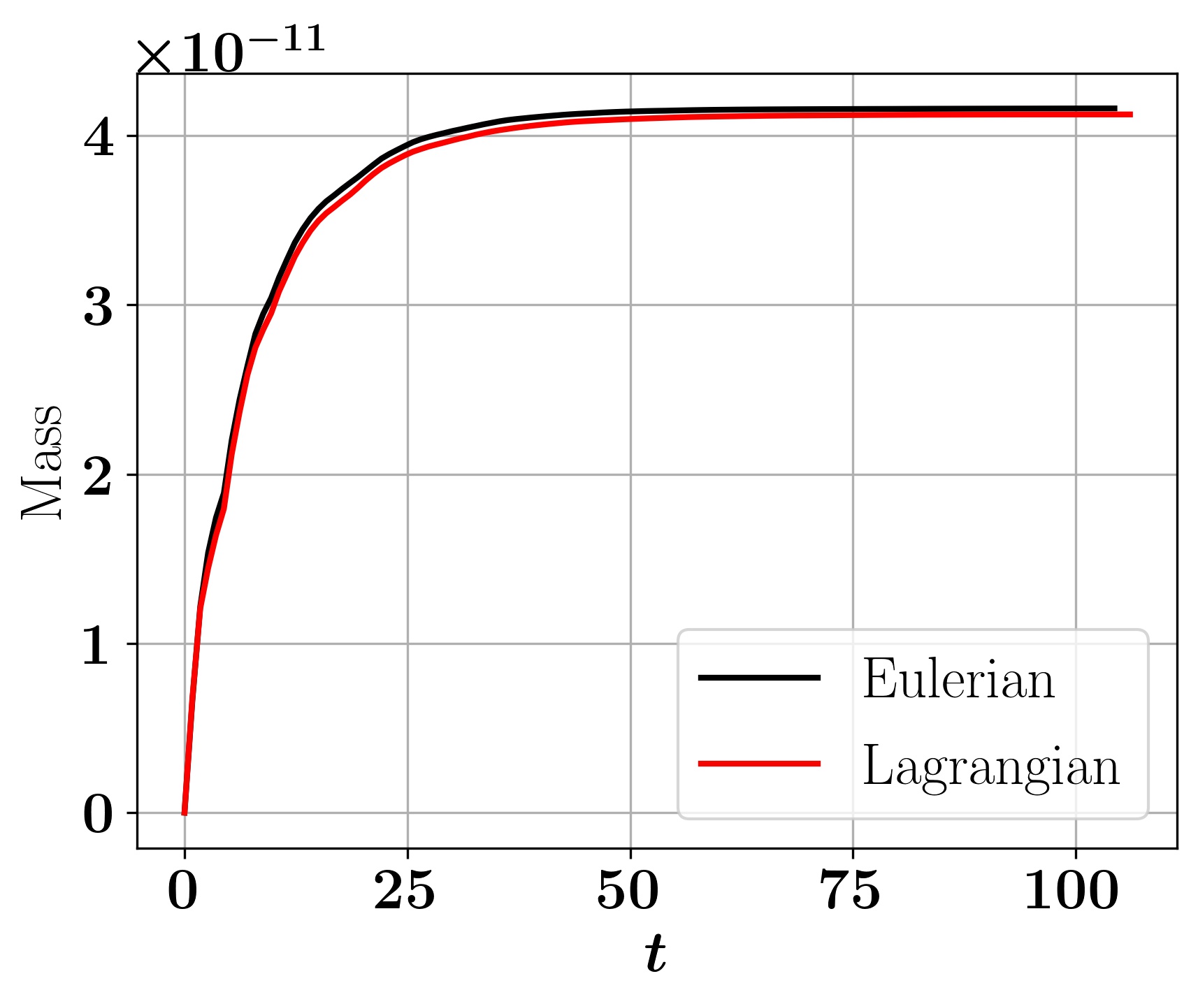
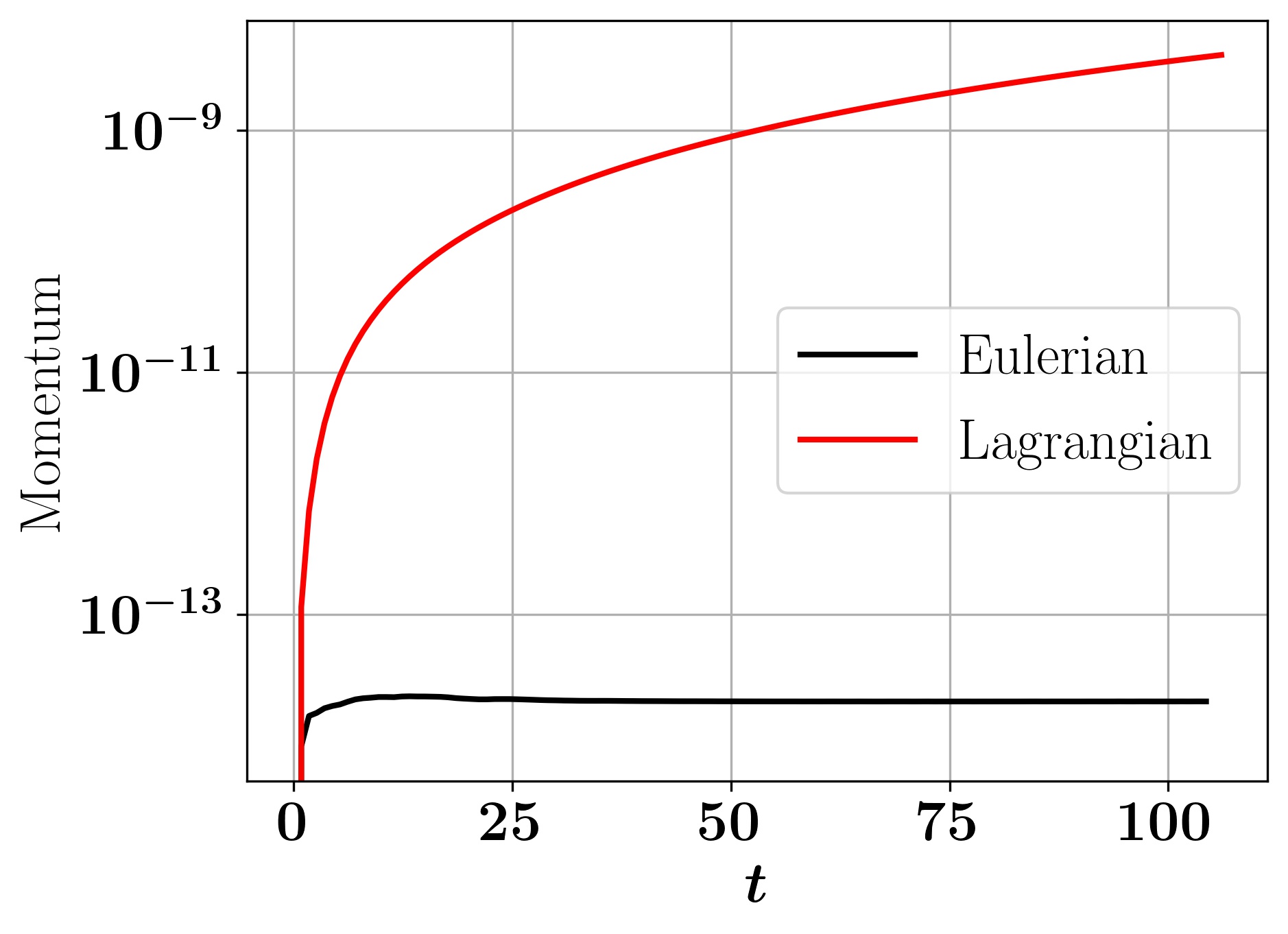
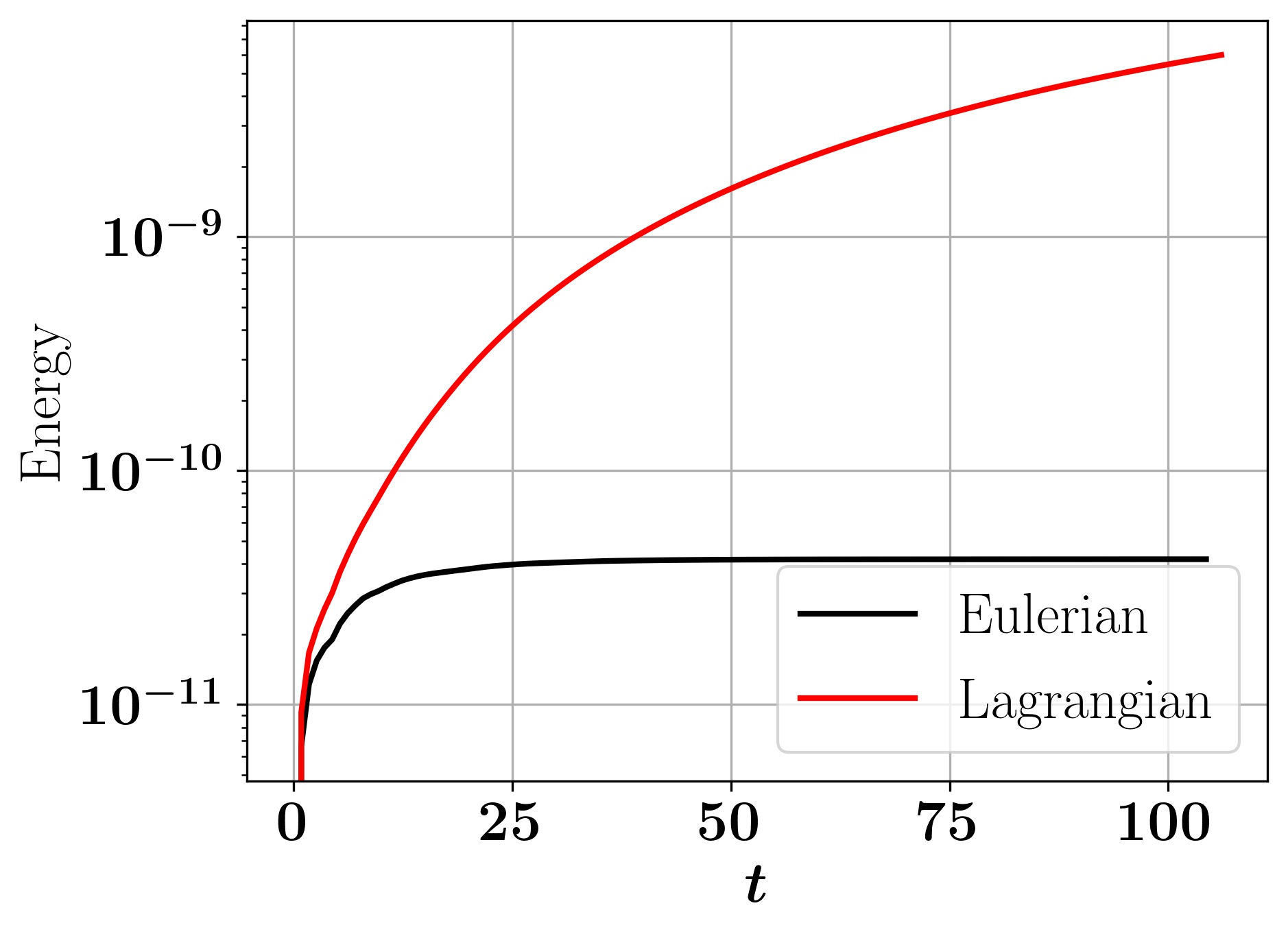
Figure 7: Off-axis ($r/a=0.4$) thermal equilibrium test with no external driver, demonstrating excellent conservation properties of the semi-Lagrangian algorithm (red line) for mass, momentum, and energy. Conservation properties for the Eulerian discretization on-axis ($r=0$, for which the angular coordinate is ignorable, and therefore features no spatial dependence) are provided as a reference (black line).

We begin by testing the conservation properties of the semi-Lagrangian algorithm without external drivers such as an electric field, but including fully nonlinear and conservative electron-electron collisions. We recall that the collisional treatment is fully conservative when solved nonlinearly, as has been documented elsewhere [14]. The test therefore highlights the conservation errors introduced by the transport (collisionless) component. We consider an initial condition in thermal equilibrium for a temperature of 100 eV and $E_{\parallel}=0$ (i.e., no external driver is present). Simulations are performed on a $8\times 128\times 64$ grid with domain size in $p_{\parallel}\in(-0.3,0.3)$ and $p_{\perp}\in(0,0.3)$. Eulerian simulations are performed on-axis ($r=0$), for which the angular direction is ignorable, and are provided here as a reference. Lagrangian simulations were performed off-axis ($r/a=0.4$), using the local interpolation scheme for 100 thermal collisional steps. Results are reported in Fig. 7, and demonstrate the ability of the scheme to conserve invariants in less than one part in $10^{8}$, thus maintaining thermal equilibrium to high precision.

5.2.2 Verification tests

We consider the plasma radii

$$\frac{{r}}{a}=0,0.2,0.4,0.6,0.8,$$

and plasma temperatures of 100eV, 1 keV, and 10 keV. For consistency with Ref. [6], we consider the linearized form of the relativistic collision operator, in which the background electron population does not evolve. To reproduce the results in the reference, the Coulomb logarithm in the collision operator is computed for the given density and temperature values according to well-known formulas [25]. We measure the Dreicer electron production growth rate for an effective ion charge $Z_{\mathrm{{eff}}}=1$ and an electric field $E_{0}=0.06\,E_{D}/E_{CH}=0.06(c/v_{th})^{2}$. Considering a temperature-dependent Coulomb logarithm, $R_{0}=6$ m in physical units, and a density of $n=2\times 10^{14}$ cm^-3, we obtain $\epsilon_{rel}=1.45\times 10^{-6},\,1.73\times 10^{-6},\,2\times 10^{-6}$ (corresponding to $\epsilon=38,\,0.45,\,0.0052$) for 100 eV, 1 keV and 10 keV, respectively. As before, the simulations span a total time of 900-1000 $\tau_{c}^{th}$.

We consider both a Lagrangian-$E$ treatment (Eq. 9) and an Eulerian-$E$ treatment (Eq. 10). From the results of the stability analysis, we choose $D^{*}=0.2$ for all Eulerian-$E$ cases and $D^{*}=0.05$ for all Lagrangian-$E$ cases. Timesteps with the Eulerian-$E$ treatment for the colder plasmas (100 eV and 1 keV) are $\Delta t\approx 0.2$ $\tau_{c}^{th}$ [or, in relativistic (code) units, $\Delta t=0.2(v_{th}/c)^{3}$], while for the hot case (10 keV) we use $\Delta t\approx 0.07$ $\tau_{c}^{th}$. As observed before, the Lagrangian-$E$ treatment requires timesteps a factor of 2 or so smaller than those with an Eulerian-$E$ treatment for good agreement, owing to the additional splitting error introduced when dealing with the electric-field acceleration in the orbit integrals. The nonlinear tolerance is set to $10^{-8}$ and background potentials are solved at the beginning of the simulation with a linear relative tolerance of $10^{-10}.$

We use a geometrically stretched momentum grid of $512\times 128$ for the cold case (100 eV), while we use $256\times 128$ for the hotter cases. Grid spacing at the origin is $\Delta p=5\times 10^{-4},\,3\times 10^{-3},\,5\times 10^{-2}$ for 100 eV, 1 keV, 10 keV, respectively. We have also confirmed that the results are reproducible with a $256\times 128$ hybrid grid with the uniform domain of $128\times 64$ centered around $5$ $v_{th}/c.$ The normalized momentum domain is adjusted for the different temperatures: $p_{\parallel}\in(-0.3,1.2)$, $p_{\perp}\in(0,0.5)$ for 100 eV, $p_{\parallel}\in(-1.0,2.5)$, $p_{\perp}\in(0,1)$ for 1 keV, and $p_{\parallel}\in(-3,7)$, $p_{\perp}\in(0,5)$ for 10 keV. As before, the domain limits in $p_{\parallel}$ were chosen such that a sufficient runaway tail is formed for Dreicer production measurements, and runaway electron populations are measured for electron velocities exceeding $\approx$ 12-25 $v_{th}/c$. The poloidal dimension employs a uniform mesh with 64, 64, and 16 points for 100 eV, 1 keV, and 10 keV, respectively. We initialized the electron distribution in the momentum space with the relativistic Maxwell-Juttner distribution except for the cold case of 100 eV, where we used a non-relativistic Maxwell distribution.

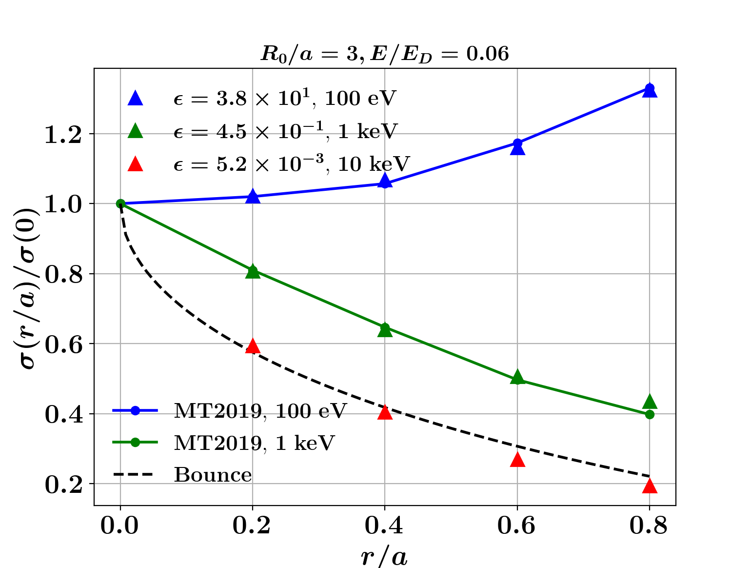
(a) Eulerian electric-field treatment

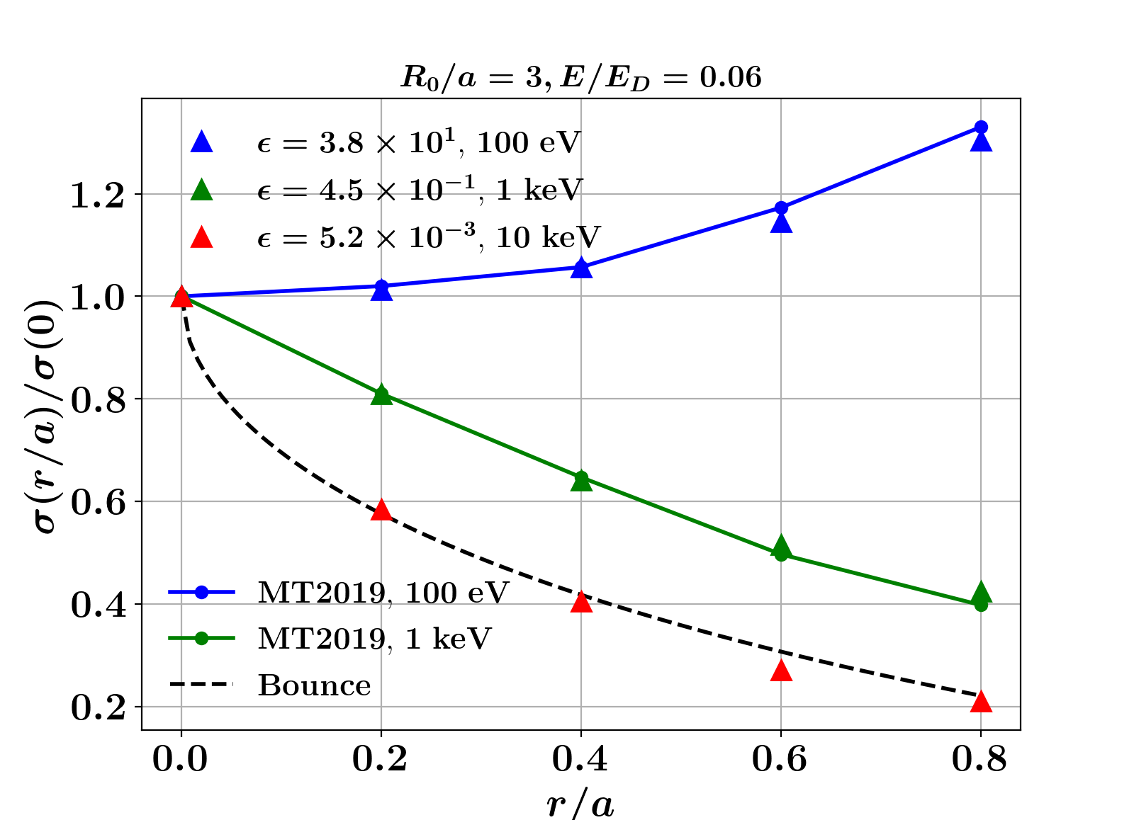
(b) Lagrangian electric-field treatment

Figure 8: Comparison of the relative change of Dreicer generation rates vs. the $r=0$ value along radius in the axisymmetric cylindrical tokamak geometry with results in Fig. 4 in Ref. [6], with the electric field treated (a) either on the mesh with $D^{*}=0.2$ or (b) in the orbit integral with $D^{*}=0.05$. The bounce-averaged solution is from Ref. [4]. Note that the asymptotic parameter $\epsilon$ in the left figure ranges from 38 to 0.005 depending on the plasma temperature, illustrating the need for a uniformly convergent algorithm. These plots demonstrate that the results are not only largely independent of the electric-field treatment, but also on the value of $D^{*}$ (provided it is chosen in the stable range).

The key result of this study is depicted in Fig. 8, which compares the relative Dreicer generation rates for various plasma temperatures as a function of plasma radius to the results in Ref. [6]. Both Lagrangian-$E$ and Eulerian-$E$ approaches demonstrate excellent agreement with published data for all plasma temperatures, illustrating the ability of the method to treat all relevant asymptotic regimes. In particular, it demonstrates that our implementation is not just asymptotic-preserving (i.e., able to capture the $\epsilon\rightarrow 0$ limit), but in fact uniformly convergent in $\Delta t/\epsilon$.

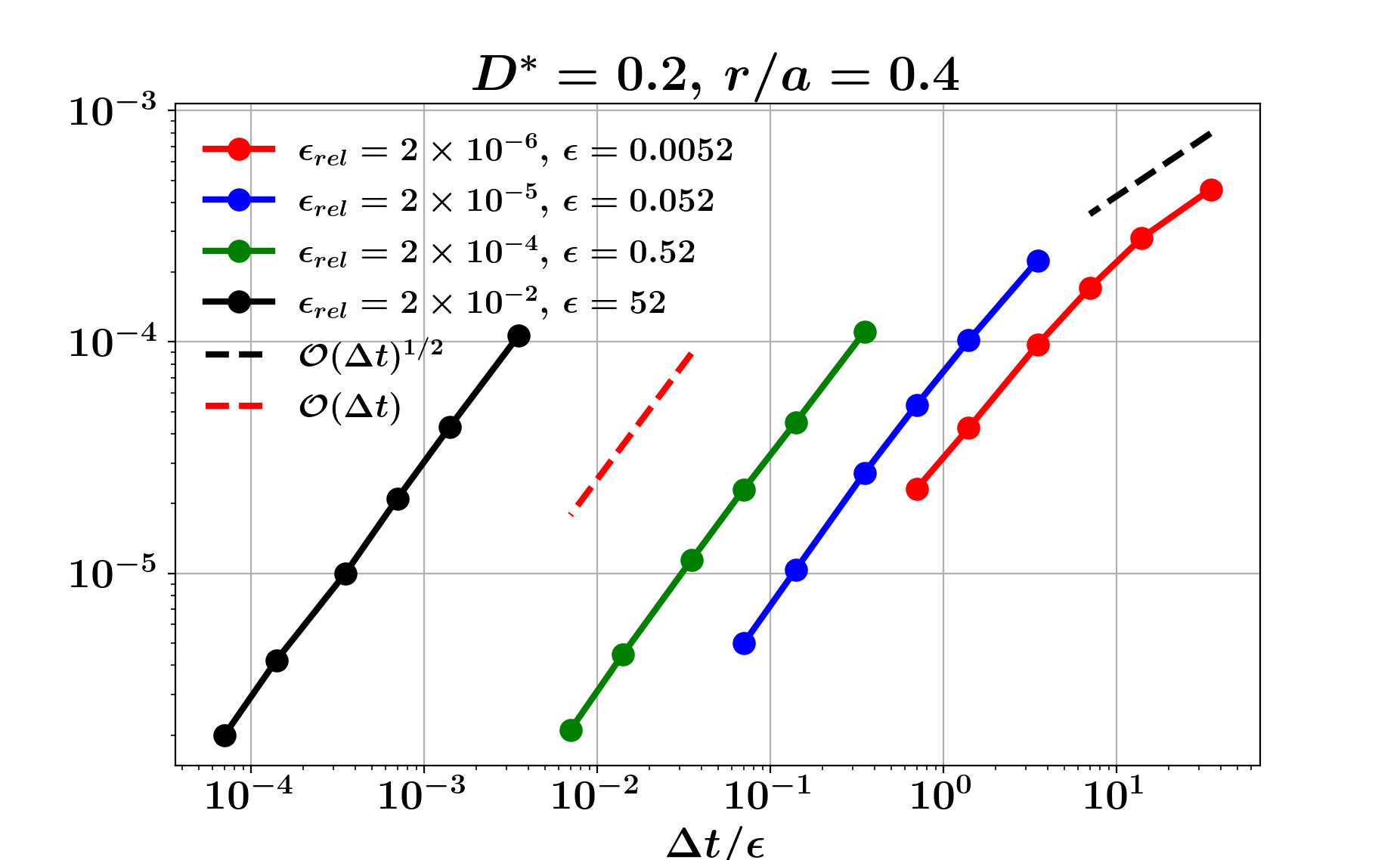
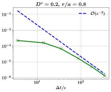
Figure 9: Convergence study results for the cylindrical tokamak 10 keV plasma in terms of $\Delta t/\epsilon$ showing first-order temporal convergence for $\Delta t/\epsilon$ small (left) and $\epsilon^{2}$ for $\Delta t/\epsilon$ large (right), with particular choices of $D^{*}$ and $r/a$ as indicated in the title figures. Results are obtained with the Eulerian electric-field treatment.

This point is further demonstrated in Fig. 9, where we show error convergence studies in terms of both $\Delta t$ and $\epsilon$ for the 10 keV case with an Eulerian-$E$ treatment. The error is computed as a volume-averaged root-mean-square of the solution difference,

$$\|f-f_{ref}\|_{2}=\left(\frac{{1}}{\pi L_{p_{\parallel}}L_{p_{\perp}}^{2}}\sum_{i=1}^{N_{\theta}}\sum_{j=1}^{N_{\parallel}}\sum_{k=1}^{N_{\perp}}(f-f_{ref})^{2}p_{\perp}\Delta p_{\parallel}\Delta p_{\perp}\Delta\theta\right)^{1/2},$$

where $f_{ref}$ is the reference solution. The figure on the left was obtained for various $\epsilon$ values by varying the time step $\Delta t$. Errors for a given $\epsilon$ are computed at a final time that was 10 times the largest time step, and are measured with respect to a reference solution employing the same mesh resolution and a timestep that is an order of magnitude smaller than the smallest timestep considered. Errors in the figure on the right employ a single time step of $\Delta t=0.2\tau_{c}^{th}$, and $\epsilon=(5.2,10.45,20.9,52.2,130.6,522.7)\times 10^{-4}$. Errors are computed with respect to a reference solution obtained on the same mesh and timestep and $\epsilon=5.2\times 10^{-5}$. In both these figures, $\epsilon$ is varied by artificially changing the plasma radius $R_{0}$ for constant plasma temperature. Figure 9-left demonstrates that the algorithm is first-order accurate in $\Delta t$ as long as $\Delta t/\epsilon<\mathcal{O}(1)$, while Fig. 9-right shows that the convergence of the algorithm in the large $\Delta t/\epsilon$ asymptotic regime scales as $\epsilon^{2}$. These results confirm the analysis in Sec. 3.5.

Table 1: Relative Dreicer growth rate $\sigma/\sigma(0)$ at $r/a=0.6$ for various temperatures and $D^{*}$ values using the Eulerian-$E$ treatment, demonstrating insensitivity of this physical figure of merit to $D^{*}$ .

$D^{*}$	0.2	1.0
100 eV	1.157	1.160
1 keV	0.501	0.507

A desirable property is the insensitivity of the physics to the numerical parameter $D^{*}$. Figure 8 already has established that the Dreicer generation rate is largely insensitive to the choice of $D^{*}$, provided that it is chosen in the stable range. Additional proof is provided in Table 1, where we list the relative Dreicer growth rates for two values of $D^{*}$ and two temperatures using the Eulerian-$E$ treatment, demonstrating the insensitivity of this physical figure of merit to $D^{*}$.

5.2.3 Scalability and performance of algorithm

Table 2 lists the wall-clock time (WCT) per time step for the hot (10 keV) plasma at $r/a=0.4$ case with the Eulerian-$E$ treatment, using both global and local interpolation methods in the orbit integration. The hot case is representative to assess the impact of the Lagrangian step on performance, as $\epsilon\ll 1$ and orbits are long. The local interpolation scheme is about twice faster than the global scheme for all grids and processor counts considered, confirming earlier 0D-2P observations. The Table suggests that the local interpolation scheme will outperform the global scheme by a larger factor as the mesh is refined, which is expected. The WCT scales linearly with the number of degrees of freedom and inversely proportional to the processor count, demonstrating an optimal, scalable semi-Lagrangian algorithm. This is expected, as both the Eulerian and the Lagrangian steps are themselves scalable and optimal. The excellent parallel and algorithmic scalability of the Eulerian implicit collisional solver has been documented in Ref. [14]. The Lagrangian step is also expected to be optimal as it integrates one orbit per Eulerian mesh point, and the cost per orbit scales as $\Delta t\sqrt{D^{*}}/\epsilon$, independently of mesh refinement. The results in the Table also demonstrate that our implementation exhibits strong parallel scalability.

Table 2: Total wall-clock time (WCT, in seconds per $\Delta t)$ of the semi-Lagrangian algorithm for the hot (10 keV) case at $r/a=0.4$ using the Eulerian-$E$ treatment with both local and global interpolation strategies.

Grid ($N_{\theta}\times N_{p_{\parallel}}\times N_{p_{\perp}}$)	MPI tasks	Grid per MPI task	WCT local int.	WCT global int.	WCT ratio
Spatial grid-refinement study
$8\times 256\times 128$	512	$2\times 16\times 16$	2.7	4.8	1.77
$16\times 256\times 128$	512	$4\times 16\times 16$	4.9	9.5	1.93
$32\times 256\times 128$	512	$8\times 16\times 16$	9.7	18.7	1.93
Momentum space grid-refinement study
$32\times 128\times 64$	512	$2\times 16\times 16$	2.3	4.4	1.91
$32\times 256\times 128$	512	$8\times 16\times 16$	9.7	18.7	1.93
$32\times 512\times 256$	512	$32\times 16\times 16$	44.0	88.6	2.01
Strong parallel scalability study
$32\times 256\times 128$	128	$8\times 32\times 32$	34.5	67.3	1.95
$32\times 256\times 128$	256	$8\times 32\times 16$	17.7	34.3	1.94
$32\times 256\times 128$	512	$8\times 16\times 16$	9.7	18.7	1.93

6 Conclusions

We have proposed an asymptotic-preserving, uniformly convergent semi-Lagrangian numerical scheme for the 2D-2P relativistic collisional drift-kinetic equation (rDKE). The approach is based on a Green’s function reformulation of the hyperbolic transport component, which leads to a practical numerical scheme after suitable approximations of quantifiable accuracy impact. The scheme employs operator splitting to deal with collisional sources (and perhaps others), which avoids iteration of the stiff hyperbolic component without spoiling the asymptotic properties. The collisional step considers the full complexity of relativistic Fokker-Planck collisions and reuses the scalable and accurate strategy proposed in Ref. [14]. It can be run either in linearized or in nonlinear mode. The transport step consists of orbit integrals (lending the approach the semi-Lagrangian character), one per mesh point, using analytically derived kernels with given fields. Since one orbit is spawned per Eulerian mesh point, the cost of the Lagrangian step scales linearly with the number of unknowns, rendering the overall semi-Lagrangian algorithm both scalable and optimal. By providing targeted dissipation in the Lagrangian kernels, the method is self-conditioning, automatically projecting the solution to the slow asymptotic manifold when the asymptotic regime warrants it. For $\epsilon\ll 1$, the method gives a consistent solution to the limit problem, the so-called bounced-averaged Fokker-Planck equation. Unlike earlier studies for stiff hyperbolic transport [15, 16], our approach does not require either dimension or variable augmentation, or iteration in the stiff hyperbolic component. We demonstrate by analysis and numerical examples in realistic geometries that the scheme is first-order accurate in $\Delta t$ for $\Delta t<\epsilon$, and second-order accurate in $\epsilon$ for $\Delta t>\epsilon$. We have successfully verified the approach against published results on Dreicer runaway electron generation in axisymmetric cylindrical tokamak geometries for various plasmas temperatures [6], spanning all regimes of interest in $\epsilon$ and demonstrating the capabilities of the scheme.

While our implementation so far is limited to 2D configurations with nested flux surfaces, the approach itself features no such limitation, opening the possibility of the multiscale simulation of runaway electron dynamics in arbitrary 3D magnetic field topologies with full collisional physics. Future work will explore such an extension, as well as the inclusion of additional physics such as radiation forces, knock-on collisions, etc.

Appendix A Relativistic bounce-averaging operator

In the relativistic case, the Jacobian of the transformation from ($p_{\parallel},p_{\perp}$) to ($\mathcal{E}=mc^{2}\gamma-e\Phi,\mu$) is:

$$\mathcal{J}=\det\left[\frac{\partial(\mathcal{E},\mu)}{\partial(p_{\parallel},p_{\perp})}\right]=\frac{p_{\parallel}p_{\perp}}{m^{2}\gamma B(\mathbf{x})}.$$

Therefore, by the transformation of probability, $fp_{\perp}dp_{\perp}dp_{\parallel}=gd\mathcal{E}d\mu$, we have:

$$g(\mathcal{E},\mu)=\frac{m^{2}B\gamma}{p_{\parallel}}f(\mathbf{x},p_{\parallel},p_{\perp}).$$

Noting that, along a ($\mathcal{E},\mu$) orbit, the arc-length obeys:

$$ds=\frac{p_{\parallel}}{\gamma m}d\tau,$$

we find:

$$g(\mathcal{E},\mu)\left.\frac{ds}{B}\right|_{\mathcal{E},\mu}=mf\left.d\tau\right|_{\mathcal{E},\mu}\Rightarrow g(\mathcal{E},\mu)=\left\langle f\right\rangle_{\mathcal{E},\mu}=m\frac{\oint_{\mathcal{E},\mu}fd\tau}{\oint_{\mathcal{E},\mu}\frac{ds}{B}},$$

which defines the relativistic bounce-averaging operator sought.

Appendix B Local spline interpolation procedure

To perform second-order local interpolation at a point $(x,y,z)$ in our (non-uniform) logical mesh, we first identify the surrounding 27-point ($3\times 3\times 3)$ stencil $(x_{i},y_{j},z_{k})$ that encapsulates said phase-space location, and express the interpolated value sought as:

$$p=\sum_{i=0}^{2}\sum_{j=0}^{2}\sum_{k=0}^{2}N_{i,j,k}(x,y,z)p_{i,j,k},$$

where $N_{i,j,k}(x,y,z)$ is the shape function centered at the node $(x_{i},y_{j},z_{k})$ (with specific properties, as explained below), and $p_{i,j,k}$ are the nodal values of the function we wish to interpolate. Shape functions have unit value at the node in which they are centered and vanish at all other nodes. Also, they form a partition of unity (the sum of all shape functions at any interpolated point $(x,y,z)$ is equal to one). For example, the shape function at $(x_{2},y_{2},z_{2})$ is given by:

$$N_{2,2,2}(x,y,z)=\frac{{(x-x_{1})(x-x_{0})}(y-y_{1})(y-y_{0})(z-z_{1})(z-z_{0})}{{(x_{2}-x_{1})(x_{2}-x_{0})}(y_{2}-y_{1})(y_{2}-y_{0})(z_{2}-z_{1})(z_{2}-z_{0})},$$

such that

$$N_{2,2,2}(x_{2},y_{2},z_{2})=1,$$

and

$$N_{2,2,2}(x_{i},y_{j},z_{k})=0,\qquad\mathrm{{for}\quad}i,j,k\neq 2.$$

Also,

$$\sum_{i=0}^{2}\sum_{j=0}^{2}\sum_{k=0}^{2}N_{i,j,k}(x,y,z)=1$$

for arbitrary $(x,y,z)$.

References

- [1] L. C. Woods, Theory of tokamak transport: new aspects for nuclear fusion reactor design. John Wiley & Sons, 2006.
- [2] J. Connor and R. Hastie, “Relativistic limitations on runaway electrons,” Nuclear fusion, vol. 15, no. 3, p. 415, 1975.
- [3] A. Stahl, M. Landreman, O. Embréus, and T. Fülöp, “Norse: A solver for the relativistic non-linear fokker–planck equation for electrons in a homogeneous plasma,” Computer Physics Communications, vol. 212, pp. 269–279, 2017.
- [4] E. Nilsson, J. Decker, Y. Peysson, R. S. Granetz, F. Saint-Laurent, and M. Vlainic, “Kinetic modelling of runaway electron avalanches in tokamak plasmas,” Plasma Physics and Controlled Fusion, vol. 57, no. 9, p. 095006, 2015.
- [5] Z. Guo, C. J. McDevitt, and X.-Z. Tang, “Phase-space dynamics of runaway electrons in magnetic fields,” Plasma Physics and Controlled Fusion, vol. 59, no. 4, p. 044003, 2017.
- [6] C. McDevitt and X.-Z. Tang, “Runaway electron generation in axisymmetric tokamak geometry,” EPL (Europhysics Letters), vol. 127, no. 4, p. 45001, 2019.
- [7] C. J. McDevitt, Z. Guo, and X.-Z. Tang, “Spatial transport of runaway electrons in axisymmetric tokamak plasmas,” Plasma Physics and Controlled Fusion, vol. 61, no. 2, p. 024004, 2019.
- [8] R. Harvey, V. Chan, S. Chiu, T. Evans, M. Rosenbluth, and D. Whyte, “Runaway electron production in DIII-D killer pellet experiments, calculated with the CQL3D/KPRAD model,” Physics of Plasmas, vol. 7, no. 11, pp. 4590–4599, 2000.
- [9] J. Decker, E. Hirvijoki, O. Embreus, Y. Peysson, A. Stahl, I. Pusztai, and T. Fülöp, “Numerical characterization of bump formation in the runaway electron tail,” Plasma Physics and Controlled Fusion, vol. 58, no. 2, p. 025016, 2016.
- [10] M. Landreman, A. Stahl, and T. Fülöp, “Numerical calculation of the runaway electron distribution function and associated synchrotron emission,” Computer Physics Communications, vol. 185, no. 3, pp. 847–855, 2014.
- [11] L. Hesslow, O. Embréus, G. J. Wilkie, G. Papp, and T. Fülöp, “Effect of partially ionized impurities and radiation on the effective critical electric field for runaway generation,” Plasma Physics and Controlled Fusion, vol. 60, p. 074010, jun 2018.
- [12] A. J. Brizard and A. A. Chan, “Nonlinear relativistic gyrokinetic vlasov-maxwell equations,” Physics of Plasmas, vol. 6, no. 12, pp. 4548–4558, 1999.
- [13] B. J. Braams and C. F. Karney, “Differential form of the collision integral for a relativistic plasma,” Physical review letters, vol. 59, no. 16, p. 1817, 1987.
- [14] D. Daniel, W. T. Taitano, and L. Chacón, “A fully implicit, scalable, conservative nonlinear relativistic fokker–planck 0d-2p solver for runaway electrons,” Computer Physics Communications, vol. 254, p. 107361, 2020.
- [15] N. Crouseilles, M. Lemou, and F. Méhats, “Asymptotic preserving schemes for highly oscillatory vlasov–poisson equations,” Journal of Computational Physics, vol. 248, pp. 287–308, 2013.
- [16] B. Fedele, C. Negulescu, and S. Possanner, “Asymptotic-preserving scheme for the resolution of evolution equations with stiff transport terms,” Multiscale Modeling & Simulation, vol. 17, no. 1, pp. 307–343, 2019.
- [17] R. Harvey and M. McCoy, “The CQL3D Fokker-Planck code,” in Proceedings of the IAEA Technical Committee Meeting on Simulation and Modeling of Thermonuclear Plasmas, pp. 489–526, 1992.
- [18] J. Decker and Y. Peysson, “DKE: A fast numerical solver for the 3d drift kinetic equation,” Euratom-CEA Report No. EUR-CEA-FC-1736, 2004.
- [19] Y. Petrov and R. W. Harvey, Benchmarking the fully relativistic collision operator in CQL3D. CompX report CompX-2009-1, 2009.
- [20] L. Chacon, D. del Castillo-Negrete, and C. D. Hauck, “An asymptotic-preserving semi-lagrangian algorithm for the time-dependent anisotropic heat transport equation,” Journal of Computational Physics, vol. 272, pp. 719–746, 2014.
- [21] H. Dreicer, “Electron and ion runaway in a fully ionized gas. i,” Physical Review, vol. 115, no. 2, p. 238, 1959.
- [22] P. Bhatnagar, E. Gross, and M. Krook, “A model for collision processes in gases. i. small amplitude processes in charged and neutral one-component systems,” Phys. Rev. Let., vol. 94, no. 3, pp. 511–525, 1954.
- [23] A. C. Hindmarsh, “ODEPACK, a systematized collection of ODE solvers,” in Scientific Computing (R. S. Stepleman, ed.), pp. 55–64, North-Holland, Amsterdam, 1983.
- [24] R. M. Kulsrud, Y.-C. Sun, N. K. Winsor, and H. A. Fallon, “Runaway electrons in a plasma,” Physical Review Letters, vol. 31, no. 11, p. 690, 1973.
- [25] J. Huba, “NRL Plasma Formulary 2009,” tech. rep., NAVAL RESEARCH LAB WASHINGTON DC BEAM PHYSICS BRANCH, 2009.