Orienting Point Clouds with Dipole Propagation

Abstract.

Establishing a consistent normal orientation for point clouds is a notoriously difficult problem in geometry processing, requiring attention to both local and global shape characteristics. The normal direction of a point is a function of the local surface neighborhood; yet, point clouds do not disclose the full underlying surface structure. Even assuming known geodesic proximity, calculating a consistent normal orientation requires the global context. In this work, we introduce a novel approach for establishing a globally consistent normal orientation for point clouds. Our solution separates the local and global components into two different sub-problems. In the local phase, we train a neural network to learn a coherent normal direction per patch (i.e., consistently oriented normals within a single patch). In the global phase, we propagate the orientation across all coherent patches using a dipole propagation. Our dipole propagation decides to orient each patch using the electric field defined by all previously orientated patches. This gives rise to a global propagation that is stable, as well as being robust to nearby surfaces, holes, sharp features and noise.

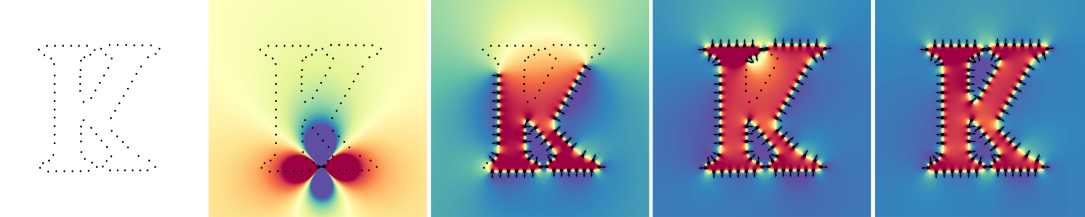
Figure 1. An iterative dipole propagation correctly predicts a consistent normal orientation from an unstructured point cloud.

1. Introduction

Deep learning has been used to successfully synthesize point clouds for shape generation [Achlioptas et al., 2018; Li et al., 2018c; Yang et al., 2019; Cai et al., 2020], shape completion [Yuan et al., 2018; Wang et al., 2020], and up-sampling/consolidation [Yu et al., 2018a, b; Yifan et al., 2019b; Metzer et al., 2020]. However, since standard loss functions (e.g., adversarial or Chamfer) do not trivially enable normal regression, these methods do not generate a globally consistent normal orientation. In addition, auxiliary information needed to reconstruct a correct normal orientation (e.g., visibility direction) from various scanning modalities may be lost in processing (registration/re-sampling/editing) scanned point cloud data. Yet, a consistent normal orientation for point clouds is a pre-requisite for many techniques in computer graphics and vision, for example: surface reconstruction [Kazhdan, 2005; Kazhdan et al., 2006; Kazhdan and Hoppe, 2013], signing distance-fields, voxelizing volumes (i.e., tetrahedralization), triangulating point sets, determining inside/outside information, and rendering point sets. Thus, geometric computation is highly limited for point clouds that lack a consistent normal orientation, either struggling or failing completely to produce a meaningful solution.

Establishing a consistent normal orientation for point clouds is a notoriously difficult problem in geometry processing, requiring attention to both local and global attributes. The normal direction of a point is a function of the local surface neighborhood. Yet, since point sets do not represent the underlying surface structure, the definition of local surface neighborhoods on point clouds is ill-defined. As such, point normals are estimated based on Euclidean neighborhoods, which do not necessarily imply geodesic proximity (especially in regions with nearby surfaces, non-convex structures and cavities).

Even when geodesic information is given, calculating a globally consistent normal orientation is non-trivial, and requires global context. Notably, when examining a flat patch from a shape in isolation, e̊stablishing whether the surface plane points outward or inward is ambiguous (see Figure \ref{fig:local_uncertain}). Propagation techniques propose overcoming this ambiguity by starting with one correctly oriented point normal and diffusing its orientation across the entire shape [Hoppe et al., 1992]. However, such a propagation technique assumes smoothness (i.e., that nearby normals are similar), leading to undesirable solutions in the case of sharp features, nearby surfaces, and noise. Moreover, the orientation accuracy is sensitive to the propagation neighborhood size; while a large neighborhood is desirable to smooth out noise and outliers, it also risks erroneously including nearby surfaces. A notably undesirable attribute of such techniques is their greediness, since during iterative propagation one incorrectly oriented patch degrades all subsequent propagation steps.

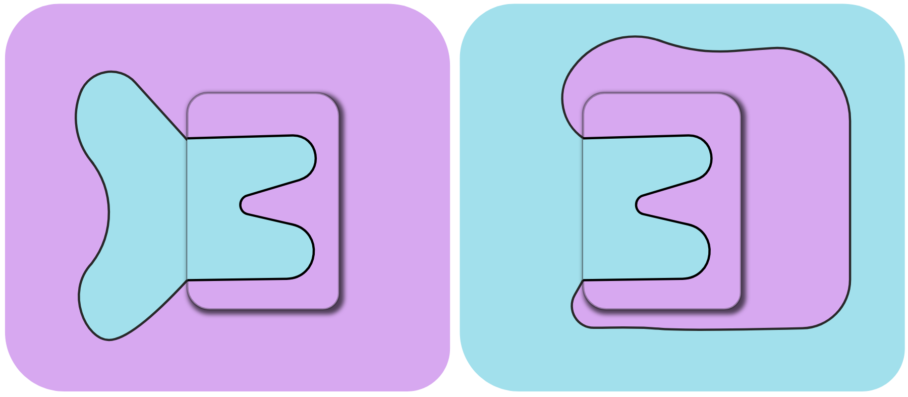
Figure 2. The global orientation from a local patch is ill-defined. The exact same blue or purple regions in a patch can represent either inside or outside information, depending on the global context.

In this work, we introduce a new approach for orienting point clouds. We split the orientation problem into two sub-problems, local and global, which are solved sequentially. We partition the point cloud into local patches, and learn a coherent normal direction per patch using a neural network, such that all normals are consistently pointing either inside or outside the surface. Specifically, we aim to detect and flip normals that do not agree with the majority direction of all input point normals in the same patch. Note that locally there is no sense of correctness, thus we only require patch consistency in the majority direction of the input normals. Instead of propagating the global orientation across individual points, we propagate across coherent patches. We introduce a dipole propagation that solves global orientation by iteratively placing electric dipoles across each coherent patch. This incrementally builds a global electric field, where each new patch is oriented using the electric field of all previously oriented patches (see Figure 1).

In patches with nearby surfaces, non-convex structures, noise, and cavities, calculating a coherent normal direction is challenging and usually requires pre-defined heuristics, e.g., for sharp features [König and Gumhold, 2009] or thin surfaces [Xu et al., 2018] (see Figure 3). Yet, this task is well suited for a neural network which can automatically learn a data-driven prior. To this end, we train a neural network to estimate a coherent normal direction using self-supervision (points sampled from watertight meshes). Specifically, the network learns to classify whether each input point normal agrees with the majority direction of all input point normals in the same patch. The network-predicted probabilities are used to flip inconsistent normals within each patch, as well as guide the global dipole propagation.

Our dipole propagation calculates a consistent global orientation by iteratively propagating the correct orientation across all coherent patches using a global objective. Notably, the entire set of previously oriented patches are used to determine the orientation of the next patch. Unlike MST-based propagation [Hoppe et al., 1992] which only considers the previous (adjacent) orientation, our dipole propagation considers the orientation of all previously oriented patches. Specifically, we progressively build a global electric field, which is used to orient each new patch based on the network-predicted confidence scores as well as the interaction between the electric field of all previously oriented patches. By visiting all patches (and flipping them, where appropriate), we obtain a double layer potential [Folland, 1995] whose scalar value at any point in space indicates inside or outside the shape surface. This electric potential was also referred to as the winding number for oriented point clouds [Barill et al., 2018].

A few inconsistently oriented points only degrades the electric field locally (also noted by [Barill et al., 2018]), leading to a dipole propagation which is robust to noise and outliers. If small errors exist (e.g., from the neural network), they do not accumulate, which enables converging to a desirable solution in spite of the noise. Moreover, after dipole propagation is complete, we leverage the global electric field and diffuse it across all points to flip any normals incorrectly estimated by the network. Another advantage of our dipole formulation enables building an electric field from known normal orientations, which is useful when part of the input point cloud contains known normals (e.g., in point cloud upsampling).

We demonstrate the effectiveness of our technique on a variety of different 3D point clouds. We show that our neural patch coherency network can consistently orient unstructured point sets, even in the presence of noise, nearby surfaces, sparsely sampled regions, sharp features, and cavities. In our ablation studies, we show that our neural network improves dipole propagation speed and also accuracy. Moreover, we show the applicability of our approach to clouds generated from neural networks for shape generation, shape completion, and point cloud consolidation. Our strategy also scales to large point clouds, and we show results on clouds with over one million points. In our quantitative evaluations, we demonstrate on-par or improved performance relative to state-of-the-art methods for point cloud orientation.

\begin{overpic}[width=433.62pt]{figures/2D/baby_shark/baby_shark_comparison.jpg} \put(7.0,-4.3){{\color[rgb]{0,0,0}Input}} \put(28.0,-4.3){{\color[rgb]{0,0,0}Hoppe}} \put(54.0,-4.3){{\color[rgb]{0,0,0}König}} \put(75.0,-4.3){{\color[rgb]{0,0,0}Ours}} \end{overpic}

Figure 3. Starting with an input point cloud (left), the result of orientation via tangent plane normal propagation [Hoppe et al., 1992], or an improved version [König and Gumhold, 2009], both converge to an undesirable solution. Our dipole propagation is able to correctly orient each patch of coherently directed points, resulting in a desirable dipole electric potential (where blue is outside, and red is inside the surface).

2. Related Work

We first discuss techniques for cloud orientation, which we categorize as either surficial or volumetric. Surficial methods generally propagate the orientation information starting from a single point across the entire sampled surface. Volumetric methods aim to partition the space into inside/outside, where surface normals should point from inside to outside the surface. Then we discuss deep learning techniques for generating point clouds (i.e., point locations), for up-sampling/consolidation, shape generation, and shape completion. Indeed, using such synthesized clouds for downstream tasks will also require estimating point normals, and by extension, their orientation.

2.1. Normal Orientation Techniques

Surficial methods.

The pioneering work of Hoppe et al. [1992], introduced the paradigm of point normal orientation propagation via a minimum spanning tree (MST). An MST graph is built on the point cloud, where every edge between two points is assigned a weight based on the (absolute) similarity between their respective normals (later extended by Pauly et al. [2003] to weight distances based on an exponentially decaying function [Levin, 2004]). Starting with a single correctly oriented point normal, the orientation is propagated to nearby points across the MST graph. However, this technique is known to be highly sensitive to the choice of neighborhood size [Mitra and Nguyen, 2003], since a large neighborhood irons out noise, but risks including nearby surfaces. The MST paradigm is greedy and one incorrect orientation step degrades all subsequent propagation, as we demonstrate in our comparisons (Section 5). In contrast, our work uses a global criteria to robustly handle eventual inconsistencies by considering the orientation of all previously oriented patches.

Subsequent works proposed handling unique failure cases of the above paradigm [Guennebaud and Gross, 2007; Huang et al., 2009; Xu et al., 2018]. For example, in the case of sharp features, Xie et al. [2003] propose a multi-seed propagation that initially avoids sharp features, resulting in multiple oriented patches touching at sharp corners, which are consistently oriented in a second phase. This was later improved and extended by König and Gumhold [2009], to flip normals based on the smoothness of a Hermite curve. However, our experiments demonstrate that a single mistake during propagation using König and Gumhold [2009] will result in a large incorrectly oriented region due to the greediness of MSTs (see Figure 4).

\begin{overpic}[width=433.62pt]{figures/005_hands_comparison.png} \put(8.0,-4.0){{\color[rgb]{0,0,0}König}} \put(45.0,-4.0){{\color[rgb]{0,0,0}PCP-Net}} \put(80.0,-4.0){{\color[rgb]{0,0,0}Ours}} \end{overpic}

Figure 4. Normal orientation estimation, where angle errors are visualized in a heat map. The MST-based technique of [2009] fails at some point in the propagation, which results in a large region of accumulated errors. PCP-Net [2018] uses only local information, which leads to a sub-optimal solution.

In order to mitigate errors from greedy MSTs, Schertler et al. [2017] propose using a global optimization to fix errors, which can also handle large point clouds. Our experiments show that Schertler et al. [2017] struggles with noise and high-frequency details, and is much slower to compute on large point clouds. For example, in Figure 6 shows the favorable results of our method on a point cloud of over 1 million points which took 13 minutes to run, compared to 90 minutes for Schertler et al. [2017]. Jakob et al. [2019] suggested propagating the orientation through edge collapse operations, with hand-crafted heuristics for each edge energy, as an alternative approach to MST propagation for approximating the global minimum.

To try and construct a more global criterion, Seversky et al. [2011] introduces the use of harmonic functions (built from a predefined point cloud laplacian) for propagating orientation over the MST. Similar to the previous approaches, MST propagation suffers from cumulative error, and in addition the Laplacian operator for point clouds will inevitability be unstable when two surfaces are close, due to lack of geodesic connectivity, and we show an example of this problematic case in the supplementary material. We also show that our approach can robustly handle the same case.

\begin{overpic}[width=433.62pt]{figures/006_hands_comparison_recon.png} \put(8.0,-4.0){{\color[rgb]{0,0,0}Signing}} \put(45.0,-4.0){{\color[rgb]{0,0,0}König}} \put(80.0,-4.0){{\color[rgb]{0,0,0}Ours}} \end{overpic}

Figure 5. Reconstruction results directly estimated by signing [Mullen et al., 2010], where as the estimated normal orientation of König [König and Gumhold, 2009] and our dipole-propagation are used as input to PSR [Kazhdan et al., 2006].

Volumetric methods.

An alternative paradigm aims to partition the 3D space into inside/outside, where surface normals should point from inside to outside the surface. Mello et al. [2003] propose an adaptively subdivided tetrahedral volume to calculate the in/out function from an unoriented point set (see comparison in Figure 5, where close surfaces of the index and middle finger are incorrectly lumped together). Xie et al. [2004] grow active contours to carve out inside/outside. Chen et al. [2010] use binary orientation trees to determine inside/outside using point set visibility [Katz et al., 2007]. Some methods reconstruct a signed function from unoriented points using a variational formulation [Walder et al., 2005; Huang et al., 2019]; yet they are limited to small point clouds, since their computational complexity does not scale well with resolution (see a comparison on 500 points in Figure 16). Whereas we demonstrate that our method scales point clouds with 10 million points. Generally, volumetric methods struggle to deal with open surfaces and large holes, whereas surficial methods can struggle on sharp features and/or a greedy local objective (see Figures 3, 4, 6, and 17).

\begin{overpic}[width=433.62pt]{figures/007_dragon_results.png} \put(8.0,-4.0){{\color[rgb]{0,0,0}QPBO}} \put(45.0,-4.0){{\color[rgb]{0,0,0}Hoppe}} \put(80.0,-4.0){{\color[rgb]{0,0,0}Ours}} \end{overpic}

Figure 6. Consistent normal orientation results on a scanned point cloud containing over 1 million points (errors visualized using a heat map). QPBO [2017] contains the most error, and took 90 minutes. Hoppe [Hoppe et al., 1992] contains less error, and took 2 minutes. Our method has fewest errors and took 13 minutes to run.

In this work, unlike previous methods, we present a technique for point cloud orientation that leverages the power of data-driven learning with a proposed dipole propagation. Our dipole propagation defines a global objective function, and the propagation at each iteration becomes significantly less greedy, as we consider all previously oriented points. Our approach can be viewed as taking the best of the surficial approaches (operating directly on the surface points) and volumetric approaches (providing an inside / outside segmentation as a byproduct of the electric dipole field).

2.2. Neural Point Cloud Generation

There has been a rising interest in extending the success of deep neural networks to irregular domains. Pointnet [Qi et al., 2017a] pioneered the first neural network to directly consume point clouds (followed by several improved architectures [Qi et al., 2017b; Wang et al., 2019]), and demonstrated impressive results on discriminative tasks. This sparked interest in applying pointnet-like architectures to synthesize point clouds, for shape generation, shape completion, and up-sampling/consolidation. However, synthesizing a globally consistent normal orientation along with each point location is non-trivial. Specifically, standard loss functions (e.g., adversarial or Chamfer) do not provide point-to-point correspondence on the underlying surface, which prevents defining a ground-truth normal orientation for any given synthesized point.

Consolidation.

Deep learning techniques which generate point clouds for a downstream task (e.g., surface reconstruction) require some type of normal estimation / orientation on the synthesized point cloud. For example, Deep Geometric Prior (DGP) [Williams et al., 2019] learns to consolidate point clouds, which when used in combination with Poisson reconstruction [Kazhdan et al., 2006; Kazhdan and Hoppe, 2013], results in surface reconstruction. Yet, since DGP does not regress oriented point normals, normal orientation must be solved in a post-process before using Poisson reconstruction. EC-Net [Yu et al., 2018a] consolidates point clouds, specifically on sharp edges, and requires estimating the point normals for surface reconstruction using PCA, which are indeed unoriented. Multi-step progressive upsampling (MPU) [Yifan et al., 2019b] upsample point sets using a detail-driven deep neural network, which was demonstrated to improve surface reconstruction, which also requires normal and orientation estimation. Subsequently, PU-GAN [Li et al., 2019] proposed a generative adversarial network for upsampling point clouds, which also demonstrated improvement in surface reconstruction quality in sparse and non-uniform inputs. Self-sampling [Metzer et al., 2020] proposed consolidating point clouds using a single example, and required estimating the point normals in a post-process. Thus, employing deep learning based point consolidation / up-sampling techniques [Yu et al., 2018b], requires normal estimation and orientation estimation for downstream tasks. PCP-Net [Guerrero et al., 2018] proposed learning point properties (e.g., oriented normals and curvature) from local patches. However, since normal orientation is a global problem (i.e., Figure 2), using only local information from patches leads to a sub-optimal solution (see Figure 4).

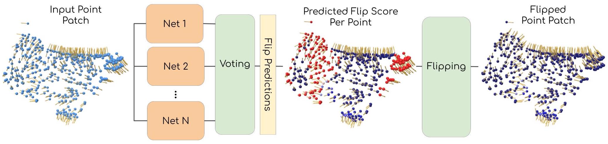
Figure 7. Coherent patch neural network. An input patch (point locations and estimated normals using Jets [Cazals and Pouget, 2005]), is input to an ensemble of individual point networks which predict and vote on the probability that each point normal in the patch should be flipped. Point probabilities colored using a heat map, where high probabilities are red. The network is trained using supervised learning, where the network is encouraged to predict a high flip probability for point normals which do not agree with the majority direction the input normals. After flipping the normals according to the network-predicted probabilities, we obtain a coherent normal orientation per-patch.

Denoising.

Many deep learning techniques have been presented for point cloud denoising [Hermosilla et al., 2019; Luo and Hu, 2020; Lang et al., 2020]. Indeed, using the denoised cloud requires estimating normals based on the new point locations, necessitating normal orientation. Learning-based surface splatting was presented in [Yifan et al., 2019a], and when denoising clouds the normals were computed using [Hoppe et al., 1992]. PointCleanNet [Rakotosaona et al., 2020] trained a neural network to map noisy points to clean ones and then demonstrated surface reconstruction using normals estimated using Meshlab. Huang et al. [2020] proposed non-local part-aware deep neural networks for denoising point locations, and demonstrated applicability to surface reconstruction. Pistilli et al. [2020] developed a graph-convolutional neural network for denoising point clouds, which improved unoriented normal estimation using off-the-shelf tools.

Synthesis.

Deep learning has been used to synthesize point clouds in a variety of generative tasks. For example, in shape completion, neural networks are trained to synthesize points in missing regions[Yuan et al., 2018; Gurumurthy and Agrawal, 2019; Sarmad et al., 2019; Tchapmi et al., 2019; Wang et al., 2020; Wen et al., 2020; Liu et al., 2020]. Another body of works generate 3D point clouds from a single-view (i.e., RGB image) [Fan et al., 2017; Jiang et al., 2018]. A wealth of deep learning techniques for shape generation using unstructured point clouds have been proposed [Achlioptas et al., 2018; Yang et al., 2019; Cai et al., 2020]. A popular technique for generating point clouds is through auto-encoders [Li et al., 2018b; Yang et al., 2018; Groueix et al., 2018; Liu et al., 2019; Zhao et al., 2019]. PC-GAN [Li et al., 2018c] presented a technique for synthesizing point clouds using generative adversarial networks. PointGrow [Sun et al., 2020] proposed an autoregressive framework for generating each point recurrently. PointGMM [Hertz et al., 2020] predicts a mixture of Gaussians which can be sampled to obtain point locations.

Point-based neural generation techniques have focused primarily on regressing point locations, without normals. Yet, using synthesized clouds for downstream tasks will also require estimating point normals, and by extension, their orientation. Note that AtlasNet [Groueix et al., 2018] observed a drop in reconstruction performance when regressing point normals alongside locations, compared to only regressing point locations. This empirically demonstrates that using a Chamfer assignment for point normals does not guarantee the correct normal correspondence.

2.2.1. Deep Surface Reconstruction

Another line of works propose reconstructing 3D surfaces directly from point clouds. DeepSDF [Park et al., 2019] learns to generate a signed distance function (SDF) from an input point cloud. The zero level set of the SDF can be used to reconstruct an oriented surface, as well as produce oriented normals for the input points by back-propagating through the SDF network. The authors describe that while training on meshes, they choose the ground truth orientation of the normals based on cameras placed around the object, and discarded shapes where the orientation was ambiguous. Point2Mesh [Hanocka et al., 2020] reconstructs a watertight mesh from a point cloud by optimizing a MeshCNN [Hanocka et al., 2019] network to deform an initial mesh to shrink wrap the input point cloud. This work can utilize normal information if available, but also demonstrated results on point sets without normal orientation.

3. Overview

Our technique consists of two parts, first a local and then a global component. In the local phase, we partition the shape into local patches and train a neural network to estimate a coherent normal orientation per patch. In the second phase, we use the network confidence scores to guide a dipole propagation to globally orient normals across all coherent patches.

Coherent Neural Patch Orientation.

In the first phase, we partition the shape into non-overlapping patches and calculate the normal for each point in the patch: using Jets [Cazals and Pouget, 2005], where the normal direction is initialized by pointing away from center of mass. The network receives as input a list of point locations and normals, and learns to predict a flip probability per-point. Specifically, we train an ensemble of networks to predict a value between 0 ($=$ should be flipped) and 1 per-point, which vote on the final flip probability. During inference, we pass (unseen) patches to the trained network and flip each normal according to network-predicted probabilities, resulting in a coherently oriented patch. An illustration of this system is shown in Figure 7.

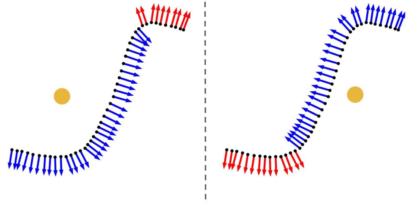
Figure 8. Different normal orientations based on the reference (yellow) point. The majority orientation is marked in blue, which is used to create the ground-truth labels during training (red = flip).

As mentioned previously, the global orientation is ambiguous for a single patch (see illustration in Figure 2). As such, the network objective is to predict flip probabilities such that the point normals in the input patch are coherently oriented, meaning that all normals are consistently pointing either inside or outside the surface. Since training on both possibilities is a non-smooth, ambiguous objective, we prescribe the correct coherent orientation based on the direction of the majority of the estimated point normal directions which is used as ground-truth (see Figures 8 and  12). The network estimated flip probabilities are also used to guide the dipole propagation to a desirable result.

Since calculating a consistent normal direction for flat or convex patches is trivial, the central challenge is estimating a consistent normal direction for patches with nearby surfaces, non-convex structures, sharp features and cavities. Yet, since these difficult cases occur less frequently we only train on patches that contain the difficult and ambiguous cases. This forces the network to focus on the rare cases that would otherwise be ignored (due to their low prevalence in the training data).

Dipole Propagation.

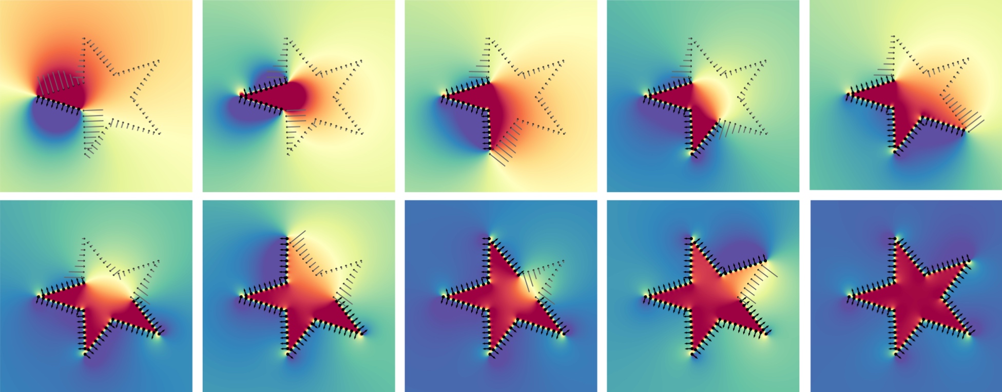
Figure 13. Iterative dipole propagation visualization. Starting with the first patch we place a dipole on every point in the patch. The electric potential dissipated by the dipoles shown in blue/red. We measure the interaction between the electric field (i.e., the gradient of the potential) and the normal of each point left to be oriented. The interaction is shown by a grey line with length proportional to the interaction value and direction of the unoriented normal. Note that the electric potential is only calculated for visualization purposes, and not necessary to calculate in practice.

We propagate the global normal orientation to all the coherently oriented patches in the shape using dipole propagation. We start by selecting a flat patch, and treat each point in the patch as an electric dipole with polarization that points in the normal direction, which generates an electric field. Then, we find the patch with the strongest (absolute) mutual dipole interaction with the current field, weighted by the network-predicted confidences. If the new patch interacts strongly in the opposite direction, we flip its orientation. We add the effects of the new patch to the total electric field by placing dipoles on each point in the new patch. We progressively build a global electric field, which is used to orient each new patch based on the electric field of all previously oriented patches. Once we have visited all patches (and possibly flipped them), we built an electric potential whose scalar value at any point in space indicates inside/outside the shape surface (see visualization in Figure 13). In the diffusion phase, we dissipate the final electric potential to fix possible errors made by the network. The neural network plays a crucial role, both in terms of generating coherently oriented patches and in terms of the flip probabilities which are used to correctly guide the propagation (see Figure 9.)

\begin{overpic}[width=433.62pt]{figures/014_network_diffusion.jpg} \put(6.0,-3.7){{\color[rgb]{0,0,0}w/o diffusion}} \put(39.0,-3.7){{\color[rgb]{0,0,0}w/o network}} \put(65.0,-3.7){{\color[rgb]{0,0,0}network + diffusion}} \end{overpic}

Figure 9. Normal orientation results without using diffusion (left), without using a neural network (middle), and both network and diffusion (right). A desirable normal orientation result relies on both the network and the diffusion phases. The neural network not only coherently orients each patch, but also provides confidence scores that are used during dipole propagation.

Note that the starting patching can have both possible orientations (all normals pointing inside or outside the surface). Upon completing propagation, we can flip the entire sign of the globally consistent normal orientation given a single correct point normal.

4. Method

4.1. Input Patch Data

We used supervised learning to learn a mapping between input patches (point locations and normal directions), to a flip probability per point. We generate supervised pairs of input patches and ground-truth flip labels for training. Training input patches are obtained by sampling point clouds (augmented with various types of noise) from watertight meshes, and then estimating the normals for each point in the patch using an off-the-shelf tool (e.g., PCA or Jets [Cazals and Pouget, 2005]). The corresponding ground-truth label of whether to flip each point’s normal is based on the majority normal orientation direction in the patch (see Figure 8).

Each point cloud is scaled to a unit cube and partitioned into patches corresponding to 3D cubical voxels (see Figure 10). After discarding empty voxel regions and merging patches smaller than $100$ points, we filter out planar patches (based on their smallest eigenvalue) since they are trivial to coherently orient (i.e., via a reference point on either side of the plane). We calculate normals for each point in the patch using an off-the-shelf algorithm and place each patch in a canonical axis using PCA.

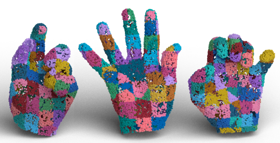
Figure 10. Visualization of our patch partitioning.

We use several forms of data augmentation to enrich the training set. During training, we flip each normal in the patch with probability $p$. This introduces uncorrelated local flip error that can be induced by noisy points, for example. We initially orient the estimated normals in each patch to point away from a single reference point. During inference, the reference point is the center of mass. However, to induce different types of training distributions, we randomly select different reference points within the bounding box containing the patch. This augmentation generates spatially correlated flip errors. For example, in a patch that contains a corner, changing the reference point to be above or inside the corner results in two different orientations for the perpendicular planes (see an example in Figure 8).

A strict definition of a coherently oriented patch has two valid possibilities (all normals pointing inside or outside the surface, where inside/outside cannot be defined at the patch-level). However, training on the best of the two options (i.e., min-distance) is non-smooth, and can oscillate between optima. In addition, this would enable the network to memorize spatial layouts of point patches (completely ignoring the input normal information), and always predict in the $+z$ direction, for example. Therefore, during training, we define a correct coherent orientation based on the direction of the majority of the estimated point normal directions. Orienting point normals in the same input patch using different reference points can lead to different majority normal directions, which results in a different ground-truth label (see Figure 8).

\begin{overpic}[width=260.17464pt]{figures/2D/baby_shark/flip_noise.jpg} \end{overpic}

Figure 11. Several inconsistently oriented points within a patch (5 out of 15), only degrades the electric potential locally. During dipole-propagation, if such local errors exist, e.g., from the neural network, they will not accumulate – which enables converging to a desirable solution (in spite of the noise).

4.2. Ensemble Training

We train an ensemble of point neural networks to coherently orient the non-planar patches, which contain the challenging cases of cavities, non-convex, and sharp feature regions. We use a PointCNN [Li et al., 2018a]-based network to predict a probability per point indicating whether it should be flipped. Specifically, the input to the network is a patch $\mathbb{P}\in\mathbb{R}^{N\times 6}$, represented as a collection of $N$ points containing the $xyz$ positions and a normal direction for each point. The output of the network $\in\mathbb{R}^{N\times 2}$ is two logits per point, which when passed to Softmax result in the $flip$ probability. The network is trained using supervision: the cross-entropy between the predicted probabilities and the ground-truth $flip$ label.

Each neural network in the ensemble can be trained with different network hyper-parameters and on different datasets. After training is complete, we average the probabilities from the different networks to obtain the final flip probability per-point. After flipping each normal according to the network-predicted probabilities the result is a coherently oriented patch.

Learning to predict a coherent normal orientation per point requires considering both nearby and far away points in the patch, which we address using an ensemble of multi-scale networks. The receptive-field of the neural network naturally dictates the amount of distant points. We obtain networks with a large receptive field by using an aggressive pooling strategy. Each network is composed of PointCNN convolution layers, FPS (farthest-point sampling) pooling, and feature interpolation unpooling [Qi et al., 2017b]. Our aggressive pooling strategy uses four FPS pooling layers, where each layer reduces the number of points by 40%. More details about our network architecture can be found in the supplementary material.

Despite the fact that the network may produce imperfect results, our system is well equipped to handle and eventually correct such errors. For example, during dipole propagation the electric potential is robust and only degrades locally when several points are inconsistently oriented (see Figure 11). In addition, our network predicts probabilities that we use to attenuate the effects of incorrect orientations. Finally, these lingering errors will be corrected in a second diffusion phase, which is explained in Section 4.3.4 (also visualized in Figure 9).

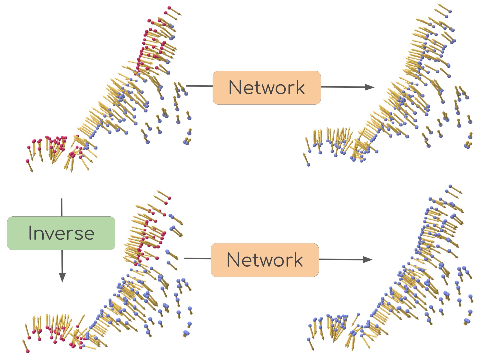
Figure 12. The network learns to coherently orient the input patch based on the direction of the majority of the input normals. When inverting the normal orientation on the input patch, the majority direction changes and the output orientation is similarly inverted.

4.3. Dipole Propagation

After the network has coherently oriented each patch in the input shape, we use dipole propagation to calculate a consistent global normal orientation across all the patches, iteratively. We progressively build a harmonic potential (Section 4.3.1) from all previously oriented patches, in order to infer the orientation of new patches. Starting from a planar patch (likely to contain least amount of coherent normal errors), we treat each point in the patch as an electric dipole with polarization that points in the normal direction $\hat{n}$. The dipoles generate an electric field, which is used to orient a new patch at each iteration. To choose which new patch to orient at each iteration, we measure the absolute value of the potential energy (Section 4.3.2) at each patch which has yet to be oriented, weighted by the flip probability scores from the network. The patch with the highest potential energy is chosen for orientation, and is flipped if the energy is negative, or remains if the energy is positive. The effect of the newly oriented patch is added to the current field, and the new field (result of the previous field and with newly oriented patch), is used to orient the rest of the patches in the same iterative manner. Our decision to treat points as electric dipoles is justified in the Poisson equation (Section 4.3.3), as well as the winding number [Barill et al., 2018], which we explain in more detail below. Finally, after all the patches have been oriented by the dipole propagation, we employ an extra diffusion step to fix small errors made by the network (Section 4.3.4).

$\vec{E}$ $\leftarrow$ $\mathbb{0}^{N\times 3}$

$P$ $\leftarrow$ flattest patch

$remaining$ $\leftarrow$ all patches except $P$

// The current field for all points not in $P$, denoted $\overline{P}$

$\vec{E}$[$\overline{P}$] += DipoleField (sources=$P$, measurements=$\overline{P}$)

while $remaining$ not empty do

       // Calculate interaction (Eq. (3)) for each patch

       i = argmax{ $\mid V_{j}\mid$ for j $\in$ $remaining$ }

       $P$ = $remaining$.Remove (i)

       if $V_{i}$ ¡ 0 then

             FlipPatch ($P$) // flips patch if interaction negative

            

       end if

      // add effect of new patch to the total field

       $\vec{E}$[$\overline{P}$] += DipoleField (sources=$P$, measurements=$\overline{P}$)

      

end while

// Diffusion Step

for point $k\in$ point cloud do

       // calculate interaction for every point $k$ in point cloud

       if $\hat{n}_{k}\cdot\vec{E}[k]<0$ then

             FlipPoint ($i$)

            

       end if

      

end for

Algorithm 1 Dipole Patch Propagation

4.3.1. Electric Dipole

In electrostatics, an electric dipole arises when two oppositely charged particles are brought close together. In our scenario, each oriented point normal is treated as an electric dipole, with polarization in the direction of the normal $\hat{n}_{i}$. The electric potential $u$ induced by such a dipole measured at point $\vec{r}$ is

(1) $$u(\vec{r})=\frac{c_{i}(\hat{n}_{i}\cdot\vec{r})}{4\pi\mid\vec{r}\mid^{3}},$$

where $c_{i}$ is the confidence score per point $i$ estimated by the neural network (proportional to the flip probability). This attenuates the effect of the points that the network is less confident about (flip probabilities close to $0.5$). The electric field is the gradient of $u$:

(2) $$\vec{E}=\vec{\nabla}u(\vec{r})=-\frac{3c_{i}(\hat{n}_{i}\cdot\hat{r})\hat{r}-c_{i}\cdot\hat{n}_{i}}{4\pi\mid\vec{r}\mid^{3}}.$$

Note that this is the electric field in physics up to a sign (in physics $\vec{E}=-\vec{\nabla}u(\vec{r})$). We drop the minus sign $\vec{E}=\vec{\nabla}u(\vec{r})$, since we want to orient points towards where the potential rises, rather than falls. Although this would imply that opposite charges repel (instead of attract), it is desirable in our orientation problem formulation.

4.3.2. Potential Energy

The potential energy between a patch and the currently dissipated field from previously oriented points is

(3) $$V_{patch}=\sum_{\hat{n_{i}}\in patch}c_{i}\cdot\hat{n_{i}}\cdot\vec{E}.$$

The neural network confidence $c_{i}$ mitigates possible errors made by the network, and encourages noisy patches to be oriented last.

4.3.3. Poisson Equation

The electric potential induced by such dipole is a solution to the Poisson equation, and has two important properties which are desirable for propagating normal orientation:

1. decreases with distance, and

2. negative on one side of the dipole and positive on the other.

While an electric dipole is not the only way to obtain the above properties, its key justification lies in the Poisson equation:

(4) $$\nabla^{2}u(\vec{r})=4\pi\rho(\vec{r}),$$

which characterizes the impact of the sources $\rho(\vec{r})$ (e.g., heat sources or charged particles) on the potential $u(\vec{r})$.

In our case, the sources are the oriented points and the potential is the scalar function $u(\vec{r})$. In this way, the electric potential from all oriented points is used to orient new points.

Since Equation (4) is linear and shift invariant, the superposition of sources $\rho_{i}(\vec{r})$ and solutions $u_{i}(\vec{r})$ is also a solution to the equations

(5) $$\nabla^{2}u_{total}(\vec{r})=\Sigma_{i}\nabla^{2}u_{i}(\vec{r})=\Sigma_{i}4\pi\rho_{i}(\vec{r})=4\pi\rho_{total}(\vec{r}).$$

In other words, we can obtain the total potential dissipated from all the dipole sources by summing each dipole potential (with proper coordinate shift). This leads to a closed form solution to our dipole propagation at every iteration, enabling an incremental calculation of the electric field at every time-step. This result can also be viewed as setting the right hand side of Equation (4) to a single source, solving for Green’s function, and convolving Green’s function with a sum of delta functions shifted for each source.

In each step of our propagation, we use the orientation of all previously oriented points to orient new points. The oriented points are the boundary conditions, and we wish to create a smooth well-behaved potential to decide the orientation of new points. The solution to a well-behaved functional that satisfies minimum oscillations is the Poisson equation. Moreover, this formulation enables fast computation of the potential and its gradient in every time-step. Since the electric field is analytically defined at every point in space (Equation (2)), there is no need to voxelize the space and calculate the potential in every grid cell. Furthermore, Equation (5) allows incrementally adding the effects of newly oriented points to the total potential without reevaluating it at each step of the propagation.

Finally, Barill et al. [2018] recently showed that the potential dissipated from the superposition of such dipoles is the winding number function. For shapes with oriented normals, the winding number indicates whether a point in space is inside or outside a closed surface. Indeed, after dipole propagation is complete, the final potential converges to the winding number solution.

4.3.4. Diffusion

After the patches have been oriented by the dipole propagation, we can employ an extra diffusion step to fix small patch coherency errors made by the network (see Figure 9). For every patch, we evaluate the electric field of all the other oriented patches, and flip any individual points that disagree with the field. This step can be viewed as leveraging the power of the winding number function [Barill et al., 2018], (which is stable even in the presence of a small amount of incorrectly oriented points), to correct any lingering errors.

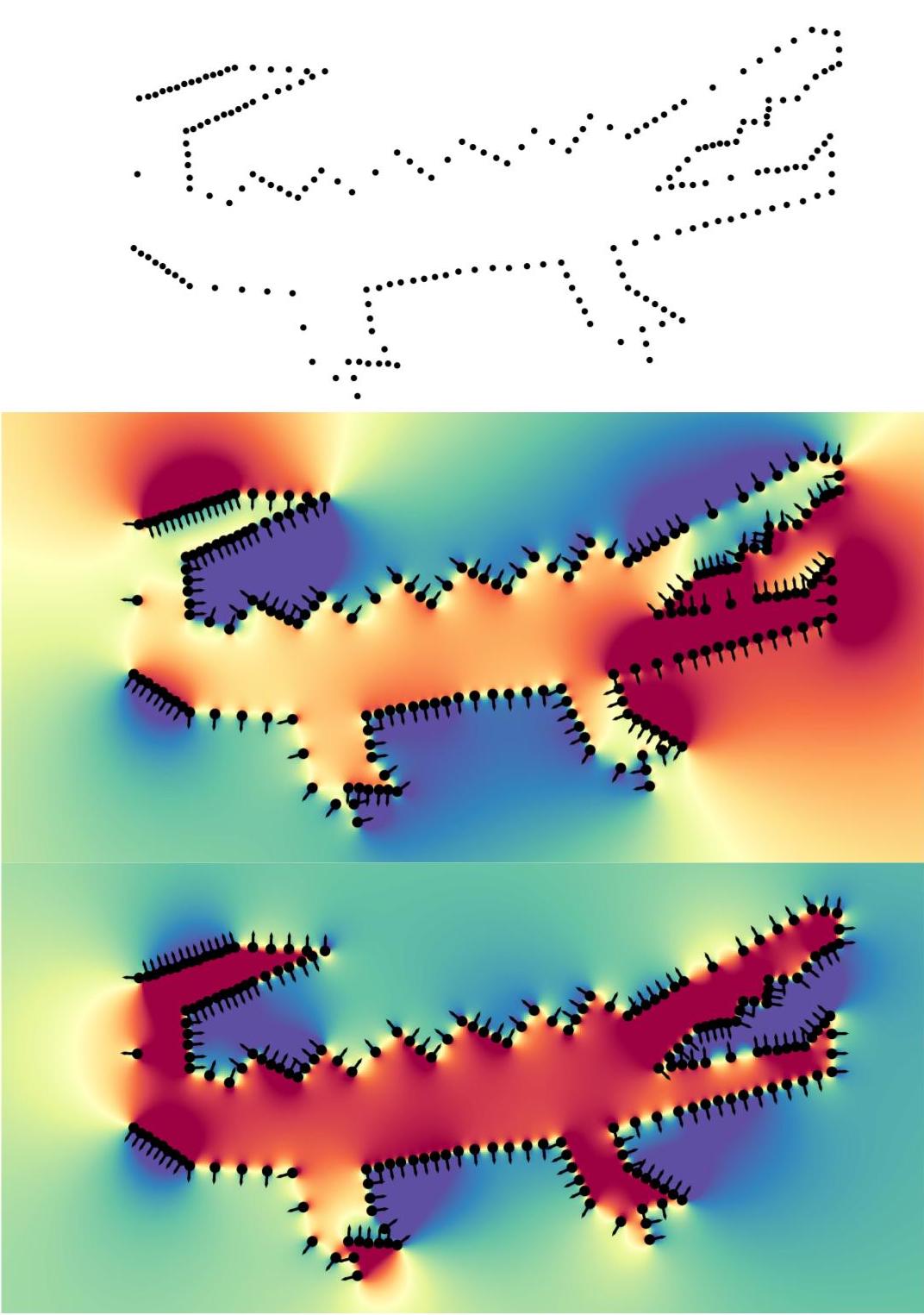
Figure 14. Top: input, middle: [König and Gumhold, 2009], bottom: ours.

5. Experiments

We evaluate our technique on a series of qualitative and quantitative experiments on a range of different point clouds from a variety of sources. First, we explain how our method can be used for orientation interpolation in Section 5.1. Then, in Section 5.2, we compare to existing methods on different point cloud resolutions and neural generated point clouds, from scanning devices, and provide runtime evaluations.

The training dataset contains 60 watertight meshes, where some are manufactured shapes (royalty free meshes collected from [Zhou and Jacobson, 2016],  [Wang et al., 2012]), and others are non-rigid shapes from [Romero et al., 2017]. This results in 1410 training patches, where each patch is augmented many times with noise and different reference points for the normal direction supervision.

5.1. Orientation Interpolation

There are a couple of scenarios where it may be desirable to use a given orientation of a set of points to decide the orientation of new points. In these scenarios, it will be convenient to build the electric field $\vec{E}$ from the given orientations, instead of propagating from scratch. For example, in the case of point upsampling we can interpolate the newly synthesized points using the input normal orientations (see Figure 15). Specifically, we calculate the field generated by the given oriented point normals in the direction of Equation (2), and then orient the remaining points.

\begin{overpic}[width=433.62pt]{figures/013_orientation_interpolation-1.png} \put(9.0,-3.7){{\color[rgb]{0,0,0}Input}} \put(35.0,-3.7){{\color[rgb]{0,0,0}EC-Net}} \put(59.0,-3.7){{\color[rgb]{0,0,0}Input}} \put(79.0,-3.7){{\color[rgb]{0,0,0}Self-sample}} \end{overpic}

Figure 15. The input point cloud contains normals (visualized using shading), which are consolidated using [Yu et al., 2018a] and [Metzer et al., 2020]. Given the input normals, we use our orientation interpolation to predict the orientation of the newly synthesized points, resulting in accurate normal preservation. Then we enable diffusion to use the estimated electric field to re-correct the given input normals, which fixes errors (highlighted insets). Note that we (correctly) see the red (interior) since the front facing part of the surface is missing from the input point cloud scan.

In the case of very large point clouds (more than $500,000$ points), we speed-up computation time by performing orientation on a sub-sampled version of the point cloud patches. Then we can orient the remaining points by calculating the field of the subset and using that to orient the remaining point normals. We use this scenario in a comparison to Schertler et al. [2017] in Section 5.2, which focuses on orienting large point clouds. Our proposed speedup results in improved normal orientation accuracy and a significant computational speed up.

5.2. Comparisons

Low resolution point clouds

In order to compare to the variational technique VIPSS [Huang et al., 2019], which is limited to a couple thousand point clouds, we used a point cloud from their dataset containing 500 points and ran PSR [Kazhdan et al., 2006] on the result of three different normal orientation methods in Figure 16. Since PCP-Net [Guerrero et al., 2018] predicts global orientation from local patches, it struggles on concave parts, resulting in undesirable reconstruction results. Our reconstruction result is on-par with VIPSS. However, note that their method does not scale well beyond what is presented.

\begin{overpic}[width=346.89731pt]{figures/011_vipss_kitten.png} \put(8.0,-3.7){{\color[rgb]{0,0,0}PCP-Net}} \put(45.0,-3.7){{\color[rgb]{0,0,0}VIPSS}} \put(80.0,-3.7){{\color[rgb]{0,0,0}Ours}} \end{overpic}

Figure 16. Surface reconstruction from a small amount of unoriented points (500) used with Poisson reconstruction [Kazhdan, 2005]. VIPSS [Huang et al., 2019] is a recent variational approach which produces favorable results for small point clouds, but does not scale to point clouds above a couple thousand. PCP-Net struggles on shapes with concave parts.

Large scanned point clouds

We demonstrate the ability of our technique to handle very large point clouds obtained from scanners [Laric, 2012], both in terms of accuracy and run-time. We ran a comparison on a point cloud with over one million points (Figure 6) and compared to QPBO [Schertler et al., 2017] with Xie et al. [2003] criterion, and to Hoppe et al. [1992] (using CGAL [The CGAL Project, 2020] implementation). Our normal orientation (and corresponding reconstruction) obtains the best accuracy and takes 13 minutes to compute. The method of Hoppe et al. [1992] is fastest to compute (2 minutes), but contains undesirable errors in the mouth region, resulting in poor reconstruction results. QPBO took the longest to compute (90 minutes), and contains the most error.

In Figure 17 we show another example of normal orientation for over 700k points with the corresponding surface reconstruction results.

\begin{overpic}[width=390.25534pt]{figures/012_lion.png} \put(12.0,-3.7){{\color[rgb]{0,0,0}QPBO}} \put(40.0,-3.7){{\color[rgb]{0,0,0}Hoppe}} \put(69.0,-3.7){{\color[rgb]{0,0,0}Ours}} \end{overpic}

Figure 17. Normal orientation estimation and corresponding reconstruction results on a large (700k) scanned point cloud.

For more results on large point clouds from scanned data, including one with 10 million points, see the supplementary material. A point cloud with 10 million points takes 40 minutes to calculate normal orientation with our method (for reference, writing this point cloud to disk takes 10 minutes).

Neural-generated point clouds

We evaluate our method on point clouds generated using several different neural networks. Since there is no ground-truth for these examples, we visualize the estimated normal direction by shading each point with respect to the camera view (where angles larger than $100^{\circ}$ are highlighted in red).

In the case of neural point cloud consolidation, we generate consolidated clouds using EC-Net [Yu et al., 2018a] and Metzer et al. [2020], and visualize the results of our normal orientation compared against two other techniques in Figure 19 and and 18, respectively. Since these techniques upsample / generate new points alongside input points which contain oriented normals, we provide an additional visualization which uses our normal orientation interpolation (shown in Figure 15) as a reference to compute the angle error colors. Our visualization is useful in the case of the consolidated output of EC-Net, which has an input with an interior surface sheet which has an ambiguous orientation (see Figure 15).

\begin{overpic}[width=390.25534pt]{figures/009_self_sample_alien.jpg} \put(8.0,-2.0){{\color[rgb]{0,0,0}QPBO}} \put(33.0,-2.0){{\color[rgb]{0,0,0}Hoppe}} \put(58.0,-2.0){{\color[rgb]{0,0,0}Ours}} \end{overpic}

Figure 18. Consistent normal orientation results on a consolidated point cloud generated from Metzer et al. [2020]. The top row contains the reconstruction results for each of the methods, and the middle and bottom rows are different visualizations (since there is no ground-truth) of the estimated normal orientations. Middle row uses a normal to viewpoint shading, and the bottom row uses a proxy to ground-truth using our interpolation propagation (shown in Figure 15). The result of our method is by orientating the point cloud from scratch (without using the input normals as a reference).

\begin{overpic}[width=433.62pt]{figures/008_screw_results.jpg} \put(8.0,-4.0){{\color[rgb]{0,0,0}Hoppe}} \put(45.0,-4.0){{\color[rgb]{0,0,0}QPBO}} \put(80.0,-4.0){{\color[rgb]{0,0,0}Ours}} \end{overpic}

Figure 19. Consistent normal orientation results on a scanned point cloud consolidated using EC-Net [Yu et al., 2018a]. Since there is no ground-truth, we generated a proxy to ground-truth using the input point cloud normals and our interpolation propagation (top), as well as with thresholded viewpoint shading (bottom). The result of our method is by orientating the point cloud from scratch (without using the input normals as a reference).

We also generate two different point clouds using a point completion network [Yuan et al., 2018], which synthesizes point clouds without any input/given normal information. We compare the orientation results in Figure 20. Note that this example is especially challenging as it also contains points inside the shape (i.e, interior points). More orientation results on point clouds generated from scratch using neural networks [Cai et al., 2020] can be found in the supplementary material.

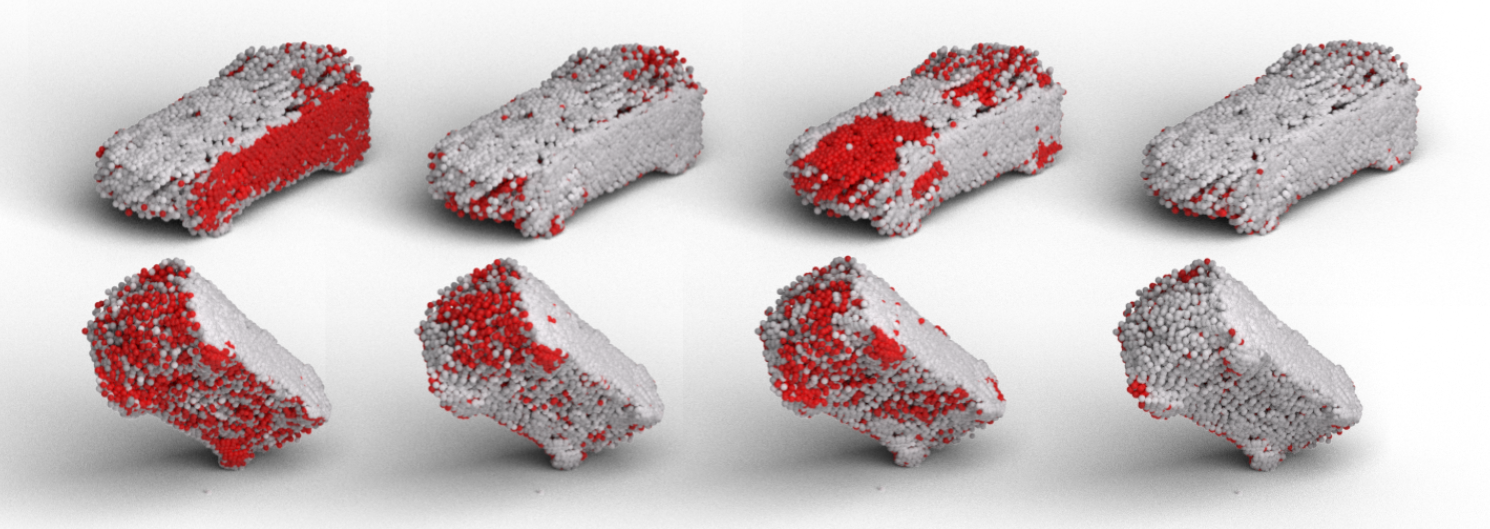
\begin{overpic}[width=433.62pt]{figures/pcn/75_3/pcn_75_3.png} \put(12.0,0.0){{\color[rgb]{0,0,0}Hoppe}} \put(36.0,0.0){{\color[rgb]{0,0,0}König}} \put(59.0,0.0){{\color[rgb]{0,0,0}QPBO}} \put(85.0,0.0){{\color[rgb]{0,0,0}Ours}} \end{overpic}

Figure 20. Normal orientation results on two different point clouds generated using a shape completion network [Yuan et al., 2018] (different viewpoint in top and bottom row). Since there is no ground-truth normal orientation, we visualize the estimated normal direction by shading each point. Note that there are also interior points inside the shape, making normal orientation particularly challenging and even ambiguous.

Quantitative comparison and ablation

For quantitative evaluations, we generated a collection of non-uniformly sampled and noisy point clouds which are used as input for normal orientation. This evaluation data contain two groups: (i) hands from MANO [Romero et al., 2017] and aliens from COSEG [Sidi et al., 2011] with 5-15K points each, and (ii) scanned cloud data from [Laric, 2012] with 700k+ points each. We calculated the percentage of correctly oriented normals in Table 1. Several visual results are shown in Figures 5, 6, and 17, as well as in the supplementary material.

We also ran an ablation where we do not use the network, in order to highlight the effect of the neural network and presented the results in the same table (denoted as No Net) as well as in Figure 9. Instead of using the neural network to estimate coherent normal directions per patch, we calculated the normal orientation of each patch using Jets [Cazals and Pouget, 2005] directed towards the center of mass of each patch. Then we employ dipole propagation (without any network estimated probabilities), and then diffusion. Indeed, the performance drops significantly without a network. In addition, we ran another experiment on a point-based (instead of patch-based) variant of the no-network ablation which results in another performance drop, and does not scale well (computationally) to large point clouds (see supplementary material).

Table 1. Quantitative comparison. Large point clouds (700k+) in the middle two rows. The run-times for the medium sized point clouds are: $30\pm 2$ [seconds] for our method, 3, 4 [seconds] for Hoppe and König respectively, $2$ minutes for QPBO, and $5$ minutes for PCP.

Shape	Hoppe	König	PCP	QPBO	No Net	Ours
09-41r	90	99	86	99	74	99
50-50l	92	97	90	95	74	95
09-39l	89	95	81	96	75	95
17-42l	93	93	89	99	63	99
37-31r	90	99	96	100	75	100
43-16l	90	98	88	99	75	99
a-198	78	90	95	98	62	97
a-160	90	91	97	98	78	98
a-152	88	95	97	100	99	99
a-188	82	86	95	96	90	97
a-158	91	91	96	98	77	98
a-128	55	69	92	90	60	93
a-121	64	84	92	96	68	94
lion	84	78	–	53	–	89
dragon	52	50	–	60	–	95
avg	81	87	91	91	74	96
std	13.23	12.9	4.76	14.14	10.4	2.91

6. Discussion and Future Work

In this paper, we presented a novel technique for estimating a consistent normal orientation for point clouds using a data-driven neural network and dipole-propagation. Our experiments demonstrate that the proposed technique is an effective tool for point cloud normal orientation.

A notable and unique feature of the orientation problem is that it is a global problem, which unlike many other consolidation problems, such as denoising or normal estimation, necessarily requires a global solution. This suggests that a careful design is needed for the solution to scale to a large number of points. Our solution tackles this using a bottom-up approach, where at the bottom a network solves the local high-frequency problems, and the global problem is tackled by dissipating the electric field incrementally by propagation.

Locally, at the patch level, our solution is based on a unique majority-based training technique, which works surprisingly well. Training a network to predict and understand the majority is hard, and it indeed limits the size of the local patch and its variation. On the one hand, taking the patch size to the limit would allow an end-to-end solution, but would be challenging to train and nearly impossible to generalize to unseen shapes. On the other hand, overly small patches would reduce the problem to an unstable point-level solution. We believe that majority-based problems solved by networks have more intriguing potential for additional geometric problems.

An important property of dipole propagation is that it leads to a non-local traversal. This is notable in Figure 1 (and in the accompanying video), where the patch traversal has leaps, and non-local steps. This implicitly suggests that the solution leads to a global one. However, as we showed, there are still a small amount of sporadic erroneous orientations. We recognize that some errors are unavoidable due to significant noise, yet, in the future we plan to investigate randomization techniques. For example, we can train a number of ensemble networks, where each is trained slightly differently with varying patch sizes, and during inference we propagate the results and consult them and vote. Another direction, is to remove outlier points with unstable orientation. This can possibly be achieved by coupling the orientation problem with an implicit function for reconstruction, and normal estimation. Indeed, we believe that the orientation problem is tightly-coupled with surface reconstruction, which is another interesting avenue for future work.

We are encouraged by the global nature of the dipole field, and in the future we want to consider other harmonic functions with minimum oscillations coupled with the power of neural networks. We believe that this combination can be applied to other geometric problems, to quickly infer a solution associated with an informative confidence score.

\begin{overpic}[width=433.62pt]{figures/015_limitation.jpg} \put(18.0,-3.7){{\color[rgb]{0,0,0}Input}} \put(65.0,-3.7){{\color[rgb]{0,0,0}Output}} \end{overpic}

Figure 21. Our technique is designed to handle point clouds which represent the exterior of an object. When using our technique to orient a general polygon soup from shapes in Modelnet, our approach works on simple models (top) with some interior protrusion from the legs, but fails to handle the challenging soup (bottom) with complex interior surfaces.

Our method is designed to orient point clouds which represent the exterior of an object. Although it may be natural to use the same approach to orient general polygon soups, for example, to obtain consistent facet normals for models in Modelnet [Wu et al., 2015]. While our approach works on simple models, it fails to handle challenging soups with multiple internal surfaces (see Figure 21). Extending our approach to this case is an interesting avenue for future work.

We believe that combining dipole proportion techniques with visibility approaches has great potential in solving notoriously challenging problems in geometry processing.

- [1]
- Achlioptas et al. [2018] Panos Achlioptas, Olga Diamanti, Ioannis Mitliagkas, and Leonidas Guibas. 2018. Learning representations and generative models for 3d point clouds. In International conference on machine learning. PMLR, 40–49.
- Barill et al. [2018] Gavin Barill, Neil Dickson, Ryan Schmidt, David I.W. Levin, and Alec Jacobson. 2018. Fast Winding Numbers for Soups and Clouds. ACM Transactions on Graphics (2018).
- Cai et al. [2020] Ruojin Cai, Guandao Yang, Hadar Averbuch-Elor, Zekun Hao, Serge Belongie, Noah Snavely, and Bharath Hariharan. 2020. Learning Gradient Fields for Shape Generation. In Proceedings of the European Conference on Computer Vision (ECCV).
- Cazals and Pouget [2005] Frédéric Cazals and Marc Pouget. 2005. Estimating differential quantities using polynomial fitting of osculating jets. Computer Aided Geometric Design 22, 2 (2005), 121–146.
- Chen et al. [2010] Yi-Ling Chen, Bing-Yu Chen, Shang-Hong Lai, and Tomoyuki Nishita. 2010. Binary orientation trees for volume and surface reconstruction from unoriented point clouds. In Computer Graphics Forum, Vol. 29. Wiley Online Library, 2011–2019.
- Fan et al. [2017] Haoqiang Fan, Hao Su, and Leonidas J Guibas. 2017. A point set generation network for 3d object reconstruction from a single image. In Proceedings of the IEEE conference on computer vision and pattern recognition. 605–613.
- Folland [1995] Gerald B Folland. 1995. Introduction to partial differential equations. Vol. 102. Princeton university press.
- Groueix et al. [2018] Thibault Groueix, Matthew Fisher, Vladimir G Kim, Bryan C Russell, and Mathieu Aubry. 2018. A papier-mâché approach to learning 3d surface generation. In Proceedings of the IEEE conference on computer vision and pattern recognition. 216–224.
- Guennebaud and Gross [2007] Gaël Guennebaud and Markus Gross. 2007. Algebraic point set surfaces. In ACM SIGGRAPH 2007 papers. 23–es.
- Guerrero et al. [2018] Paul Guerrero, Yanir Kleiman, Maks Ovsjanikov, and Niloy J Mitra. 2018. Pcpnet learning local shape properties from raw point clouds. In Computer Graphics Forum, Vol. 37. Wiley Online Library, 75–85.
- Gurumurthy and Agrawal [2019] Swaminathan Gurumurthy and Shubham Agrawal. 2019. High fidelity semantic shape completion for point clouds using latent optimization. In 2019 IEEE Winter Conference on Applications of Computer Vision (WACV). IEEE, 1099–1108.
- Hanocka et al. [2019] Rana Hanocka, Amir Hertz, Noa Fish, Raja Giryes, Shachar Fleishman, and Daniel Cohen-Or. 2019. MeshCNN: A Network with an Edge. ACM Trans. Graph. 38, 4, Article 90 (July 2019), 12 pages. https://doi.org/10.1145/3306346.3322959
- Hanocka et al. [2020] Rana Hanocka, Gal Metzer, Raja Giryes, and Daniel Cohen-Or. 2020. Point2Mesh: A Self-Prior for Deformable Meshes. ACM Trans. Graph. 39, 4, Article 126 (July 2020), 12 pages. https://doi.org/10.1145/3386569.3392415
- Hermosilla et al. [2019] Pedro Hermosilla, Tobias Ritschel, and Timo Ropinski. 2019. Total Denoising: Unsupervised learning of 3D point cloud cleaning. In Proceedings of the IEEE International Conference on Computer Vision. 52–60.
- Hertz et al. [2020] Amir Hertz, Rana Hanocka, Raja Giryes, and Daniel Cohen-Or. 2020. PointGMM: a Neural GMM Network for Point Clouds. In Proceedings of the IEEE/CVF Conference on Computer Vision and Pattern Recognition. 12054–12063.
- Hoppe et al. [1992] Hugues Hoppe, Tony DeRose, Tom Duchamp, John McDonald, and Werner Stuetzle. 1992. Surface reconstruction from unorganized points. In Proceedings of the 19th annual conference on Computer graphics and interactive techniques. 71–78.
- Huang et al. [2020] Chao Huang, Ruihui Li, Xianzhi Li, and Chi-Wing Fu. 2020. Non-Local Part-Aware Point Cloud Denoising. arXiv preprint arXiv:2003.06631 (2020).
- Huang et al. [2009] Hui Huang, Dan Li, Hao Zhang, Uri Ascher, and Daniel Cohen-Or. 2009. Consolidation of unorganized point clouds for surface reconstruction. ACM transactions on graphics (TOG) 28, 5 (2009), 1–7.
- Huang et al. [2019] Zhiyang Huang, Nathan Carr, and Tao Ju. 2019. Variational implicit point set surfaces. ACM Transactions on Graphics (TOG) 38, 4 (2019), 1–13.
- Jakob et al. [2019] Johannes Jakob, Christoph Buchenau, and Michael Guthe. 2019. Parallel globally consistent normal orientation of raw unorganized point clouds. In Computer Graphics Forum, Vol. 38. Wiley Online Library, 163–173.
- Jiang et al. [2018] Li Jiang, Shaoshuai Shi, Xiaojuan Qi, and Jiaya Jia. 2018. Gal: Geometric adversarial loss for single-view 3d-object reconstruction. In Proceedings of the European Conference on Computer Vision (ECCV). 802–816.
- Katz et al. [2007] Sagi Katz, Ayellet Tal, and Ronen Basri. 2007. Direct visibility of point sets. In ACM SIGGRAPH 2007 papers. 24–es.
- Kazhdan [2005] Michael Kazhdan. 2005. Reconstruction of solid models from oriented point sets. In Proceedings of the third Eurographics symposium on Geometry processing. 73–es.
- Kazhdan et al. [2006] Michael Kazhdan, Matthew Bolitho, and Hugues Hoppe. 2006. Poisson surface reconstruction. In Proceedings of the fourth Eurographics symposium on Geometry processing, Vol. 7.
- Kazhdan and Hoppe [2013] Michael Kazhdan and Hugues Hoppe. 2013. Screened poisson surface reconstruction. ACM Transactions on Graphics (ToG) 32, 3 (2013), 1–13.
- König and Gumhold [2009] S. König and S. Gumhold. 2009. Consistent Propagation of Normal Orientations in Point Clouds. In VMV.
- Lang et al. [2020] Itai Lang, Uriel Kotlicki, and Shai Avidan. 2020. Geometric Adversarial Attacks and Defenses on 3D Point Clouds. arXiv preprint arXiv:2012.05657 (2020).
- Laric [2012] Oliver Laric. 2012. Three D Scans. http://threedscans.com/info/ (2012).
- Levin [2004] David Levin. 2004. Mesh-independent surface interpolation. In Geometric modeling for scientific visualization. Springer, 37–49.
- Li et al. [2018c] Chun-Liang Li, Manzil Zaheer, Yang Zhang, Barnabas Poczos, and Ruslan Salakhutdinov. 2018c. Point cloud gan. arXiv preprint arXiv:1810.05795 (2018).
- Li et al. [2018b] Jiaxin Li, Ben M Chen, and Gim Hee Lee. 2018b. So-net: Self-organizing network for point cloud analysis. In Proceedings of the IEEE conference on computer vision and pattern recognition. 9397–9406.
- Li et al. [2019] Ruihui Li, Xianzhi Li, Chi-Wing Fu, Daniel Cohen-Or, and Pheng-Ann Heng. 2019. Pu-gan: a point cloud upsampling adversarial network. In Proceedings of the IEEE International Conference on Computer Vision. 7203–7212.
- Li et al. [2018a] Yangyan Li, Rui Bu, Mingchao Sun, Wei Wu, Xinhan Di, and Baoquan Chen. 2018a. Pointcnn: Convolution on x-transformed points. In Advances in neural information processing systems. 820–830.
- Liu et al. [2020] Minghua Liu, Lu Sheng, Sheng Yang, Jing Shao, and Shi-Min Hu. 2020. Morphing and sampling network for dense point cloud completion. In Proceedings of the AAAI Conference on Artificial Intelligence, Vol. 34. 11596–11603.
- Liu et al. [2019] Xinhai Liu, Zhizhong Han, Xin Wen, Yu-Shen Liu, and Matthias Zwicker. 2019. L2g auto-encoder: Understanding point clouds by local-to-global reconstruction with hierarchical self-attention. In Proceedings of the 27th ACM International Conference on Multimedia. 989–997.
- Luo and Hu [2020] Shitong Luo and Wei Hu. 2020. Differentiable Manifold Reconstruction for Point Cloud Denoising. In Proceedings of the 28th ACM International Conference on Multimedia. 1330–1338.
- Mello et al. [2003] Viní cius Mello, Luiz Velho, and Gabriel Taubin. 2003. Estimating the in/out function of a surface represented by points. In Proceedings of the eighth ACM symposium on Solid modeling and applications. 108–114.
- Metzer et al. [2020] Gal Metzer, Rana Hanocka, Raja Giryes, and Daniel Cohen-Or. 2020. Self-Sampling for Neural Point Cloud Consolidation. arXiv preprint arXiv:2008.06471 (2020).
- Mitra and Nguyen [2003] Niloy J Mitra and An Nguyen. 2003. Estimating surface normals in noisy point cloud data. In Proceedings of the nineteenth annual symposium on Computational geometry. 322–328.
- Mullen et al. [2010] Patrick Mullen, Fernando De Goes, Mathieu Desbrun, David Cohen-Steiner, and Pierre Alliez. 2010. Signing the unsigned: Robust surface reconstruction from raw pointsets. In Computer Graphics Forum, Vol. 29. Wiley Online Library, 1733–1741.
- Park et al. [2019] Jeong Joon Park, Peter Florence, Julian Straub, Richard Newcombe, and Steven Lovegrove. 2019. DeepSDF: Learning Continuous Signed Distance Functions for Shape Representation. In The IEEE Conference on Computer Vision and Pattern Recognition (CVPR).
- Pauly et al. [2003] Mark Pauly, Richard Keiser, Leif P Kobbelt, and Markus Gross. 2003. Shape modeling with point-sampled geometry. ACM Transactions on Graphics (TOG) 22, 3 (2003), 641–650.
- Pistilli et al. [2020] Francesca Pistilli, Giulia Fracastoro, Diego Valsesia, and Enrico Magli. 2020. Learning Graph-Convolutional Representations for Point Cloud Denoising. In European Conference on Computer Vision. Springer, 103–118.
- Qi et al. [2017a] Charles R Qi, Hao Su, Kaichun Mo, and Leonidas J Guibas. 2017a. Pointnet: Deep learning on point sets for 3d classification and segmentation. In Proceedings of the IEEE conference on computer vision and pattern recognition. 652–660.
- Qi et al. [2017b] Charles Ruizhongtai Qi, Li Yi, Hao Su, and Leonidas J Guibas. 2017b. Pointnet++: Deep hierarchical feature learning on point sets in a metric space. Advances in neural information processing systems 30 (2017), 5099–5108.
- Rakotosaona et al. [2020] Marie-Julie Rakotosaona, Vittorio La Barbera, Paul Guerrero, Niloy J Mitra, and Maks Ovsjanikov. 2020. Pointcleannet: Learning to denoise and remove outliers from dense point clouds. In Computer Graphics Forum, Vol. 39. Wiley Online Library, 185–203.
- Romero et al. [2017] Javier Romero, Dimitrios Tzionas, and Michael J. Black. 2017. Embodied Hands: Modeling and Capturing Hands and Bodies Together. ACM Transactions on Graphics, (Proc. SIGGRAPH Asia) 36, 6 (Nov. 2017).
- Sarmad et al. [2019] Muhammad Sarmad, Hyunjoo Jenny Lee, and Young Min Kim. 2019. Rl-gan-net: A reinforcement learning agent controlled gan network for real-time point cloud shape completion. In Proceedings of the IEEE Conference on Computer Vision and Pattern Recognition. 5898–5907.
- Schertler et al. [2017] Nico Schertler, Bogdan Savchynskyy, and Stefan Gumhold. 2017. Towards globally optimal normal orientations for large point clouds. In Computer Graphics Forum, Vol. 36. Wiley Online Library, 197–208.
- Seversky et al. [2011] Lee M Seversky, Matt S Berger, and Lijun Yin. 2011. Harmonic point cloud orientation. Computers & Graphics 35, 3 (2011), 492–499.
- Sidi et al. [2011] Oana Sidi, Oliver van Kaick, Yanir Kleiman, Hao Zhang, and Daniel Cohen-Or. 2011. Unsupervised co-segmentation of a set of shapes via descriptor-space spectral clustering. In Proceedings of the 2011 SIGGRAPH Asia Conference. 1–10.
- Sun et al. [2020] Yongbin Sun, Yue Wang, Ziwei Liu, Joshua Siegel, and Sanjay Sarma. 2020. Pointgrow: Autoregressively learned point cloud generation with self-attention. In The IEEE Winter Conference on Applications of Computer Vision. 61–70.
- Tchapmi et al. [2019] Lyne P Tchapmi, Vineet Kosaraju, Hamid Rezatofighi, Ian Reid, and Silvio Savarese. 2019. Topnet: Structural point cloud decoder. In Proceedings of the IEEE Conference on Computer Vision and Pattern Recognition. 383–392.
- The CGAL Project [2020] The CGAL Project. 2020. CGAL User and Reference Manual (5.2 ed.). CGAL Editorial Board. https://doc.cgal.org/5.2/Manual/packages.html
- Walder et al. [2005] Christian Walder, Olivier Chapelle, and Bernhard Schölkopf. 2005. Implicit surface modelling as an eigenvalue problem. In Proceedings of the 22nd international conference on Machine learning. 936–939.
- Wang et al. [2020] Xiaogang Wang, Marcelo H Ang Jr, and Gim Hee Lee. 2020. Point Cloud Completion by Learning Shape Priors. arXiv preprint arXiv:2008.00394 (2020).
- Wang et al. [2012] Yunhai Wang, Shmulik Asafi, Oliver Van Kaick, Hao Zhang, Daniel Cohen-Or, and Baoquan Chen. 2012. Active co-analysis of a set of shapes. ACM Transactions on Graphics (TOG) 31, 6 (2012), 1–10.
- Wang et al. [2019] Yue Wang, Yongbin Sun, Ziwei Liu, Sanjay E Sarma, Michael M Bronstein, and Justin M Solomon. 2019. Dynamic graph cnn for learning on point clouds. Acm Transactions On Graphics (tog) 38, 5 (2019), 1–12.
- Wen et al. [2020] Xin Wen, Tianyang Li, Zhizhong Han, and Yu-Shen Liu. 2020. Point cloud completion by skip-attention network with hierarchical folding. In Proceedings of the IEEE/CVF Conference on Computer Vision and Pattern Recognition. 1939–1948.
- Williams et al. [2019] Francis Williams, Teseo Schneider, Claudio Silva, Denis Zorin, Joan Bruna, and Daniele Panozzo. 2019. Deep geometric prior for surface reconstruction. In Proceedings of the IEEE Conference on Computer Vision and Pattern Recognition. 10130–10139.
- Wu et al. [2015] Zhirong Wu, Shuran Song, Aditya Khosla, Fisher Yu, Linguang Zhang, Xiaoou Tang, and Jianxiong Xiao. 2015. 3d shapenets: A deep representation for volumetric shapes. In Proceedings of the IEEE conference on computer vision and pattern recognition. 1912–1920.
- Xie et al. [2004] Hui Xie, Kevin T McDonnell, and Hong Qin. 2004. Surface reconstruction of noisy and defective data sets. In IEEE Visualization 2004. IEEE, 259–266.
- Xie et al. [2003] Hui Xie, Jianning Wang, Jing Hua, Hong Qin, and Arie Kaufman. 2003. Piecewise C/sup 1/continuous surface reconstruction of noisy point clouds via local implicit quadric regression. In IEEE Visualization, 2003. VIS 2003. IEEE, 91–98.
- Xu et al. [2018] Minfeng Xu, Shiqing Xin, and Changhe Tu. 2018. Towards globally optimal normal orientations for thin surfaces. Computers & Graphics 75 (2018), 36–43.
- Yang et al. [2019] Guandao Yang, Xun Huang, Zekun Hao, Ming-Yu Liu, Serge Belongie, and Bharath Hariharan. 2019. Pointflow: 3d point cloud generation with continuous normalizing flows. In Proceedings of the IEEE International Conference on Computer Vision. 4541–4550.
- Yang et al. [2018] Yaoqing Yang, Chen Feng, Yiru Shen, and Dong Tian. 2018. Foldingnet: Point cloud auto-encoder via deep grid deformation. In Proceedings of the IEEE Conference on Computer Vision and Pattern Recognition. 206–215.
- Yifan et al. [2019a] Wang Yifan, Felice Serena, Shihao Wu, Cengiz Öztireli, and Olga Sorkine-Hornung. 2019a. Differentiable surface splatting for point-based geometry processing. ACM Transactions on Graphics (TOG) 38, 6 (2019), 1–14.
- Yifan et al. [2019b] Wang Yifan, Shihao Wu, Hui Huang, Daniel Cohen-Or, and Olga Sorkine-Hornung. 2019b. Patch-based progressive 3d point set upsampling. In Proceedings of the IEEE Conference on Computer Vision and Pattern Recognition. 5958–5967.
- Yu et al. [2018a] Lequan Yu, Xianzhi Li, Chi-Wing Fu, Daniel Cohen-Or, and Pheng-Ann Heng. 2018a. Ec-net: an edge-aware point set consolidation network. In Proceedings of the European Conference on Computer Vision (ECCV). 386–402.
- Yu et al. [2018b] Lequan Yu, Xianzhi Li, Chi-Wing Fu, Daniel Cohen-Or, and Pheng-Ann Heng. 2018b. Pu-net: Point cloud upsampling network. In Proceedings of the IEEE Conference on Computer Vision and Pattern Recognition. 2790–2799.
- Yuan et al. [2018] Wentao Yuan, Tejas Khot, David Held, Christoph Mertz, and Martial Hebert. 2018. Pcn: Point completion network. In 2018 International Conference on 3D Vision (3DV). IEEE, 728–737.
- Zhao et al. [2019] Yongheng Zhao, Tolga Birdal, Haowen Deng, and Federico Tombari. 2019. 3D point capsule networks. In Proceedings of the IEEE conference on computer vision and pattern recognition. 1009–1018.
- Zhou and Jacobson [2016] Qingnan Zhou and Alec Jacobson. 2016. Thingi10K: A Dataset of 10,000 3D-Printing Models. arXiv preprint arXiv:1605.04797 (2016).