Chapter
Information analysis in free and confined harmonic oscillator

Abstract

In this chapter we shall discuss the recent progresses of information theoretic tools in the context of free and confined harmonic oscillator (CHO). Confined quantum systems have provided appreciable interest in areas of physics, chemistry, biology, etc., since its inception. A particle under extreme pressure environment unfolds many fascinating, notable physical and chemical changes. The desired effect is achieved by reducing the spatial boundary from infinity to a finite region. Similarly, in the last decade, information measures were investigated extensively in diverse quantum problems, in both free and constrained situations. The most prominent amongst these are: Fisher information ($I$), Shannon entropy ($S$), Rényi entropy ($R$), Tsallis entropy ($T$), Onicescu energy ($E$) and several complexities. Arguably, these are the most effective measures of uncertainty, as they do not make any reference to some specific points of a respective Hilbert space. These have been invoked to explain several physico-chemical properties of a system under investigation. Kullback$–$Leibler divergence or relative entropy describes how a given probability distribution shifts from a reference distribution function. This characterizes a measure of discrimination between two states. In other words, it extracts the change of information in going from one state to another.

The one-dimensional confined harmonic oscillator (1DCHO), defined by $v(x)=\frac{1}{2}(x-d_{m})^{2}+v_{c}$ ($k$ is the force constant, $v_{c}=0,~{}x<x_{c}$ and $v_{c}=\infty,~{}x\geq x_{c}$), can be classified into two forms, (a) symmetrically confined harmonic oscillator (SCHO) (when $d_{m}=0$), (b) asymmetrically confined harmonic oscillator (ACHO) (corresponding to $d_{m}\neq 0$). Further, in latter case, confinement can be accomplished two different ways: (i) by changing the box boundary, keeping box length and $d_{m}$ fixed at zero; (ii) another route is to adjust $d_{m}$ by keeping box length and boundary fixed. SCHO can be treated as an intermediate between a particle-in-a-box (PIB) and a 1DQHO. Though the Schrödinger equation for SCHO can be solved exactly, for ACHO it cannot be. We have employed two different methods for the latter, viz., (i) an imaginary time propagation (ITP), leading to minimization of an expectation value (ii) a variation-induced exact diagonalization procedure that utilizes SCHO eigenfunctions as basis. It is found that, at very low $x_{c}$ region, $I,~{}S,~{}R,~{}T,~{}E$ remain invariant with change confinement length, $x_{c}$. At moderate $x_{c}$ region $S_{x},~{}R_{x},~{}T_{x}$ progress and $I_{x},~{}E_{x}$ decrease with rise in $x_{c}$. Additionally, special attention has been paid to study relative information in SCHO and ACHO.

Analogously, a 3DCHO (radically confined within an impenetrable spherical well) can act as a bridge between particle in a spherical box (PISB) and isotropic 3DQHO. The time-independent Schrödinger equation for D-dimensional harmonic oscillator in both free and confined condition can be solved exactly, within a Dirichlet boundary condition. Here a detailed exploration of information measures has been carried out in $r$ and $p$ spaces, for a 3DCHO. Some exact analytical expressions for these quantities have also been presented, wherever possible. Besides we also consider some recent works on relative information and several complexity measures in composite $r$ and $p$ spaces. Also discussion is made of a recently proposed virial theorem in the context of confinement. In essence, this chapter provides a detailed in-depth investigation about the information theoretical analysis in 1DCHO and 3DCHO, as done in our laboratory.

PACS: 03.65-w, 03.65Ca, 03.65Ta, 03.65.Ge, 03.67-a.

Keywords: Rényi entropy, Shannon entropy, Fisher information, Onicescu energy, Complexities, Confined isotropic harmonic oscillator, Particle in a symmetric box.

1. Introduction

“A quantum particle inside an infinite impenetrable box” usually constitutes the first model problem taught in quantum mechanics curriculum. Later, the attention shifts towards the study of “free” systems in some characteristic potential, such as a harmonic oscillator or a H atom in a Coulombic potential, which typify a quantum mechanical problem in a whole region of space. This is itself a recognition of the importance of sub-region $\Omega$ of the space, which in this particular scenario is achieved by modeling the boundary condition. Such a situation arises when one tries to explore systems in highly inhomogeneous media or in intense external field. The limit, when the box becomes very small, approaching quantum size is generally termed as “quantum confinement”. In this microscopic domain, confinement occurs on a scale comparable to atomic size (object and cavity sizes are commensurate), which is in sharp contrast to the ordinary confinement, where the cavity size is usually much larger than the atom. Classic examples of such macroscopic-size boxes are found in celebrated physics problems like kinetic theory of gas, black-body radiation, atom in a microwave enclosure, etc.

The first seminal work in this direction is due to a pioneering article [1] published in the fourth decade of twentieth century, where the effect of pressure on static polarizability of a H atom enclosed inside a spherical impenetrable hard enclosure was studied. It was realized that certain properties (such as energy/eigenvalue, orbital/eigenfunction, electron localization, shell-filling, polarizability, photonic ionization/absorption, etc., to name a few) of an atom could be significantly altered by “squeezing” or ”shrinking” it by placing inside a hard sphere, which acts as an idealized classical piston. Depending on the geometrical form and dimension of cavity, such characteristic features of a caged-in atom exhibits numerous deviations from corresponding free atom. Apparently there was some paucity in their immediate applications, but in the last few decades, these models have found wide-spread applications in various branches in physics and chemistry. Lately there has been a plethora of activities in harnessing their potential in various physico-chemical situations as evidenced by an almost exponential growth in the number of articles published in journals, and this continues to grow day by day. Excellent elegant reviews have been made available on the subject; we mention here a very selected set [2, 3, 4, 5, 6].

With the advancement of modern technology, confined quantum systems has emerged as an extremely important contemporary research area, from both theoretical and experimental perspectives. The discovery and development of modern experimental techniques have provided the desired impetus about these boxed-in systems. Constrained atoms, molecules inside various cavities has shed light on their electronic structure, chemical reactivity under high pressure. Apart from that, their relevance has been advocated in numerous other instances, such as impurity in semiconductor/nanostructure, atoms trapped in zeolite sieves or fullerene cage, solutes under solvent environment, artificial atom like quantum dot, quantum wire, quantum well, etc. Recently endohedral metallofullerene clusters where atoms/molecules are typically encapsulated in carbon (or fullerene-like inorganic and hybrid) cages of varying size, shape has found promising applications [7, 8, 9] in engineering. The subtle interaction between host cage and inserted guest molecule is manifested in their marked structural, energetic and spectroscopic properties of endocluster, in comparison to the isolated guest molecule or empty cavity.

The confined harmonic oscillator (CHO) remains one of the oldest, heavily studied model of quantum confinement. In this case the quadratic potential acts through only a finite distance corresponding to the length of box; beyond this an infinite repulsive potential exists. This has been used in the context of various complicated physical situations ever since its inception. Some noteworthy applications include energy generation in dense stars from proton-deuteron transformation [10], mass-radius relation in white dwarf theory [11], rate of escape of a star from a galaxy or globular cumulus [12], electric and magnetic properties of metals including small system of electrons within a cylinder [13, 14], vibronic spectra of point defects, impurities and luminescence in solids [15], specific heats of metal under high pressure, effect of high pressure on properties of materials, etc.

Since the forty’s decade, a vast amount of theoretical methods have been reported for accurate solution of a 1DCHO, placed inside a hard impenetrable symmetric box. The usual boundary condition of wave function vanishing at infinity of unenclosed or free harmonic oscillator (QHO) is replaced by the requirement that it vanishes at the walls of enclosure. Eigenfunctions in such systems could then be written in terms of Kummer’s function [10, 11], whereas the zeros of confluent hypergeometric function provided energy eigenvalues. Further, the authors employed various approaches to expand the latter in order to find an analytical expression in terms of box size. They found the correct qualitative behavior, i.e., energy levels of a 1DCHO increases rapidly as box length diminishes. An asymptotic expression [16] for energy valid in the region of small length of box was derived. An attempt [17] was made to locate the zeros of hypergeometric function numerically, albeit with limited success. It was further established that while in a QHO (wave function vanishing at $\infty$), transitions can occur only between two adjacent levels, in a bounded oscillator, there occurs a non-zero transition probability between any two states of different parity. Simple analytical expressions [18] of energy in certain special cases were put forth. The effect of finite boundary on energy levels has also been pursued graphically and from some series expansion [19]. Later, within a semi-classical Wentzel-Kramers-Brillouin (WKB)-type approximation [20], it was pointed out that eigenvalues of the constrained problem reduce to respective unenclosed oscillators, provided the classical turning points remain inside the potential enclosure and not near the walls. Moreover, when the separation of turning points remains large in comparison to the box size, they become plane-wave box eigenvalues. Subsequently, a series analytical solution [21] was proposed for eigenvalues by keeping the center of oscillation at the center of potential enclosure. Eigenvalues were also computed by a numerical procedure as the roots of a polynomial [22]. It was observed that when the box length remains below a certain critical value (corresponding to the effective oscillation length for an unconfined oscillator of lowest energy), the individual energies dramatically increase from uncaged values. Closed-form energy expressions valid for boxes of any size were derived by constructing Padé approximants [23] as interpolation between the perturbative and asymptotic solutions. Methods such as diagonal hyper-virial [24, 25] as well as hyper-virial perturbation theory [26] were also employed for such enclosed systems for a variety of boundary conditions. A Rayleigh-Ritz variation method utilizing the trigonometric basis functions was suggested in [27]. A numerical scheme [28], based on a set of theorems that guarantee that the solution of SE corresponding to a bounded system strongly converges in the norm of Hilbert space $L_{2}(-\infty,\infty)$ to exact solution of respective unbounded problem. Spatially confined 1DQHO was treated by (WKB) along with modified airy function method [29], as well as super-symmetric WKB approach [30]. Highly accurate eigenvalues were published in [31] by numerically finding zeros of hypergeometric functions. Accurate eigenvalues were computed by power-series method [32], perturbation theory [33], ITP method [34] in conjunction with the minimization of an energy expectation value; in the former also the Einstein coefficients were considered. Very recently, this problem has been revisited by diagonalizing the Hamiltonian using a PIB basis [35]. However, all the above referenced works relate to the so-called symmetric confinement; asymmetric confinement studies are relatively less. For example, in an asymmetric CHO (ACHO), the energy spectrum have been reported by means of perturbation theory [36], power-series method [32] and ITP [34] method. Other properties such dipole moment [36] as well as Einstein coefficients [36, 32] were also considered.

In parallel to the 1DCHO problem, much attention was also paid on 2D, 3D and $N$-dimensional counterparts, albeit with less vigour. A number of interesting unique phenomena occur in higher dimensions, especially in connection to simultaneous, incidental and inter-dimensional degeneracy, which are elaborated later in due course of time. In one of the earliest attempts, bounded multi-dimensional isotropic harmonic oscillators, including a 3DCHO were investigated using a hyper-virial treatment [37]. Energy eigenvalues of 2DCHO and 3DCHO in circular and spherical boxes respectively were reported through Rayleigh-Schrödinger perturbation expansion, considering the free PIB as corresponding unperturbed systems, as well as Padé approximant solution [38]. A 3DCHO within an impenetrable spherical cavity was approached by a direct variational method [39], where the trial wave function was assumed as product of the “free” solution of corresponding SE and a simple function obeying the respective boundary condition. For the 3DCHO, super-symmetric semi-classical approach [40] has been advocated. The radial SE corresponding to the 2DCHO and 3DCHO was solved quite efficiently by means of a variational procedure, whereby the wave function was expanded into a Fourier-Bessel series [41, 42], with matrix elements involving Bessel functions, that could be evaluated analytically. First detailed and systematic calculation of energies, eigenfunctions and spatial expectation values in isotropic 3DCHO was undertaken in [43], employing a variational strategy. Like the 1DCHO case, a WKB approach was also put forth in 3DCHO by the same author [44], where the centrifugal term is expanded perturbatively (in powers of $\hbar$), partitioning in two parts, viz., the usual centrifugal potential governed by classical laws and a quantum correction. A recipe was also provided for 3DCHO within the super-symmetric quantum mechanics [45] in association with variational principle, as well as a generalized pseudo-spectral (GPS) method [46, 47]. Eigenspectra of 2DCHO [48] and 3DCHO [49] were investigated analytically in terms of annihilation and creation operators. A combination of semi-classical WKB method and a proper quantization rule [50] has also been suggested for the spherically confined harmonic oscillator. Some reports have also been made on higher dimensional CHO, although in much lesser intensity. Reasonably [51] and very accurate [52] eigenvalues have been reported for $D$-dimensional CHO from numerical calculations that find the roots of confluent hypergeometric functions satisfying the necessary degeneracy conditions. High-precision energies were presented [31] by exploiting certain special properties of hypergeometric functions within MAPLE computer algebra system.

In the last few decades, quantum information theory has emerged as a subject of topical interest. This concept has been exploited to understand various phenomena in physics and chemistry, with potential applications in broad topics like thermodynamics [53, 54, 55], quantum mechanics [53, 54, 55], spectroscopy etc. Lately, it has been extensively used to understand quantum entanglement and quantum steering problems [53, 54, 55]. The information theoretic measures like Shannon entropy ($S$) [56, 57], Rényi entropy ($R^{\alpha}$) [58], Fisher information ($I$), Onicescu energy ($E$) and complexities ($C$) are invoked to get knowledge about diffusion of atomic orbitals, spread of electron density, periodic properties, correlation energy and so forth. Perhaps, these are the most effective measures of uncertainty [56, 58, 59, 60], as they do not make any reference to some specific points of the respective Hilbert space. In principle, they can have any real value. However, $(-)$ve value in $R$ and $S$ indicates extreme localization, whereas, $E$ is always ($+$)ve. Likewise, changing the numerical values of $R^{\alpha},~{}S$ from $(-)$ve to ($+$)ve only interprets enhancement of de-localization. Another related concept is complexity. A system has finite complexity when it is either in a state with less than some maximal order or not at a state of equilibrium. In a nutshell, it becomes zero at two limiting cases, viz., when a system is (i) completely ordered (maximum distance from equilibrium) or (ii) at equilibrium (maximum disorder). Complexity has its contemporary interest in chaotic systems, spatial patterns, language, multi-electronic systems, molecular or DNA analysis, social science, astrophysics and cosmology etc.

In this chapter, we summarize the recent progress that has taken place in the information theoretical analysis in case of a quantum harmonic oscillator (QHO) contained in inside a hard, impenetrable cage. To this end, a thorough investigation is made for energy spectra and a host of information quantities, like $S,R,I,E,C$, in 1DCHO (symmetric and asymmetric) as well as a radially confined QHO. In the 1D case, we introduce two accurate methods for solution of relevant eigenvalue equations in presence of the Dirichlet boundary conditions, namely (i) ITP and (ii) variation-induced exact diagonalization–both developed in our laboratory. They provide accurate eigenvalues and eigenfunctions, which are used throughout. In the 3D counterpart, we employ the very accurate GPS method. One important conclusion is that, a 1DCHO behaves as an intermediate between a PIB and an 1DQHO. Detailed results are compiled in tabular and graphical form for the afore-mentioned information-related quantities, always indicating the transition from bounded to free system. Additionally we also offer a brief account of the relative information studies that has been studied by us. Finally, we examine the validity and feasibility of a recently proposed virial theorem in the context of such confined systems, which will consolidate the former’s success further. Available literature results have been consulted as and when possible. A few concluding remarks are made at the end.

2. Theoretical Aspects

This section is devoted to the theoretical methods that have been employed for calculation of relevant eigenvalues and eigenfunctions for the spatially confined CHO; both in 1D and 3D. Then we proceed for a discussion on the evaluation of momentum ($p$)-space wave functions from that in position space, as well as for the computation of information-related quantities.

2.1. Position-space wave function

In 1DCHO problem can be categorized into two distinct forms, viz., (i) in the SCHO case, potential minimum is at the origin ($x=0$), leading to a symmetric confinement ($R$ is length of box), ($v_{c}(x)$ is the confinement potential), and (ii) ACHO, where the potential minimum is beyond the origin, as exemplified here through the following relations,

$$-\frac{1}{2}\frac{d^{2}\psi}{dx^{2}}+\frac{1}{2}(x-d)^{2}\psi+V(x)\psi=E\psi,$$

where $V(x)=+\infty$, for $|x|\geq R$ and $V(x)=0$, when $|x|<R$. It represents an infinite square well of width $2R$ with $d$ signifying position of minimum in the potential. The SCHO potential can be solved exactly, whereas in latter case one needs an appropriate numerical method to get the best possible wave function and energy. Like the SCHO case, 3DCHO is also exactly solvable and both wave functions are obtained in the form of Kummer confluent hypergeometric function. It is crucial to point out that, in order to construct the exact wave functions of SCHO and 3DCHO for a specific state, however, one requires to provide energy eigenvalue of that state. In our calculation, these energies of SCHO and 3DCHO have been generated from ITP and GPS methods.

2.1.1. Exact Solution

In this part we are going to discuss the exact solutions of SCHO and 3DCHO respectively.

SCHO:

The time-independent non-relativistic SE is given by ($\alpha$ is force constant),

$$-\frac{1}{2}\frac{d^{2}\psi_{n}(x)}{dx^{2}}+4\alpha^{2}x^{2}\psi_{n}(x)+v_{c}(x)\psi_{n}(x)=\mathcal{E}_{n}\psi_{n}(x),$$ (1)

where the confining potential is defined as, $v_{c}(x)=0$ for $x<|x_{c}|$ and $v_{c}(x)=\infty$ for $x\geq|x_{c}|$, with $x_{c}$ signifying length of the impenetrable box. In case of an 1DQHO, $v_{c}(x)=0$. The exact analytical solution of Eq. (1) for even and odd states are as follows,

$$\psi_{e}(x)=N_{e}\ {}_{1}F_{1}\left[\left(\frac{1}{4}-\frac{\mathcal{E}_{n}}{4\sqrt{2}\alpha}\right),\frac{1}{2},2\sqrt{2}\alpha x^{2}\right]e^{-\sqrt{2}\alpha x^{2}},$$ (2)

$$\psi_{o}(x)=N_{o}\ x\ _{1}F_{1}\left[\left(\frac{3}{4}-\frac{\mathcal{E}_{n}}{4\sqrt{2}\alpha}\right),\frac{3}{2},2\sqrt{2}\alpha x^{2}\right]e^{-\sqrt{2}\alpha x^{2}}.$$

In this equation, $N_{e},N_{o}$ represent normalization constants for even, odd states respectively. It is imperative to mention that, in order to obtain the specific solution for a particular state at a definite $x_{c}$, one can adopt either of the following two procedures, viz., (i) use the Dirichlet boundary condition, $\psi_{n}(-x_{c})=\psi_{n}(x_{c})=0$ at a fixed $x_{c}$ to obtain $\mathcal{E}_{n}$ by solving the SE for certain $n$, and obtain wave function therefrom (ii) provide $\mathcal{E}_{n}$ as input to get the allowed $x_{c}$, which further leads to the wave function. Here, we have solved SE by using ITP procedure at a particular $x_{c}$ and calculated the respective energy spectrum. Then using this $\mathcal{E}_{n}$, the desired wave function is constructed to proceed for further calculation. In Eq. (2), ${}_{1}F_{1}(a;b;x)$ symbolizes the Kummer confluent hypergeometric or confluent hypergeometric function of 1st kind assuming following form,

$$_{1}F_{1}(a;b;y)=1+\frac{a}{b}y+\frac{a(a+1)}{b(b+1)}\frac{y^{2}}{2!}+\cdots=\sum_{k=0}^{\infty}\frac{a_{k}}{b_{k}}\frac{y^{k}}{k!}.$$ (3)

Here $a_{k},b_{k}$ denote the Pochhammer symbols. It is noteworthy to indicate that, if one replaces $\mathcal{E}_{n}$ by the 1DQHO energy, $(n+\frac{1}{2})2\sqrt{2}\omega$ in Eq. (3), then $\psi_{e}(x),\psi_{o}(x)$ modify as,

$$\psi_{e}(x)=N_{e}\ {}_{1}F_{1}\left[-\left(\frac{j}{2}\right),\frac{1}{2},2\sqrt{2}\alpha x^{2}\right]e^{-\sqrt{2}\alpha x^{2}}=$$ (4)

$$N_{e}H_{j}(2\sqrt{2}\alpha x^{2})e^{-\sqrt{2}\alpha x^{2}},$$

$$\psi_{o}(x)=N_{o}x\ _{1}F_{1}\left[-\left(\frac{m}{2}\right),\frac{3}{2},2\sqrt{2}\alpha x^{2}\right]e^{-\sqrt{2}\alpha x^{2}}=$$

$$N_{o}x\ H_{m}(2\sqrt{2}\alpha x^{2})e^{-\sqrt{2}\alpha x^{2}}.$$

Here $H_{i}(2\sqrt{2}\alpha x^{2})$ signifies Hermite polynomials and $j,m$ correspond to even, odd positive integers respectively. Equation (4) clearly suggests that, in an 1DQHO the hypergeometric function reduces to Hermite polynomial.

Incidental degeneracy in SCHO:

In this occasion, quantization is outcome of the boundary condition, which is imposed by making the wave function vanish at $x_{c}$. Actually allowed energies are obtained by satisfying ${}_{1}F_{1}[a;b;x]=0$ at $x_{c}$. The hypergeometric function takes the form given below, at $x=x_{c}$ (considering even-parity states),

$${}_{1}F_{1}\left[\left(\frac{1}{4}-\frac{\mathcal{E}_{n}}{4\sqrt{2}\alpha}\right),\frac{1}{2},2\sqrt{2}\alpha x_{c}^{2}\right]=1+\left(\frac{1}{4}-\frac{\mathcal{E}_{n}}{4\sqrt{2}\alpha}\right)4\sqrt{2}\alpha x_{c}^{2}+$$ (5)

$$\left(\frac{1}{4}-\frac{\mathcal{E}_{n}}{4\sqrt{2}\alpha}\right)\left(\frac{5}{4}-\frac{\mathcal{E}_{n}}{4\sqrt{2}\alpha}\right)\frac{32}{3}\alpha^{2}x_{c}^{4}+$$

$$\left(\frac{1}{4}-\frac{\mathcal{E}_{n}}{4\sqrt{2}\alpha}\right)\left(\frac{5}{4}-\frac{\mathcal{E}_{n}}{4\sqrt{2}\alpha}\right)\left(\frac{9}{4}-\frac{\mathcal{E}_{n}}{4\sqrt{2}\alpha}\right)\frac{128}{15}\alpha^{3}x_{c}^{6}+\cdots$$

Let us consider only two terms in the right-hand series of Eq. (5). Then we get,

$${}\left(\frac{5}{4}-\frac{\mathcal{E}_{n}}{4\sqrt{2}\alpha}\right)=0,\ \ \ \ \ \ \ \ \ \ \ \ \ \mathcal{E}_{n}=5\sqrt{2}\alpha.$$ (6)

Now, putting the value of $\mathcal{E}_{n}=5\sqrt{2}\alpha$ and $x=x_{c}$ in the boundary condition we get,

$$1+\left(\frac{1}{4}-\frac{E_{n}}{4\sqrt{2}\alpha}\right)4\sqrt{2}\alpha x_{c}^{2}=0,$$ (7)

$$1+\left(\frac{1}{4}-\frac{5\sqrt{2}\alpha}{4\sqrt{2}\alpha}\right)4\sqrt{2}\alpha x_{c}^{2}=0,$$

$$(1-4\sqrt{2}\alpha x_{c}^{2})=0,$$

$$4\sqrt{2}\alpha x_{c}^{2}=1,$$

$$x_{c}=\pm\frac{1}{2\sqrt{\sqrt{2}\alpha}}.$$

Since box length is positive, we choose $x_{c}=\frac{1}{2\sqrt{\sqrt{2}\alpha}}$. This shows that, at this $x_{c}$, ${}_{1}F_{1}\left[\left(\frac{1}{4}-\frac{\mathcal{E}_{n}}{4\sqrt{2}\alpha}\right),\frac{1}{2},2\sqrt{2}\alpha x^{2}\right]$ with two terms always represents a non-degenerate ground state having $\mathcal{E}_{0}=5\sqrt{2}\alpha$. Next, let us proceed to the function having three terms. Therefore,

$$\frac{9}{4}-\frac{\mathcal{E}_{n}}{4\sqrt{2}\alpha}=0,\ \ \ \ \ \ \ \ \ \ \ \ \ \ \mathcal{E}_{n}=9\sqrt{2}\alpha.$$ (8)

Using the boundary condition and putting $\mathcal{E}_{n}=9\sqrt{2}\alpha$ and $x=x_{c}$ we obtain,

$$1+2\left(\frac{1}{4}-\frac{E_{n}}{4\sqrt{2}\alpha}\right)2\sqrt{2}\alpha x_{c}^{2}+$$ (9)

$$\left(\frac{1}{4}-\frac{E_{n}}{4\sqrt{2}\alpha}\right)\left(\frac{1}{4}-\frac{E_{n}}{4\sqrt{2}\alpha}+1\right)\frac{32}{3}\alpha^{2}x_{c}^{4}=0,$$

$$64\alpha^{2}x_{c}^{4}-24\sqrt{2}\alpha x_{c}^{2}+3=0,$$

$$x_{c}^{2}=\frac{3+\sqrt{3}}{8\sqrt{2}\alpha}\ \ \ \rightarrow\ \ \ x_{c}=\pm\sqrt{\frac{3+\sqrt{3}}{8\sqrt{2}\alpha}},$$

$$\ \ \ \ \ \ \ \ x_{c}^{2}=\frac{3-\sqrt{3}}{8\sqrt{2}\alpha}\ \ \ \rightarrow\ \ \ x_{c}=\pm\sqrt{\frac{3-\sqrt{3}}{8\sqrt{2}\alpha}}.$$

Equation (9) suggests that, in SCHO, $\mathcal{E}_{n}=9\sqrt{2}\alpha$ represents a pair of states; one at $x_{c}=\sqrt{\frac{3+\sqrt{3}}{8\sqrt{2}\alpha}}$ and other at $x_{c}=\sqrt{\frac{3-\sqrt{3}}{8\sqrt{2}\alpha}}$. The former represents a second excited state and latter symbolizes ground state. Similar analysis will reveal that, a function ${}_{1}F_{1}[a,b,y]$ with $(n+1)$ terms has $n$ number of such degenerate states at $n$ different $x_{c}$ values. Additionally, in such degenerate set, the smallest box length contains the ground state and longest box length holds the $n$th state. This procedure helps us to identify incidental degeneracy in SCHO at different box lengths.

3DCHO:

The time-independent, non-relativistic wave function for a 3DCHO system, in $r$ space may be written as ($n_{r}$ identifies radial quantum number),

$$\Psi_{n_{r},\ell,m}(\mathrm{\mathbf{r}})=\psi_{n_{r},\ell}(r)\ Y_{\ell,m}(\Omega),$$ (10)

with $r$ and $\Omega$ illustrating radial distance and solid angle successively. Here $\psi_{n_{r},\ell}(r)$ represents the radial part and $Y_{\ell,m}(\Omega)$ identifies spherical harmonics of the wave function. The pertinent radial Schrödinger equation under the influence of confinement, with $v(r)=\frac{1}{2}\omega^{2}r^{2}$, is (atomic unit employed unless otherwise mentioned),

$$\left[-\frac{1}{2}\ \frac{d^{2}}{dr^{2}}+\frac{\ell(\ell+1)}{2r^{2}}+v(r)+v_{c}(r)\right]\psi_{n_{r},\ell}(r)=\mathcal{E}_{n_{r},\ell}\ \psi_{n_{r},\ell}(r).$$ (11)

Our required confinement effect is introduced by invoking the following potential: $v_{c}(r)=+\infty$ for $r>r_{c}$, and $0$ for $r\leq r_{c}$, where $r_{c}$ signifies radius of confinement.

The exact generalized radial wave function is mathematically expressed [52] as,

$$\psi_{n_{r},\ell}(r)=N_{n_{r},\ell}\ r^{\ell}\ _{1}F_{1}\left[\frac{1}{2}\left(\ell+\frac{3}{2}-\frac{\mathcal{E}_{n_{r},\ell}}{\omega}\right),(\ell+\frac{3}{2}),\omega r^{2}\right]e^{-\frac{\omega}{2}r^{2}}.$$ (12)

Here $N_{n_{r},\ell}$ represents normalization constant, $\mathcal{E}_{n_{r},\ell}$ corresponds to energy of a given state characterized by quantum numbers $n_{r},\ell$, whereas ${}_{1}F_{1}\left[a,b,r\right]$ signifies confluent hypergeometric function. Allowed energies are computed by applying the boundary condition $\psi_{n_{r},\ell}(0)=\psi_{n_{r},\ell}\ (r_{c})=0$. In this work, the GPS method has been used to calculate eigenvalues and eigenfunctions of these states. It has provided highly accurate results for various model and real systems including atoms, molecules, some of which could be found in the references [61, 62, 63, 64, 65, 66, 46, 67, 68, 69, 70, 71, 72, 73, 74, 75, 76, 47, 77, 78].

Incidental degeneracy in 3DCHO:

Just like the 1DCHO, quantization in a D-dimensional CHO is also an manifestation of the effect of making radial wave function vanishing at $r_{c}$. In this occasion, allowed energies are obtained when,

$$_{1}F_{1}\left[\frac{1}{2}\left(\ell+\frac{D}{2}-\frac{\mathcal{E}_{n_{r},\ell}}{2\sqrt{2}\alpha}\right);\left(\ell+\frac{D}{2}\right);2\sqrt{2}\alpha r_{c}^{2}\right]=0,$$ (13)

where, at a fixed $\ell$, the successive roots are numbered $n_{r}=0,1,2,...$. Note that, the levels are designated by $n_{r}+1$ and $\ell$ values, such that $n_{r}=\ell=0$, $n_{r}=\ell=2$ correspond to $1s$ and $3d$ states respectively. The radial quantum number $n_{r}$ relates to $n$ as $n=2n_{r}+\ell$. Invoking the series expansion [79] in left-hand side, we get,

$${}_{1}F_{1}\left[\frac{1}{2}\left(\ell+\frac{D}{2}-\frac{\mathcal{E}_{n_{r},\ell}}{2\sqrt{2}\alpha}\right);\left(\ell+\frac{D}{2}\right);2\sqrt{2}\alpha r_{c}^{2}\right]=$$ (14)

$$1+\frac{\left(\frac{\ell}{2}+\frac{D}{4}-\frac{\mathcal{E}_{n_{r},\ell}}{4\sqrt{2}\alpha}\right)}{\left(\ell+\frac{D}{2}\right)}2\sqrt{2}\alpha r_{c}^{2}+$$

$$\frac{\left(\frac{\ell}{2}+\frac{D}{4}-\frac{\mathcal{E}_{n_{r},\ell}}{4\sqrt{2}\alpha}\right)\left(\frac{\ell}{2}+\frac{D}{4}-\frac{\mathcal{E}_{n_{r},\ell}}{4\sqrt{2}\alpha}+1\right)}{\left(\ell+\frac{D}{2}\right)\left(\ell+\frac{D}{2}+1\right)}\frac{8}{2!}\alpha^{2}r_{c}^{4}+\cdots$$

In order to terminate the series after 2nd term we need,

$$\left(\frac{\ell}{2}+\frac{D}{4}-\frac{\mathcal{E}_{n_{r},\ell}}{4\sqrt{2}\alpha}+1\right)=0$$ (15)

$$\frac{\mathcal{E}_{n_{r},\ell}}{2\sqrt{2}\alpha}=1+\frac{\ell}{2}+\frac{D}{4}$$

$$\mathcal{E}_{n_{r},\ell}=\sqrt{2}\alpha\left(D+2\ell+4\right).$$

Now, it is important to determine the corresponding $r_{c}$ values at which Eq. (15) is valid. According to Eq. (14), this corresponds to the requirement that,

$$1+\frac{\left(\frac{\ell}{2}+\frac{D}{4}-\frac{\mathcal{E}_{n_{r},\ell}}{4\sqrt{2}\alpha}\right)}{\left(\ell+\frac{D}{2}\right)}2\sqrt{2}\alpha r_{c}^{2}=0$$ (16)

$$1+\frac{\left(\frac{\ell}{2}+\frac{D}{4}-\frac{\sqrt{2}\alpha(D+2\ell+4)}{4\sqrt{2}\alpha}\right)}{\left(\ell+\frac{D}{2}\right)}2\sqrt{2}\alpha r_{c}^{2}=0$$

$$r_{c}=\sqrt{\frac{1}{2\sqrt{2}\alpha}\left(\ell+\frac{D}{2}\right)}.$$

This shows that, degeneracy depends on $\ell$ and $D$ values. Let us consider some examples,

1. $l=1,~{}D=2$, $\mathcal{E}_{n_{r},1}=8\sqrt{2}\alpha$,    $l=0,~{}D=4$, $\mathcal{E}_{n_{r},0}=8\sqrt{2}\alpha$   at  $r_{c}=\sqrt{\frac{1}{\sqrt{2}\alpha}}$,

2. $l=1,~{}D=3$, $\mathcal{E}_{n_{r},1}=9\sqrt{2}\alpha$,    $l=0,~{}D=5$, $\mathcal{E}_{n_{r},0}=9\sqrt{2}\alpha$   at  $r_{c}=\sqrt{\frac{5}{4\sqrt{2}\alpha}}$,

3. $l=1,~{}D=2$, $\mathcal{E}_{n_{r},2}=10\sqrt{2}\alpha$,    $l=2,~{}D=4$, $\mathcal{E}_{n_{r},1}=10\sqrt{2}\alpha$   at  $r_{c}=\sqrt{\frac{3}{2\sqrt{2}\alpha}}$,

4. $l=1,~{}D=3$, $\mathcal{E}_{n_{r},2}=11\sqrt{2}\alpha$,    $l=2,~{}D=5$, $\mathcal{E}_{n_{r},1}=11\sqrt{2}\alpha$   at  $r_{c}=\sqrt{\frac{7}{4\sqrt{2}\alpha}}$,

5. $l=2,~{}D=4$, $\mathcal{E}_{n_{r},2}=12\sqrt{2}\alpha$,    $l=3,~{}D=2$, $\mathcal{E}_{n_{r},1}=12\sqrt{2}\alpha$   at  $r_{c}=\sqrt{\frac{2}{\sqrt{2}\alpha}}$.

From above instances it is clear that, degeneracy appears at a certain $r_{c}$. However, the selection rule for this degeneracy can be achieved from the following relation. Suppose, at a fixed $r_{c}$ we have a pair of states, characterized by quantum numbers $l_{1},l_{2}$, in dimensions $D_{1},D_{2}$ respectively, having same energy. As a consequence of the above, we have,

$$\sqrt{2}\alpha(D_{1}+2l_{1}+4)=\sqrt{2}\alpha(D_{2}+2l_{2}+4).$$ (17)

$$\sqrt{\frac{1}{2\sqrt{2}\alpha}\left(l_{1}+\frac{D_{1}}{2}\right)}=\sqrt{\frac{1}{2\sqrt{2}\alpha}\left(l_{2}+\frac{D_{2}}{2}\right)}$$ (18)

Equations (17) and (18) lead to the common relation,

$$(D_{2}-D_{1})=2(l_{1}-l_{2}).$$ (19)

It is noticeable from Eq. (19) that, if $D_{2}>D_{1}$ then $l_{1}>l_{2}$ and vice-versa. Thus the incidental degeneracy selection rule is,

$$(n_{r},l,D,r_{c})\ \ \rightarrow\ \ (n_{r},l\pm j,D\mp 2j,r_{c}),$$ (20)

where $j$ is an integer. It is noticed that, Eq. (20) may further be written in following form,

$$\mathcal{E}_{n_{r},(l+j)}^{D}(r_{c})=\mathcal{E}_{n_{r},l}^{(D+2j)}(r_{c}),$$ (21)

$$\mathcal{E}_{n_{r},l}^{(D-2j)}(r_{c})=\mathcal{E}_{n_{r},(l-j)}^{D}(r_{c}).$$

Thus, in a 3DCHO, incidental and inter-dimensional degeneracy occur simultaneously.

Simultaneous degeneracy in 3DCHO:

It can be proved that, at $r_{c}=\sqrt{\frac{1}{2\sqrt{2}\alpha}\left(l+\frac{D}{2}\right)}$, the pair of energies $\mathcal{E}_{n_{r},(l+2)}^{D}$ and $\mathcal{E}_{(n_{r}+1),l}^{D}$ are related by the following relation,

$$\mathcal{E}_{(n_{r}+1),l}^{D}\left(\sqrt{\frac{1}{2\sqrt{2}\alpha}\left(l+\frac{D}{2}\right)}\right)=\mathcal{E}_{n_{r},(l+2)}^{D}\left(\sqrt{\frac{1}{2\sqrt{2}\alpha}\left(l+\frac{D}{2}\right)}\right).$$ (22)

Inter-dimensional degeneracy in 3DCHO:

Such a degeneracy occurs when,

$$(n_{r},l,D)\rightarrow(n_{r},l\pm j,D\mp 2j).$$ (23)

This can be demonstrated by the example as given below,

$$\mathcal{E}_{0,4}^{2}(r_{c})=\mathcal{E}_{0,3}^{4}(r_{c})=\mathcal{E}_{0,2}^{6}(r_{c})=\mathcal{E}_{0,1}^{8}(r_{c})$$ (24)

In this scenario, the terms inter-dimensional and incidental degeneracy are synonymous.

2.1.2. Imaginary-time propagation (ITP) method

In this subsection, we discuss the general concepts of the imaginary-time evolution technique, as employed here for a particle under confinement. The scheme has been found to provide accurate bound-state solutions through a transformation of the appropriate time-dependent (TD) SE into a diffusion equation in imaginary time. This resulting equation is numerically solved through a finite-difference procedure, in amalgamation with a minimization of expectation value to hit the ground state. After the original proposal that came several decades ago, a number of successful implementations [80, 81, 82, 83, 84, 85, 86] have been reported in the literature since then. In this work we have adopted an implementation, which has been successfully applied to a number of physical systems, such as atoms, diatomic molecules within a quantum fluid dynamical density functional theory (DFT) [87, 88], as well as some model (harmonic, anharmonic, self-interacting, double-well, spiked oscillators) potentials [89, 90, 91, 92, 93], in both 1D, 2D and 3D. Recently this was also extended to confinement (SCHO and ACHO) problems [34] with very good success.

In the following, we provide a short account of the essentials of the methodology; more details could be found in the references quoted above. Let us begin with the TDSE, which for a particle under the influence of a potential $v(x)$ in 1D, in atomic unit, is given by ($v(x)=4\omega^{2}x^{2}$ in an SCHO),

$$i\frac{\partial}{\partial t}\psi(x,t)=H\psi(x,t)=\left[-\frac{1}{2}\frac{d^{2}}{dx^{2}}+v(x)+v_{c}(x)\right]\psi(x,t).$$ (25)

The Hamiltonian operator consists of usual kinetic and potential energy operators. This method is, in principle, exact. Here we have provided the equations for 1D SCHO; however this has been easily extended to higher dimensions (see, e.g., [92, 93]. The confinement condition can be achieved by reducing the boundary from infinity to finite region, as expressed in the following equation (symmetric box of length $2R$),

$$v_{c}(x)=\begin{cases}0,\ \ \ \ \ \ \ -R<x<+R\\ +\infty,\ \ \ \ |x|\geq R.\\ \end{cases}$$ (26)

Equation (25) can be expressed in imaginary time, $\tau=it$ ($t$ is real time) to yield a non-linear diffusion-type equation similar to a diffusion quantum Monte Carlo equation [94],

$$-\ \frac{d\psi(x,\tau)}{d\tau}=H\psi(x,\tau).$$ (27)

Its formal solution can be written as,

$$\psi(x,\tau)=\sum_{k=0}^{\infty}c_{k}\psi_{k}(x)\exp{(-\epsilon_{k}\tau)}.$$ (28)

The initial guessed wave function has the form, $\psi(x,\tau)$ at $\tau=0$ and if propagated for a sufficiently long time, it will finally converge towards the desired stationary ground-state wave function; $\lim_{\tau\rightarrow\infty}\psi(x,\tau)\approx c_{0}\psi_{0}(x)e^{-\epsilon_{0}\tau}.$ Thus, provided $c_{0}\neq 0$, apart from a normalization constant, this leads to the global minimum corresponding to an expectation value $\langle\psi(x,\tau)|H|\psi(x,\tau)\rangle$.

The numerical solution of Eq. (27) can be obtained by using a Taylor series expansion of $\psi(x,\tau+\Delta\tau)$ around time $\tau$ as follows,

$$\psi(x,\tau+\Delta t)=e^{-\Delta\tau H}\psi(x,\tau).$$ (29)

Here, the exponential in right side represents a time-evolution operator, which propagates diffusion function $\psi(x,\tau)$ at an initial time $\tau$ to an advanced time step to $\psi(x,\tau+\Delta\tau)$. Since this is a non-unitary operator, normalization of the function at a given time $\tau$ does not necessarily preserve the same at a future time $\tau+\Delta\tau$. Transformation of Eq. (29) into an equivalent, symmetrical form leads to ($j,n$ signify space, time indices respectively),

$$e^{(\Delta\tau/2)H_{j}}\ \psi_{j}^{{}^{\prime}(n+1)}=e^{-(\Delta\tau/2)H_{j}}\ \psi_{j}^{n}.$$ (30)

A prime is introduced in above equation to indicate the unnormalized diffusion function. Taking the full form of Hamiltonian from Eq.(25), one can further write,

$$e^{(\Delta\tau/2)[-\frac{1}{2}D_{x}^{2}+v(x_{j})]}\ \psi_{j}^{{}^{\prime}(n+1)}=e^{-(\Delta\tau/2)[-\frac{1}{2}D_{x}^{2}+v(x_{j})]}\ \psi_{j}^{n},$$ (31)

where the spatial second derivative has been defined as $D_{x}^{2}=\frac{d^{2}}{dx^{2}}$. Now, expanding the exponentials on both sides, followed by truncation after second term and approximation of second derivative by a five-point difference formula [79] ($\Delta x=h$),

$$D_{x}^{2}\ \psi_{j}^{n}\approx\frac{-\psi_{j-2}^{n}+16\psi_{j-1}^{n}-30\psi_{j}^{n}+16\psi_{j+1}^{n}-\psi_{j+2}^{n}}{12h^{2}},$$ (32)

yields a set of $N$ simultaneous equations, as follows,

$$\alpha_{j}\psi_{j-2}^{{}^{\prime}(n+1)}+\beta_{j}\psi_{j-1}^{{}^{\prime}(n+1)}+\gamma_{j}\psi_{j}^{{}^{\prime}(n+1)}\delta_{j}\psi_{j+1}^{{}^{\prime}(n+1)}+\zeta_{j}\psi_{j+2}^{{}^{\prime}(n+1)}=\xi_{j}^{n}.$$ (33)

After some straightforward algebra, the quantities $\alpha_{j},\beta_{j},\gamma_{j},\delta_{j},\zeta_{j},\xi_{j}^{n}$ are identified as,

$$\alpha_{j} = \zeta_{j}=\frac{\Delta\tau}{48h^{2}},\ \ \beta_{j}=\delta_{j}=-\frac{\Delta\tau}{3h^{2}},\ \ \ \gamma_{j}=1+\frac{5\Delta\tau}{8h^{2}}+\frac{\Delta\tau}{2}\ v(x_{j}),$$ (34)

$$\xi_{j}^{n} = \left[-\frac{\Delta\tau}{48h^{2}}\right]\psi_{j-2}^{n}+\left[\frac{\Delta\tau}{3h^{2}}\right]\psi_{j-1}^{n}+\left[1-\frac{5\Delta\tau}{8h^{2}}-\frac{\Delta\tau}{2}\ v(x)\right]\psi_{j}^{n}$$

$$+\left[\frac{\Delta\tau}{3h^{2}}\right]\psi_{j+1}^{n}+\left[-\frac{\Delta\tau}{48h^{2}}\right]\psi_{j+2}^{n}.$$

Since discretization and truncation occur on both sides, there may be some cancellation of errors. Here, $\psi^{{}^{\prime}(n+1)}$ signifies the unnormalized diffusion function at some future time $\tau_{n+1}$. The quantities like $\alpha_{j},\beta_{j},\gamma_{j},\delta_{j},\zeta_{j}$, after some algebraic manipulation, can be easily expressed in terms of space and time spacings as well as the potential (appears only in $\gamma_{j}$ and $\xi_{j}^{n}$). The latter also requires knowledge of normalized diffusion functions $\psi_{j-2}^{n},\psi_{j-1}^{n},\psi_{j}^{n},\psi_{j+1}^{n},\psi_{j+2}^{n}$ at spatial grid points $x_{j-2},x_{j-1},x_{j},x_{j+1},x_{j+2}$ at an earlier time $\tau_{n}$. It is convenient to recast this in a pentadiagonal matrix form, as below,

$$\left[\begin{array}[]{ccccccc}\gamma_{1}&\delta_{1}&\zeta_{1}&&&&(0)\\ \beta_{2}&\gamma_{2}&\delta_{2}&\zeta_{2}&&&\\ \alpha_{3}&\beta_{3}&\gamma_{3}&\delta_{3}&\zeta_{3}&&\\ &\ddots&\ddots&\ddots&\ddots&\ddots&\\ &&\ddots&\ddots&\ddots&\ddots&\zeta_{N-2}\\ &&&\alpha_{N-1}&\beta_{N-1}&\gamma_{N-1}&\delta_{N-1}\\ (0)&&&&\alpha_{N}&\beta_{N}&\gamma_{N}\\ \end{array}\right]\left[\begin{array}[]{c}\psi_{1}^{{}^{\prime}(n+1)}\\ \psi_{2}^{{}^{\prime}(n+1)}\\ \psi_{3}^{{}^{\prime}(n+1)}\\ \vdots\\ \psi_{N-2}^{{}^{\prime}(n+1)}\\ \psi_{N-1}^{{}^{\prime}(n+1)}\\ \psi_{N}^{{}^{\prime}(n+1)}\end{array}\right]=\left[\begin{array}[]{c}\xi_{1}^{n}\\ \xi_{2}^{n}\\ \xi_{3}^{n}\\ \vdots\\ \xi_{N-2}^{n}\\ \xi_{N-1}^{n}\\ \xi_{N}^{n}\end{array}\right].$$ (35)

The above matrix equation can be readily solved for $\{\psi^{{}^{\prime}(n+1)}\}$ using standard routine, satisfying the required boundary condition $\psi_{1}^{n}=\psi_{N}^{n}=0$, at all time. Hence, from an initial trial function $\psi_{j}^{0}$ at $n=0$ time step, the diffusion function can be propagated according to Eq. (29) following the sequence of steps as delineated above. Then at a given time level $(n+1)$, the following series of instructions are carried out, viz., (a) $\psi_{j}^{{}^{\prime}(n+1)}$ is normalized to $\psi_{j}^{(n+1)}$ (b) if one is interested in an excited-state calculation, then $\psi_{j}^{{}^{\prime}(n+1)}$ is required to be made orthogonalized with respect to all lower states (we use the standard Gram-Schmidt method) (c) desired expectation values are computed as $\epsilon_{0}=\langle\psi^{(n+1)}|H|\psi^{(n+1)}\rangle$ (d) difference in the observable expectation values between two successive time steps, $\Delta\epsilon=\langle H\rangle^{(n+1)}-\langle H\rangle^{n}$, is monitored, and (e) until the above discrepancy $\Delta\epsilon$, goes below a certain threshold tolerance limit, one proceeds with the calculation of $\psi_{j}^{(n+2)}$ at the next time level iteratively. The guessed functions for even and odd states were chosen as simple Gaussian-type functions such as $e^{-x^{2}}$ and $xe^{-x^{2}}$ respectively. All the integrals were evaluated with the help of standard Newton-Cotes quadratures [79].

2.1.3. Generalized pseudospectral (GPS) method

All the 3DCHO calculations in this work, were done by using the the GPS formalism. It provides accurate eigenvalues and eigenfunctions easily various $r_{c}$. By means of an optimal, non-uniform spatial grid, it leads to a symmetric eigenvalue problem, which can be easily solved by standard diagonalization routines available. It has been applied to a series of model and real systems, in both free and confined cases, viz., spiked harmonic oscillators [61, 70], power-law and logarithmic [62], Húlthen and Yukawa [64], Hellmann [68], rational [69], exponential-screened Coulomb [71], Morse [72], hyperbolic [73], Deng-Fan [74], Manning-Rosen [75], Tietz-Hua [76], other singular [65] potentials, as well as many-electron systems within the broad domain of DFT [95, 96, 88, 63, 66, 67]. Of late this has also produced excellent quality results in various radial confinement [46, 47, 77, 78] studies in several Coulombic systems, as well as in 3DCHO.

The key characteristic of this method is to approximate an exact wave function $f(x)$ defined in the period $[-1,1]$ by the $N$th-order polynomial $f_{N}(x)$,

$$f(x)\cong f_{N}(x)=\sum_{j=0}^{N}f(x_{j})g_{j}(x),$$ (36)

and confirm the estimation to be exact at the collocation points $x_{j}$,

$$f_{N}(x_{j})=f(x_{j}).$$ (37)

In this work, the authors have employed the Legendre pseudo-spectral method where $x_{0}=-1$,$x_{N}=1$, and $x_{j}(j=1,....,N-1)$ are defined by the roots of first derivative of Legendre polynomial $P_{N}(x)$, with respect to $x$, namely,

$$P_{N}^{{}^{\prime}}(x_{j})=0.$$ (38)

In Eq. (36), $g_{j}(x)$ are termed cardinal functions, and as such, are given by,

$$g_{j}(x)=-\frac{1}{N(N+1)P_{N}(x_{j})}\frac{(1-x^{2})P_{N}^{{}^{\prime}}(x)}{(x-x_{j})},$$ (39)

fulfilling the unique property that, $g_{j}(x_{j^{{}^{\prime}}})=\delta_{j^{{}^{\prime}},j}$.

Table 1.: The co-efficients $a_{k},b_{j}$ for even-$l$ $p$-space wave functions in central potential [97].

$l$	$b_{0}$	$b_{2}$	$b_{4}$	$b_{6}$	$b_{8}$	$a_{1}$	$a_{3}$	$a_{5}$	$a_{7}$
$0$	$\frac{1}{\sqrt{\pi}}$	–	–	–	–	–	–	–	–
$2$	$\frac{1}{\sqrt{\pi}}$	$-$$\frac{3}{\sqrt{\pi}}$	–	–	–	$\frac{3}{\sqrt{\pi}}$	–	–	–
$4$	$\frac{1}{\sqrt{\pi}}$	$-$$\frac{105}{\sqrt{\pi}}$	$\frac{315}{\sqrt{\pi}}$	–	–	$\frac{30}{\sqrt{\pi}}$	$-$$\frac{315}{\sqrt{\pi}}$	–	–
$6$	$\frac{1}{\sqrt{\pi}}$	$-$$\frac{210}{\sqrt{\pi}}$	$\frac{4725}{\sqrt{\pi}}$	$-$$\frac{10395}{\sqrt{\pi}}$	–	$\frac{21}{\sqrt{\pi}}$	$\frac{-1260}{\sqrt{\pi}}$	$\frac{10395}{\sqrt{\pi}}$	–
$8$	$\frac{1}{\sqrt{\pi}}$	$-$$\frac{630}{\sqrt{\pi}}$	$\frac{51975}{\sqrt{\pi}}$	$-$$\frac{945945}{\sqrt{\pi}}$	$\frac{2027025}{\sqrt{\pi}}$	$\frac{36}{\sqrt{\pi}}$	$-$$\frac{6930}{\sqrt{\pi}}$	$\frac{270270}{\sqrt{\pi}}$	$-$$\frac{2027025}{\sqrt{\pi}}$

In order to solve the radial SE for a central potential using finite-difference methods, it requires a significantly large number of points in an equal-spacing grid arrangement. However, in GPS method, this is alleviated by (i) mapping semi-infinite domain $r\in[0,\infty]$ onto a finite domain $x\in[-1,1]$ via a transformation $r=r(x)$, and then (ii) employing a Legendre pseudo-spectral discretization technique. Utilizing an algebraic non-linear mapping,

$$r=r(x)=L\frac{(1+x)}{(1-x+\alpha)},$$ (40)

where $L,\alpha=\frac{2L}{r_{max}}$ denote two mapping parameters, plus a symmetrization procedure,

$$\psi(r(x))=\sqrt{r^{{}^{\prime}}(x)}f(x),$$ (41)

leads to the transformed Hamiltonian, as given below,

$$\hat{H}(x)=-\frac{1}{2}\frac{1}{r^{{}^{\prime}}(x)}\frac{d^{2}}{dx^{2}}\frac{1}{r^{{}^{\prime}}(x)}+V(r(x))+V_{m}(x),$$ (42)

where,

$$V_{m}(x)=\frac{3(r^{{}^{\prime\prime}})^{2}-2r^{{}^{\prime\prime\prime}}r^{{}^{\prime}}}{8(r^{{}^{\prime}})^{4}}.$$ (43)

This turns out to be a symmetric matrix eigenvalue problem. The mapping used in Eq. (40) is such that $V_{m}(x)=0$. Eventually, we obtain following discrete set of coupled equations,

$$\sum_{j=0}^{N}\left[-\frac{1}{2}D^{(2)}_{j^{{}^{\prime}}j}+\delta_{j^{{}^{\prime}}j}V(r(x_{j}))+\delta_{j^{{}^{\prime}}j}V_{m}(r(x_{j}))\right]A_{j}=\mathrm{E}A_{j^{\prime}},\ J=1,...,N-1,$$ (44)

$$A_{j}=R^{{}^{\prime}}(x_{j})f(x_{j})[P_{N}(x_{j})]^{-1}=[r^{{}^{\prime}}(x_{j})]^{\frac{1}{2}}\psi(r(x_{j}))[P_{N}(x_{j})]^{-1}.$$ (45)

Here, $D^{(2)}_{j^{{}^{\prime}}j}$ signifies symmetrized second derivative of cardinal function with respect to $r$,

$$D^{(2)}_{j^{{}^{\prime}}j}=[r^{{}^{\prime}}(x_{j^{{}^{\prime}}})]^{-1}d^{(2)}_{j^{{}^{\prime}}j}[r^{{}^{\prime}}(x_{j})]^{-1},$$ (46)

$$d^{(2)}_{j^{{}^{\prime}}j}=\begin{cases}\frac{(N+1)(N+2)}{6(1-x^{2}_{j})},\ \ \ \ j=j^{{}^{\prime}},\\ \frac{1}{(x_{j}-x_{j^{{}^{\prime}}})^{2}},\ \ \ \ j\neq j^{{}^{\prime}}.\\ \end{cases}$$ (47)

The symmetric eigenvalue problem can be easily and efficiently be solved by standard library routines, to obtain accurate eigenvalues and eigenfunctions.

Table 2.: The co-efficients $a_{k},b_{j}$ for odd-$l$ $p$-space wave functions in central potential [97].

$l$	$a_{0}$	$a_{2}$	$a_{4}$	$a_{6}$	$a_{8}$
$1$	$\frac{1}{\sqrt{\pi}}$	–	–	–	–
$3$	$\frac{1}{\sqrt{\pi}}$	$-$$\frac{15}{\sqrt{\pi}}$	–	–	–
$5$	$\frac{1}{\sqrt{\pi}}$	$-$$\frac{105}{\sqrt{\pi}}$	$\frac{945}{\sqrt{\pi}}$	–	–
$7$	$\frac{1}{\sqrt{\pi}}$	$-$$\frac{378}{\sqrt{\pi}}$	$\frac{17325}{\sqrt{\pi}}$	$-$$\frac{135135}{\sqrt{\pi}}$	–
$9$	$\frac{1}{\sqrt{\pi}}$	$-$$\frac{990}{\sqrt{\pi}}$	$\frac{135135}{\sqrt{\pi}}$	$-$$\frac{4729725}{\sqrt{\pi}}$	$\frac{34459425}{\sqrt{\pi}}$

$l$	$b_{1}$	$b_{3}$	$b_{5}$	$b_{7}$	$b_{9}$
$1$	$-$$\frac{1}{\sqrt{\pi}}$	–	–	–	–
$3$	$-$$\frac{3!}{\sqrt{\pi}}$	$\frac{15}{\sqrt{\pi}}$	–	–	–
$5$	$-$$\frac{15}{\sqrt{\pi}}$	$\frac{420}{\sqrt{\pi}}$	$-$$\frac{945}{\sqrt{\pi}}$	–	–
$7$	$-$$\frac{28}{\sqrt{\pi}}$	$\frac{3150}{\sqrt{\pi}}$	$-$$\frac{2370}{\sqrt{\pi}}$	$\frac{135135}{\sqrt{\pi}}$	–
$9$	$-$$\frac{45}{\sqrt{\pi}}$	$\frac{13860}{\sqrt{\pi}}$	$-$$\frac{945945}{\sqrt{\pi}}$	$\frac{16216200}{\sqrt{\pi}}$	$-$$\frac{34459425}{\sqrt{\pi}}$

2.2. Momentum-space wave function

The $p$-space wave function ($\mathrm{\mathbf{p}}=\{p,\Omega\}$) for a particle in a central potential is obtained from respective Fourier transform of its $r$-space counterpart [97], and as such, is given below,

$$\psi_{n,l}(p) = \frac{1}{(2\pi)^{\frac{3}{2}}}\ \int_{0}^{\infty}\int_{0}^{\pi}\int_{0}^{2\pi}\psi_{n,l}(r)\ \Theta(\theta)\Phi(\phi)\ e^{ipr\cos\theta}r^{2}\sin\theta\ \mathrm{d}r\mathrm{d}\theta\mathrm{d}\phi,$$ (48)

$$= \frac{1}{2\pi}\sqrt{\frac{2l+1}{2}}\int_{0}^{\infty}\int_{0}^{\pi}\psi_{n,l}(r)\ P_{l}^{0}(\cos\theta)\ e^{ipr\cos\theta}\ r^{2}\sin\theta\ \mathrm{d}r\mathrm{d}\theta.$$

Note that $\psi(p)$ is not normalized; thus needs to be normalized. Integrating over $\theta$ and $\phi$ variables, Eq. (48) can be further reduced to,

$$\psi_{n,l}(p)=(-i)^{l}\int_{0}^{\infty}\ \frac{\psi_{n,l}(r)}{p}\ f(r,p)\mathrm{d}r.$$ (49)

Depending on $l$, this can be rewritten in following simplified form ($m^{\prime}$ starts with 0),

$$f(r,p) = \sum_{k=2m^{\prime}+1}^{m^{\prime}<\frac{l}{2}}a_{k}\ \frac{\cos pr}{p^{k}r^{k-1}}+\sum_{j=2m^{\prime}}^{m^{\prime}=\frac{l}{2}}b_{j}\ \frac{\sin pr}{p^{j}r^{j-1}},\ \ \ \ \mathrm{for}\ \mathrm{even}\ l,$$ (50)

$$f(r,p) = \sum_{k=2m^{\prime}}^{m^{\prime}=\frac{l-1}{2}}a_{k}\ \frac{\cos pr}{p^{k}r^{k-1}}+\sum_{j=2m^{\prime}+1}^{m^{\prime}=\frac{l-1}{2}}b_{j}\ \frac{\sin pr}{p^{j}r^{j-1}},\ \ \ \ \mathrm{for}\ \mathrm{odd}\ l.$$

The co-efficients $a_{k}$, $b_{j}$ of even- and odd-$l$ states are collected in Tables 1 and 2 respectively.

3. Formulation of Information-theoretical quantities

In this section we shall briefly discuss the various information-theoretic quantities along with their mathematical form.s This will provide the context where these quantities are defined and the relations between them.

3.1. Shannon entropy ($S$)

Information is carried over from one place to another. We seek information when there are more than one alternatives, and we are not certain about the outcome of the event. If an event occurs in just one way, there is no uncertainty and no information is called for. In summary, we get some information due to the occurrence of an event if there was some uncertainty prevailing before the occurrence [56, 98, 99].

$$\mathrm{Information~{}received~{}by~{}occurrence~{}of~{}an~{}event~{}}=\mathrm{Amount~{}of~{}uncertainty~{}}$$ (51)

$$\mathrm{prevailed~{}before~{}its~{}occurrence}$$

Let us consider a discrete probability distribution ($p_{1},p_{2},p_{3},...,p_{n}$) consisting of $n$ different events. To quantify the uncertainty in results, Shannon in 1948 defined the information entropy as [57],

$$S=-k\sum{p_{i}~{}\mathrm{ln}~{}p_{i}},$$ (52)

where $k$ is a positive constant depending on the choice of unit. This definition can be explained by choosing two limiting cases: (i) at first, when any of the $p_{i}=1$ and others are zero, then for this certain event $S=0$, which is minimum (ii) in case of equiprobability, where all $p_{i}=\frac{1}{n}$, and the uncertainty of the outcome is maximum, then $S$ is also maximum ($S=k\ln n$) [98]. In essence, it can be said that, for a given distribution, lesser the probability of occurring an event, higher will be the uncertainty associated with it. Hence, after occurrence of that event, more information will come out. Arguably, $S$ is the best measure of information [56].

In wave mechanics, the concept of $S$ has been used to explain and interpret various phenomena. Illustrative examples involve in illuminating Colin conjecture [100, 101], atomic avoided crossing [102, 103], orbital-free DFT [104, 105], electron correlation [106, 107, 108, 109, 110, 111], configuration-interaction, entanglement in artificial atoms [112], aromaticity [113] in many-electron systems, etc. Moreover, it can be proved that a stronger version (compared to the traditional position-momentum uncertainty, due to Heisenberg), has been derived by adopting the idea of $S$ [56],

$$S_{\mathrm{\mathbf{r}}}+S_{\mathrm{\mathbf{p}}}\geq D(1+\mathrm{ln}~{}\pi),$$ (53)

where $D$ refers to dimensionality of the system. Here, $S_{\mathrm{\mathbf{r}}}$, $S_{\mathrm{\mathbf{p}}}$ have the form,

$$S_{\mathrm{\mathbf{r}}} =-\int_{{\mathcal{R}}^{3}}\rho(\mathrm{\mathbf{r}})\ \ln[\rho(\mathrm{\mathbf{r}})]\ \mathrm{d}\mathrm{\mathbf{r}}=2\pi\left(S_{r}+S_{(\theta,\phi)}\right),$$ (54)

$$S_{\mathrm{\mathbf{p}}} =-\int_{{\mathcal{R}}^{3}}\Pi(\mathrm{\mathbf{p}})\ \ln[\Pi(\mathrm{\mathbf{p}})]\ \mathrm{d}\mathrm{\mathbf{p}}=2\pi\left(S_{p}+S_{(\theta,\phi)}\right),$$

$$S_{r} =-\int_{0}^{\infty}\rho(r)\ \ln[\rho(r)]r^{2}\mathrm{d}r,\ \ \ \ \ \ \ \ \rho(r)=|\psi_{n,l}(r)|^{2},$$

$$S_{p} =-\int_{0}^{\infty}\Pi(p)\ln[\Pi(p)]\ p^{2}\mathrm{d}p,\ \ \ \ \ \ \ \ \Pi(p)=|\psi_{n,l}(p)|^{2},$$

$$S_{(\theta,\phi)} =-\int_{0}^{\pi}\chi(\theta)\ \ln[\chi(\theta)]\sin\theta\mathrm{d}\theta,\ \ \ \ \ \ \chi(\theta)=|\Theta(\theta)|^{2}.$$

3.2. Rényi entropy ($R$)

Rényi entropy is a one-parameter extension of $S$. Rényi in 1961 defined this quantity as, “the measure of information of order $\alpha$ associated with the probability distribution $P=(p_{1},p_{2},....,p_{n})$” [114]. The mathematical form of $R$ is,

$$R_{\alpha}=\frac{1}{1-\alpha}\ln\left(\sum_{k}p_{k}^{\alpha}\right).$$ (55)

It is important to note that, $R_{\alpha}$ is considered as another measure of information because (i) $R_{\alpha}$ is the exponential mean of information entropy whereas $S$ provides the arithmetic mean of it, and (ii) at $\alpha\rightarrow\infty$, $R_{\alpha}$ reduces to $S$ [56].

It is well known that, $R^{\alpha}$, the so-called information generating functional, is closely related to $\alpha$ order entropic moments, and completely characterize density $\rho(\mathrm{\mathbf{r}})$. In case of continuous density distribution, it is expressed in terms of expectation values of density, in the following conventional form [114, 115],

$$R^{\alpha}[\rho(\mathrm{\mathbf{r}})]=\frac{1}{(1-\alpha)}\ \mathrm{ln}\ \langle\rho(\mathrm{\mathbf{r}})^{(\alpha-1)}\rangle,\ \ \ \ 0<\alpha<\infty,\ \ \alpha\neq 1.$$ (56)

Quantum mechanical uncertainty principle such as, $\Delta x\Delta p\geq\hbar$, does not comment about the accuracy of our measuring instruments. On the contrary, entropic uncertainty relations depend on the accuracy of a given measurement. Because they manifest the area of phase-space ($\delta\mathrm{\mathbf{r}}\delta\mathrm{\mathbf{p}}$) obtained by the resolution of measuring instruments. It suggests that, with an increase of localization of a particle in phase space, the sum of uncertainties in position and momentum space enhances. The quantum mechanical uncertainty relation containing the phase space is as follows,

$$R_{\mathrm{\mathbf{r}}}^{\alpha}+R_{\mathrm{\mathbf{p}}}^{\alpha}\geq-\frac{1}{2}\left(\frac{\ln~{}\alpha}{1-\alpha}+\frac{\ln~{}\beta}{1-\beta}\right)-\ln~{}\frac{\delta\mathrm{\mathbf{r}}\delta\mathrm{\mathbf{p}}}{\pi\hbar};\ \ \ \ \ \left(\frac{1}{\alpha}+\frac{1}{\beta}\right)=2.$$ (57)

In the limit, when $\alpha\rightarrow 1$ and $\beta\rightarrow 1$, this uncertainty relation reduces to the relation given in Eq. (53). The relation given in Eq. (57) provides better idea about uncertainty as it contains all-order entropic moments [58]. But its improvement is still necessary, which remains an open challenging problem. Interestingly, Eq. (57) becomes sharper and sharper when the relative size of phase-space area $\left(\frac{\delta\mathrm{\mathbf{r}}\delta\mathrm{\mathbf{p}}}{\pi\hbar}\right)$ defined by the experimental resolution decreases; as it is when we enter deeper and deeper into the quantum regime.

In quantum mechanics, $R^{\alpha}$ has been successfully employed to investigate and predict various quantum properties and phenomena like entanglement, communication protocol, correlation de-coherence, measurement, localization properties of Rydberg states, molecular reactivity, multi-fractal thermodynamics, production of multi-particle in high-energy collision, disordered systems, spin system, quantum-classical correspondence, localization in phase space [116, 117, 118, 119, 120, 121, 122, 123, 124, 125], etc.

Rényi entropies of order $\lambda(\neq 1)$ ($\lambda$ is either $\alpha$ or $\beta$) are obtained by taking logarithm of $\lambda$-order entropic moment [115, 58]. In spherical polar coordinate these can be written in following simplified form by some straightforward mathematical manipulation [97],

$$R_{\mathrm{\mathbf{r}}}^{\lambda}= \frac{1}{1-\lambda}\ln\left(\int_{{\mathcal{R}}^{3}}\rho^{\lambda}(\mathrm{\mathbf{r}})\mathrm{d}\mathrm{\mathbf{r}}\right)$$ (58)

$$= \frac{1}{(1-\lambda)}\ln\left(2\pi\int_{0}^{\infty}[\rho(r)]^{\lambda}r^{2}\mathrm{d}r\int_{0}^{\pi}[\chi(\theta)]^{\lambda}\sin\theta\mathrm{d}\theta\right)$$

$$= \frac{1}{(1-\lambda)}\left(\ln 2\pi+\ln[\omega^{\lambda}_{r}]+\ln[\omega^{\lambda}_{(\theta,\phi)}]\right),$$

$$R_{\mathrm{\mathbf{p}}}^{\lambda}= \frac{1}{1-\lambda}\ln\left[\int_{{\mathcal{R}}^{3}}\Pi^{\lambda}(\mathrm{\mathbf{p}})\mathrm{d}\mathrm{\mathbf{p}}\right]$$

$$= \frac{1}{(1-\lambda)}\ln\left(2\pi\int_{0}^{\infty}[\Pi(p)]^{\lambda}p^{2}\mathrm{d}p\int_{0}^{\pi}[\chi(\theta)]^{\lambda}\sin\theta\mathrm{d}\theta\right)$$

$$= \frac{1}{(1-\lambda)}\left(\ln 2\pi+\ln[\omega^{\lambda}_{p}]+\ln[\omega^{\lambda}_{(\theta,\phi)}]\right).$$

Here $\omega^{\lambda}_{\tau}$s are entropic moments in $\tau$ ($r$ or $p$ or $\theta$) space with order $\lambda$, having forms,

$$\omega^{\lambda}_{r}=\int_{0}^{\infty}[\rho(r)]^{\lambda}r^{2}\mathrm{d}r,\ \ \ \omega^{\lambda}_{p}=\int_{0}^{\infty}[\Pi(p)]^{\lambda}p^{2}\mathrm{d}p,\ \ \ \omega^{\lambda}_{(\theta,\phi)}=\int_{0}^{\pi}[\chi(\theta)]^{\lambda}\sin\theta\mathrm{d}\theta.$$ (59)

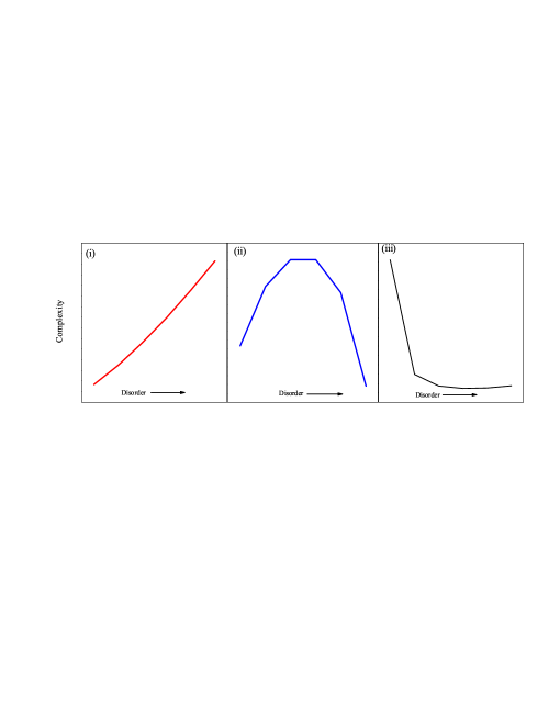
Figure 1.: Three different categories of Complexities, as functions of disorder.

3.3. Fisher information ($I$)

The idea of entropy can adequately explain the degree of disorder of a given phenomenon. Apart from that, however, it is necessary to find out a suitable measure of disorder whose variation derives the event. The concept of entropy is not able to do this. However, $I$ can serve as a good candidate in this context, having the ability to estimate a parameter. Hence it becomes a cornerstone of the statistical field of study, called parameter estimation [126]. $I$ measures the expected error in a smart measurement. Let $e^{2}$ be the mean-square error in an estimation of $\hat{\theta}$ then it obeys the relation,

$$e^{2}I\geq 1;\ \ \ \ I\geq\frac{1}{e^{2}}.$$ (60)

Equation (60) suggests that, $I$ is always greater than the reciprocal of $e^{2}$; only in case of Gaussian distribution it becomes equal to inverse of $e^{2}$. The general form of $I$ is,

$$I=\int\frac{|\nabla\rho(\tau)|^{2}}{\rho(\tau)}\mathrm{d}\tau,$$ (61)

which is a gradient functional of density, measuring the local density fluctuation in a given space. In case of a sharp distribution $I$ is higher; whereas, for a flat distribution it is lower. Thus, it can be concluded that, with a rise in uncertainty, $I$ decreases. It resembles the Weizsäcker kinetic energy functional, $T_{\omega}[\rho]$ often used in DFT [127, 104].

In case of a central potential $I_{\mathrm{\mathbf{r}}}$ and $I_{\mathrm{\mathbf{p}}}$, the net Fisher information, in $\mathrm{\mathbf{r}}$ and $\mathrm{\mathbf{p}}$ spaces respectively, are expressed as [128],

$$I_{\mathrm{\mathbf{r}}}=\int_{{\mathcal{R}}^{3}}\left[\frac{|\nabla\rho(\mathrm{\mathbf{r}})|^{2}}{\rho(\mathrm{\mathbf{r}})}\right]\mathrm{d}\mathrm{\mathbf{r}}=4\langle p^{2}\rangle-2(2l+1)|m|\langle r^{-2}\rangle$$ (62)

$$I_{\mathrm{\mathbf{p}}}=\int_{{\mathcal{R}}^{3}}\left[\frac{|\nabla\Pi(\mathrm{\mathbf{p}})|^{2}}{\Pi(\mathrm{\mathbf{p}})}\right]\mathrm{d}\mathrm{\mathbf{p}}=4\langle r^{2}\rangle-2(2l+1)|m|\langle p^{-2}\rangle,$$

$$\langle r^{2}\rangle=\int_{0}^{r_{c}}\psi_{n_{r},l}^{*}(r)r^{4}\ \psi_{n_{r},l}(r)\mathrm{d}r,\ \ \ \ \ \langle p^{2}\rangle=\int_{0}^{r_{c}}\psi_{n_{r},l}^{*}(r)[-\nabla^{2}\psi_{n_{r},l}(r)]r^{2}\mathrm{d}r$$

$$\left\langle\frac{1}{r^{2}}\right\rangle=\int_{0}^{r_{c}}\psi_{n_{r},l}^{*}(r)\psi_{n_{r},l}(r)\mathrm{d}r,\ \ \ \ \ \left\langle\frac{1}{p^{2}}\right\rangle=\int_{0}^{r_{c}}\psi_{n_{r},l}^{*}(p)\psi_{n_{r},l}(p)\mathrm{d}p.$$

The above equations can be further recast in following equivalent forms [129, 130],

$$I_{\mathrm{\mathbf{r}}} =8\mathcal{E}_{n,l}-8\langle v(r)\rangle-2(2l+1)|m|\langle r^{-2}\rangle$$ (63)

$$I_{\mathrm{\mathbf{p}}} =8\mathcal{E}_{n,l}-8\langle T\rangle-2(2l+1)|m|\langle p^{-2}\rangle$$

$$=\frac{8}{\omega^{2}}\langle v(r)\rangle-2(2l+1)|m|\langle p^{-2}\rangle,$$

where $v(p)$ is the $p$-space counterpart of $v(r)$.

In case of a 3DCHO, $I$’s in $r$ and $p$ space can be expressed analytically as [131],

$$I_{\mathrm{\mathbf{r}}}(\omega)=\frac{\omega}{\sqrt{2}}I_{\mathrm{\mathbf{r}}}(\omega=1),\hskip 8.53581pt\ \ \ \ I_{\mathrm{\mathbf{p}}}(\omega)=\frac{\sqrt{2}}{\omega}I_{\mathrm{\mathbf{p}}}(\omega=1).$$ (64)

Thus, an increase in $\omega$ leads to rise in $I_{\mathrm{\mathbf{r}}}(\omega)$ and fall in $I_{\mathrm{\mathbf{p}}}(\omega)$. However, it is obvious that $I_{t}\ (=I_{\mathrm{\mathbf{r}}}I_{\mathrm{\mathbf{p}}})$ remains invariant with $\omega$. Throughout the article, for brevity, $I_{\mathrm{\mathbf{r}}}(\omega=1)$ and $I_{\mathrm{\mathbf{p}}}(\omega=1)$ will be symbolized as $I_{\mathrm{\mathbf{r}}}$, $I_{\mathrm{\mathbf{p}}}$ respectively.

When $m=0$, $I_{\mathrm{\mathbf{r}}}$ and $I_{\mathrm{\mathbf{p}}}$ in Eq. (62) reduce to further simplified forms as below,

$$I_{\mathrm{\mathbf{r}}}=4\langle p^{2}\rangle,\hskip 8.53581pt\ \ \ \ I_{\mathrm{\mathbf{p}}}=4\langle r^{2}\rangle.$$ (65)

It is seen that, at fixed $n_{r},l$, both $I_{\mathrm{\mathbf{r}}},I_{\mathrm{\mathbf{p}}}$ provide maximum values when $m=0$, and both of them decrease with rise in $m$. Hence one obtains the following upper bound for $I_{t}$,

$$I_{\mathrm{\mathbf{r}}}I_{\mathrm{\mathbf{p}}}\ (=I_{t})\leq 16\langle r^{2}\rangle\langle p^{2}\rangle.$$ (66)

Further adjustment using Eq. (65) leads to following uncertainty relations [128],

$$\frac{81}{\langle r^{2}\rangle\langle p^{2}\rangle}\leq I_{\mathrm{\mathbf{r}}}I_{\mathrm{\mathbf{p}}}\leq 16\langle r^{2}\rangle\langle p^{2}\rangle.$$ (67)

Therefore, in a central potential, $I$-based uncertainty product is bounded by both upper as well as lower limits. They are state-dependent, varying with $n_{r}$ and $l$ quantum numbers.

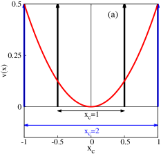
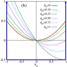
Figure 2.: Schematic representation of a confined 1DQHO potential: (a) SCHO at two separate box lengths (b) ACHO at six chosen values of $d_{m}$ [132].

3.4. Onicescu energy ($E$)

Information energy is the counterpart of information entropy. In 1966, Onicescu defined this quantity as [133],

$$E=\sum_{i}p_{i}^{2}.$$ (68)

It is interesting to note that, in case of a certain event $E$ is maximum. On the contrary, for an equiprobable distribution it is minimum [134, 127, 135]. Qualitatively it is inverse of $S$. When $S$ increases, $E$ decreases and vise-versa. In case of continuous probability distribution, $E$ is an expectation value of probability density. Its mathematical form is,

$$E=\int\rho^{2}(\tau)\ \mathrm{d}\tau.$$ (69)

In addition, Disequilibrium ($D_{e}$) for a continuous probability distribution is defined as,

$$De=\int_{-\infty}^{+\infty}\rho^{2}(\tau)\mathrm{d}\tau.$$ (70)

Therefore, in this occasion, disequilibrium and information energy have same form. Like the previous measures, it is also utilized in orbital-free DFT [105], testing normality [136], electron correlation [110], Colin conjecture [100, 101], configuration interaction [137] etc.

By definition, $E$ refers to the 2nd-order entropic moment [127]; for central potential it assumes the form ($E_{t}$ is the Onicescu energy product),

$$E_{r} =\int_{0}^{\infty}[\rho(r)]^{2}r^{2}\mathrm{d}r,\ \ E_{p}=\int_{0}^{\infty}[\Pi(p)]^{2}p^{2}\mathrm{d}p,$$ (71)

$$E_{\theta,\phi} =\int_{0}^{\pi}[\chi(\theta)]^{2}\sin\theta\mathrm{d}\theta.\ \ E_{t}=E_{r}E_{p}E_{\theta,\phi}^{2}.$$

Uncertainty product for such measures are studied in [138].

3.5. Complexities

In a system, statistical complexity arises due to breakdown of symmetry. It illustrates a competing effect of two complementary quantities, offering a qualitative idea of the organization, structure and correlation. According to [139] it can be broadly characterized into three categories: (i) advances monotonically with disorder (ii) reaches its minimal value for both completely ordered and disordered systems, and a maximum at some intermediate level (iii) increases with order. It has finite value in a state lying between two limiting cases of complete order (maximum distance from equilibrium) and maximum disorder (at equilibrium). Figure 1 pictorially demonstrates above three different kind of complexities as a function of disorder.

The statistical measure of complexity ($C_{LMC}$) is nothing but the product of the information content ($H$) (such as $S$, $R$ etc.) and concentration of spatial distribution ($D$), and can be written as $C_{LMC}=H.D$. This was later criticized [140] and modified [141] to the form of $C_{LMC}=D.e^{S}$, in order to satisfy few conditions such as reaching minimal values for both extremely ordered and disordered limits, invariance under scaling, translation and replication. Various definitions were put forth in literature. Some notable ones include Shiner, Davidson and Landsberg (SDL) [142, 139], Fisher-Shannon $(C_{IS})$ [143, 144, 145], Cramér-Rao [145, 146], generalized Rényi-like [147, 148, 149] complexity, etc. Amongst these, $C_{IS}$ corresponds to a measure which probes a system in terms of complementary global and local factors, and also satisfies certain desirable properties in complexity [127], like invariance under translations and re-scaling transformations, invariance under replication, near-continuity, etc. This has remarkable applications in the study of atomic shell structure, ionization processes [144, 145, 150], as well as in molecular properties like energy, ionization potential, hardness, dipole moment in the localization-delocalization plane showing chemically significant pattern [151], molecular reactivity studies [152]. Some elementary chemical reactions such as hydrogenic-abstraction reaction [153], identity $SN^{2}$ exchange reaction [154], and also concurrent phenomena occurring at the transition region [155] of these reactions have been investigated through composite information-theoretic measures in conjugate spaces.

Without any loss of generality, let us define complexity in following general form $C=Ae^{b.B}$. The order ($A$) and disorder parameters ($B$) may include ($E,I$) and ($R,S$) respectively. With this in mind, we are interested in the following four quantities,

$$C_{ER} =Ee^{bR},\ \ \ \ \ \ \ \ C_{IR}=Ie^{bR},\ \ \ \ \ \ \ C_{ES} =Ee^{bS},\ \ \ \ \ \ \ \ C_{IS}=Ie^{bS}.$$ (72)

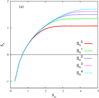
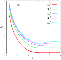
Figure 3.: Plot of (a) $S_{x}$ (b) $S_{p}$, of SCHO potential, as function of $x_{c}$, for first five states [132].

3.6. Relative information

Kullback-Leibler divergence or relative entropy is a descriptor or quantifier of how a measured probability distribution function deviates from a given reference distribution [156, 157]. In quantum mechanics, this characterizes a measure of distinguishability between two states. It actually quantifies the change of information from one state to other [126]. Relative $R$ and $S$ was explored for various atomic systems using H atom ground state as reference [158]. A detailed investigation reveals that, they are directly related with atomic radii and quantum capacitance [159, 158]. Another interesting measure is the relative Fisher information (IR) [160]. It has importance in different topics of physics and chemistry, such as to calculate phase-space gradient of dissipated work and information [161], deriving Jensen divergence [162], relation with score function [163], in the context of study of probability current [164], in thermodynamics [165], etc. Of late it has been successfully used in formulating atomic densities [166] and deriving density functionals under local-density and generalized-gradient approximations [167]. Further, IR along with Hellmann-Feynman and virial theorem has been used to develop a Legendre transform structure related to SE [168]. It has been designed self-consistently on the basis of estimation theory [169]. In quantum chemistry perspective, it has been successfully formulated using above two theorems and entropy maximization principle [170, 171, 172]. Very recently, IR for some exactly solvable potentials including 1D and 3D QHO in both position and momentum spaces has been estimated analytically using ground state of definite symmetry (for example, $l=0$ for $s$ orbitals, $l=1$ for $p$ orbital, and so on) as reference [173]. Before that, a numerical estimation of IR in position space is done for H-atom using $1s$ orbital as basis [174].

For two normalized probability densities $\rho_{n,l,m}(\tau),\rho_{n_{1},l_{1},m_{1}}(\tau)$, IR is expressed as,

$$\mathrm{IR}\ [\rho_{n,l,m}(\tau)|\rho_{n_{1},l_{1},m_{1}}(\tau)]=\int_{{\mathcal{R}}^{3}}\rho_{n,l,m}(\tau)\left|\nabla\ \mathrm{ln}\left\{\frac{\rho_{n,l,m}(\tau)}{\rho_{n_{1},l_{1},m_{1}}(\tau)}\right\}\right|^{2}\mathrm{d}\tau.$$ (73)

Here $n,l,m$ and $n_{1},l_{1},m_{1}$ are the descriptors of target and reference states respectively, while $\tau$ is a generalized variable. In case of central potential, these probability densities $\rho_{n,l,m}(\tau)$, $\rho_{n_{1},l_{1},m_{1}}(\tau)$ can be expressed in following forms, without any loss of generality,

$$\rho_{n,l,m}(\tau) =R_{n,l}^{2}(s)\Theta_{l,m}^{2}(\theta);\ \hskip 8.53581pt\rho_{n_{1},l_{1},m_{1}}(\tau)=R_{n_{1},l_{1}}^{2}(s)\Theta_{l_{1},m_{1}}^{2}(\theta).$$ (74)

In the above equation, $R_{n,l}(s),R_{n_{1},l_{1}}(s)$ signify radial parts, $\Theta_{n,l}(\theta),\Theta_{n_{1},l_{1}}(\theta)$ represent angular contributions of two wave functions, whereas $``s"$ implies either $r$ or $p$ variable in respective radial functions. Thus Eq. (73) may be rewritten as,

$$\mathrm{IR}\ [\rho_{n,l,m}(\tau)|\rho_{n_{1},l_{1},m_{1}}(\tau)]=\mathrm{IR}\ [\rho_{n,l}(s)|\rho_{n_{1},l_{1}}(s)]+\left\langle\frac{1}{s^{2}}\right\rangle\mathrm{IR}\ [\Theta_{l,m}^{2}(\theta)|\Theta_{l_{1},m_{1}}^{2}(\theta)]+\\ 2\int_{0}^{\infty}s~{}R_{n,l}^{2}(s)\left[\frac{d}{ds}\mathrm{\ln}\left\{\frac{R^{2}_{n,l}(s)}{R^{2}_{n_{1},l_{1}}(s)}\right\}\right]\mathrm{d}s\int_{0}^{\pi}\Theta_{l,m}^{2}(\theta)\left[\frac{d}{d\theta}\mathrm{ln}\left\{\frac{\Theta_{l,m}^{2}(\theta)}{\Theta_{l_{1},m_{1}}^{2}(\theta)}\right\}\right]\sin\theta\mathrm{d}\theta$$ (75)

where the following quantities have been defined,

$$\mathrm{IR}\ [\rho_{n,l}(s)|\rho_{n_{1},l_{1}}(s)] =\int_{0}^{\infty}s^{2}~{}\rho_{n,l}(s)\left|\frac{d}{ds}\mathrm{ln}\left\{\frac{\rho_{n,l}(s)}{\rho_{n_{1},l_{1}}(s)}\right\}\right|^{2}\mathrm{d}s$$ (76)

$$\mathrm{IR}\ [\Theta_{l,m}^{2}(\theta)|\Theta_{l_{1},m_{1}}^{2}(\theta)] =\int_{0}^{\pi}\Theta_{l,m}^{2}(\theta)\left|\frac{d}{d\theta}\mathrm{ln}\left\{\frac{\Theta_{l,m}^{2}(\theta)}{\Theta_{l_{1},m_{1}}^{2}(\theta)}\right\}\right|^{2}\sin\theta~{}\mathrm{d}\theta$$

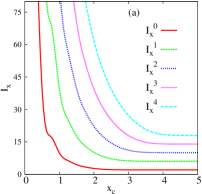
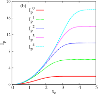
Figure 4.: Plot of $I_{x}$, $I_{p}$, $E_{x}$, $E_{p}$ for first five states of SCHO potential, as functions of $x_{c}$, in panels (a), (b), (c) and (d). See text for details [132].

4. Result and Discussion

4.1. 1D Confined harmonic oscillator (1DCHO)

Panel (a) of Fig. 2 represents an SCHO scenario for two box lengths $1$ and $2$, respectively. Next, the asymmetric confinement in a 1DQHO can be invoked in two different ways: (i) by varying the box boundary, keeping box length and $d_{m}$ fixed at zero (ii) the other way is to change $d_{m}$ by keeping box length and boundary constant. We have chosen the second option; where a rise in $d_{m}$ transfers the minimum towards the right of origin, keeping box length, $b_{2}-b_{1}=2$ fixed, while left and right boundaries are residing at $b_{1}=-1$ and $b_{2}=1$. Moreover, since $\frac{1}{2}k(x\pm d_{m})^{2}$ illustrates a mirror-image pair potential trapped within $b_{1}$ and $b_{2}$, their eigenvalues and expectation values are same for all states. As the respective wave functions are mirror images of each other, it suffices to consider the behavior of either one of them. The other one automatically follows from it. The right-hand panel (b) of Fig. 1 shows a schematic representation of an ACHO potential, at five different $d_{m}$ values.

Table 3.: Comparison of energies of first six states of ACHO potential at four distinct $d_{m}$. Length of the box is fixed at 2. PR implies Present Result [132]. See text for details.

$d_{m}$	$\epsilon_{0}$ (PR)	$\epsilon_{0}$ (Ref.)	$\epsilon_{1}$ (PR)	$\epsilon_{1}$(Ref.)
0.36	2.7177633960054	2.7177633960054${}^{\ddagger}$	10.283146010610	10.283146010610${}^{\ddagger}$
1.92	6.0383021056781	6.0383021056781${}^{\ddagger}$	13.901445986629	13.901445986629${}^{\ddagger}$
5.00	26.065225076406	26.065225076406${}^{\ddagger}$	35.462261039378	35.462261039378${}^{\ddagger}$
10.0	97.474035270680	97.474035270680${}^{\ddagger}$	110.51944554927	110.51944554927${}^{\ddagger}$
	$\epsilon_{2}$ (PR)	$\epsilon_{2}$ (Ref.)	$\epsilon_{3}$ (PR)	$\epsilon_{3}$(Ref.)
0.36	22.648848755052	22.648848755052${}^{\ddagger}$	39.929984298830	39.929984298830${}^{\ddagger}$
1.92	26.249310409373	26.249310409373${}^{\ddagger}$	43.513981920357	43.513981920357${}^{\ddagger}$
5.00	47.817024422796	47.817024422796${}^{\ddagger}$	64.900200447511	64.900200447511${}^{\ddagger}$
10.0	123.593144939095	123.593144939095${}^{\ddagger}$	140.555432078323	140.555432078323${}^{\ddagger}$
	$\epsilon_{4}$ (PR)	$\epsilon_{4}$ (Ref.)	$\epsilon_{5}$ (PR)	$\epsilon_{5}$(Ref.)
0.36	62.140768627508	62.140768627508${}^{\ddagger}$	89.284409553063	89.284409553063${}^{\ddagger}$
1.92	65.715672311936	65.715672311936${}^{\ddagger}$	92.854029622882	92.854029622882${}^{\ddagger}$
5.00	87.137790461503	87.137790461503${}^{\ddagger}$	114.244486402564	114.244486402564${}^{\ddagger}$
10.0	162.519960161732	162.519960161732${}^{\ddagger}$	189.515389275133	189.515389275133${}^{\ddagger}$

${}^{\ddagger}$ITP result [34].

4.1.1. Symmetrically confined harmonic oscillator (SCHO)

In this case, all calculations are performed involving the wave function given in Eq. (2). Figure 3 shows plots of $S_{x}$, $S_{p}$ versus $x_{c}$, for first five states of SCHO. In panel (a), $S_{x}$ progresses with box length and converges to a constant value ($S_{x}$ of 1DQHO) at sufficiently large box length. At small $x_{c}$ region, $S_{x}$ changes rather insignificantly with $n$, corresponding to the behavior of a PIB problem (where $S_{x}$ remains unchanged with $n$). Next, panel (b), imprints that $S_{p}$ abates with increase in box length and finally merges to corresponding 1DQHO value. It is important to note that, there appears a minimum in $S_{p}$ for all excited states. Appearance of such minimum may be ascribed to the competing effect in $p$ space. In fact, three possibilities could be contemplated ($l_{x}$, $l_{p}$ are box lengths in $x$, $p$ space):

1. When $l_{x}\rightarrow 0,$ then $l_{p}\rightarrow\infty$.

2. When $l_{x}$ is finite, then $l_{p}$ is also finite. But an increase in $l_{x}$ leads to a decrease in $l_{p}$.

3. When $l_{x}\rightarrow\infty,$ then also $l_{p}\rightarrow\infty$.

These plots suggest that, at the beginning, with increase in $l_{x}$, particle gets localized in $p$ space ($S_{p}$ decreases), but when potential behaves like 1DQHO, de-localization predominates. Thus, existence of minimum in $S_{p}$ is due to presence of two conjugate forces. These variations of $S_{x}$, $S_{p}$ with $x_{c}$ are in complete agreement with the findings of [175].

The behavior of $I_{x}$, $I_{p}$ with respect to $x_{c}$ of first five stationary states are exhibited in two bottom panels (a), (b) of Fig. (4). One can see that initially $I_{x}$ decreases sharply, extent of which is maximum for the lowest state and successively decreases with $n$. Then it attains a constant value after a certain $x_{c}$. On the contrary, in panel (b), $I_{p}$ strongly grows with $x_{c}$ at first; the extent increases with $n$, lowest state producing lowest. Finally, for all states, it eventually reaches a state-dependent constant value as in $I_{x}$. It is pertinent to mention that, behavior of $I_{x}$, $I_{p}$ under confinement agrees with those of $\Delta p$, $\Delta x$ [175]. Next, panel (c) reveals that, $E_{x}$ for all these states remain very close to each other at smaller $x_{c}$; then as $x_{c}$ progresses, $E_{x}$ for individual states branch out and decreases indicating delocalization. In the end, it reaches some constant value for all $n$. Lastly, in panel (d), $E_{p}$s tend to advance in the beginning for all states at low $x_{c}$ region, eventually becoming smooth after some threshold $x_{c}$. These calculation have further consolidated the conclusions obtained from the study of $S_{x}$, $S_{p}$, $S$ demonstrated earlier.

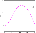
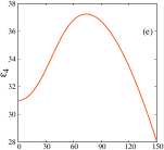
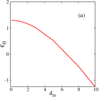
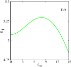
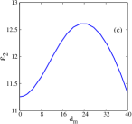
Figure 5.: Variation of $\epsilon_{n}$ ($n\!=\!0-5$) of ACHO potential as function of $d_{m}$ [132].

4.1.2. Asymmetrically confined harmonic oscillator (ACHO)

Now, the focus is on the ACHO case. This presentation is based on results of $\epsilon_{n}$; $S_{x},S_{p}$; $I_{x},I_{p}$; $E_{x},E_{p}$ as functions of $d_{m}$, for some low-lying states. Throughout the whole presentation, the box length has been kept fixed at 2 and boundaries are placed at $-$1 and 1. At the outset it is important to note that, an increase in $d_{m}$ leads to localization in real space. Thus it can be expected that, there will be delocalization in $p$ space.

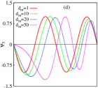
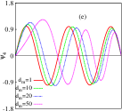
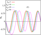
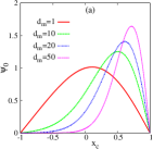
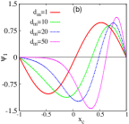
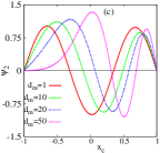
Figure 6.: Wave functions of lowest six states of ACHO potential at four specific values of $d_{m}$, namely 1, 10, 20, 50. Panels (a)–(f) represent $n\!=\!0-5$ states [132]. See text for details.

Before looking into the behavior of IE in ACHO, it is pertinent to make some comments about its eigenvalues and eigenfunctions. ACHO has been studied using power-series solution [32] and ITP method [34]. In this section, we shall, however, present another simple method, which produces quite accurate results. In this variation induced exact diagonalization procedure [176], an energy functional is minimized using an SCHO basis set. Recently this method has been successfully employed in studying symmetric and asymmetric double-well potentials [177, 178], where a 1DQHO basis was utilized.

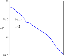
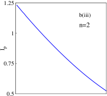
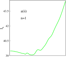
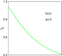
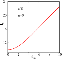
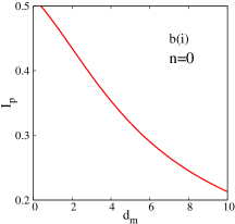
Figure 7.: Plot of $I_{x}$, $I_{p}$, $I$ of first five states of ACHO potential, as function of $d_{m}$, in left (a), middle (b), right (c) columns; (i)–(iii) represent $n=0-2$ states [132]. See text for details.

The Hamiltonian matrix elements are evaluated by using functions given in Eq. (2). Presence of a single non-linear parameter $\alpha$ allows us to adopt a coupled variation procedure. Further it is easy to confirm the convergence of results with respect to basis dimension $N$. Thus it provides a secular equation at each $\alpha$. The kinetic energy part blows up to $\infty$ when $\alpha\rightarrow\infty$, whereas at $\alpha\rightarrow 0$, potential energy part behaves in a similar fashion. This qualitative analysis through uncertainty principle, confirms the existence of such basis. Diagonalization of $H_{mn}=\langle m|\hat{H}|n\rangle$ leads to accurate eigenvalues and eigenfunctions, which is attained through MATHEMATICA package. In principle, to achieve exact solution, one needs to employ the complete basis; however for practical purposes a truncated basis of finite dimension is envisaged. Here, $N=50$ appears adequate; with further increase in basis, result improves. A cross-section of energies obtained from above scheme is produced in Table 3, for lowest six states of ACHO at four selected $d_{m}$. Some literature results are provided for comparison, wherever available. For all four $d_{m}$, present energies with SCHO basis, practically coincide with ITP results [34], for all digits reported. It is expected that this SCHO basis may be useful in future for other confined and free 1D potentials.

Our calculated ACHO energies of Table 3 are presented in Fig. 5, for first six states with respect to $d_{m}$, in panels (a)-(f). Ranges of $\epsilon_{n}$ and $d_{m}$ are different for each $n$. Variation in $\epsilon_{0}$ is unique amongst all $\epsilon_{n}$, where, from an initial higher value at small $d_{m}$, ground-state energy continuously falls. In all excited states, however, it passes through a maximum; with increase in $n$, this maximum shifts to higher values of $d_{m}$. Next Fig. 6 portrays our computed wave functions for $n\!=\!0-5$ states of ACHO at four selected $d_{m}$ values. Clearly, the maximum, minimum and nodal positions of all $\psi_{n}$’s switch towards right with advancement in $d_{m}$. These plots suggest that particle gets localized in $x$ space as $d_{m}$ progresses.

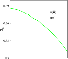
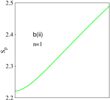
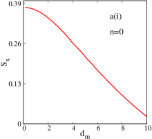
Figure 8.: Plot of $S_{x}$, $S_{p}$, $S$ of first three states of ACHO potential, as function of $d_{m}$, in left (a), middle (b), right (c) columns; (i)–(iii) represent $n=0-2$ states [132]. See text for details.

Now we move on to $I_{x},I_{p}$ variations with change of $d_{m}$. These are shown pictorially in Fig. 7 left (a), and right (b) panels display these in conjugate $x$, $p$ spaces respectively. For ground and first excited state $I_{x}$ tends to increase with $d_{m}$, on the whole, whereas for ($n=2$) state, the same decreases. Thus, for first two states, it indicates localization in $x$ space and delocalization for 2nd excited state. A careful investigation of panels b(i)–b(iii) of Fig. 7 reveals that, $I_{p}$, for all $n$ under consideration, consistently decreases with increase of $d_{m}$, signifying a delocalization of particle in $p$ space.

Next, it is imperative to explore changes in behavior of $S_{x},S_{p}$ with respect to $d_{m}$. These are offered in Fig. 8. It is clear from left panels a(i)–a(iii) of Fig. 8 that, $S_{x}$ for all these three states generally decreases monotonically with growth in $d_{m}$, signifying localization of particle in position space. Likewise, a scrutiny of right plots b(i)–b(iii) of Fig. 8 summarizes an opposite trend in $S_{p}$ with increase in $d_{m}$. A sample of $S_{x},S_{p}$ are reported in Table 4 for $n\!=\!0,1,2$ states at five selected $d_{m}$ values, namely, 0.12, 2.04, 5, 7 and 10. Evidently, these entries corroborate the outcomes of Fig. 8.

Now, we move on to an analysis of $E$, using Fig. 9, for $n=0-2$. Panels a(i)–a(iii) suggest that, for all three states there is an overall increase of $E_{x}$ with rise in $d_{m}$. This indicates localization in $x$ space. Panels b(i)–b(iii) portray that, general trend of $E_{p}$ is a gradual decrease with rise in $d_{m}$.

On the basis of above discussion, it is clear that, only $S_{x},S_{p}$ can adequately explain localization-delocalization phenomena in an ACHO. Study of $E_{x},E_{p}$ can also offer valuable knowledge about the dual nature of $E$ in composite $x$, $p$ space. But, $I_{x},I_{p}$ appear to be inadequate in explaining the contrasting phenomena in ACHO.

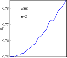
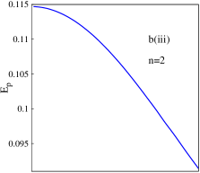
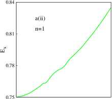
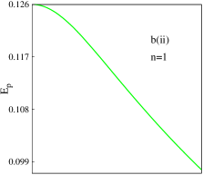
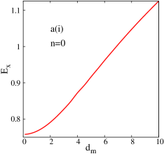
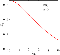
Figure 9.: Plot of $E_{x}$, $E_{p}$, $E$ of first three states of ACHO potential, as function of $d_{m}$, in left (a), middle (b), right (c) columns; (i)–(iii) represent $n=0-2$ states [132]. See text for details.

4.2. 3D Confined harmonic oscillator (3DCHO)

At the onset, it is convenient to point out that, net information measures in conjugate $r$ and $p$ space may be segmented into radial and angular parts. In a given space, the results provided correspond to net measures including the angular contributions. One can transform the 3DQHO into a 3DCHO by squeezing the radial boundary of former from infinity to a finite region. This alteration in radial environment does not affect the angular boundary conditions. Therefore, angular part of the information measures in free and confined systems remain unchanged in both spaces. Further as we are solely focused in radial confinement, this will also not influence the characteristics of a given measure as one changes $r_{c}$. Throughout this investigation, magnetic quantum number $m$ remains fixed to $0$ for $R,S,E$ calculation. However, $I$ has been studied for non-zero $m$ states. The radial wave function in $r$ and $p$ spaces depend only on $n_{r},l$ quantum numbers. Hence, in both space, radial wave function can be obtained by considering $m=0$. Further, a change in $m$ from zero to non-zero value will not influence the expression of radial wave function in $p$ space. Also note that, we have followed the spectroscopic notation, i.e., the levels are denoted by $n_{r}+1$ and $l$ values (see, e.g., [69]). Therefore, $n_{r}=0$ and $l=4$ signifies $1g$ state. The radial quantum number $n_{r}$ relates to $n$ as $n=2n_{r}+l$.

Table 4.: $S_{x},S_{p},S$ for $n\!=\!0-2$ states of ACHO at five specific $d_{m}$ [132]. See text for details.

$d_{m}$	$S_{x}^{0}$	$S_{p}^{0}$	$S^{0}$	$S_{x}^{1}$	$S_{p}^{1}$	$S^{1}$	$S_{x}^{2}$	$S_{p}^{2}$	$S^{2}$
0.12	0.3783	1.8296	2.2079	0.3857	2.2212	2.6069	0.3862	2.3692	2.7554
2.04	0.3428	1.8779	2.2208	0.3807	2.2512	2.6319	0.3850	2.3852	2.7703
5.0	0.2184	2.0238	2.2422	0.3636	2.3390	2.7027	0.3782	2.4512	2.8295
8.0	0.093	2.1576	2.2506	0.3360	2.4313	2.7674	0.3695	2.5429	2.9124
10.0	0.0233	2.2294	2.2527	0.3108	2.4900	2.8009	0.3611	2.6057	2.9668

$I_{\mathrm{\mathbf{r}}},I_{\mathrm{\mathbf{p}}}$ values are obtained from Eq. (62). In all occasions, it has been verified that, in both spaces, as $r_{c}\rightarrow\infty$, $I_{\mathrm{\mathbf{r}}}$ and $I_{\mathrm{\mathbf{p}}}$ merge to respective 3DQHO limit. The net $I$ in $r$ and $p$ spaces are divided into radial and angular part. But in both $I_{\mathrm{\mathbf{r}}}$ and $I_{\mathrm{\mathbf{p}}}$ expressions, angular contribution is normalized to unity. Hence, evaluation of all these targeted quantities using only radial part will serve our purpose. Pilot calculations are done for $1s$-$1g$ and $2s$-$2m$ states, with $r_{c}$ varying from 0.1 to 7 a.u. The former set is chosen as they represent node-less ground states corresponding to various $l$, whereas, $2s$-$2m$ states are considered to perceive the effect of nodes on $I$ at non-zero $m$.

It is worthwhile noting that, $I$’s can be accurately calculated from a knowledge of $\langle p^{2}\rangle,\left\langle\frac{1}{r^{2}}\right\rangle,\langle r^{2}\rangle,\left\langle\frac{1}{p^{2}}\right\rangle$. Two possibilities may be invoked: (i) first three quantities evaluated in $r$ space, while $\langle p^{-2}\rangle$ in $p$ space (ii) $\langle r^{2}\rangle,\langle r^{-2}\rangle$ in $r$ space, while $\langle p^{2}\rangle,\langle p^{-2}\rangle$ in $p$ space. Here we have opted for first route removing the necessity to do numerical differentiation in either spaces. This has been discussed in detail in a recent article [97].

Exact analytical form of $I_{\mathrm{\mathbf{r}}}$ and $I_{\mathrm{\mathbf{p}}}$ in isotropic 3DQHO was given in [128],

$$I_{\mathrm{\mathbf{r}}}(\omega)=4\omega\left(2n_{r}+l-|m|+\frac{3}{2}\right),\ \ \ I_{\mathrm{\mathbf{p}}}(\omega)=\frac{4}{\omega}\left(2n_{r}+l-|m|+\frac{3}{2}\right).$$ (77)

Thus, at a certain $m$, both $I_{\mathrm{\mathbf{r}}}(\omega),I_{\mathrm{\mathbf{p}}}(\omega)$ increase as $n_{r}$ and $l$ approach higher values. Similarly, for specific $n_{r}$ and $l$, both $I_{\mathrm{\mathbf{r}}}(\omega),I_{\mathrm{\mathbf{p}}}(\omega)$ regress with growth in $|m|$. Effect of $\omega$ on $I_{\mathrm{\mathbf{r}}}(\omega),I_{\mathrm{\mathbf{p}}}(\omega)$ is quite straightforward. $I_{\mathrm{\mathbf{r}}}(\omega)$ advances and $I_{\mathrm{\mathbf{p}}}(\omega)$ decreases with rise of $\omega$. By putting $\omega=1$ in Eq. (77) one easily recovers expressions for $I_{\mathrm{\mathbf{r}}},I_{\mathrm{\mathbf{p}}}$ in a 3DQHO.

Table 5.: $\mathcal{E}_{n_{r},l}(n_{r}=0)$ of lowest five circular states of 3DCHO, PISB at five $r_{c}$, from [34, 130].

$l$	$r_{c}=0.01$	$r_{c}=0.05$	$r_{c}=0.1$	$r_{c}=0.2$	$r_{c}=0.5$
3DCHO
0	49348.02202373	1973.92123372	493.48163345	123.37570844	19.77453418
1	100953.64280465	4038.14617967	1009.53830088	252.39159906	40.42827649
2	166087.30959293	6643.49293120	1660.87528919	415.22704789	66.48975653
3	244155.96823805	9753.60193720	2441.56211674	610.39965899	97.72324914
4	334771.55964446	13390.86304096	3347.71822121	836.93939916	133.97424683
PISB
0	49348.022005446	1973.92088021	493.48022005	123.37005501	19.73920880
1	100953.64278213	4038.14571128	1009.53642782	252.38410695	40.38145711
2	166087.30957134	6643.49238285	1660.87309571	415.21827392	66.43492382
3	244155.96821809	9753.60153136	2441.55968218	610.38992054	97.66238728
4	334771.55962552	13390.86238502	3347.71559625	836.92889906	133.90862385

At first we illustrate the behavior of 3DCHO at $r_{c}\rightarrow 0$. A diligent study reveals that, at small $r_{c}$ region, 3DCHO has an energy spectrum comparable to that of a particle in a spherical box (PISB). This leaning generally holds good for all other states as well. A cross-section of eigenvalues ($1s$-$1g$) of lowest five circular states corresponding to $l=0$-4, of 3DCHO and PISB, given in Table 5, at five selected $r_{c}$, viz., $0.01,0.05,0.1,0.2,0.5$, supports this fact. However this observation should not be misinterpreted to conclude that at $r_{c}\rightarrow 0$, 3DCHO leads to PISB. Because that can happen only when both systems have nearly equal kinetic energy as well as potential energy components. This is not apparent from this table. At this point, it is noteworthy to mention that, like 3DCHO, PISB is also exactly solvable; eigenfunctions are explicable directly in terms of first-order Bessel function, and given as,

$$J_{l}(Z)=(-1)^{l}Z^{l}\left(\frac{1}{Z}\frac{d}{dZ}\right)^{l}\left(\frac{\sin{Z}}{Z}\right),\\$$ (78)

where $Z=\sqrt{\mathcal{E}_{n_{r},l}}\ r$. At the boundary when $r=r_{c}$, $Z=Z_{n_{r},l}$ and $J_{l}(Z_{n_{r},l})=0$. Moreover, at $r=r_{c}$, the energy of a $(n_{r},l)$ state is written as $\mathcal{E}_{n_{r},l}=\frac{Z_{n_{r},l}^{2}}{r_{c}^{2}}$ [179]. This $J_{l}(Z_{n_{r},l})=0$ is a transcendental equation and at a constant $n_{r},l$, this $Z_{n_{r},l}$ is evaluated by the help of MATHEMATICA program package. Thus all the PISB energies in lower segment of this table have been calculated following the above procedure.

Table 6.: $I_{\mathrm{\mathbf{r}}},I_{\mathrm{\mathbf{p}}}$ of lowest five circular states of 3DCHO and PISB at five $r_{c}$ at fixed $m(0)$ [130].

System	$l$	$r_{c}=0.01$	$r_{c}=0.05$	$r_{c}=0.1$	$r_{c}=0.2$	$r_{c}=0.5$
$I_{\mathrm{\mathbf{r}}}$
	0	394784.1761898	15791.36986976	3947.84176	986.960440	157.913740
	1	807629.1424372	32305.16943736	8076.29142	2019.072855	323.05170823
3DCHO	2	1328698.4767434	53147.9434496	13286.984765	3321.7461915	531.4794285
	4	2678172.4771556	107126.9043276	26781.72476	6695.431192	1071.269013
	0	394784.1760435	15791.3670417	3947.8417604	986.9604401	157.9136704
	1	807629.1422570	32305.1656902	8076.2914225	2019.0728556	323.0516569
PISB	2	1328698.4765707	53147.9390628	13286.9847657	3321.7461914	531.4793906
	4	2678172.4770042	107126.8990801	26781.7247700	6695.4311925	1071.2689908
$I_{\mathrm{\mathbf{p}}}$
	0	0.0001130690	0.0028267272	0.011306900	0.0452270673	0.282533301
	1	0.0001498425	0.0037460639	0.014984249	0.0599366038	0.374503742
3DCHO	2	0.0001754798	0.0043869959	0.017547979	0.0701916254	0.438623720
	4	0.0002100025	0.0052500632	0.021000250	0.0840008284	0.524961467
	0	0.0001130690	0.002826727	0.011306909	0.045227638	0.282672741
	1	0.0001498425	0.003746064	0.014984256	0.059937024	0.374606402
PISB	2	0.0001754798	0.004386996	0.017547984	0.070191936	0.438699601
	4	0.0002100025	0.005250063	0.021000253	0.084001012	0.525006325

The upper portion of Table 6 portrays $I_{\mathrm{\mathbf{r}}}$ of 3DCHO and PISB at five selected $r_{c}$ values introduced before; the respective $I_{\mathrm{\mathbf{p}}}$ of two systems are reported in lower portion. It is interesting to point out that, for 3DQHO and 3DCHO in a state having $m=0$, $I_{\mathrm{\mathbf{r}}}$ and $I_{\mathrm{\mathbf{p}}}$ are directly connected to expectation values of kinetic and potential energy as;

$$I_{\mathrm{\mathbf{r}}}(\omega)=8\langle T\rangle,\ \ \ I_{\mathrm{\mathbf{p}}}(\omega)=\frac{8}{\omega^{2}}\langle v(r)\rangle.$$ (79)

But for a PISB, total energy is exclusively kinetic energy as the potential energy is zero. However, one can evaluate $I_{\mathrm{\mathbf{r}}},I_{\mathrm{\mathbf{p}}}$ for PISB and collate the results with 3DCHO. Because, a pair of systems possessing same $I_{\mathrm{\mathbf{r}}},I_{\mathrm{\mathbf{p}}}$ for all states indicate identical physical and chemical environment. Hence, here we have exploited $I$ to investigate the characteristics of PISB and 3DCHO at $r_{c}\rightarrow 0$. The table clearly manifests that at $r_{c}\rightarrow 0$, a 3DCHO has comparable $I_{\mathrm{\mathbf{r}}},I_{\mathrm{\mathbf{p}}}$ values with that of PISB, thus confirming our presumption that, at $r_{c}\rightarrow 0$, 3DCHO behaves like a PISB. One also marks that, with reduction in $r_{c}$, $I_{\mathrm{\mathbf{p}}}$ (and also potential energy) approaches zero. On the other hand, as $r_{c}$ grows, the separation between $I_{\mathrm{\mathbf{r}}}$ (also $I_{\mathrm{\mathbf{p}}}$) values of 3DCHO and PISB tends to increase significantly. Moreover, as expected, at $r_{c}\rightarrow\infty$, 3DCHO reduces to 3DQHO. In previous section it was pointed out that, a 1DCHO may be treated as a two-mode system; at smaller (approaching zero) and larger (tending infinity) confinement lengths it behaving like a particle in a box and an 1DQHO respectively [180, 175]. Here, also we observe resembling behavior. At $r_{c}\rightarrow 0$ and $\infty$, 3DCHO leads to PISB and a 3D isotropic QHO respectively. We also note that, larger the value of $\omega$ higher will be $\langle v(r)\rangle$; as a matter of fact 3DCHO is more prone to 3DQHO in such a case. Conversely, lesser the $\omega$ value, $\langle v(r)\rangle$ is smaller and 3DCHO, in that occasion, is inclined towards a PISB. Therefore at a fixed $r_{c}$, by controlling $\omega$ values one can inquire the properties of all three systems starting from PISB to 3DQHO through 3DCHO.

Table 7.: $I_{\mathrm{\mathbf{r}}},I_{\mathrm{\mathbf{p}}}$ for lowest five $n_{r}$ ($l=0$) values at six different $r_{c}$ [130]. See text for details.

$n_{r}$	$r_{c}=0.1$	$r_{c}=0.5$	$r_{c}=1$	$r_{c}=2$	$r_{c}=7$	$r_{c}=\infty$
$I_{\mathrm{\mathbf{r}}}$
0	3947.84176	157.9137401	39.48285935	10.130828577	6.00000000	6
1	15791.3670	631.654662	157.91245186	39.42241043	14.00000000	14
2	35530.57584	1421.2230213	355.3049651	88.77709457	22.00000000	22
3	63165.46816	2526.6187189	631.6541846	157.88183967	30.00000000	30
4	98696.0440	3947.8417551	986.960106	246.718681361	38.00000000	38
$I_{\mathrm{\mathbf{p}}}$
0	0.0113069007	0.2825333012	1.1217967676	3.9877029335	6.0000000	6
1	0.01282672989	0.32070687721	1.28512015257	5.25470219890	14.0000000	14
2	0.0131081767	0.3277292039	1.3124046596	5.34276239849	22.00000000	22
3	0.0132066828	0.3301825760	1.3216621568	5.3463257844	30.00000000	30
4	0.0132522770	0.33131731951	1.3258940221	5.3437134181	38.00000000	38

So far, we have explored the limiting trend of 3DCHO. Now we look into its behavior at intermediate $r_{c}$ region. For that, at first, the dependence of $I_{\mathrm{\mathbf{r}}},I_{\mathrm{\mathbf{p}}}$ on quantum number $n_{r}$ is recorded in Table 7. It tabulates these quantities for lowest five $n_{r}$ (0-4) at six representative $r_{c}$ values. This clearly implies that, at fixed $m,l$ and $r_{c}$, both $I_{\mathrm{\mathbf{r}}},I_{\mathrm{\mathbf{p}}}$ in 3DCHO get incremented as $n_{r}$ attains higher values. Henceforth, the role of $n_{r}$ on these measures is not discussed any further.

Table 8.: $I_{\mathrm{\mathbf{r}}},I_{\mathrm{\mathbf{p}}}$ of $1p,1d,1f$ states of 3DCHO at six $r_{c}$, with varying $m$. Last column correspond to respective 3DQHO values, computed from Eq. (77) [130].

$|m|$	$r_{c}=0.1$	$r_{c}=0.5$	$r_{c}=1$	$r_{c}=2$	$r_{c}=7$	$r_{c}=\infty$
$I_{\mathrm{\mathbf{r}}}(1p)$
0	8076.29142	323.0517082	80.76619765	20.39764116	10.00000000	10
1	5736.542528	229.4242339	57.21792995	13.91660078	6.00000000	6
$I_{\mathrm{\mathbf{p}}}(1p)$
0	0.014984249	0.374503742	1.491857857	5.577935621	10.00000000	10
1	0.01003	0.2507	0.9980	3.975	6.0000	6
$I_{\mathrm{\mathbf{r}}}(1d)$
0	13286.984765	531.4794285	132.8722779	33.37450170	14.00000000	14
1	10419.849672	416.7666252	104.0908347	25.74558754	10.00000000	10
2	7552.714578	302.0538220	75.3093915	18.11667339	6.00000000	6
$I_{\mathrm{\mathbf{p}}}(1d)$
0	0.017547979	0.43862372	1.74993894	6.70582522	14.0000000	14
1	0.0133333	0.33326	1.32905	5.0595	10.00000	10
2	0.0091187	0.2279	0.9081	3.4132	6.00000	6
$I_{\mathrm{\mathbf{r}}}(1f)$
0	19532.47745	781.2991270	195.3266196	48.95155358	18.000000000	18
1	16156.649498	646.2448005	161.48315319	40.15669405	14.00000000	14
2	12780.8215	511.1904739	127.63968669	31.36183453	10.00000000	10
3	9404.993581	376.1361474	93.79622020	22.566975007	6.000000000	6
$I_{\mathrm{\mathbf{p}}}(1f)$
0	0.0194769435	0.486866098	1.944005783	7.551236509	18.0000000	18
1	0.0157907758	0.39471708	1.57572258	6.0995039	14.00000	14
2	0.012104608	0.30256807	1.20743938	4.6477714	10.00000	10
3	0.008418440	0.2104190	0.8391561	3.196038	6.00000	6

Now, in order to get a clear picture of the effect of magnetic quantum number, Table 8 gives $I_{\mathrm{\mathbf{r}}},I_{\mathrm{\mathbf{p}}}$ of 3DCHO for lowest three nodeless states having $l\neq 0$, i.e., $1p$-$1f$ respectively, for all allowed $m$ at 6 carefully selected $r_{c}$ ($0.1,0.5,1,2,7,\infty$). Likewise, Fig. 10 portrays these for $1g$ state in panels (a) and (b), for all possible $|m|$. It is to be noted that, the quantities in last column at $r_{c}=\infty$ are given from Eq. (77) considering $\omega=1$. For this special $\omega$, Eq. (77) dictates that, $I_{\mathrm{\mathbf{r}}}=I_{\mathrm{\mathbf{p}}}$ for 3DQHO. One notices that, behavior of $I_{\mathrm{\mathbf{r}}}$ and $I_{\mathrm{\mathbf{p}}}$ in 3DCHO is always in agreement with 3DQHO; an explicit analysis suggests identical patterns. In general, $I_{\mathrm{\mathbf{r}}}$ decays monotonically while $I_{\mathrm{\mathbf{p}}}$ progresses with rise in $r_{c}$; this is found to hold true for all $|m|$. This is to be expected, as a growth in $r_{c}$ promotes delocalization in $r$ space and localization in $p$ space. At a fixed $r_{c}$ and fixed quantum numbers $n_{r}$ and $m$, $I_{\mathrm{\mathbf{r}}}$ tends to rise with $l$; this is consistent to what is observed from Eq. (77) in 3DQHO. Because, in both 3DCHO and 3DQHO, kinetic energy grows with $n_{r},l$. Similarly, at fixed $n_{r},l$, in both 3DCHO and 3DQHO, $I_{\mathrm{\mathbf{r}}}$ falls down as one descends down the table (increment in $|m|$). One striking fact is that, for all these three states considered, both 3DCHO and 3DQHO portray comparable pattern with respect to $m$. Next, $I_{t}$ for $1p$-$1f$ states of 3DCHO are offered in Table 9. It seems to show an inclination towards $I_{\mathrm{\mathbf{r}}}$ in the behavioral pattern. In all instances, the lower and upper bounds stated by Eq. (67) is satisfied. For an arbitrary state distinguished by quantum numbers $n_{r},l$, change in $I_{\mathrm{\mathbf{r}}},I_{\mathrm{\mathbf{p}}}$ with $r_{c}$ in a 3DCHO preserves same qualitative orderings for various $m$ (general nature of the plots remain unchanged) as depicted in these figures. This has been accomplished in a number of occasions, which are not reported here to save space. As usual, in all cases, they all eventually reach their respective 3DCHO-limit at some sufficiently large $r_{c}$, which alters from state to state.

Now to understand the dependence of $I_{\mathrm{\mathbf{r}}},I_{\mathrm{\mathbf{p}}}$ on $l$, we present Table 10, where these are given for $l=1-9$ states having $|m|=1$ and $n_{r}$ corresponding to 1, at same six chosen $r_{c}$ values of previous table. The last column again has same significance as Table 8. In accordance with Eq. (77), here also for $n_{r}l\ (n_{r}=2)$ states, $I_{\mathrm{\mathbf{r}}}=I_{\mathrm{\mathbf{p}}}$ in 3DQHO. Dependence of $I_{\mathrm{\mathbf{r}}},I_{\mathrm{\mathbf{p}}}$ of 3DCHO on $l$ compliments our observation in 3DQHO. At a fixed $n_{r},m$ and $r_{c}$, they both enhance with rise of $l$ in 3DCHO and 3DQHO. This may occur probably because that, as $l$ advances, the density gets increasingly concentrated. Therefore, at a certain $n_{r},m$, a state with higher $l$ undergoes greater fluctuation. Thus all our foregoing discussion leads to a general fact that,in a 3DCHO, the qualitative variations of $I_{\mathrm{\mathbf{r}}}$ with all three quantum numbers remain quite analogous to that of $I_{\mathrm{\mathbf{p}}}$; also the patterns in 3DCHO and 3DQHO are similar. It may be appropriate to mention a parallel work [129] along this direction for free and confined H atom inside an impenetrable spherical environment. One finds various significant deviations in the variation pattern between two systems there. Here we mention two of the most interesting facts, which are in complete contrast with a 3DCHO, e.g., $I_{\mathrm{\mathbf{r}}}$ remains unchanged with respect to changes in $l$, whereas under confinement, it reduces with $l$ (at fixed $n,m$). Besides, for a given state having fixed $n,m$, $I_{\mathrm{\mathbf{p}}}$ enhances when the atom is compressed, whereas declines in a free H atom.

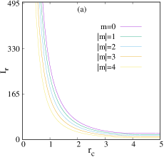
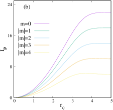
Figure 10.: Variation of $I_{\mathrm{\mathbf{r}}}$ and $I_{\mathrm{\mathbf{p}}}$ in 3DCHO, with $r_{c}$, for all allowed $|m|$ values of $1g$ state, in panels (a) and (b) respectively [130]. See text for details.

At this juncture, a few words may be devoted to the influence of $\omega$ on $I_{\mathrm{\mathbf{r}}},I_{\mathrm{\mathbf{p}}}$. In order to establish this, Fig. 11 depicts plots of $I_{\mathrm{\mathbf{r}}}$ and $I_{\mathrm{\mathbf{p}}}$ against $r_{c}$, for 5 selected $\omega^{2}$ ($1,2,4,8,32$), in bottom ((a), (b)) and top ((c), (d)) panels. These are provided for $1p$ state; left and right panels characterize $|m|=0$ and 1 respectively. Evidently at a fixed $r_{c}$, $I_{\mathrm{\mathbf{r}}}$ grows and $I_{\mathrm{\mathbf{p}}}$ decays with increment in $\omega$. At a certain $\omega$, dependence of these measures on $n_{r},l,m$ is similar to that in 3DQHO. As $\omega$ goes up, there is more localization, hence compactness in single-particle density increases with oscillation strength.

An in-depth analysis of $I$ reveals that, a gradual increase in $r_{c}$ should lead to a delocalization of the system in such a way that, at $r_{c}\rightarrow\infty$ it should approach towards an 3DQHO. On the contrary, when $r_{c}\rightarrow 0$ the impact of confinement is maximum. It suffices for us to vary $r_{c}$ from $0.1$ to $8$. This parametric increase in $r_{c}$ elicits the system from an extremely confined environment to a free 3DQHO scenario.

Table 9.: $I_{t}$ for $1p$-$1f$ $(n_{r}=0)$ orbitals at six different $r_{c}$ [130]. See text for details.

$|m|$	$r_{c}=0.1$	$r_{c}=0.5$	$r_{c}=1$	$r_{c}=2$	$r_{c}=7$	$r_{c}=\infty$
$I_{t}(1p)^{a}$
$0^{{\dagger}}$	121.01515	120.98286	120.491051	113.776614	100.00000000	100
1	57.53752	57.5166	57.1034	55.318	36.0000	36
$I_{t}(1d)^{b}$
$0^{{\dagger}}$	233.15973	233.117506	232.518248	223.80357	196.000000000	196
1	138.93098	138.89164	138.3419	130.2598	100.00000	100
2	68.870938	68.8380	68.3884	61.8358	36.00000	36
$I_{t}(1f)^{c}$
$0^{{\dagger}}$	380.432960	380.388051	379.716077	369.644758	324.0000000	324
1	255.126029	255.083860	254.452650	244.935911	196.00000	196
2	154.706834	154.669915	154.117184	145.762637	100.00000	100
3	79.1753741	79.1461919	78.7096703	72.1249096	36.00000	36

${}^{\dagger}$ These also correspond to upper bounds, given in Eq. (66).

${}^{a}$ Lower bounds Eq. (11), for $1p$ at 6 $r_{c}$ are: 10.70940, 10.71226, 10.75598,

11.39074,12.96, 12.96.

${}^{b}$ Lower bounds Eq. (11), for $1d$ at 6 $r_{c}$ are: 5.55842, 5.559428, 5.573756,

5.79079,6.61224, 6.61224.

${}^{c}$ Lower bounds Eq. (11), for $1f$ at 6 $r_{c}$ are: 3.40664, 3.40704, 3.41307,

3.506068, 4, 4.

Next, Table 11 shows evaluated $R_{\mathrm{\mathbf{r}}}^{\alpha},R_{\mathrm{\mathbf{p}}}^{\beta},R_{t}^{(\alpha,\beta)}$ for first two ($n_{r}=1,2$) $s,p$ and $d$ states of 3DCHO at a selected set of $r_{c}$ values. $R_{\mathrm{\mathbf{r}}}^{\alpha}$, starting from a $(-)$ve value at very low $r_{c}$, continuously increases, before finally reaching to the respective 3DQHO limit. This pattern in $R_{\mathrm{\mathbf{r}}}^{\alpha}$ distinctly expresses delocalization of the system with growth in $r_{c}$. In contrast, $R_{\mathrm{\mathbf{p}}}^{\beta}$, for all states generally tend to diminish monotonically with $r_{c}$, again converging to 3DQHO in the end. The analysis of $R_{t}^{(\alpha,\beta)}$ shows that, for $l=0$ states it lowers with $r_{c}$ to reach the unconfined result. However, for $1p$ state, it advances with $r_{c}$ to attain the 3DQHO limit. In case of $2p,1d$ and $2d$ states it initially increases with $r_{c}$, then passes through a maximum, and finally convenes to limiting 3DQHO result. At small $r_{c}$ (up to $\approx 2$), $n_{r}=1$ states have higher $R_{\mathrm{\mathbf{r}}}^{\alpha}$ compared to their $n_{r}=2$ counterparts. But at moderate $r_{c}$ ($>2$) region the situation alters; the $n_{r}=2$ states now possess larger $R_{\mathrm{\mathbf{r}}}^{\alpha}$. Moreover this crossover region appears at larger $r_{c}$ with rise in $l$. This observation concludes that, at smaller $r_{c}$ region the effect of confinement is more pronounced for higher $n_{r}$ states (as $n_{r}=1$ states possess higher $R_{\mathrm{\mathbf{r}}}^{\alpha}$ values than that of respective $n_{r}=2$ states). There is no such crossover in $R_{\mathrm{\mathbf{p}}}^{\beta}$ and $R_{t}^{(\alpha,\beta)}$ in any of these reported states. The above observations are graphically demonstrated in Fig. 12, where in segments (a)-(c), $R_{\mathrm{\mathbf{r}}}^{\alpha},R_{\mathrm{\mathbf{p}}}^{\beta},R_{t}^{(\alpha,\beta)}$ of first five circular states are presented as function of $r_{c}$. Panel (a) leads to the fact that, for all of them, $R_{\mathrm{\mathbf{r}}}^{\alpha}$’s quite steadily progress with $r_{c}$ and finally converge to 3DQHO. Similarly, from panel (b) it is clear that, $R_{\mathrm{\mathbf{p}}}^{\beta}$ shows reverse pattern with $r_{c}$, before reaching 3DQHO-limit. From the last panel, it appears that, for $l=0$ state, $R_{t}^{(\alpha,\beta)}$ abates with $r_{c}$, whereas an opposite trend occurs otherwise. Also one finds that major changes in $R_{t}^{(\alpha,\beta)}$ occurs in the range of $r_{c}$ varying from 2.65-5.30, with the higher state showing most predominant effect (see Figs. 15 and 17 later for $S_{t}$ and $E_{t}$, for similar effects). Some of these may not be evident from the figure as such, but becomes clear upon magnification of the plot, in consultation with the data given in Table 11.

Table 10.: $I_{\mathrm{\mathbf{r}}},I_{\mathrm{\mathbf{p}}}$ for $2p$-$2m$ ($|m|=1$) states in 3DCHO, at six selected $r_{c}$ [130].

$l$	$r_{c}=0.1$	$r_{c}=0.5$	$r_{c}=1$	$r_{c}=2$	$r_{c}=7$	$r_{c}=\infty$
$I_{\mathrm{\mathbf{r}}}$
1	19544.75146	781.7758499	195.3902144	48.61008407	14.000000000	14
2	28201.56829	1128.0488516	281.9599554	70.272141773	18.000000000	18
3	37976.00550	1519.027385	379.70865634	94.73419843	22.0000000000	22
4	48838.86407	1953.5428786	488.3419262	121.91517166	26.0000000000	26
5	60766.49285	2430.649110	607.62258270	151.75456390	30.0000000001	30
6	73739.4732	2949.5692932	737.3562778	184.204055587	34.0000000743	34
7	87741.58879	3509.6547640	877.38084537	219.22364350	38.00000037	38
8	102759.07974	4110.3551463	1027.5587357	256.77944910	42.0000017797	42
9	118780.106607	4751.196872	1187.77161130	296.84230573	46.0000074341	46
$I_{\mathrm{\mathbf{p}}}$
1	0.01221	0.3054	1.222	4.917	14.000	14
2	0.0133333	0.333337	1.33356	5.34750	18.00000	18
3	0.014439157	0.36097833	1.4438781	5.7743588	21.999997	22
4	0.0154743767	0.38685628	1.54723822	6.1782594	26.0000000	26
5	0.016426161	0.4106495	1.6423270	6.55303527	30.000000	30
6	0.017296672	0.4324115849	1.7293332625	6.898114452	34.00000	34
7	0.0180927445	0.4523131126	1.808922468	7.21517631	38.00000	38
8	0.0188222240	0.470550071	1.88186836	7.50667165	41.9999991	42
9	0.019492648	0.487310795	1.94891804	7.775182	45.99998	46

To gain further insight, Fig. 13 delineates $R^{\alpha}_{\mathrm{\mathbf{r}}},R^{\beta}_{\mathrm{\mathbf{p}}},R_{t}^{(\alpha,\beta)}$, in left (a), middle (b), right (c) panels, for lowest five circular states with changes in $n_{r}$ (maximum being 9). Four different $r_{c}$’s are chosen, namely, $0.1,3,5,\infty$ in segments (A)-(D) from bottom to top. At the lowest $r_{c}$, for all $l$, $R^{\alpha}_{\mathrm{\mathbf{r}}}$’s gradually falls off with advancement in $n_{r}$, providing highest values for $l=0$. But for non-zero $l$, it increases with $l$ for smaller $n_{r}$. However, at $n_{r}>6$, there seems to be a crossover between $l=1$ and $l=2$ states. Hence it can be concluded that, effect of confinement is maximum, minimum for $l=1$, $l=0$ states respectively. At a fixed $l$ and $r_{c}$ (lower region), higher $n_{r}$-states encounter the confinement to a greater extent. On the other hand, both $R^{\beta}_{\mathrm{\mathbf{p}}}$ (b) and $R_{t}^{(\alpha,\beta)}$ (c) show inverse trend. For smaller $n_{r}$, both these quantities follow the sequence $1g>1f>1d>1p>1s$, which however, gets reversed ($1s>1p>1d>1f>1g$) at higher $n_{r}$. These results infers that, at lower $r_{c}$ region quantum effect gets amplified as information content decreases, whereas total information increases with $n_{r}$. The first column (a) interestingly shows the appearance of maximum in $R^{\alpha}_{\mathrm{\mathbf{r}}}$ at some moderate $r_{c}$, whose positions get right shifted as $r_{c}$ enhances. Apparently there exists an interplay between two opposing effects: (i) radial confinement (localization) (ii) accumulation of nodes with $n_{r}$ (delocalization). As $r_{c}$ progresses, delocalization prevails for lower $n_{r}$. Hence with gradual relaxation in confinement, states with larger $n_{r}$ get delocalized. At $r_{c}\rightarrow\infty$, the second effect predominates; so the system behaves like 3DQHO. In second and third columns, one sees that, both $R^{\beta}_{\mathrm{\mathbf{p}}},R_{t}^{(\alpha,\beta)}$ enhance with $n_{r}$. At $r_{c}\rightarrow\infty$, these two quantities approach the respective 3DQHO-limit, as predicted.

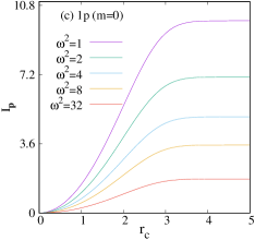
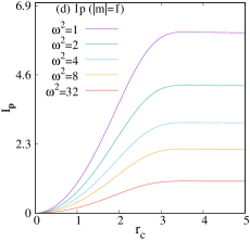
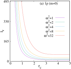
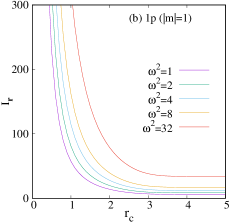
Figure 11.: Plots of $I_{\mathrm{\mathbf{r}}}$ and $I_{\mathrm{\mathbf{p}}}$ in bottom ((a), (b)) and top ((c),(d)) panels in 3DCHO with $r_{c}$, of $1p$ state at five selected $\omega^{2}(1,2,4,8,32)$. Left, right columns correspond to $|m|=0$, 1 respectively [130].

Next we move to $S$ in Table 12, where $S_{\mathrm{\mathbf{r}}},S_{\mathrm{\mathbf{p}}}$ and $S_{t}$ are demonstrated for $1s,2s,1p,2p,1d,2d$ states of 3DCHO at same set of $r_{c}$ of the previous table. Akin to $R^{\alpha}_{\mathrm{\mathbf{r}}}$, $S_{\mathrm{\mathbf{r}}}$ also yield $(-)$ve values for all six states at very low $r_{c}$, and then continuously increase until reaching the limiting 3DQHO value. This trend of $S_{\mathrm{\mathbf{r}}}$ also interprets the delocalization of 3DCHO with progress in $r_{c}$. Like $R^{\beta}_{\mathrm{\mathbf{p}}}$, $S_{\mathrm{\mathbf{p}}}$ also offers a reverse nature (continuous decrease with $r_{c}$) of $S_{\mathrm{\mathbf{r}}}$ (and $R^{\alpha}_{\mathrm{\mathbf{r}}}$); from an initial $(+)$ve value, consistently falls off to reach 3DQHO. $S_{t}$’s for both $1s,1p$ states decrease to attain 3DQHO result. Interestingly, for $1d$ state it first declines, attains a minimum value, then rises to a maximum and ultimately reaches to 3DQHO values. But for $2s,2p,2d$ states it first increases, then reaches a maximum and finally merges to borderline 3DQHO values.

Table 11.: $R_{\mathrm{\mathbf{r}}}^{\alpha},R_{\mathrm{\mathbf{p}}}^{\beta}$ and $R_{t}^{\alpha,\beta}$ for lowest three $l$ (having $n_{r}=1,2$) states in 3DCHO at eight selected values of $r_{c}$. $R_{t}^{\alpha,\beta}$ for all these states obey the lower bound given in Eq. (57) [181].

$r_{c}$	$R_{\mathrm{\mathbf{r}}}^{\alpha}$	$R_{\mathrm{\mathbf{p}}}^{\beta}$	$R_{t}^{\alpha,\beta}$	$r_{c}$	$R_{\mathrm{\mathbf{r}}}^{\alpha}$	$R_{\mathrm{\mathbf{p}}}^{\beta}$	$R_{t}^{\alpha,\beta}$
$1s$				$2s$
0.1	$-$6.0366917844	12.247171	6.210480	0.1	$-$6.0653334752	14.251561	8.186227
0.2	$-$3.9572613535	10.167740	6.210479	0.2	$-$3.9858896952	12.172113	8.186223
0.5	$-$1.2088403559	7.4192722	6.210431	0.5	$-$1.2369267194	9.422993	8.186067
1.0	0.8636306014	5.3460818	6.209712	1.0	0.8438971150	7.339578	8.183475
5.0	3.6326806767	2.5410652	6.173745	5.0	4.5764993107	2.616203	7.192702
8.0	3.6326909163	2.5410540	6.173744	8.0	4.5767695172	2.614825	7.191594
$\infty$	3.6326909163	2.5410540	6.173744	$\infty$	4.5767695172	2.614825	7.191594
$1p$				$2p$
0.1	$-$6.1671363542	12.806502	6.639365	0.1	$-$6.29011971	14.178463	7.888343
0.2	$-$4.0876997330	10.727065	6.639366	0.2	$-$4.21067738	12.099025	7.888348
0.5	$-$1.3390273792	7.978413	6.639386	0.5	$-$1.46177311	9.350298	7.888525
1.0	0.7373200936	5.902381	6.639701	1.0	0.61816051	7.273091	7.891251
5.0	3.8830108378	2.834951	6.717917	5.0	4.57588095	2.982808	7.558689
8.0	3.8830566606	2.834947	6.718004	8.0	4.57683522	2.982008	7.558843
$\infty$	3.8830566606	2.834947	6.718004	$\infty$	4.57683522	2.982008	7.558843
$1d$				$2d$
0.1	$-$6.1181191683	13.228954	7.110835	0.1	$-$6.2478841627	14.295117	8.047233
0.2	$-$4.0386800101	11.149516	7.110836	0.2	$-$4.1684423307	12.215678	8.047236
0.5	$-$1.2899046230	8.400780	7.110875	0.5	$-$1.4195583633	9.466934	8.047376
1.0	0.7880364400	6.323450	7.111487	1.0	0.6600654534	7.389472	8.049538
5.0	4.2284239258	3.048859	7.277282	5.0	4.8017869530	3.233068	8.034855
8.0	4.2285908429	3.047026	7.275616	8.0	4.8046032500	3.230664	8.035267
$\infty$	4.2285908429	3.047026	7.275616	$\infty$	4.8046032500	3.230664	8.035267

Figure 14 delineates behavioral trends of $S_{\mathrm{\mathbf{r}}}$, $S_{\mathrm{\mathbf{p}}}$, $S_{t}$ with $r_{c}$, in segments (a)-(c), for same five states of Fig. 12 (done for $R$). One notices that, both Figs. 12 and 14 offer qualitatively analogous changes with respect to $r_{c}$ variation; thus signalling comparable trends in $R$ and $S$. For all these states $S_{\mathrm{\mathbf{r}}}$’s tend to progress with $r_{c}$ and then reach the corresponding $r$-space 3DQHO, while $S_{\mathrm{\mathbf{p}}}$’s reduce before attaining that. The last panel portrays that, for $1s,1p$ states $S_{t}$ decreases with $r_{c}$, while for the remaining three states, $S_{t}$ passes through a minimum. It is worth noting that, in the $1p$ state, $R_{t}$ progresses and $S_{t}$ regresses after $r_{c}=2.65$. In both occasions, however, as usual they all gain the limiting 3DQHO behavior at a sufficiently large $r_{c}$.

In Fig. 15, $S_{\mathrm{\mathbf{r}}}$ (a), $S_{\mathrm{\mathbf{p}}}$ (b), $S_{t}$ (c) of $l=0-4$ states are plotted with respect to $n_{r}$ at same four values of $r_{c}$ in Fig. 13, in panels marked with (A)-(D) from bottom to top. Again, these graphs produce resembling shape and propensity as in Fig. 13. Thus in harmony with $R^{\alpha}_{\mathrm{\mathbf{r}}}$ (for all five $l$ at the lowest $r_{c}=0.1$), $S_{\mathrm{\mathbf{r}}}$ gets lowered in A(a), while $S_{\mathrm{\mathbf{p}}}$s and $S_{t}$s accelerate with $n_{r}$ in A(b) and A(c), respectively. This supports our previous observation (of $R$ in Fig. 13) that, at very low $r_{c}$, the effect of confinement is more prominent in high-lying states, signifying an intensification of quantum nature in such a scenario. As usual, like $R^{\alpha}_{\mathrm{\mathbf{r}}}$ here also, the first column (a) shows the appearance of maximum in $S_{\mathrm{\mathbf{r}}}$ plot with gradual progress of $r_{c}$ from the bottom to top. Their positions switch to right as $r_{c}$ enhances. This observation indicates that, at $r_{c}\rightarrow\infty$ the system behaves like 3DQHO.

At this point we proceed for the last measure ($E$) of this study in Table 13. A cross-section of $E_{\mathrm{\mathbf{r}}},E_{\mathrm{\mathbf{p}}},E_{t}$ for $1s,2s,1p,2p,1d,2d$ states of 3DCHO (same set of $r_{c}$ as used in previous table) is offered. One notices that, $E_{\mathrm{\mathbf{r}}}$ reduces (as opposed to $R^{\alpha}_{\mathrm{\mathbf{r}}},S_{\mathrm{\mathbf{r}}}$) while $E_{\mathrm{\mathbf{p}}}$ progresses (in contrast to $R^{\beta}_{\mathrm{\mathbf{p}}},S_{\mathrm{\mathbf{p}}}$) with rise in $r_{c}$. However, the nature of variation of $E_{t}$ with $r_{c}$ varies from state to state. For $1s,1p,1d$ states, it enhances with $r_{c}$, while $2s,2p,2d$ states, it goes through a minimum. These changes in $E_{\mathrm{\mathbf{r}}},E_{\mathrm{\mathbf{p}}}$ and $E_{t}$ with $r_{c}$ are demonstrated pictorially in Fig. 16, in left (a), middle (b) and right (c) panels for first five node-less states. It is found that, $E_{t}$ for $1s,1p,1d$ states advances with $r_{c}$, while for $1f,1g$ states it decreases. Interestingly, at large $r_{c}$, both $E_{\mathrm{\mathbf{r}}},E_{\mathrm{\mathbf{p}}}$ decline with growth in $l$. Finally, Fig. 17, depicts $E_{\mathrm{\mathbf{r}}},E_{\mathrm{\mathbf{p}}},E_{t}$ (in columns (a),(b),(c)) for $l=0-4$ states as functions of $n_{r}$ at four different $r_{c}$ (in segments A-D). At the lowest $r_{c}$ considered, $E_{\mathrm{\mathbf{r}}}$ advances with $n_{r}$. However, the first column (a) suggests that, a minimum appears in $E_{\mathrm{\mathbf{r}}}$ graphs as $r_{c}$ is increased. Also the positions of these minima shift towards right with rise in $r_{c}$. On the contrary, for all concerned $r_{c}$, both $E_{\mathrm{\mathbf{p}}}$, $E_{t}$ decay with $n_{r}$.

All the discussed measures of Eq. (72) have been investigated with change of $r_{c}$, choosing two different and widely used values of $b$ ($1,\frac{2}{3}$). Note that, for $b=1$, $C_{ES}^{(2)}$ transforms to $C_{LMC}$; similarly $C_{IS}^{(1)}$ coincides with $C_{IS}$ at $b=\frac{2}{3}$. In order to simplify the discussion, a few words may be devoted to the notation used. A uniform symbol $C_{order_{s},disorder_{s}}^{b}$ is used; where the two subscripts refer to two order ($E,I$) and disorder ($S,R$) parameters. Another subscript $s$ is used to specify the space; viz., $r,p$ or $t$ (total). Two scaling parameters $b=\frac{2}{3},1$ are identified with superscripts (1), (2). These measures are examined systematically for $1s,~{}1p,~{}1d,~{}2s,~{}1f,~{}2p,~{}1g$ and $2d$ states in conjugate spaces. In this part we will discuss the outcome extracted from a recent complexity analysis undertaken by us. The detailed results with relevant figures and tables will be published elsewhere separately.

Now we lay our focus on $C_{E_{\mathrm{\mathbf{r}}}S_{\mathrm{\mathbf{r}}}}^{(1)},C_{E_{\mathrm{\mathbf{p}}}S_{\mathrm{\mathbf{p}}}}^{(1)}$ and $C_{E_{\mathrm{\mathbf{r}}}S_{\mathrm{\mathbf{r}}}}^{(2)},C_{E_{\mathrm{\mathbf{p}}}S_{\mathrm{\mathbf{p}}}}^{(2)}$ respectively. $C_{E_{\mathrm{\mathbf{r}}}S_{\mathrm{\mathbf{r}}}}^{(1)}$ decreases and $C_{E_{\mathrm{\mathbf{p}}}S_{\mathrm{\mathbf{p}}}}^{(1)}$ increases with rise of $r_{c}$, before reaching the borderline 3DQHO result. As mentioned earlier, the 3DCHO model acts as an intermediate between the PISB and 3DQHO [130]. That means, an enhancement in $r_{c}$ should lead the system towards delocalization (equilibrium), which is supported by the declining nature of $C_{E_{\mathrm{\mathbf{r}}}S_{\mathrm{\mathbf{r}}}}^{(1)}$ with progress in $r_{c}$. At a fixed $l$, $C_{E_{\mathrm{\mathbf{r}}}S_{\mathrm{\mathbf{r}}}}^{(1)}$ progresses with $n_{r}$. It may be noted that in a 3DCHO, number of nodes varies with $n_{r}$ only (in contrast to, say the H atom, where it depends on both $n=n_{r}$ and $l$). Hence in this case, the increment in number of nodes takes the system towards the side of ordering. But no such pattern is observed for $C_{E_{\mathrm{\mathbf{p}}}S_{\mathrm{\mathbf{p}}}}^{(1)}$. The variation of $C_{E_{\mathrm{\mathbf{r}}}S_{\mathrm{\mathbf{r}}}}^{(2)},~{}C_{E_{\mathrm{\mathbf{p}}}S_{\mathrm{\mathbf{p}}}}^{(2)}$ with change of $r_{c}$ reveals that, former advances with growth of $r_{c}$ indicating that this is more inclined towards order. On the other hand, at first $C_{E_{\mathrm{\mathbf{p}}}S_{\mathrm{\mathbf{p}}}}^{(2)}$ decreases with $r_{c}$, attains a minimum and finally merges to 3DQHO. The ordering of $C_{E_{\mathrm{\mathbf{r}}}S_{\mathrm{\mathbf{r}}}}^{(2)}$ regarding $n_{r}$ quantum number is akin to $C_{E_{\mathrm{\mathbf{r}}}S_{\mathrm{\mathbf{r}}}}^{(1)}$. This observation complements our previous conjecture that, an increase in number of nodes takes the system towards disequilibrium. It is noticed that, after a certain $r_{c}$ ($\approx 3$), both $C_{E_{\mathrm{\mathbf{r}}}S_{\mathrm{\mathbf{r}}}}^{(2)},C_{E_{\mathrm{\mathbf{p}}}S_{\mathrm{\mathbf{p}}}}^{(2)}$ show analogous nature (increase to reach their respective limiting value). Here, exploring these two sets of complexity measure, namely, $C^{(1)}_{ES}$ and $C^{(2)}_{ES}$, it is evident that, $C_{E_{\mathrm{\mathbf{r}}}S_{\mathrm{\mathbf{r}}}}^{(1)}$ and $C_{E_{\mathrm{\mathbf{p}}}S_{\mathrm{\mathbf{p}}}}^{(1)}$ complement each other better (as former decreases, later increases with $r_{c}$) and more tends towards disorder (equilibrium), whereas the other set is inclined towards the order-direction. Thus, $C_{ES}^{(1)}$ with $b=\frac{2}{3}$ explains the system better. It is important to point out that, when 3DCHO approaches to 3DQHO, $C_{E_{\mathrm{\mathbf{r}}}S_{\mathrm{\mathbf{r}}}}^{(1)}$ becomes equal to $C_{E_{\mathrm{\mathbf{p}}}S_{\mathrm{\mathbf{p}}}}^{(1)}$.

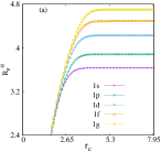
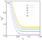
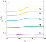
Figure 12.: Plots of $R_{\mathrm{\mathbf{r}}}^{\alpha}$, $R_{\mathrm{\mathbf{p}}}^{\beta}$, $R_{t}^{(\alpha,\beta)}$ against $r_{c}$ for first five circular states of 3DCHO in panels (a), (b), (c) respectively [181]. See text for details.

In the same direction, now we interpret the pattern changes of $C_{E_{\mathrm{\mathbf{r}}}R_{\mathrm{\mathbf{r}}}}^{(1)},C_{E_{\mathrm{\mathbf{p}}}R_{\mathrm{\mathbf{p}}}}^{(1)}$ with $r_{c}$. At first, $C_{E_{\mathrm{\mathbf{r}}}R_{\mathrm{\mathbf{r}}}}^{(1)}$ declines with growth of $r_{c}$, then passes through a minimum and finally converges to respective 3DQHO result. This minimum gets flatter with rise of both $n_{r},~{}l$. Here also $C_{E_{\mathrm{\mathbf{r}}}R_{\mathrm{\mathbf{r}}}}^{(1)}$ shows similar trend as observed in $C_{E_{\mathrm{\mathbf{r}}}S_{\mathrm{\mathbf{r}}}}^{(1)}$, viz., (i) like $C_{E_{\mathrm{\mathbf{r}}}S_{\mathrm{\mathbf{r}}}}^{(1)}$, $C_{E_{\mathrm{\mathbf{r}}}R_{\mathrm{\mathbf{r}}}}^{(1)}$ is more aligned towards disorder (ii) at a particular $l$, they progress with $n_{r}$. The first point suggests that, like $C_{E_{\mathrm{\mathbf{r}}}S_{\mathrm{\mathbf{r}}}}^{(1)}$, $C_{E_{\mathrm{\mathbf{r}}}R_{\mathrm{\mathbf{r}}}}^{(1)}$ also interprets that, with increase in $r_{c}$ the system progresses towards 3DQHO from PISB via 3DCHO. The second point says that, an increase/decrease in number of nodes leads towards the direction of order/disorder respectively. Like $C_{E_{\mathrm{\mathbf{p}}}S_{\mathrm{\mathbf{p}}}}^{(1)}$, $C_{E_{\mathrm{\mathbf{p}}}R_{\mathrm{\mathbf{p}}}}^{(1)}$ increases with growth in $r_{c}$. Moreover, at a definite $l$, $C_{E_{\mathrm{\mathbf{p}}}R_{\mathrm{\mathbf{p}}}}^{(1)}$ falls off with $n_{r}$. At smaller $r_{c}$ region ($\approx 3$), both $C_{E_{\mathrm{\mathbf{r}}}R_{\mathrm{\mathbf{r}}}}^{(2)},C_{E_{\mathrm{\mathbf{p}}}R_{\mathrm{\mathbf{p}}}}^{(2)}$ vary slowly. At around same $r_{c}$, the former jumps and latter drops to attain the borderline 3DQHO limit. For both $C_{E_{\mathrm{\mathbf{r}}}R_{\mathrm{\mathbf{r}}}}^{(2)}$ and $C_{E_{\mathrm{\mathbf{p}}}R_{\mathrm{\mathbf{p}}}}^{(2)}$ absolute values of the slope of the curve enhance as $n_{r}$ grows (fixed $l$) and decrease with growth of $l$ (fixed $n_{r}$). The dependence of $C_{E_{\mathrm{\mathbf{r}}}R_{\mathrm{\mathbf{r}}}}^{(2)}$ on $n_{r}$ is similar to $C_{E_{\mathrm{\mathbf{r}}}R_{\mathrm{\mathbf{r}}}}^{(1)}$. This again validates the dependency of this complexity measure on number of nodes of the system. Once again one may conclude that, out of $C^{(1)}_{ER}$ and $C^{(2)}_{ER}$, the former offers a more complete knowledge about the characteristics of 3DCHO. Apart from that, $C_{E_{\mathrm{\mathbf{p}}}R_{\mathrm{\mathbf{p}}}}^{(1)}$ shows more lucid trend than $C_{E_{\mathrm{\mathbf{p}}}S_{\mathrm{\mathbf{p}}}}^{(1)}$ with respect to dependence of quantum number $n_{r}$. Hence, in practice, $C^{(1)}_{ER}$ may possibly be considered a better measure of complexity than $C^{(1)}_{ES}$.

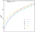
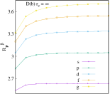
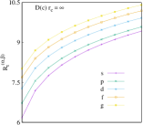
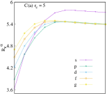
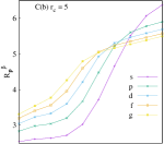
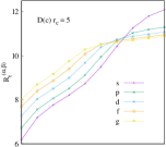
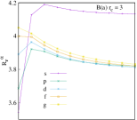
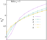
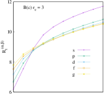
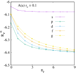
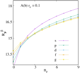
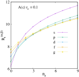
Figure 13.: Plot of $R^{\alpha}_{\mathrm{\mathbf{r}}}$ (a), $R^{\beta}_{\mathrm{\mathbf{p}}}$ (b) and $R_{t}^{(\alpha,\beta)}$ (c) versus $n_{r}$ (at $\omega=1$) for $s,p,d,f,g$ states at four particular $r_{c}$’s of 3DCHO, namely, $0.1,3,5,\infty$ in panels (A)-(D). $R_{t}^{(\alpha,\beta)}$’s for all these states obey the lower bound given in Eq. (57) [181]. For more details, consult text.

Now we discuss variations of $\{C_{I_{\mathrm{\mathbf{r}}}S_{\mathrm{\mathbf{r}}}}^{(1)},C_{I_{\mathrm{\mathbf{p}}}S_{\mathrm{\mathbf{p}}}}^{(1)}\}$ and $\{C_{I_{\mathrm{\mathbf{r}}}S_{\mathrm{\mathbf{r}}}}^{(2)},C_{I_{\mathrm{\mathbf{p}}}S_{\mathrm{\mathbf{p}}}}^{(2)}\}$ with changes in $r_{c}$ for all the states mentioned above. Interestingly. in this occasion, the nature of alteration of $\{C_{I_{\mathrm{\mathbf{r}}}S_{\mathrm{\mathbf{r}}}}^{(1)},C_{I_{\mathrm{\mathbf{p}}}S_{\mathrm{\mathbf{p}}}}^{(1)}\}$ with $r_{c}$ varies from state to state. At a fixed $n_{r}$, both $C_{I_{\mathrm{\mathbf{r}}}S_{\mathrm{\mathbf{r}}}}^{(1)},C_{I_{\mathrm{\mathbf{p}}}S_{\mathrm{\mathbf{p}}}}^{(1)}$ increase with $l$. Further, at a fixed $l$, they elevate with growth in $n_{r}$. This behavior of $C_{I_{\mathrm{\mathbf{r}}}S_{\mathrm{\mathbf{r}}}}^{(1)}$ with $n_{r}$, is again connected to the nodal structure in $C_{ES}$ and $C_{ER}$. On the contrary, $C_{I_{\mathrm{\mathbf{r}}}S_{\mathrm{\mathbf{r}}}}^{(2)}$, $C_{I_{\mathrm{\mathbf{p}}}S_{\mathrm{\mathbf{p}}}}^{(2)}$ increase and decrease with growth in $r_{c}$ and finally approach to respective 3DQHO. This obviously conveys that, $C_{I_{\mathrm{\mathbf{r}}}S_{\mathrm{\mathbf{r}}}}^{(2)}$ is a descriptor of disequilibrium. At a particular $n_{r}$ both $C_{I_{\mathrm{\mathbf{r}}}S_{\mathrm{\mathbf{r}}}}^{(2)}$, $C_{I_{\mathrm{\mathbf{p}}}S_{\mathrm{\mathbf{p}}}}^{(2)}$ enhance with advancement in $l$. Also, at a certain $l$, they enhance with improvement of $n_{r}$. However, this pattern is in agreement with $C_{ES}$ and $C_{ER}$. In case of 3DCHO, both $\{C_{I_{\mathrm{\mathbf{r}}}S_{\mathrm{\mathbf{r}}}}^{(1)},~{}C_{I_{\mathrm{\mathbf{p}}}S_{\mathrm{\mathbf{p}}}}^{(1)}\}$ and $\{C_{I_{\mathrm{\mathbf{r}}}S_{\mathrm{\mathbf{r}}}}^{(2)},C_{I_{\mathrm{\mathbf{p}}}S_{\mathrm{\mathbf{p}}}}^{(2)}\}$ are unable to explain the delocalization of the system from PISB to 3DQHO through the increase in $r_{c}$.

Table 12.: $S_{\mathrm{\mathbf{r}}},S_{\mathrm{\mathbf{p}}}$ and $S_{t}$ for lowest three $l$ (having $n_{r}=1,2$) states in 3DCHO at eight selected values of $r_{c}$. $S_{t}$ for all these states obey the lower bound given in Eq. (53) [181].

$r_{c}$	$S_{\mathrm{\mathbf{r}}}$	$S_{\mathrm{\mathbf{p}}}$	$S_{t}$	$r_{c}$	$S_{\mathrm{\mathbf{r}}}$	$S_{\mathrm{\mathbf{p}}}$	$S_{t}$
$1s$				$2s$
0.1	$-$6.232173222	12.8494	6.6172	0.1	$-$6.4460987687	14.6389	8.1928
0.2	$-$4.152747179	10.7700	6.6172	0.2	$-$4.3666534417	12.5595	8.1928
0.5	$-$1.404504328	8.0214	6.6168	0.5	$-$1.6176276192	9.8106	8.1929
1.0	0.6652222004	5.9458	6.6110	1.0	0.4641636149	7.731	8.195
5.0	3.2170947394	3.217094	6.434189	5.0	4.150729546	4.1510	8.3017
8.0	3.2170948239	3.217094	6.434189	8.0	4.150745547	4.15074	8.30148
$\infty$	3.2170948239	3.217094	6.434189	$\infty$	4.150745547	4.15074	8.30148
$1p$				$2p$
0.1	$-$6.38738206	13.418	7.030	0.1	$-$6.651966568	14.7283	8.0763
0.2	$-$4.30794705	11.338	7.030	0.2	$-$4.572523919	12.6489	8.0763
0.5	$-$1.55934019	8.5894	7.0300	0.5	$-$1.823606736	9.9000	8.0763
1.0	0.51599338	6.5114	7.0273	1.0	0.256528223	7.82132	8.07784
5.0	3.4874566574	3.4875	6.9750	5.0	4.1477548396	4.1483	8.2960
8.0	3.4874576660	3.487457	6.974915	8.0	4.14786196159	4.147861	8.295723
$\infty$	3.4874576660	3.487457	6.974915	$\infty$	4.14786196159	4.147861	8.295723
$1d$				$2d$
0.1	$-$6.3553068427	14.0035	7.6481	0.1	$-$6.5939939435	15.0676	8.4736
0.2	$-$4.2758683878	11.9241	7.6481	0.2	$-$4.5145520348	12.9881	8.4736
0.5	$-$1.52712156	9.1753	7.6481	0.5	$-$1.7656649279	10.2393	8.4736
1.0	0.5503764295	7.0964	7.6467	1.0	0.3140078818	8.1605	8.4745
5.0	3.8426303929	3.8427	7.6853	5.0	4.3885945973	4.3909	8.7794
8.0	3.8426381378	3.842638	7.685276	8.0	4.389113529281	4.389113	8.778227
$\infty$	3.8426381378	3.842638	7.685276	$\infty$	4.389113529281	4.389113	8.778227

Finally, we mention a few words regarding the behavioral pattern in our last complexity measure, viz., $C_{I_{\mathrm{\mathbf{r}}}R_{\mathrm{\mathbf{r}}}}^{(1)},C_{I_{\mathrm{\mathbf{p}}}R_{\mathrm{\mathbf{p}}}}^{(1)}$, $C_{I_{\mathrm{\mathbf{r}}}R_{\mathrm{\mathbf{r}}}}^{(2)},C_{I_{\mathrm{\mathbf{p}}}R_{\mathrm{\mathbf{p}}}}^{(2)}$, with alterations in $r_{c}$. It is found that, $C_{I_{\mathrm{\mathbf{r}}}R_{\mathrm{\mathbf{r}}}}^{(1)}$ progresses slowly with $r_{c}$ to reach respective 3DQHO values, implying that, $C_{I_{\mathrm{\mathbf{r}}}R_{\mathrm{\mathbf{r}}}}^{(1)}$ is an order parameter. At a suitable $n_{r}$, this quantity advances with $l$. In a parallel way, at constant $l$, $C_{I_{\mathrm{\mathbf{r}}}R_{\mathrm{\mathbf{r}}}}^{(1)}$ accumulates with $n_{r}$. This again means that with increase in number of nodes, the system moves towards order. Besides this, it can be concluded that, for node-less (like $1s,1p,1d,1f,1g$) states, $C_{I_{\mathrm{\mathbf{p}}}R_{\mathrm{\mathbf{p}}}}^{(1)}$ diminishes with progression in $r_{c}$. But for states having one radial node (such as $2s,2p,2d$), there appears a maximum in $C_{I_{\mathrm{\mathbf{p}}}R_{\mathrm{\mathbf{p}}}}^{(1)}$, which gets right shifted with increase in $l$. It can be said that, $C_{I_{\mathrm{\mathbf{r}}}R_{\mathrm{\mathbf{r}}}}^{(2)},C_{I_{\mathrm{\mathbf{p}}}R_{\mathrm{\mathbf{p}}}}^{(2)}$, accelerate and decelerate respectively with growth in $r_{c}$. Hence, $C^{(2)}_{IR}$ is an indicator of order. Like $C^{(1)}_{IR}$, both $C_{I_{\mathrm{\mathbf{r}}}R_{\mathrm{\mathbf{r}}}}^{(2)}$, $~{}C_{I_{\mathrm{\mathbf{p}}}R_{\mathrm{\mathbf{p}}}}^{(2)}$ enhance with emergence of $n_{r}$ and $l$ quantum numbers. A closer investigation conveys that, neither $C^{(1)}_{IR}$ nor $C^{(2)}_{IR}$ can explain the transformation of system from PISB to 3DQHO via 3DCHO. It is hoped that, this study would be useful for future references and would inspires further work along this direction.

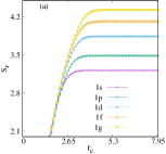
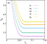
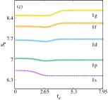
Figure 14.: Plots of $S_{\mathrm{\mathbf{r}}}$, $S_{\mathrm{\mathbf{p}}}$, $S_{t}$ against $r_{c}$ for first five circular states of 3DCHO in panels (a), (b), (c) respectively [181]. See text for details.

4.3. Relative Information

4.3.1. 1D Quantum harmonic oscillator (1DQHO)

At first we would like to explore IR in model 1DQHO in $x,p$ spaces. The underlying potential is characterized by the expression: $v(x)=\frac{1}{2}\omega^{2}x^{2}$ (mass $m$ is set to unity throughout), where $\omega$ signifies angular frequency. The normalized $x$-space wave function is expressed as ($H_{n}(x)$ refers to Hermite polynomial),

$$\psi_{n}(x)=\left(\frac{\omega}{\sqrt{2}\pi}\right)^{\frac{1}{4}}\frac{1}{\sqrt{2^{n}n!}}\ H_{n}\left(\frac{\sqrt{\omega}}{2^{\frac{1}{4}}}x\right)e^{-\frac{\omega}{2\sqrt{2}}x^{2}}.$$ (80)

Choosing $n=0$ as reference, $\frac{\sqrt{\omega}}{2^{\frac{1}{4}}}x=y$, and using definition of IR in Eq. (73), one gets,

$$\mathrm{IR}_{x}=\frac{\omega}{\sqrt{2}}\ \frac{1}{2^{n-1}n!}\int_{0}^{\infty}\ H_{n}^{2}(y)\ e^{-y^{2}}\left[\frac{\psi^{\prime}_{n}(y)}{\psi_{n}(y)}-\frac{\psi^{\prime}_{0}(y)}{\psi_{0}(y)}\right]^{2}\mathrm{d}y.$$ (81)

Here the suffix “x” denotes a position-space quantity. Now use of recurrence relation $H_{n}^{\prime}(y)=2nH_{n-1}(y)$, in conjunction with orthonormality condition of Hermite polynomial, $\int_{0}^{\infty}e^{-y^{2}}H_{m}(y)H_{k}(y)\mathrm{d}y=2^{m-1}m!\sqrt{\pi}\delta_{mk}$ ($\delta_{mn}=1$ when $m=k$, and $0$ otherwise) produces,

$$\mathrm{IR}_{x}=4n^{2}\frac{\omega}{\sqrt{2}}\ \frac{1}{2^{n-1}n!}\int_{0}^{\infty}\left[H_{n-1}(y)\right]^{2}e^{-y^{2}}\mathrm{d}y=4\sqrt{2}\ \omega n.$$ (82)

Thus Eq. (82) suggests that, IR${}_{x}$ in $n$th state may be obtained from a knowledge of $(n-1)$th-state wave function. Clearly, it increases linearly with state index $n$, with a positive slope of $4\sqrt{2}\omega$. This is in agreement with the fact that in this system, localization as well as fluctuation enhance with $\omega$. So IR${}_{x}$ result simply complements this.

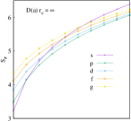
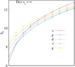
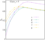
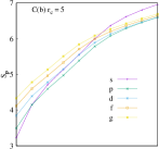
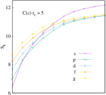
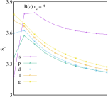
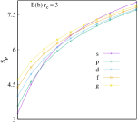
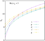
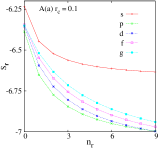
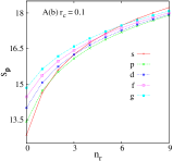
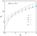
Figure 15.: Plot of $S_{\mathrm{\mathbf{r}}}$ (a), $S_{\mathrm{\mathbf{p}}}$ (b) and $S_{t}$ (c) versus $n_{r}$ (at $\omega=1$) for $s,p,d,f,g$ states at four particular $r_{c}$’s of 3DCHO, namely, $0.1,3,5,\infty$ in panels (A)-(D). $S_{t}$’s for all these states obey the lower bound given in Eq. (53) [181]. For more details, consult text.

Now we move on to $p$ space, where the normalized wave function is in the form of,

$$\psi_{n}(p)=\left(\frac{\sqrt{2}}{\omega\pi}\right)^{\frac{1}{4}}\frac{1}{\sqrt{2^{n}n!}}\ H_{n}\left(\frac{2^{\frac{1}{4}}}{\sqrt{\omega}}p\right)\ e^{-\frac{1}{\sqrt{2}\omega}\ p^{2}}.$$ (83)

Again, considering $n=0$ state as reference, setting $\frac{2^{\frac{1}{4}}}{\sqrt{\omega}}p=g$, using the recurrence relation $H_{n}^{\prime}(g)=2nH_{n-1}(g)$ and invoking orthonormality condition of Hermite polynomial, one can derive the following expression for IR${}_{p}$ after some straightforward algebra ($p$ subscript indicates $p$-space quantity), namely,

$$\mathrm{IR}_{p}=4n^{2}\sqrt{\frac{2}{\pi}}\ \frac{1}{2^{n}n!}\frac{1}{\omega}\int_{0}^{\infty}[H_{n-1}(g)]^{2}e^{-g^{2}}\mathrm{d}g=\frac{8\sqrt{2}}{\omega}\ n.$$ (84)

Thus, similar to IR${}_{x}$, here also IR${}_{p}$ of a particular oscillator state can be recovered from the wave function of adjacent lower state. Equation (84) tells that, progress of IR${}_{p}$ with $n$ is again linear like its $x$-space counterpart, slope of the straight line in this case being $\frac{8\sqrt{2}}{\omega}$. It is inversely proportional to $\omega$ in accordance with the fact that, with increase in oscillation, localization as well as fluctuation predominates. At the special value of $\omega=\sqrt{2}$, IR${}_{x}$, IR${}_{p}$ become equal ($8n$). Apart from that, like the total energy difference in a 1DQHO, $\Delta\mathrm{E_{n}}(=\mathrm{E_{n+1}}-\mathrm{E_{n}})$, the difference of IR between two successive states also remains constant, i.e., $\Delta(\mathrm{IR}_{x})=\mathrm{IR}_{x}(n+1)-\mathrm{IR}_{x}(n)=4\sqrt{2}\omega$, and $\Delta(\mathrm{IR}_{p})=\mathrm{IR}_{p}(n+1)-\mathrm{IR}_{p}(n)=\frac{8\sqrt{2}}{\omega}$.

Table 13.: $E_{\mathrm{\mathbf{r}}},E_{\mathrm{\mathbf{p}}},E_{t}$ for $1s,2s,1p,2p,1d,2d$ states in 3DCHO at eight selected $r_{c}$ [181].

$r_{c}$	$E_{\mathrm{\mathbf{r}}}$	$E_{\mathrm{\mathbf{p}}}$	$E_{t}$	$r_{c}$	$E_{\mathrm{\mathbf{r}}}$	$E_{\mathrm{\mathbf{p}}}$	$E_{t}$
$1s$				$2s$
0.1	672.0719164	0.00000398	0.0026791	0.1	1453.1909702895	0.00000057	0.00082825
0.2	84.01080088	0.00003189	0.0026791	0.2	181.6485572148	0.00000455	0.00082825
0.5	5.3814002356	0.00049808	0.00268041	0.5	11.6246913489	0.00007124	0.00082821
1.0	0.6818097823	0.00396012	0.00270005	1.0	1.4515093698	0.00057014	0.00082757
5.0	0.0634936361	0.06349340	0.00403142	5.0	0.0406758398	0.04064829	0.00165340
8.0	0.0634936347	0.06349363	0.00403144	8.0	0.040675749	0.04067560	0.00165430
$\infty$	0.0634936347	0.06349363	0.00403144	$\infty$	0.0406756097	0.04067560	0.00165450
$1p$				$2p$
0.1	803.22700816	0.00000227	0.00182938	0.1	1454.974575234	0.00000058	0.00085788
0.2	100.40423515	0.00001822	0.00182940	0.2	181.871793182	0.00000471	0.00085788
0.5	6.4281046025	0.00028463	0.00182965	0.5	11.6397197874	0.00007369	0.00085777
1.0	0.8078468658	0.00226961	0.00183350	1.0	1.454810759	0.00058839	0.00085600
5.0	0.0476202385	0.04761162	0.00226727	5.0	0.0324128865	0.03237583	0.00104939
8.0	0.047620224	0.04762022	0.00226768	8.0	0.032411515	0.03241151	0.00105050
$\infty$	0.047620224	0.04762022	0.00226768	$\infty$	0.032411515	0.03241151	0.00105050
$1d$				$2d$
0.1	851.25726418	0.00000137	0.00117301	0.1	1368.86082394	0.00000047	0.00064967
0.2	106.40757650	0.00001102	0.00117301	0.2	171.107627763	0.00000379	0.00064967
0.5	6.8111728555	0.00017222	0.00117305	0.5	10.9509523492	0.00005931	0.00064960
1.0	0.8535077417	0.00137508	0.00117364	1.0	1.3689869817	0.00047372	0.00064852
5.0	0.0357152613	0.03571436	0.00127554	5.0	0.0249812774	0.02492595	0.00062268
8.0	0.0357151695	0.03571516	0.00127557	8.0	0.0249755634	0.02497556	0.00062377
$\infty$	0.0357151695	0.03571516	0.00127557	$\infty$	0.0249755634	0.02497556	0.00062377

4.3.2. Isotropic 3D quantum harmonic oscillator (3DQHO)

We start from the normalized $r$-space wave function given as,

$$\psi_{n_{r},l}(r)=\sqrt{\frac{2\ \omega^{l+\frac{3}{2}}\ n_{r}!}{\Gamma(n_{r}+l+\frac{3}{2})}}\ \ r^{l}\ e^{-\frac{\omega r^{2}}{2}}\ L_{n_{r}}^{l+\frac{1}{2}}(\omega r^{2}).$$ (85)

In the above, $L_{n}^{\alpha}(x)$ represents the associated Laguerre polynomial. Now, using Eq. (85) and substituting $\omega r^{2}=u$, first part of Eq. (76) yields,

$$\mathrm{IR}_{\mathrm{\mathbf{r}}}=\frac{16\ \omega\ n_{r}!}{\Gamma(n_{r}+l+\frac{3}{2})}\int_{0}^{\infty}u^{l+\frac{3}{2}}e^{-u}\left[L_{n_{r}}^{l+\frac{1}{2}}(u)\right]^{2}\left(\frac{\psi_{n_{r},l}^{\prime}(u)}{\psi_{n_{r},l}(u)}-\frac{\psi_{n_{r_{1}},l}^{\prime}(u)}{\psi_{n_{r_{1}},l}(u)}\right)^{2}\mathrm{d}u.$$ (86)

Now, using the recurrence relation $\ \frac{d}{du}L_{n_{r}}^{l+\frac{1}{2}}(u)=-L_{n_{r}-1}^{l+\frac{3}{2}}(u)$, the ratios of wave functions given in the parentheses may be simplified as,

$$\frac{\psi_{n_{r},l}^{\prime}(u)}{\psi_{n_{r},l}(u)}=\frac{l}{2u}-\frac{1}{2}-\frac{L_{n_{r}-1}^{l+\frac{3}{2}}(u)}{L_{n_{r}}^{l+\frac{1}{2}}(u)},$$ (87)

the right-hand side of which, for a node-less state becomes $\left(\frac{l}{2u}-\frac{1}{2}\right)$, because the ratio of polynomials vanishes. Next one may invoke the usual orthonormality relation,

$$\int_{0}^{\infty}u^{k}e^{-u}L_{i}^{k}(u)L_{j}^{k}(u)\mathrm{d}u=\frac{(i+k)!}{i!}\ \delta_{ij}.$$ (88)

to obtain the final form of IR${}_{\mathrm{\mathbf{r}}}$ as below,

$$\mathrm{IR}_{\mathrm{\mathbf{r}}}=\frac{16\ \omega\ n_{r}!}{\Gamma(n_{r}+l+\frac{3}{2})}\ \int_{0}^{\infty}u^{l+\frac{3}{2}}e^{-u}\left[L_{n_{r}-1}^{l+\frac{3}{2}}\right]^{2}\mathrm{d}u=16\omega\ n_{r}=8\omega(n-l).$$ (89)

Equation (89) predicts that, IR${}_{\mathrm{\mathbf{r}}}$ in a 3DQHO, like its 1D counterpart, is also a linear function of $n$; however in this occasion the slope is $8\omega$ and intercept is negative. For a fixed $l$, the slope progresses and intercept decreases with $\omega$ respectively. Further, at a certain $\omega$, the intercept declines with rise of $l$. In this scenario, the particle gets more and more localized with progress of $\omega$. The relative fluctuation with respect to reference state advances with $\omega$. Dependence of IR${}_{\mathrm{\mathbf{r}}}$ on $\omega$ is reminiscent to that of $r$-space Fisher information, I${}_{\mathrm{\mathbf{r}}}$ [128]—both quantities escalate with $\omega$.

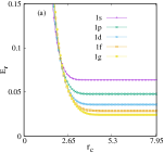
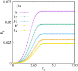
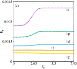
Figure 16.: Plots of $E_{\mathrm{\mathbf{r}}}$, $E_{\mathrm{\mathbf{p}}}$, $E_{t}$ against $r_{c}$ for first five circular states of 3DCHO in panels (a), (b), (c) respectively [181]. See text for details.

Analogously, in $p$-space the normalized wave function can be expressed as [182],

$$\psi_{n_{r},l}(p)=\sqrt{\frac{2\ n_{r}!}{\Gamma(n_{r}+l+\frac{3}{2})\ \ \omega^{l+\frac{3}{2}}}}\ \ p^{l}\ e^{-\frac{p^{2}}{2\omega}}\ L_{n_{r}}^{l+\frac{1}{2}}\left(\frac{p^{2}}{\omega}\right).$$ (90)

Substituting $\frac{p^{2}}{\omega}=\chi$, and going through some simple algebraic steps, one can derive,

$$\mathrm{IR}_{\mathrm{\mathbf{p}}}=\frac{16\ n_{r}!}{\Gamma(n_{r}+l+\frac{3}{2})\ \omega}\ \int_{0}^{\infty}\chi^{l+\frac{3}{2}}e^{-{\chi}}\left[L_{n_{r}}^{l+\frac{1}{2}}(\chi)\right]^{2}\left(\frac{\psi_{n_{r},l}^{\prime}(\chi)}{\psi_{n_{r},l}(\chi)}-\frac{\psi_{n_{r_{1}},l}^{\prime}(\chi)}{\psi_{n_{r_{1}},l}(\chi)}\right)^{2}\mathrm{d}\chi.$$ (91)

Applying similar arguments as discussed earlier for IR${}_{\mathrm{\mathbf{r}}}$ produces,

$$\frac{\psi_{n_{r},l}^{\prime}(\chi)}{\psi_{n_{r},l}(\chi)}-\frac{\psi_{n_{r_{1}},l}^{\prime}(\chi)}{\psi_{n_{r_{1}},l}(\chi)}=-\frac{L_{n_{r}-1}^{l+\frac{3}{2}}(\chi)}{L_{n_{r}}^{l+\frac{1}{2}}(\chi)}.$$ (92)

which upon applying in Eq. (91), leads to the following final expression, namely,

$$\mathrm{IR}_{\mathrm{\mathbf{p}}}=16\left[\frac{n_{r}!}{\Gamma(n_{r}+l+\frac{3}{2})\ \omega}\right]\int_{0}^{\infty}{\chi}^{l+\frac{3}{2}}e^{-\chi}\left[L_{n_{r}-1}^{l+\frac{3}{2}}\right]^{2}\mathrm{d}\chi=\frac{16}{\omega}n_{r}=\frac{8}{\omega}(n-l).$$ (93)

Equation (93) implies that, IR${}_{\mathrm{\mathbf{p}}}$, like IR${}_{\mathrm{\mathbf{r}}}$, also linearly changes with $n$; the slope and intercept are $\frac{16}{\omega}$ and $-\frac{16l}{\omega}$ respectively. An increase in $\omega$ facilitates localization and fluctuation too. IR${}_{\mathrm{\mathbf{r}}}$ progresses with $\omega$, while IR${}_{\mathrm{\mathbf{p}}}$ decreases, signifying higher fluctuation at larger $n_{r}$. Once again IR${}_{\mathrm{\mathbf{r}}}$, IR${}_{\mathrm{\mathbf{p}}}$ of a given $n_{r},l$-state may be calculated from $(n_{r}-1),(l+1)$-state wave functions; this holds true in both spaces. We close the discussion by pointing out that, in parallel to 1D case, here also both $\Delta(\mathrm{IR}_{\mathrm{\mathbf{r}}})$, $\Delta(\mathrm{IR}_{\mathrm{\mathbf{p}}})$, at a given $l$, depend only on $\omega$ and remain unaltered with respect to $n$. They are expressed as in the following,

$$\Delta(\mathrm{IR}_{\mathrm{\mathbf{r}}}) =\mathrm{IR}_{\mathrm{\mathbf{r}}}(n+1,~{}l)-\mathrm{IR}_{\mathrm{\mathbf{r}}}(n,~{}l)=8\omega$$ (94)

$$\Delta(\mathrm{IR}_{\mathrm{\mathbf{p}}}) =\mathrm{IR}_{\mathrm{\mathbf{p}}}(n+1,~{}l)-\mathrm{IR}_{\mathrm{\mathbf{p}}}(n,~{}l)=\frac{8}{\omega}.$$

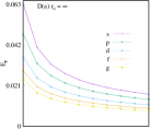
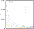
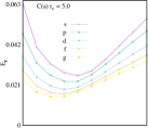
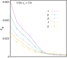
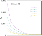
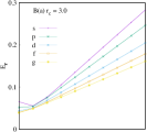
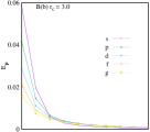
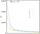
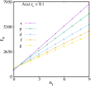
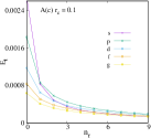
Figure 17.: Plot of $E_{\mathrm{\mathbf{r}}}$ (a), $E_{\mathrm{\mathbf{p}}}$ (b) and $E_{t}$ (c) versus $n_{r}$ (at $\omega=1$) for $s,p,d,f,g$ states at four particular $r_{c}$’s of 3DCHO, namely, $0.1,3,5,\infty$ in panels (A)-(D) [181]. For more details, consult text.

4.4. A Virial-like theorem

Recently a Virial-like equation has been derived by the authors for confined quantum systems [183]. It has the form,

$$\langle\hat{T}^{2}\rangle_{n}-\langle\hat{T}\rangle^{2}_{n} =\langle\hat{V}^{2}\rangle_{n}-\langle\hat{V}\rangle^{2}_{n}$$ (95)

$$(\Delta\hat{T}_{n})^{2} =\langle\hat{V}\rangle_{n}\langle\hat{T}\rangle_{n}-\langle\hat{T}\hat{V}\rangle_{n}=(\Delta\hat{V}_{n})^{2}=\langle\hat{T}\rangle_{n}\langle\hat{V}\rangle_{n}-\langle\hat{V}\hat{T}\rangle_{n}.$$

This relation interprets that, the magnitude of error incurred in $\langle\hat{T}\rangle_{n}$ and $\langle\hat{V}\rangle_{n}$ are identical. Now, one can easily conclude that, $\mathcal{E}_{n}$ is a sum of two average quantities but still provides exact result. It is due to the cancellation of errors between $\langle\hat{T}\rangle_{n}$ and $\langle\hat{V}\rangle_{n}$. In a confinement condition, validity of Eq. (95) can be verified by deriving the expressions of $\langle\hat{T}\hat{V}\rangle_{n,\ell}$, $\langle\hat{V}\hat{T}\rangle_{n,\ell}$, $\langle\hat{V}^{2}\rangle_{n,\ell}$ and $\langle\hat{V}\rangle_{n,\ell}$ (other integrals remain unchanged).

Table 14.: $\mathcal{E}_{n},\left(\Delta V_{n}\right)^{2},\left(\Delta T_{n}\right)^{2},\langle T\rangle_{n}\langle V\rangle_{n}$ $-$ $\langle TV\rangle_{n},\langle T\rangle_{n}\langle V\rangle_{n}$ $-$ $\langle VT\rangle_{n}$ values for $n=0,1$ states in 1DCHO at four ($0.1,0.5,1,\infty$) values of $x_{c}$. See text for detail.

$n$	Property	$x_{c}=0.1$	$x_{c}=0.5$	$x_{c}=1$	$x_{c}=\infty$
	$\mathcal{E}_{0}^{\dagger}$	123.3707084678	4.9511293232	1.2984598320	0.4999999999
	$\left(\Delta V_{0}\right)^{2}$	0.000000600468	0.0003747558	0.0058688193	0.1299999999
0	$\left(\Delta T_{0}\right)^{2}$	0.000000600466	0.0003747558	0.0058688193	0.1299999999
	$\langle T\rangle_{0}\langle V\rangle_{0}-\langle TV\rangle_{0}$	0.000000600466	0.0003747558	0.0058688193	0.1299999999
	$\langle T\rangle_{0}\langle V\rangle_{0}-\langle VT\rangle_{0}$	0.000000600466	0.0003747558	0.0058688193	0.1299999999
	$\mathcal{E}_{1}^{{\ddagger}}$	493.481633417	19.7745341792	5.0755820152	1.499999999
	$\left(\Delta V_{1}\right)^{2}$	0.00000085445	0.00053374630	0.0084865378	0.374999999
1	$\left(\Delta T_{1}\right)^{2}$	0.00000085434	0.00053374630	0.0084865378	0.374999999
	$\langle T\rangle_{1}\langle V\rangle_{1}-\langle TV\rangle_{1}$	0.00000085434	0.00053374630	0.0084865378	0.374999999
	$\langle T\rangle_{1}\langle V\rangle_{1}-\langle VT\rangle_{1}$	0.00000085434	0.00053374630	0.0084865378	0.374999999

${}^{\dagger}$Literature results [34] of $\mathcal{E}_{0}$ for $x_{c}=0.1,0.5,1,\infty$ are: 123.37070846785,

4.9511293232541, 1.2984598320321, 0.5 respectively.

${}^{{\ddagger}}$Literature results [34] of $\mathcal{E}_{1}$ for $x_{c}=0.1,0.5,1,\infty$ are: 493.48163341761,

19.774534179208, 5.0755820152268, 1.5 respectively.

4.4.1. Symmetrically confined harmonic oscillator (SCHO)

In a 1DCHO case, the desired expectation values will take following form:

$$\langle\hat{T}\hat{V}\rangle_{n}=\langle\hat{T}v(x)\rangle_{n}+\langle\hat{T}v_{c}\rangle_{n}=\langle\hat{T}v(x)\rangle_{n}.$$ (96)

One can utilize the property of Reimann integral to simplify,

$$\langle\hat{T}v_{c}\rangle_{n} =\int_{-\infty}^{-x_{c}}\psi^{*}_{n}(x)\hat{T}v_{c}\psi_{n}(x)\mathrm{d}x+$$ (97)

$$\int_{-x_{c}}^{x_{c}}\psi^{*}_{n}(x)\hat{T}v_{c}\psi_{n}(x)\mathrm{d}x+\int_{x_{c}}^{\infty}\psi^{*}_{n}(x)\hat{T}v_{c}\psi_{n}(x)\mathrm{d}x=0$$

The first and third integrals reduce to zero because $\psi_{n}(x)=0$ when $x\geq|x_{c}|$, whereas the second integral leads to zero as, $v_{c}=0$ inside the box. Similarly,

$$\langle\hat{V}\hat{T}\rangle_{n}=\langle v(x)\hat{T}\rangle_{n}+\langle v_{c}\hat{T}\rangle_{n}=\langle v(x)\hat{T}\rangle_{n}$$ (98)

$$\langle\hat{V}^{2}\rangle_{n}=\langle(v(x)^{2}\rangle_{n}+\langle v(x)v_{c}\rangle_{n}+\langle v_{c}v(x)\rangle_{n}+\langle v_{c}^{2}\rangle_{n}=\langle(v(x))^{2}\rangle_{n}$$ (99)

$$\langle\hat{V}\rangle_{n}=\langle v(x)\rangle_{n}+\langle v_{c}\rangle_{n}=\langle v(x)\rangle_{n}.$$ (100)

Thus, for a 1DCHO, with the help of above equations, Eq. (95) may be recast as,

$$\left(\Delta\hat{T}_{n}\right)^{2}=\left(\Delta\hat{V}_{n}\right)^{2}=\langle\hat{T}\rangle_{n}\langle v(x)\rangle_{n}-\langle v(x)\hat{T}\rangle_{n}=\langle\hat{T}\rangle_{n}\langle v(x)\rangle_{n}-\langle\hat{T}v(x)\rangle_{n}.$$ (101)

Thus it is clear from Eq. (101) that, $v_{c}$ does not contribute to the desired expectation values. Hence the only difference between free and enclosed system is that, in latter case, the boundary has been reduced to a finite region from infinity. Representative numerical values of $\mathcal{E}_{n}$, $(\Delta\hat{T}_{n})^{2}$, $(\Delta\hat{V}_{n})^{2}$, $\langle T\rangle_{n}\langle V\rangle_{n}-\langle TV\rangle_{n}$ and $\langle T\rangle_{n}\langle V\rangle_{n}-\langle VT\rangle_{n}$ are produced in Table 14 for $n=0,~{}1$ states of 1DCHO at four selected $x_{c}$ values, namely $0.1,~{}0.5,~{}1,~{}\infty$. In all these four $x_{c}$, $\mathcal{E}_{0}$ and $\mathcal{E}_{1}$ remain in excellent agreement with available literature results as compared in [34], and hence not repeated here. However, no direct reference could be found for expectation values to compare. It is easily noticed that, in both confined and free (last column) scenario, Eq. (95) is obeyed, as all expectation values offer equal values, which affirms the applicability of our newly designed theorem in case of 1DCHO. Additionally, with increase in $x_{c}$, both $\big{(}\Delta\hat{T}\big{)}^{2},\big{(}\Delta\hat{V}\big{)}^{2}$ increase, which presumably occurs as the wave function delocalizes with $x_{c}$. Consequently, the difference between mean square and average values of $\hat{T},~{}\hat{V}$ tends to rise. For more details, please consult [183].

Table 15.: $\mathcal{E}_{n_{r},\ell}$ ,$(\Delta V_{n_{r},\ell})^{2}$ ,$(\Delta T_{n_{r},\ell})^{2}$ ,$\langle T\rangle_{n_{r},\ell}\langle V\rangle_{n_{r},\ell}-\langle TV\rangle_{n_{r},\ell}$ ,$\langle T\rangle_{n_{r},\ell}\langle V\rangle_{n_{r},\ell}-\langle VT\rangle_{n_{r},\ell}$ for $1s,~{}1p,~{}2s$ states in 3DCHO at four specific $r_{c}$’s, such as $0.1,0.5,1,\infty$.

State	Property	$r_{c}=0.1$	$r_{c}=0.5$	$r_{c}=1$	$r_{c}=\infty$
	$\mathcal{E}_{1,0}^{\P}$	493.481633459	19.774534179	5.0755820153	1.4999999
	$\left(\Delta V_{1,0}\right)^{2}$	0.00000085434	0.0005337463	0.0084865378	0.3749999
$1s$	$\left(\Delta T_{1,0}\right)^{2}$	0.00000085434	0.0005337463	0.0084865378	0.3749999
	$\langle T\rangle_{1,0}\langle V\rangle_{1,0}$ $-$ $\langle TV\rangle_{1,0}$	0.00000085434	0.0005337463	0.0084865378	0.3749999
	$\langle T\rangle_{1,0}\langle V\rangle_{1,0}$ $-$ $\langle VT\rangle_{1,0}$	0.00000085434	0.0005337463	0.0084865378	0.3749999
	$\mathcal{E}_{1,1}^{\S}$	1009.53830080	40.428276496	10.282256939	2.4999999
	$\left(\Delta V_{1,1}\right)^{2}$	0.0000008424	0.0005264224	0.0084064867	0.6249999
$1p$	$\left(\Delta T_{1,1}\right)^{2}$	0.00000084238	0.0005264224	0.0084064867	0.6249999
	$\langle T\rangle_{1,1}\langle V\rangle_{1,1}-\langle TV\rangle_{1,1}$	0.00000084238	0.0005264224	0.0084064867	0.6249999
	$\langle T\rangle_{1,1}\langle V\rangle_{1,1}-\langle VT\rangle_{1,1}$	0.00000084238	0.0005264224	0.0084064867	0.6249999
	$\mathcal{E}_{2,0}^{{\ddagger}}$	1973.92248339	78.9969211469	19.899696502	3.4999999
	$\left(\Delta V_{2,0}\right)^{2}$	0.00000182	0.00113739969	0.0181584455	1.6249999
$2s$	$\left(\Delta T_{2,0}\right)^{2}$	0.00000182	0.00113739969	0.0181584455	1.6249999
	$\langle T\rangle_{2,0}\langle V\rangle_{2,0}-\langle TV\rangle_{2,0}$	0.00000182	0.00113739969	0.0181584455	1.6249999
	$\langle T\rangle_{2,0}\langle V\rangle_{2,0}-\langle VT\rangle_{2,0}$	0.00000182	0.00113739969	0.0181584455	1.6249999

${}^{\P}$Literature results [184] of $\mathcal{E}_{1,0}$ for $r_{c}=0.1,0.5,1,\infty$ are: 493.48163346,

19.774534180, 5.0755820154, 1.5 respectively.

${}^{\S}$Literature results [184] of $\mathcal{E}_{1,1}$ for $r_{c}=0.1,0.5,1,\infty$ are: 1009.5383008,

40.428276496, 10.282256939, 2.5 respectively.

${}^{{\ddagger}}$ Literature results [184] of $\mathcal{E}_{2,0}$ for $r_{c}=0.1,0.5,1,\infty$ are: 1973.922483399,

78.996921147, 19.899696502, 3.5 respectively.

4.4.2. 3D Confined harmonic oscillator (3DCHO)

The relevant expectation values for 3DCHO will now take following forms,

$$\langle\hat{T}\hat{V}\rangle_{n_{r},\ell}=\langle\hat{T}v(r)\rangle_{n_{r},\ell}+\langle\hat{T}v_{c}(r)\rangle_{n_{r},\ell}=\langle\hat{T}v(r)\rangle_{n_{r},\ell}.$$ (102)

This happens because $\langle\hat{T}v_{c}(r)\rangle_{n_{r},\ell}=0$, which, in turn occurs, since wave function disappears for $r\geq r_{c}$. A similar argument ($\langle v_{c}(r)\hat{T}\rangle_{n_{r},\ell}=0$) leads to the following relation,

$$\langle\hat{V}\hat{T}\rangle_{n_{r},\ell} = \langle v(r)\hat{T}\rangle_{n_{r},\ell}+\langle v_{c}(r)\hat{T}\rangle_{n_{r},\ell}=\langle v(r)\hat{T}\rangle_{n_{r},\ell}$$ (103)

Then since $\langle v(r)v_{c}(r)\rangle_{n_{r},\ell}=\langle v_{c}(r)v(r)\rangle_{n_{r},\ell}=\langle v_{c}(r)^{2}\rangle_{n_{r},\ell}=0$, we can write,

$$\langle\hat{V}^{2}\rangle_{n_{r},\ell} =\langle v(r)^{2}\rangle_{n_{r},\ell}+\langle v(r)v_{c}(r)\rangle_{n_{r},\ell}+\langle v_{c}(r)v(r)\rangle_{n_{r},\ell}+\langle v_{c}(r)^{2}\rangle_{n_{r},\ell}$$ (104)

$$=\langle v(r)^{2}\rangle_{n_{r},\ell}.$$

And finally, one can derive (since $\langle v_{c}(r)\rangle_{n_{r},\ell}=0$),

$$\langle\hat{V}\rangle_{n_{r},\ell}=\langle v(r)\rangle_{n_{r},\ell}+\langle v_{c}(r)\rangle_{n_{r},\ell}=\langle v(r)\rangle_{n_{r},\ell}.$$ (105)

Thus, for a 3DCHO, Eq. (95) can be recast in to,

$$\langle\hat{T}^{2}\rangle_{n_{r},\ell}-\langle\hat{T}\rangle^{2}_{n_{r},\ell}=\langle\hat{V}^{2}\rangle_{n_{r},\ell}-\langle\hat{V}\rangle^{2}_{n_{r},\ell}$$

$$(\Delta\hat{T}_{n_{r},\ell})^{2}=(\Delta\hat{V}_{n_{r},\ell})^{2}= \langle\hat{T}\rangle_{n_{r},\ell}\langle v(r)\rangle_{n_{r},\ell}-\langle v(r)\hat{T}\rangle_{n_{r},\ell}$$

$$= \langle\hat{T}\rangle_{n_{r},\ell}\langle v(r)\rangle_{n_{r},\ell}-\langle\hat{T}v(r)\rangle_{n_{r},\ell}.$$

This suggests that, similar to 1DCHO, here also the confining potential has no contribution on desired expectation values; only the boundary in confined system gets shifted to $r_{c}$, from $\infty$ of corresponding free counterpart. It clearly supports the validity of Eq. (95) in a 3DCHO. As an illustration, Table 15 imprints numerically calculated expectation values, for three low-lying ($1s,1p,2s$) states at four chosen values of confinement radius, i.e., $0.1,~{}0.5,~{}1,~{}\infty$. This again establishes the efficiency of Eq. (95) for such potential in both confined and free system, as evident from identical values of these quantities at all $r_{c}$’s–last column signifying the corresponding unconstrained system. Accurate energies are quoted from GPS results [184]. No literature is available for average values considered here. Like the 1D case, here also $(\Delta\hat{T}_{n_{r},\ell})^{2},~{}(\Delta\hat{V}_{n_{r},\ell})^{2}$ increase with $r_{c}$. A more detailed discussion may be found in [183].

5. Conclusion

Information-based uncertainty measures like $I,S,R,E$ and several complexities in composite $r,p$ spaces have been employed to understand the effect of confinement in 3DCHO. Before that, we have also discussed $I,S,E$ and various complexities for SCHO and ACHO systems. Apart from that, relative Fisher information for 1DQHO and 3DQHO are reported here. A detailed study reveals that, an SCHO can be considered as an interim model between PIB and 1DQHO. Similarly, a 3DCHO may be treated as a two-mode system; at $r_{c}\rightarrow 0$ it behaves as PISB and at $r_{c}\rightarrow\infty$ it reduces to a 3DQHO.

It is imperative to mention that at $d_{m}=0$, an ACHO reduces to an SCHO. An increase in $d_{m}$ leads to localization of the system in real space. $S_{x},S_{p}$ can completely interpret the competing nature of ACHO potential. In contrast, $I_{x},I_{p}$ prove inefficient for such analysis. Further, $E_{x},E_{p}$ provide important knowledge which guides the reader to a better understanding of such systems.

In 3DCHO, at very low $r_{c}$, $R_{\mathrm{\mathbf{r}}}^{\alpha}$, $S_{\mathrm{\mathbf{r}}}$ reduce and $E_{\mathrm{\mathbf{r}}}$ grows up as $n_{r}$ progresses. This behavior clearly suggests that the effect of confinement accelerates with increase of number of nodes in the system. In future, it will be interesting to study the effect of penetrable boundary on such systems. Further, study of relative information for SCHO, ACHO and 3DCHO systems would be highly desirable.

6. Acknowledgement

The authors express their sincere gratitude to Prof. Nadya S. Columbus, President, NOVA Science Publishers, NY, USA, for the kind invitation to present our work in this exciting area. We are extremely thankful to the Editor, Prof. Yilun Shang for giving us the opportunity to contribute and also extending the submission deadline generously. AKR gratefully acknowledges financial support from SERB, Department of Science and Technology (DST), New Delhi (sanction no. EMR/2014/000838). NM thanks DST for financial support through NPDF grant (PDF/2016/000014CS). It is a pleasure to thank Ms. Sangita Majumdar for giving a careful reading of the manuscript.

References

- Michels, A.; De Boer, J.; Bijl, A. [1937] Michels, A.; De Boer, J.; Bijl, A. (1937). Remarks concerning molecular interaction and their influence on the polarizability. Physica 4, 981.
- Jaskólski, W. [1996] Jaskólski, W. (1996). Confined many-electron systems. Phys. Rep. 271, 1.
- Dolmatov, V. K.; Baltenkov, A. S.; Connerade, J.-P; Mason, S. T. [2004] Dolmatov, V. K.; Baltenkov, A. S.; Connerade, J.-P; Mason, S. T. (2004). Structure and photoionization of confined atoms. Radiat. Phys. Chem. 70, 417.
- Sabin, J., Brändas, E.; and Cruz, S. [2009] Sabin, J., Brändas, E.; and Cruz, S. (Ed.) (2009). Adv. Quant. Chem., Volume 57 & 58. New York: Academic Press.
- Sen, K. D. [2014] Sen, K. D. (Ed.) (2014). Electronic Structure of Quantum Confined Atoms and Molecules. Switzerland: Springer International Publishing.
- Ley-Koo, E. [2018] Ley-Koo, E. (2018). Recent progress in confined atoms and molecules: superintegrability and symmetry breakings. Revista Mexicana de Física 64, 326.
- Dolmatov, V. K. [2009] Dolmatov, V. K. (2009). Photoionization of atoms encaged in spherical fullerenes. Adv. Quant. Chem. 58, 13.
- Charkin, O. P.; Klimenko, N. M.; Charkin, D. O. [2009] Charkin, O. P.; Klimenko, N. M.; Charkin, D. O. (2009). DFT study of molecules confined inside fullerene and fullerene-like cages. Adv. Quant. Chem. 58, 69.
- Etindele, A. J.; Maezono, R.; Melingui-Melono, R. L.; Motapon, O. [2017] Etindele, A. J.; Maezono, R.; Melingui-Melono, R. L.; Motapon, O. (2017). Influence of endohedral confinement of atoms on structural and dynamical properties of the fullerene. Chem. Phys. Lett. 685, 395.
- Auluck, F. C. [1941a] Auluck, F. C. (1941a). Energy levels of an artificially bounded linear oscillator. Proc. Nat. Inst. Sci. India 7, 133.
- Auluck, F. C. [1941b] Auluck, F. C. (1941b). The Artificially Bounded Relativistic Linear Oscillator. Proc. Nat. Inst. Sci. India 7, 383.
- Chandrasekhar, S. [1943] Chandrasekhar, S. (1943). Dynamical friction. II. the rate of escape of stars from clusters and the evidence for the operation of dynamical friction. Astrophys. J. 97, 263.
- Dingle, R. B. [1952a] Dingle, R. B. (1952a). Some magnetic properties of metals III. Diamagnetic resonance. Proc. Royal Soc. London A 212, 38.
- Dingle, R. B. [1952b] Dingle, R. B. (1952b). Some magnetic properties of metals IV. Properties of small systems of electrons. Proc. Royal Soc. London A 212, 47.
- Grinberg, M.; Jaskólski, W.; Koepke, Cz.; Planelles, J.; Janowicz, M. [1994] Grinberg, M.; Jaskólski, W.; Koepke, Cz.; Planelles, J.; Janowicz, M. (1994). Spectroscopic manifestation of a confinement-type lattice anharmonicity. Phys. Rev. B 50, 6504(R).
- Auluck, F. C.; Kothari, D. S. [1945] Auluck, F. C.; Kothari, D. S. (1945). The quantum mechanics of a bounded linear harmonic oscillator. Proc. Cambridge Phil. Soc. 41, 175.
- Baijal, J. S.; Singh, K. K. [1955] Baijal, J. S.; Singh, K. K. (1955). The energy levels and transition probabilities for a bounded linear harmonic oscillator. Prog. Theor. Phys. (Kyoto) 14, 214.
- Hull, T. E.; Julius, R. S. [1956] Hull, T. E.; Julius, R. S. (1956). Enclosed quantum mechanical systems. Can. J. Phys. 34, 914.
- Dean, P. [1966] Dean, P. (1966). The constrained quantum mechanical harmonic oscillator. Proc. Cambridge Phil. Soc. 62, 277.
- Vawter, R. [1968] Vawter, R. (1968). Effects of finite boundaries in a one-dimensional harmonic oscillator. Phys. Rev. 174, 749.
- Vawter, R. [1973] Vawter, R. (1973). Energy eigenvalues of a bounded centrally located harmonic oscillator. J. Math. Phys. 14, 1864.
- Consortini, A.; Frieden, B. R. [1976] Consortini, A.; Frieden, B. R. (1976). Quantum-mechanical solution for the simple harmonic oscillator in a box. Nuovo Cimento B 35, 153.
- Aguilera-Navarro, V.C.; Ley-Koo, E.; Zimerman, A. H. [1980] Aguilera-Navarro, V.C.; Ley-Koo, E.; Zimerman, A. H. (1980). Perturbative, asymptotic and Padé-approximant solutions for harmonic and inverted oscillators in a box. J. Phys. A 13, 3585.
- Fernández, F. M.; Castro, E. A. [1981a] Fernández, F. M.; Castro, E. A. (1981a). Hyper-virial analysis of enclosed quantum mechanical systems. I. Dirichlet boundary conditions. Int. J. Quant. Chem. 19, 521.
- Fernández, F. M.; Castro, E. A. [1981b] Fernández, F. M.; Castro, E. A. (1981b). Hyper-virial analysis of enclosed quantum mechanical systems. III. Unsymmetrical boundary conditions. Int. J. Quant. Chem. 20, 623.
- Arteca, G. A.; Maluendes, S. A.; Fernández, F. M.; Castro, E. A. [1983] Arteca, G. A.; Maluendes, S. A.; Fernández, F. M.; Castro, E. A. (1983). Discussion of several analytical expressions for the eigenvalues of the bounded harmonic oscillator and hydrogen atom. Int. J. Quant. Chem. 24, 169.
- Taşeli, H. [1993] Taşeli, H. (1993). Accurate computation of the energy spectrum for potentials with multiminima. Int. J. Quant. Chem. 46, 319.
- Vargas, R.; Garza, J.; Vela, A.; [1996] Vargas, R.; Garza, J.; Vela, A.; (1996). Strongly convergent method to solve one-dimensional quantum problems. Phys. Rev. E 53, 1954.
- Sinha, A.; Roychoudhury, R. [1999] Sinha, A.; Roychoudhury, R. (1999). WKB and MAF quantization rules for spatially confined quantum mechanical systems. J. Math. Chem. 73, 497.
- Sinha, A. [2000] Sinha, A. (2000). SWKB formalism for confined quantum systems. Int. J. Quant. Chem. 79, 267.
- Montgomery Jr., H. E.; Campoy, G.; Aquino, N. [2010] Montgomery Jr., H. E.; Campoy, G.; Aquino, N. (2010). The confined N-dimensional harmonic oscillator revisited. Phys. Scr. 81, 045010.
- Campoy, G.; Aquino, N.; Granados, V. N. [2002] Campoy, G.; Aquino, N.; Granados, V. N. (2002). Energy eigenvalues and Einstein coefficients for the one-dimensional confined harmonic oscillators. J. Phys. A 35, 4903.
- Amore, P.; Fernández, F. M. [2010] Amore, P.; Fernández, F. M. (2010). One-dimensional oscillator in a box. Eur. J. Phys. 31, 69.
- Roy, A. K. [2015] Roy, A. K. (2015). Quantum confinement in 1D systems through an imaginary-time evolution method. Mod. Phys. Lett. A 37, 1550176.
- Aquino, N.; Cruz, E. [2017] Aquino, N.; Cruz, E. (2017). The 1-dimensional confined harmonic oscillator revisited. Revista Mexicana de Física 63, 580.
- Aquino, N.; Castaño, E.; Campoy, G.; Granados, V. [2001] Aquino, N.; Castaño, E.; Campoy, G.; Granados, V. (2001). Einstein coefficients and dipole moment for the asymmetrically confined harmonic oscillator. Eur. J. Phys. 22, 645.
- Fernández, F. M.; Castro, E. A. [1981] Fernández, F. M.; Castro, E. A. (1981). Hyper-virial treatment of multidimensional isotropic bounded oscillators. Phys. Rev. A 24, 2883.
- Aguilera-Navarro, V. C.; Gomes, J. F.; Zimerman, A. H.; Ley-Koo, E. [1983] Aguilera-Navarro, V. C.; Gomes, J. F.; Zimerman, A. H.; Ley-Koo, E. (1983). On the radius of convergence of Rayleigh-Schrödinger perturbative solutions for quantum oscillators in circular and spherical boxes. J. Phys. A 16, 2943.
- Marin, J. L.; Cruz, S. A. [1991] Marin, J. L.; Cruz, S. A. (1991). On the use of direct variational methods to study confined quantum systems. Am. J. Phys. 59, 931.
- Dutt, R.; Mukherjee, A.; Varshni, Y. P. [1995] Dutt, R.; Mukherjee, A.; Varshni, Y. P. (1995). Supersymmetric semiclassical approach to confined quantum problems. Phys. Rev. A 52, 1750.
- Taşeli, H.; Zafer, A. [1997a] Taşeli, H.; Zafer, A. (1997a). A Fourier-Bessel expansion for solving radial Schrödinger equation in two dimensions. Int. J. Quant. Chem. 61, 759.
- Taşeli, H.; Zafer, A. [1997b] Taşeli, H.; Zafer, A. (1997b). Bessel basis with applications: N-dimensional isotropic polynomial oscillators. Int. J. Quant. Chem. 63, 936.
- Aquino, N. [1997] Aquino, N. (1997). The isotropic bounded oscillators. J. Phys. A 30, 2403.
- Sinha, A. [2003] Sinha, A. (2003). Three-dimensional confinement: WKB revisited. J. Math. Chem. 34, 201.
- Filho, E. D.; Ricotta, R. M. [2003] Filho, E. D.; Ricotta, R. M. (2003). Supersymmetric variational energies of 3D confined potentials. Phys. Lett. A 320, 95.
- Sen, K. D.; Roy, A. K. [2006] Sen, K. D.; Roy, A. K. (2006). Studies on the 3D confined potentials using generalized pseudospectral approach. Phys. Lett. A 357, 112.
- Roy [2014] Roy, A. K. (2014). Confinement in 3D polynomial oscillators through a generalized pseudospectral method. Mod. Phys. Lett. A 29, 1450104.
- Stevanović, Lj.; Sen, K. D. [2008a] Stevanović, Lj.; Sen, K. D. (2008a). A study of the confined 2D isotropic harmonic oscillator in terms of the annihilation and creation operators and the infinitesimal operators of the SU(2) group. J. Phys. A 41, 265203.
- Stevanović, Lj.; Sen, K. D. [2008b] Stevanović, Lj.; Sen, K. D. (2008b). Eigenspectrum properties of the confined 3D harmonic oscillator. J. Phys. A 41, 225002.
- Serrano, F. A.; Dong, S.-H. [2013] Serrano, F. A.; Dong, S.-H. (2013). Proper quantization rule approach to three-dimensional quantum dots. Int. J. Quant. Chem. 113, 2282.
- Al-Jaber, S. M. [2008] Al-Jaber, S. M. (2008). A confined N-dimensional harmonic oscillator. Int. J. Theor. Phys. 47, 1853.
- Montgomery, Jr., H. E.; Aquino, N. A.; Sen, K. D. [2007] Montgomery, Jr., H. E.; Aquino, N. A.; Sen, K. D. (2007). Degeneracy of confined D-dimensional harmonic oscillator. Int. J. Quant. Chem. 107, 798.
- Poland, D. [2000] Poland, D. (2000). Maximum-entropy calculation of energy distributions. J. Chem. Phys. 112, 6554.
- Singer, A. [2004] Singer, A. (2004). Maximum entropy formulation of the Kirkwood superposition approximation. J. Chem. Phys. 121, 3657.
- Antoniazzi, A.; Fanelli, D.; Barré, J.; Chavanis, P.-H.; Dauxois, T.; Ruffo, S. [2007] Antoniazzi, A.; Fanelli, D.; Barré, J.; Chavanis, P.-H.; Dauxois, T.; Ruffo, S. (2007). Maximum entropy principle explains quasistationary states in systems with long-range interactions: The example of the Hamiltonian mean-field model. Phys. Rev. E 75, 011112.
- Bialyniki-Birula, I.; Mycielski, J. [1975] Bialyniki-Birula, I.; Mycielski, J. (1975). Uncertainty relation for information entropy in wave mechanics. Commun. Math. Phys. 44, 129.
- Shannon [1951] Shannon, C. E. (1951). Prediction and entropy of printed english. Bell System Technical J. 30, 50.
- Bialyniki-Birula, I. [2006] Bialyniki-Birula, I. (2006). Formulation of uncertainty relations in terms of the Rényi entropies. Phys. Rev. A 74, 052101.
- Duan, L.-M.; Giedke. G.; Cirac, J. I.; Zoller, P. [2000] Duan, L.-M.; Giedke. G.; Cirac, J. I.; Zoller, P. (2000). Inseparability criterion for continuous variable systems. Phys. Rev. Lett. 84, 2722.
- Simon [2000] Simon, R. (2000). Peres-Horodecki separability criterion for continuous variable systems. Phys. Rev. Lett. 84, 2726.
- Roy [2004a] Roy, A. K. (2004a). Calculation of the spiked harmonic oscillators through a generalized pseudospectral method. Phys. Lett. A 321, 231.
- Roy [2004b] Roy, A. K. (2004b). Calculation of the bound states of power-law and logarithmic potentials through a generalized pseudospectral method. J. Phys. G 30, 269.
- Roy [2004c] Roy, A. K. (2004c). Studies on the hollow states of atomic lithium using a density functional approach. J. Phys. B 37, 4569.
- Roy [2005a] Roy, A. K. (2005a). The generalized pseudospectral approach to the bound states of Húlthen and Yukawa potential. Pramana-J. Phys. 65, 1.
- Roy [2005b] Roy, A. K. (2005b). Studies on some singular potentials in quantum mechanics. Int. J. Quant. Chem. 104, 861.
- Roy [2005c] Roy, A. K. (2005c). Density functional studies on the hollow resonances in Li-isoelectronic sequence (Z=4-10). J. Phys. B 38, 1591.
- Roy, A. K.; Jalbout, A. F. [2007] Roy, A. K.; Jalbout, A. F. (2007). Ground and excited states of Li, Be through a density-based approach. Chem. Phys. Lett. 445, 355.
- Roy, A. K.; Jalbout, A. F.; Proynov, E. I. [2008a] Roy, A. K.; Jalbout, A. F.; Proynov, E. I. (2008a). Accurate calculation of the bound states of hellmann potential. J. Math. Chem. 44, 260.
- Roy, A. K.; Jalbout, A. F.; Proynov, E. I. [2008b] Roy, A. K.; Jalbout, A. F.; Proynov, E. I. (2008b). Bound state spectra of the 3D rational potential. Int. J. Quant. Chem. 108, 827.
- Roy, A. K.; Jalbout, A. F. [2008] Roy, A. K.; Jalbout, A. F. (2008). Bound states of the generalized spiked harmonic oscillator. J. Mol. Struct. (Theochem) 853, 27.
- Roy [2013a] Roy, A. K. (2013a). Studies on some exponential-screened Coulomb potentials. Int. J. Quant. Chem. 113, 1503.
- Roy [2013b] Roy, A. K. (2013b). Accurate ro-vibrational spectroscopy of diatomic molecules in a Morse oscillator potential. Results in Physics 3, 103.
- Roy [2014a] Roy, A. K. (2014a). Studies on the bound-state spectrum of Hyperbolic potential. Few-Body Systems 55, 143.
- Roy [2014b] Roy, A. K. (2014b). Ro-vibrational studies of diatomic molecules in a shifted Deng-Fan oscillator potential. Int. J. Quant. Chem. 114, 383.
- Roy [2014c] Roy, A. K. (2014c). Studies on bound-state spectra of Manning-Rosen potential. Mod. Phys. Lett. A 29, 1450042.
- Roy [2014d] Roy, A. K. (2014d). Ro-vibrational spectroscopy of molecules represented by Tietz-Hua oscillator potential. J. Math. Chem 52, 1405.
- Roy [2015] Roy, A. K. (2015). Spherical confinement of Coulombic systems inside an impenetrable box: H atom and the Húlthen potential. Int. J. Quant. Chem. 115, 937.
- Roy [2016] Roy, A. K. (2016). Critical parameters and spherical confinement of H atoms in screened Coulomb potential. Int. J. Quant. Chem. 116, 953.
- Abramowitz, M.; Stegun, I. [1964] Abramowitz, M.; Stegun, I. (1964). Handbook of Mathematical Functions. New York: Dover.
- Anderson; J. B. [1975] Anderson; J. B. (1975). A randon-walk simulation of the Schrödinger equation: H. J. Chem. Phys. 63, 1499.
- Kosloff, R.; Tal-Ezer, H. [1986] Kosloff, R.; Tal-Ezer, H. (1986). A direct relaxation method for calculating eigenfunctions and eigenvalues of the Schrödinger equation on a grid. Chem. Phys. Lett. 127, 223.
- Lehtovaara, L.; Toivanen, J.; Eloranta, J. [2007] Lehtovaara, L.; Toivanen, J.; Eloranta, J. (2007). Solution of time-dependent Schrödinger equation by the imaginary-time propagation method. J. Comput. Phys. 221, 148.
- Chin, S. A.; Janecek, S.; Krotscheck, S. [2009] Chin, S. A.; Janecek, S.; Krotscheck, S. (2009). Any order imaginary time propagation method for solving the Schrödinger equation. Chem. Phys. Lett. 470, 342.
- Sudiarta, I. W.; Wallace Geldart, D. J. [2009] Sudiarta, I. W.; Wallace Geldart, D. J. (2009). The finite difference time domain method for computing the single-particle density matrix. J. Phys. A 42, 285002.
- Strickland, M.; Yager-Elorriaga, D. [2010] Strickland, M.; Yager-Elorriaga, D. (2010). A parallel algorithm for solving the 3d Schrödinger equation. J. Comput. Phys. 229, 6015.
- Luukko, P. J. J.; Räsänen, E. [2013] Luukko, P. J. J.; Räsänen, E. (2013). Imaginary time propagation code for large-scale two-dimensional eigenvalue problems in magnetic fields. Comput. Phys. Commun. 184, 769.
- Roy, A. K.; Dey, B. K.; Deb, B. M. [1999] Roy, A. K.; Dey, B. K.; Deb, B. M. (1999). Direct calculation of ground-state electronic densities and properties of noble gas atoms through a single time-dependent hydrodynamical equation. Chem. Phys. Lett. 308, 523.
- Roy, A. K.; Chu, S. I. [2002] Roy, A. K.; Chu, S. I. (2002). Quantum fluid dynamics approach for electronic structure calculation: Application to the study of ground-state properties of rare gas atoms. J. Phys. B 35, 2075.
- Roy A. K.; Gupta N.; Deb B. M. [2002] Roy A. K.; Gupta N.; Deb B. M. (2002). Time-dependent quantum-mechanical calculation of ground and excited states of anharmonic and double-well oscillators. Phys. Rev. A 65, 012109.
- Gupta N.; Roy A. K.; Deb, B. M. [2002] Gupta N.; Roy A. K.; Deb, B. M. (2002). One-dimensional multiple-well oscillators: A time-dependent quantum mechanical approach. Pramana J. Phys. 59, 575.
- Wadehra, A.; Roy, A. K.; Deb, B. M. [2003] Wadehra, A.; Roy, A. K.; Deb, B. M. (2003). Ground and excited states of one-dimensional self-interacting nonlinear oscillators through time-dependent quantum mechanics. Int. J. Quant. Chem. 91, 597.
- Roy, A. K.; Thakkar, A. J.; Deb, B. M. [2005] Roy, A. K.; Thakkar, A. J.; Deb, B. M. (2005). Low-lying states of two-dimensional double-well potentials. J. Phys. A 38, 2189.
- Roy [2014] Roy, A. K. (2014). Ground and excited states of spherically symmetric potentials through an imaginary-time evolution method: application to spiked harmonic oscillators. J. Math. Chem 52, 2645.
- Hammond, B. L.; Lester Jr., W. A.; Reynolds, P. J. [1994] Hammond, B. L.; Lester Jr., W. A.; Reynolds, P. J. (1994). Monte Carlo Methods in Ab Initio Quantum Chemistry. Singapore: World Scientific.
- Roy, A. K.; Chu, S. I. [2002a] Roy, A. K.; Chu, S. I. (2002a). Density functional calculations on singly- and doubly-excited rydberg states of many-electron systems. Phys. Rev. A 65, 052508.
- Roy, A. K.; Chu, S. I. [2002b] Roy, A. K.; Chu, S. I. (2002b). Quantum fluid dynamics approach for strong field processes: Aapplication to the study of multiphoton ionization and high-order harmonic generation of He and Ne in intense laser fields. Phys. Rev. A 65, 043402.
- Mukherjee, N; Roy, A. K. [2018] Mukherjee, N; Roy, A. K. (2018). Information-entropic measures in free and confined hydrogen atom. Int. J. Quant. Chem. 118, e25596.
- Cover, T. M.; Thomas, J. A. [2006] Cover, T. M.; Thomas, J. A. (2006). Elements of Information Theory. New York: John Wiley & Sons, Ltd.
- Nielsen, M. A.; Chuang, I. L. [2010] Nielsen, M. A.; Chuang, I. L. (2010). Quantum Computation and Quantum Information. Cambridge: Cambridge University Press.
- Ramírez, J. C.; Soriano, C.; Esquivel, R. O.; Sagar, R. P.; Hô, M.; Smith, V. H. [1997] Ramírez, J. C.; Soriano, C.; Esquivel, R. O.; Sagar, R. P.; Hô, M.; Smith, V. H. (1997). Jaynes information entropy of small molecules: Numerical evidence of the Collins conjecture. Phys. Rev. A 56, 4477.
- Delle, L. S. [2015] Delle, L. S. (2015). Shannon entropy and many-electron correlations: Theoretical concepts, numerical results, and Collins conjecture. Int. J. Quant. Chem. 115, 1396.
- Ghiringhelli, L. M.; Hamilton, I. P.; Delle, L. S [2010] Ghiringhelli, L. M.; Hamilton, I. P.; Delle, L. S (2010). Interacting electrons, spin statistics, and information theory. J. Chem. Phys. 132, 014106.
- Ghiringhelli, L. M.; Delle, L. S.; Mosna, R. A.; Hamilton, I. P. [2010] Ghiringhelli, L. M.; Delle, L. S.; Mosna, R. A.; Hamilton, I. P. (2010). Information-theoretic approach to kinetic-energy functionals: the nearly uniform electron gas. J. Math. Chem. 48, 78.
- Nagy, Á. [2014] Nagy, Á. (2014). Fisher and Shannon information in orbital-free density functional theory. Int. J. Quant. Chem. 115, 1392.
- Alipour, M. [2015] Alipour, M. (2015). Making a happy match between orbital-free density functional theory and information energy density. Chem. Phys. Lett. 635, 210.
- Delle, L. S. [2009a] Delle, L. S. (2009a). On the scaling properties of the correlation term of the electron kinetic functional and its relation to the Shannon measure. Euro Phys. Lett. 86, 40004.
- Delle, L. S. [2009b] Delle, L. S. (2009b). Erratum: On the scaling properties of the correlation term of the electron kinetic functional and its relation to the Shannon measure. Euro Phys. Lett. 88, 19901.
- Mohajeri, A.; Alipour, M. [2009] Mohajeri, A.; Alipour, M. (2009). Information energy as an electron correlation measure in atomic and molecular systems. Int. J. Quantum Inf. 07, 801.
- Grassi, A. [2011] Grassi, A. (2011). A relationship between atomic correlation energy of neutral atoms and generalized entropy. Int. J. Quant. Chem. 111, 2390.
- Flores-Gallegos, N. [2016] Flores-Gallegos, N. (2016). Informational energy as a measure of electron correlation. Chem. Phys. Lett. 666, 62.
- Alipour, M.; Badooei, Z. [2018] Alipour, M.; Badooei, Z. (2018). Toward electron correlation and electronic properties from the perspective of information functional theory. J. Phys. Chem. A 122, 6424.
- Barghathi, H.; Herdman, C.; Maestro, A. D. [2018] Barghathi, H.; Herdman, C.; Maestro, A. D. (2018). Rényi generalization of the accessible entanglement entropy. Phys. Rev. Lett. 121, 150501.
- Noorizadeh, S.; Shakerzadeh, E. [2010] Noorizadeh, S.; Shakerzadeh, E. (2010). Shannon entropy as a new measure of aromaticity, Shannon aromaticity. Phys. Chem. Chem. Phys. 12, 4742.
- Rényi, A. [1961] Rényi, A. (1961). On measures of entropy and information. Proc. Fourth Berkeley Symp. on Math. Statist. and Prob., 547.
- Rényi, A. [1970] Rényi, A. (1970). Probability Theory. Amsterdam: North-Holland Pub. Company.
- Varga, I.; Pipek, J. [2003] Varga, I.; Pipek, J. (2003). Rényi entropies characterizing the shape and the extension of the phase space representation of quantum wave functions in disordered systems. Phys. Rev. E 68, 026202.
- Renner, R.; Gisin, N.; Kraus. B. [2005] Renner, R.; Gisin, N.; Kraus. B. (2005). Information-theoretic security proof for quantum-key-distribution protocols. Phys. Rev. A 72, 012332.
- Lévay, P.; Nagy, S.; Pipek, J. [2005] Lévay, P.; Nagy, S.; Pipek, J. (2005). Elementary formula for entanglement entropies of fermionic systems. Phys. Rev. A 72, 022302.
- Verstraete, F.; Cirac, J. I. [2006] Verstraete, F.; Cirac, J. I. (2006). Matrix product states represent ground states faithfully. Phys. Rev. B 73, 094423.
- Bialas, A.; Czyz, W.; Zalewski, K. [2006] Bialas, A.; Czyz, W.; Zalewski, K. (2006). Moments of the Wigner function and Rényi entropies at freeze-out. Phys. Rev. C 73, 034912.
- Salcedo, L. L. [2009] Salcedo, L. L. (2009). Phase-space localization of antisymmetric functions. J. Math. Phys. 50, 012106.
- Nagy, Á.; Romera. E. [2009] Nagy, Á.; Romera. E. (2009). Maximum Rényi entropy principle and the generalized Thomas-Fermi model. Phys. Lett. A 373, 844.
- McMinis, J.; Tubman, N. M. [2013] McMinis, J.; Tubman, N. M. (2013). Rényi entropy of the interacting fermi liquid. Phys. Rev. B 87, 081108(R).
- Liu, S.-B.; Rong, C.-Y.; Wu, Z.-M.; Lu, T. [2015] Liu, S.-B.; Rong, C.-Y.; Wu, Z.-M.; Lu, T. (2015). Moments of the Wigner function and Rényi entropies at freeze-out. Acta. Phys. Chim. Sin. 31, 2057.
- Kim, I. [2018] Kim, I. (2018). Rényi- entropies of quantum states in closed form: Gaussian states and a class of non-Gaussian states. Phys. Rev. E 97, 062141.
- Frieden [2004] Frieden, B. R. (2004). Science from Fisher Information: A Unification. Cambridge: Cambridge University Press.
- Sen, K. D. [2011] Sen, K. D. (Ed.) (2011). Statistical Complexity: Applications in Electronic Structure. Netherland: Springer International Publishing.
- Romera, E.; Sánchez-Moreno, P.; Dehesa, J. S. [2005] Romera, E.; Sánchez-Moreno, P.; Dehesa, J. S. (2005). The Fisher information of single-particle systems with a central potential. Chem. Phys. Lett. 414, 468.
- Mukherjee, N.; Majumdar, S.; Roy, A. K. [2018] Mukherjee, N.; Majumdar, S.; Roy, A. K. (2018). Fisher information in confined hydrogen-like ions. Chem. Phys. Lett. 691, 449.
- Mukherjee, N.; Roy, A. K. [2018] Mukherjee, N.; Roy, A. K. (2018). Fisher information in confined isotropic harmonic oscillator. Int. J. Quant. Chem. 118, e25727.
- Patil, S. H.; Sen, K. D.; Watson, N. A.; Montgomery Jr., H. E. [2007] Patil, S. H.; Sen, K. D.; Watson, N. A.; Montgomery Jr., H. E. (2007). Characteristic features of net information measures for constrained Coulomb potentials. J. Phys. B 40, 2147.
- Ghosal, A.; Mukherjee, N.; Roy, A. K. [2016] Ghosal, A.; Mukherjee, N.; Roy, A. K. (2016). Information-entropic measures of a quantum harmonic oscillator in symmetric and asymmetric confinement within an impenetrable box. Ann. Phys. (Berlin) 528, 796.
- Onicescu, O. [1966] Onicescu, O. (1966). Energie informationnelle. Comptes Rendus Hebdomadaires des Seances de l’Academie des Sciences Serie A 263, 841.
- Pardo, L. [1986] Pardo, L. (1986). Order- weighted information energy. Info. Sciences 40, 155.
- Bhatia, P. [1997] Bhatia, P. (1997). On measures of information energy. Info. Sciences 97, 233.
- Noughabi, H. A.; Chahkandi, M. [2015] Noughabi, H. A.; Chahkandi, M. (2015). Informational energy and its application in testing normality. Ann. Data Sci. 2, 391.
- Alcoba, D. R.; Torre, A.; Lain, L.; Massaccesi, G. E.; Oña, O. B.; Ayers, P. W.; Van Raemdonck, M.; Bultinck, P.; Van Neck, D. [2016] Alcoba, D. R.; Torre, A.; Lain, L.; Massaccesi, G. E.; Oña, O. B.; Ayers, P. W.; Van Raemdonck, M.; Bultinck, P.; Van Neck, D. (2016). Performance of Shannon-entropy compacted N-electron wave functions for configuration interaction methods. Theor. Chem. Acc. 135, 153.
- Zozor, S.; Portesi, M.; Vignat, C. [2008] Zozor, S.; Portesi, M.; Vignat, C. (2008). Some extensions of the uncertainty principle. Physica A 387, 4800.
- Shiner, J. S.; Landsberg, P. T.; Davison, M. [1999] Shiner, J. S.; Landsberg, P. T.; Davison, M. (1999). Simple measure for complexity. Phys. Rev. E 59, 1459.
- Catalán, R. G.; Garay, J.; López-Ruiz, R. [2002] Catalán, R. G.; Garay, J.; López-Ruiz, R. (2002). Features of the extension of a statistical measure of complexity to continuous systems. Phys. Rev. E 66, 11102.
- Sánchez, J. R.; López-Ruiz, R. [2005] Sánchez, J. R.; López-Ruiz, R. (2005). A method to discern complexity in two-dimensional patterns generated by coupled map lattices. Physica A 355, 633.
- Landsberg, P. T.; Shiner; J. S. [1998] Landsberg, P. T.; Shiner; J. S. (1998). Disorder and complexity in an ideal non-equilibrium fermi gas. Phys. Lett. A 245, 228.
- Romera, E.; Dehesa, J. S. [2004] Romera, E.; Dehesa, J. S. (2004). The Fisher-Shannon information plane, an electron correlation tool. J. Chem. Phys. 120, 8906.
- Sen, K. D.; Antolín, J.; Angulo, J. C. [2007] Sen, K. D.; Antolín, J.; Angulo, J. C. (2007). Fisher-Shannon analysis of ionization processes and isoelectronic series. Phys. Rev. A 76, 032502.
- Sen, K. D.; Antolín, J.; Angulo, J. C. [2008] Sen, K. D.; Antolín, J.; Angulo, J. C. (2008). Fisher-Shannon plane and statistical complexity of atoms. Phys. Rev. A 372, 670.
- Antolín, J.; Angulo, J. C. [2009] Antolín, J.; Angulo, J. C. (2009). Complexity analysis of ionization processes and isoelectronic series. Int. J. Quant. Chem. 109, 586.
- Calbet, X.; López-Ruiz, R. [2001] Calbet, X.; López-Ruiz, R. (2001). Tendency towards maximum complexity in a nonequilibrium isolated system. Phys. Rev. E 63, 066116.
- Martin, M. T.; Plastino, A.; Rosso, A. O. [2006] Martin, M. T.; Plastino, A.; Rosso, A. O. (2006). Generalized statistical complexity measures: Geometrical and analytical properties. Physica A 369, 439.
- Romera E., Nagy, Á. [2008] Romera E., Nagy, Á. (2008). Rényi information of atoms. Phys. Lett. A 372, 4918.
- Angulo, J. C.; Antolín, J. [2008] Angulo, J. C.; Antolín, J. (2008). Atomic complexity measures in position and momentum spaces. J. Chem. Phys. 128, 164109.
- Esquivel, R. O.; Angulo, J. C.; Antolín, J.; Dehesa, J. S.; López-Rosa, S.; Flores-Gallegos, N. [2010] Esquivel, R. O.; Angulo, J. C.; Antolín, J.; Dehesa, J. S.; López-Rosa, S.; Flores-Gallegos, N. (2010). Analysis of complexity measures and information planes of selected molecules in position and momentum spaces. Phys. Chem. Chem. Phys. 12, 7108.
- Welearegay, M. A.; Balawender, R.; Holas A. [2014] Welearegay, M. A.; Balawender, R.; Holas A. (2014). Information and complexity measures in molecular reactivity studies. Phys. Chem. Chem. Phys. 16, 14928.
- Esquivel, R. O.; Molina-Espíritu, M.; Angulo, J. C.; Antolín, J.; Flores-Gallegos, N.; Dehesa, J. S. [2011] Esquivel, R. O.; Molina-Espíritu, M.; Angulo, J. C.; Antolín, J.; Flores-Gallegos, N.; Dehesa, J. S. (2011). Information-theoretical complexity for the hydrogenic abstraction reaction. Mol. Phys. 109, 2353.
- Molina-Espíritu, M.; Esquivel, R. O.; Angulo, J. C.; Antolín, J.; Dehesa, J. S. [2012] Molina-Espíritu, M.; Esquivel, R. O.; Angulo, J. C.; Antolín, J.; Dehesa, J. S. (2012). Information-theoretical complexity for the hydrogenic identity exchange reaction. J. Math. Chem. 50, 1882.
- Esquivel, R. O.; Molina-Espíritu, M.; Dehesa, J. S.; Angulo, J. C.; Antolín, J. [2012] Esquivel, R. O.; Molina-Espíritu, M.; Dehesa, J. S.; Angulo, J. C.; Antolín, J. (2012). Concurrent phenomena at the transition region of selected elementary chemical reactions: An information‐theoretical complexity analysis. Int. J. Quant. Chem. 112, 3578.
- Kullback, S.; Leibler, R. A. [1951] Kullback, S.; Leibler, R. A. (1951). On information and sufficiency. Ann. Math. Stat. 22, 79.
- Kullback, S. [1959] Kullback, S. (1959). Information Theory and Statistics. New York: John Wiley & Sons.
- Sagar, R. P.; Guevara, N. L. [2008] Sagar, R. P.; Guevara, N. L. (2008). Relative entropy and atomic structure. J. Mol. Struct. (Theochem) 857, 72.
- Nagy, Á.; Romera, E. [2009] Nagy, Á.; Romera, E. (2009). Relative Rényi entropy for atoms. Int. J. Quant. Chem. 109, 2490.
- Villani, C. [2000] Villani, C. (2000). Topics in Optimal Transportation, in Graduate Studies in Mathematics, Volume 58. New York: American Mathematical Society.
- Yamano, T. [2013] Yamano, T. (2013). Relative Fisher information for Morse potential and isotropic quantum oscillators. J. Math. Phys. 54, 113301.
- Sánchez-Moreno, P.; Zarzo, A.; Dehesa, J. S. [2012] Sánchez-Moreno, P.; Zarzo, A.; Dehesa, J. S. (2012). Jensen divergence based on Fisher’s information. J. Phys. A 45, 125305.
- Toscani, G. [2017] Toscani, G. (2017). Poincaré-type inequalities for stable densities. Ric. Mat. 66, 15.
- Yamano, T. [2013] Yamano, T. (2013). de bruijn-type identity for systems with flux. Eur. Phys. J. B 86, 363.
- Frieden, B. R.; Plastino, A.; Plastino, A. R.; Soffer, B. H. [1999] Frieden, B. R.; Plastino, A.; Plastino, A. R.; Soffer, B. H. (1999). Fisher-based thermodynamics: Its Legendre transform and concavity properties. Phys. Rev. E 60, 48.
- Antolín, J.; Angulo, J. C.; López-Rosa, S. [2009] Antolín, J.; Angulo, J. C.; López-Rosa, S. (2009). Fisher and Jensen-Shannon divergences: Quantitative comparisons among distributions. Application to position and momentum atomic densities. J. Chem. Phys. 130, 074110.
- Levämäki, H.; Nagy, Á; Vilja, I.; Kokko, K.; Vitos, L. [2017] Levämäki, H.; Nagy, Á; Vilja, I.; Kokko, K.; Vitos, L. (2017). Kullback-Leibler and relative Fisher information as descriptors of locality. Int. J. Quant. Chem. 118, e25557.
- Flego, S. P.; Plastino, A.; Plastino, A. R. [2011] Flego, S. P.; Plastino, A.; Plastino, A. R. (2011). Non-linear relativistic diffusions. Physica A 390, 2776.
- Frieden, B. R.; Soffer, B. H. [2010] Frieden, B. R.; Soffer, B. H. (2010). Weighted Fisher informations, their derivation and use. Phys. Lett. A 374, 3895.
- Flego, S. P.; Plastino, A.; Plastino, A. R. [2011] Flego, S. P.; Plastino, A.; Plastino, A. R. (2011). Fisher information, the Hellmann-Feynman theorem, and the Jaynes reciprocity relations. Ann. Phys. 326, 2533.
- Venkatesan, R. C.; Plastino, A. [2014] Venkatesan, R. C.; Plastino, A. (2014). Legendre transform structure and extremal properties of the relative Fisher information. Phys. Lett. A 378, 1341.
- Venkatesan, R. C.; Plastino, A. [2015] Venkatesan, R. C.; Plastino, A. (2015). Hellmann-Feynman connection for the relative Fisher information. Ann. Phys. 359, 300.
- Mukherjee, N.; Roy, A. K. [2018] Mukherjee, N.; Roy, A. K. (2018). Relative Fisher information in some central potentials. Ann. Phys. (N.Y.) 398, 190.
- Yamano, T. [2018] Yamano, T. (2018). Relative Fisher information of hydrogen-like atoms. Chem. Phys. Lett. 691, 196.
- Laguna, H. G.; Sagar, R. P. [2014] Laguna, H. G.; Sagar, R. P. (2014). Quantum uncertainties of the confined harmonic oscillator in position, momentum and phase‐space. Ann. Phys. (Berlin) 526, 555.
- Griffiths, D. J. [2004] Griffiths, D. J. (2004). Introduction to Quantum Mechanics. New Jersey: Pearson Prentice Hall.
- Mukherjee, N.; Roy, A.; Roy, A. K. [2015] Mukherjee, N.; Roy, A.; Roy, A. K. (2015). Information entropy as a measure of tunneling and quantum confinement in a symmetric double-well potential. Ann. Phys. (Berlin) 527, 825.
- Mukherjee, N.; Roy, A. K. [2016] Mukherjee, N.; Roy, A. K. (2016). Quantum confinement in an asymmetric double-well potential through energy analysis and information-entropic measure. Ann. Phys. (Berlin) 528, 412.
- Cohen-Tannoudji, C.; Diu, B.; Laloe, F.; [1978] Cohen-Tannoudji, C.; Diu, B.; Laloe, F.; (1978). Quantum Mechanics. New York: Wiley.
- Gueorguiev [2006] Gueorguiev, V. G.; Rau, A. R. P. D. J. P. (2006). Confined one-dimensional harmonic oscillator as a two-mode system. American Journal of Physics 74, 394.
- Mukherjee, N.; Roy, A. K. [2018] Mukherjee, N.; Roy, A. K. (2018). Informationentropic measures in confined isotropic harmonic oscillator. Adv. Theory Simul. 1, 1800090.
- Yáñez, R. J.; Van Assche, W.; Dehesa, J. S. [1994] Yáñez, R. J.; Van Assche, W.; Dehesa, J. S. (1994). Position and momentum information entropies of the D-dimensional harmonic oscillator and hydrogen atom. Phys. Rev. A 50, 3065.
- Mukherjee [2019] Mukherjee, N.; Roy, A. K. (2019). Quantum mechanical virial-like theorem for confined quantum systems. Phys. Rev. A 99, 022123.
- Roy, A. K. [2014] Roy, A. K. (2014). Confinement in 3D polynomial oscillators through a generalized pseudospectral method. Mod. Phys. Lett. A 29, 1450104.