On the Sample Complexity of
Rank Regression from Pairwise Comparisons

Abstract

We consider a rank regression setting, in which a dataset of $N$ samples with features in $\mathbb{R}^{d}$ is ranked by an oracle via $M$ pairwise comparisons. Specifically, there exists a latent total ordering of the samples; when presented with a pair of samples, a noisy oracle identifies the one ranked higher with respect to the underlying total ordering. A learner observes a dataset of such comparisons and wishes to regress sample ranks from their features. We show that to learn the model parameters with $\epsilon>0$ accuracy, it suffices to conduct $M\in\Omega(dN\log^{3}N/\epsilon^{2})$ comparisons uniformly at random when $N$ is $\Omega(d/\epsilon^{2})$.

1 Introduction

We consider a rank regression setting, in which a dataset of samples with features in $\mathbb{R}^{d}$ is ranked by an oracle via pairwise comparisons. Specifically, there exists a latent total ordering of the samples; when presented with a pair of samples, the (possibly noisy) oracle identifies the one ranked higher w.r.t. the underlying total ordering. A learner observes a dataset of such comparisons and wishes to regress sample ranks.

Rank regression has a broad range of applications in fields as diverse as social science [1, 2, 3], economics [4, 5], and medicine [6, 7, 8], to name a few. For example, disease severity can be regressed from patient records by presenting pairs to a medical expert and asking her to rank them. A dataset of such pairwise comparisons is more informative than a dataset with class labels containing diagnostic outcomes because comparisons reveal intra-class, relative severity within, e.g., the healthy or diseased class, that cannot be inferred from class labels alone. As an additional practical benefit, comparison labels also often exhibit lower variability across experts: experts are more likely to agree when comparing pairs rather than making absolute diagnoses: this has been observed in a variety of domains, including medicine [9, 10, 11], movie recommendations [12, 13, 14, 15], travel recommendations [2], music recommendations [3], and web page recommendations [1]. These advantages make learning from comparisons quite advantageous in practice; in an extreme example illustrating this, Yıldız et al. [7] used comparisons among just 80 images to train a neural network of 5.9 million parameters that attained a 0.92 AUC on a test set.

This empirical success motivates us to study the sample complexity of algorithms for learning from comparisons. However, doing so poses a significant challenge. In contrast to the standard probably approximately correct (PAC) learning setting, where samples are assumed to be i.i.d, learning from comparisons necessarily leads to a violation of independence. Even in a simple generative model where (a) samples are drawn independently and (b) pairs presented to the oracle are selected uniformly at random, any two pairs sharing a sample are correlated. This dependence complicates the application of concentration inequalities such as, e.g., Chernoff bounds in this setting.

The main contributions of our work are as follows. We propose an estimator for the parameters of a generalized linear parametric model, which encompasses classical preference models such as Bradley-Terry [16] and Thurstone [17]. We overcome the aforementioned violation of independence and prove a sample complexity guarantee on model parameters. In particular, assuming Gaussian distributed features, we characterize the convergence of the estimator to a rescaled version of the model parameters w.r.t. the ambient dimension $d$, the number of samples $N$, and the number of comparisons $M$ presented to the oracle. We show that to attain an accuracy $\epsilon>0$ in model parameters, it suffices to conduct $\Omega(dN\log^{3}N/\epsilon^{2})$ comparisons when the number of samples is $\Omega{(d/\epsilon^{2})}$. Finally, we confirm this dependence with experiments on synthetic data.

2 Related Work

In rank aggregation [18, 19, 20, 21], subsets of samples are ranked by a noisy oracle, and a learner attempts to reconstruct a total ordering from these noisy rankings without access to sample features. Works on noisy sorting assume that the observed pairwise comparisons deviate from an existing underlying ordering via i.i.d. Bernoulli noise. Braverman and Mossel [22] propose a tractable active learning algorithm that requires $\Omega(N\log(N))$ comparisons to recover the underlying ordering with high probability. Jamieson and Nowak [23] actively rank samples with $\Omega(d\log^{2}N)$ pairwise comparisons when samples are embedded into an unobserved $d$-dimensional space. In the passive learning setting, assuming that the comparisons are samples from an unknown distribution over the underlying ordering, Ammar and Shah [24] propose a maximum entropy method with $\Omega(N^{2})$ pairwise comparisons. Under the same non-parametric model, Negahban et al. [25] learn the ordering via an iterative rank aggregation algorithm requiring a total of $\Omega(N\log N)$ comparisons in which each pair needs to be repeated $\Omega(\log N)$ times. Shah et al. [26] show that a minimax optimal estimator can estimate the preference matrix with $O(\log^{2}N/N)$ error. By showing that the preference matrix has rank $r\ll N$ under a suitable transformation, Rajkumar and Agarwal [27] show that $\Omega(rN\log N)$ comparisons suffice. Saha et al. [28] use pairwise comparisons to construct a graph $G([N],E)$, where the nodes are samples and edges represent the comparison labels. Assuming that the neighboring samples in the graph are proximal in the ordering, they propose a support vector machine (SVM) algorithm that discovers a consistent total ordering with high probability. This algorithm has a sample complexity of $\Omega(N^{2}\chi(\overline{G}))^{\frac{2}{3}}$, where $\chi(\overline{G})$ is the chromatic number of the complement graph $\overline{G}$.

Among parametric models, Hajek et al. [29] show that the maximum likelihood estimator under Plackett-Luce model  [30] requires $\Omega(N\log N)$ comparisons to learn Plackett-Luce scores. Vojnovic and Yun [31] show that estimating Thurstone  [17] scores via MLE requires $O(N\log N/\lambda)$ comparisons, where $\lambda$ is the smallest nonzero eigenvalue of the Laplacian of a graph generated by comparisons. Assuming comparison labels are independent, Ailon [32] proposes an active learning algorithm that requires $\Omega(\epsilon^{-6}N\log^{5}N)$ comparison labels for a risk of $\epsilon$ times the optimal risk, where risk is a function that is minimized at the correct ordering. Spectral ranking methods also learn sample scores with theoretical guarantees. Negahban et al. [33] show that the rank centrality algorithm learns scores in $\Theta(N\log^{3}N)$ comparisons, while several algorithms generalize this setting and improve upon this bound [34, 35]. For example, ASR [35] learns scores in $\Omega(\xi^{-2}m^{3}N\text{poly}(\log N))$ $m$-way comparisons, error on BTL parameters where $\xi$ is the spectral gap of the graph Laplacian.

The rank regression setting we study departs from the above works in regressing rankings from sample features. Even though inference algorithms for ranking regression and applications abound [36, 37, 6, 38, 39, 7, 40], in contrast to rank aggregation, sample complexity results are sparse. Using independent pairwise comparisons, Canonne et al. [41] propose an algorithm over sample pairs that tests whether the empirical distribution is close to a target distribution. Kane et al. [42] propose an active learning algorithm to infer class labels via a special pairwise comparison oracle, that indicates which sample is closer to the separating hyperplane of class labels.

Our model encompasses the Bradley-Terry [16] and Thurstone [17] models; under both, our setting can be seen as learning a linear classifier over sample differences. Learning linear classifiers is of course classic in both the standard PAC learning setting [43, 44, 45, 46, 47, 48, 49] and variants, including agnostic [50, 51] and active [52, 53, 48, 49, 54, 55] learning. We stress that all of the above works operate on linear classifiers under the assumption of i.i.d. samples, and therefore do not readily generalize or apply to our setting. This is precisely because pairs of samples are correlated, a phenomenon that is not present in standard PAC learning.

Closest to our setting, Niranjan and Rajkumar [56] and Chiang et al. [57] analyze pairwise rank regression and provide sample complexity bounds. Niranjan and Rajkumar [56] recover the correct ranking with $N=\Omega(d^{2})$ samples and a number of comparisons that are polylogarithmic in $N$, while Chiang et al. [57] provide a guarantee that depends on the $\ell_{2}$-distortion (due to noise) of the pairwise comparison matrix. Nevertheless, both works ignore dependence across sample pairs. In particular, they analyze the concentration of labels over pairs of samples using Rademacher complexity bounds from [58], that apply only if sample pair differences $\bm{x}_{i}-\bm{x}_{j}$ are independent. As a result, guarantees provided in both [56] and [57] only hold if every sample appears in only a single pair. We depart by explicitly addressing this, and providing guarantees in the (more realistic) setting where samples can be compared more than once.

3 Problem Formulation

Notation. For $N\in\mathbb{N}$, we denote by $[N]\equiv\{1,2,\dots,N\}\subset\mathbb{N}$ the set of integers from $1$ to $N$, and use $\left\|\cdot\right\|$ for Euclidean (spectral) norm of vectors (matrices). The minimum and maximum singular values of a matrix $\bm{A}$ is denoted with $\lambda_{\min}(\bm{A})$ and $\lambda_{\max}(\bm{A})$, respectively. We denote by $\mathbbm{1}_{\mathcal{A}}$ the indicator function of a predicate $\mathcal{A}$, i.e., $\mathbbm{1}_{\mathcal{A}}=1$ if $\mathcal{A}$ is true and $0$ otherwise.

Generative Model. We consider a setting in which an expert is presented with pairs of samples from a dataset. The expert produces a (possibly noisy) comparison label for each pair, i.e., she selects among two samples the one ranked higher with respect to an underlying total ordering of the samples. Formally, we are given a dataset of $2N$ samples, each denoted by $i\in[2N]$. Each sample $i$ has a corresponding feature vector $\bm{X}_{i}\in\mathbb{R}^{d}$. Using the first half of the dataset (i.e., $[N]$), the expert is presented with $M$ pairs of samples $(I_{m},J_{m})\in[N]\times[N]$ where $m\in[M]$ and produces a comparison label $Y_{m}\in\{+1,-1\}$ where $Y_{m}=+1$ if $I_{m}$ ranks higher than $J_{m}$ and $-1$ otherwise. We denote the dataset of all comparisons by $\mathcal{D}=\{(I_{m},J_{m},Y_{m})\}_{m=1}^{M}$.

We assume that the feature vectors $\bm{X}_{i}\in\mathbb{R}^{d}$ are independent and identically distributed (i.i.d.) Gaussian vectors with mean $\bm{\mu}\in\mathbb{R}^{d}$ and positive definite covariance $\bm{\Sigma}\in\mathbb{R}^{d\times d}$, i.e., $\bm{X}_{i}\sim\mathcal{N}\big{(}\bm{\mu},\bm{\Sigma}\big{)}$. We assume that the eigenvalues of $\bm{\Sigma}$ are ordered so that $\lambda_{1}\geq\lambda_{2}\geq\dots\geq\lambda_{d}>0$. Furthermore, we assume that $I_{m},J_{m}$ are sampled uniformly at random from $[N]$ and are independent of each other and $\{\bm{X}_{i}\}_{i=1}^{2N}$. Labels $Y_{m}$ are independent of all other variables conditioned on $I_{m},J_{m},\bm{X}_{I_{m}},\bm{X}_{J_{m}}$ and are distributed according to the following model: there exists a $\bm{\beta}\in\mathbb{R}^{d}$ such that the conditional distribution of $Y_{m}$ is given by

$$\Pr(Y_{m}=1|\bm{X}_{I_{m}}=\bm{x},\bm{X}_{J_{m}}=\bm{y})=f(\bm{\beta}^{\top}(\bm{x}-\bm{y})),$$ (1)

where the function $f:\mathbb{R}\rightarrow[0,1]$ is (a) non-decreasing, continuously differentiable and (b) satisfies

$$\lim_{x\rightarrow\infty}f(x)=1,\leavevmode\nobreak\ \leavevmode\nobreak\ \leavevmode\nobreak\ \lim_{x\rightarrow-\infty}f(x)=0,\leavevmode\nobreak\ \leavevmode\nobreak\ \leavevmode\nobreak\ f(-x)=1-f(x).$$ (2)

For example, $f(x)$ could be the sigmoid function, i.e. $f(x)=1/(1+e^{-x})$, which results in the well known Bradley-Terry model [16]. Alternatively, $f$ could be the cumulative distribution function of standard normal distribution, i.e. $f(x)=(1+\text{erf}(x))/2$, which corresponds to the Thurstone model [17]. Both of these examples satisfy the aforementioned properties (a) and (b).

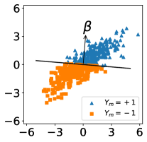
(a)

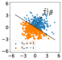
(b)

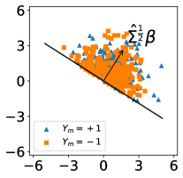
(c)

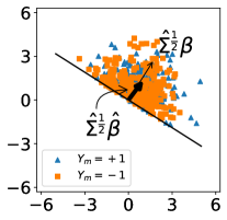
(d)

Figure 1: Intuition behind the estimator in Eq. (3). We consider a dataset of i.i.d. Gaussian samples $\{\bm{X}_{i}\}_{i=1}^{2N}$. Differences $\bm{X}_{I_{m}}-\bm{X}_{J_{m}}$ are shown in Fig. 1(a), along with ${\bm{\beta}}$ and the corresponding separating hyperplane. Colors indicate labels $Y_{m}\in\{-1,+1\}$. We can rewrite Eq. (3) as $\hat{\bm{\beta}}=\bm{\hat{\Sigma}}^{-\frac{1}{2}}\cdot\frac{1}{M}\sum_{m=1}^{M}Y_{m}\hat{\bm{\Sigma}}^{-\frac{1}{2}}(\bm{X}_{I_{m}}-\bm{X}_{J_{m}})$. Multiplying vectors $\bm{X}_{I_{m}}-\bm{X}_{J_{m}}$ with $\hat{\bm{\Sigma}}^{-\frac{1}{2}}$ gives the whitened sample pairs in Fig. 1(b); in this coordinate system, the separating hyperplane has normal $\bm{\hat{\Sigma}}^{\frac{1}{2}}\bm{\beta}$. The resulting whitened pairs are multiplied by the labels $Y_{m}$ in Fig. 1(c); this results in a “mirroring” over the separating hyperplane defined by $\bm{\hat{\Sigma}}^{\frac{1}{2}}\bm{\beta}$. Their average (i.e., $\hat{\bm{\Sigma}}^{\frac{1}{2}}\hat{\bm{\beta}}$) is approximately co-linear with $\bm{\hat{\Sigma}}^{\frac{1}{2}}\bm{\beta}$. The final multiplication with $\hat{\bm{\Sigma}}^{-1/2}$ recovers ${\bm{\beta}}$ (up to a multiplicative constant).

Parameter Estimation. The learner observes $\mathcal{D}$ and estimates $\bm{\beta}$ via:

$$\hat{\bm{\beta}}=\textstyle\frac{1}{M}\sum_{m=1}^{M}Y_{m}{\bm{\hat{\Sigma}}^{-1}}(\bm{X}_{I_{m}}-\bm{X}_{J_{m}})\in\mathbb{R}^{d},$$ (3)

where $\bm{\hat{\Sigma}}$ is an estimator of $\bm{\Sigma}$, computed over the second half of the samples through:

$$\bm{\hat{\Sigma}} =\textstyle\frac{1}{N-d-2}\sum_{i=N+1}^{2N}(\bm{X}_{i}-\bm{\hat{\mu}})(\bm{X}_{i}-\bm{\hat{\mu}})^{\top},\leavevmode\nobreak\ \text{where}\leavevmode\nobreak\ \bm{\hat{\mu}}=\frac{1}{N}\sum_{i=N+1}^{2N}\bm{X}_{i}.$$ (4)

Note that $\mathbb{E}[\bm{\hat{\Sigma}}^{-1}]=\bm{\Sigma}^{-1}$ (see, e.g., [59]). We separate the dataset in two halves to ensure the independence of $\bm{\hat{\Sigma}}$ from labels in $\mathcal{D}$. Eq. (3) resembles a two-class linear discriminant analysis (LDA) estimator (see, e.g., [60]) and is indeed unbiased up to a positive multiplicative constant (see Lemma 7); this is a consequence of Stein’s Lemma [61], stated formally in Section 4. Fig. 1 provides some intuition as to why this is the case. Despite the simplicity of our proposed estimator, characterizing its sampling complexity poses a significant challenge. Non-asymptotic bounds establishing consistency typically rely on i.i.d. assumptions; this is indeed natural to assume for samples $\{\bm{X}_{i}\}_{i=1}^{2N}.$ However, pairwise comparisons introduce correlations in labels $\{\bm{Y}_{m}\}_{m=1}^{M}$: this is precisely because samples are re-used in pairs. We stress that conditioning on $\{\bm{X}_{i}\}_{i=1}^{2N}$ does not resolve this issue, as labels are still dependent through random variables $({I}_{m},{J}_{m})$.

Table 1: Summary of Notation

$N$	number of samples	$\bm{X}_{i}$	Gaussian feature vector
$M$	number of comparisons	$d$	dimensionality of a feature vector
$\left\|\cdot\right\|$	$\ell_{2}$ (spectral) norm of vectors (matrices)	$i,n$	sample index in $[N]$
$Y_{m}$	comparison label	$m$	comparison index in $[M]$
$I_{m},J_{m}$	uniform random variables in $[N]$	$\mathcal{D}$	comparison dataset
$[N]$	set of integers from $1$ to $N$	$\bm{\beta}$	parameter vector/model in $\mathbb{R}^{d}$
$c_{i}$	constants

4 Technical Preliminary

In this section, we review some known results. The first is a variant of Stein’s lemma from Liu [62]; we use this to show that our estimator is unbiased up to a constant.

Lemma 1 (Stein’s Lemma [61, 62]).

Let $\bm{X}\in\mathbb{R}^{d}$, $\bm{X}^{\prime}\in\mathbb{R}^{d^{\prime}}$ be jointly Gaussian random vectors. Let the function $h:\mathbb{R}^{d^{\prime}}\rightarrow\mathbb{R}$ be differentiable almost everywhere and satisfy $\mathbb{E}\left[|\partial h\left(\bm{X}^{\prime}\right)/\partial X_{i}|\right]<\infty$, $i\in[d^{\prime}]$, then $\mathrm{Cov}\left(\bm{X},h(\bm{X}^{\prime})\right)=\mathrm{Cov}\left(\bm{X},\bm{X}^{\prime}\right)\mathbb{E}\left[\nabla h\left(\bm{X}^{\prime}\right)\right]$.

The second lemma we utilize bounds the tail of the norm of standard Gaussian vectors.

Lemma 2 (Centralized Chi-Squared Tail Bound [63]).

Let $F_{X}(x;k)$ be the CDF of centralized chi-square distribution with $k$ degrees of freedom. Then, $1-F_{X}(zk;k)\leq(ze^{1-z})^{k/2}$ for $z>1$.

A consequence of the way we select random pairs is that the joint distribution of the number of times each sample is selected is multinomial. The next inequality provides a bound for such variables:

Lemma 3 (Bretagnolle-Huber-Carolle Inequality [64]).

Let $\{M_{i}\}_{i=1}^{N}$ be multinomially distributed r.v.s with parameters $M$ , $\{p_{i}\}_{i=1}^{N}$. Then $\Pr\left(\sum_{i=1}^{N}\left|\frac{M_{i}}{M}-p_{i}\right|\geq\epsilon\right)\leq 2^{N}e^{-\frac{\epsilon^{2}M}{2}}.$

We also state the following classic inequality:

Lemma 4 (Hoeffding’s Inequality [65]).

Let $X=\frac{1}{N}\sum^{N}_{i=1}X_{i}$, where $a_{i}\leq X_{i}\leq b_{i}$ and $X_{i}$ are independent, and $\mu=\mathbb{E}[X]$. Then $\Pr(|X\!-\!\mu|\!\geq\!\epsilon)\leq 2e^{-2N^{2}\epsilon^{2}/\sum_{i=1}^{N}(b_{i}-a_{i})}$.

Recall that a random variable $X\in\mathbb{R}$ is sub-gaussian if there exists a $c>0$ for all $t\geq 0$ s.t. $\Pr(|X|>t)\leq 2\exp(-t^{2}/c)$. Then, we define the sub-gaussian norm of $X$, denoted by $\left\|X\right\|_{\psi_{2}}$ as $\left\|X\right\|_{\psi_{2}}=\inf\left\{t>0:\mathbb{E}\left[e^{X^{2}/t^{2}}\right]\leq 2\right\}$. Moreover, a random vector $\bm{X}\in\mathbb{R}^{d}$ is called sub-gaussian if one dimensional marginals $\bm{v}^{\top}\bm{X}$ are sub-gaussian for all $\bm{v}\in S^{d-1}$, where $S^{d-1}=\{\bm{x}\in\mathbb{R}^{d}:\left\|\bm{x}\right\|=1\}$. The sub-gaussian norm of $\bm{X}$ is then defined as $\left\|\bm{X}\right\|_{\psi_{2}}=\sup_{\bm{v}\in S^{d-1}}\left\|\bm{v}^{\top}\bm{X}\right\|_{\psi_{2}}$. The next lemma provides lower and upper bounds for the singular values of random design matrices.

Lemma 5 (Theorem 5.39 of Vershynin [66]).

Let $\bm{A}\in\mathbb{R}^{N\times d}$ be a matrix whose rows $\bm{A}_{i}$ are independent sub-gaussian isotropic random vectors. Then for every $t\geq 0$, with probability at least $1-2e^{-ct^{2}}$ one has $\sqrt{N}-C\sqrt{d}-t\leq\lambda_{\min}[\bm{A}]\leq\lambda_{\max}[\bm{A}]\leq\sqrt{N}+C\sqrt{d}+t$ where $c,C>0$ depend only on the maximum sub-gaussian norm $\max_{i}\left\|\bm{A}_{i}\right\|_{\psi_{2}}$ of the rows.

We use Lemma 5 to bound the eigenvalues of the feature covariance matrix. Lastly, the next lemma is used for bounding the norm of sub-gaussian random vectors.

Lemma 6 (Theorem 1 of Hsu et al. [67]).

Let $\bm{A}\in\mathbb{R}^{m\times n}$ be a matrix, and let $\Sigma\equiv\bm{A}^{\top}\bm{A}$. Suppose that $\bm{x}\in\mathbb{R}^{d}$ is a sub-gaussian random vector with mean $\bm{\mu}\in\mathbb{R}^{d}$ and $\sigma=\left\|\bm{x}\right\|_{\psi_{2}}$. For all $t>0$, $\Pr(\left\|\bm{A}\bm{x}\right\|^{2}>\sigma^{2}(\mathrm{Tr}(\Sigma)+2\sqrt{\mathrm{Tr}(\Sigma^{2})t}+2\left\|\Sigma\right\|t)+\left\|\bm{A}\bm{\mu}\right\|^{2}(1+4(\frac{\left\|\Sigma\right\|^{2}}{\mathrm{Tr}(\Sigma^{2})}t)^{1/2}+\frac{4\left\|\Sigma\right\|^{2}}{\mathrm{Tr}(\Sigma^{2})}t)^{1/2})\leq e^{-t}$.

5 Main Results

We first establish that $\bm{\hat{\beta}}$ is an unbiased estimator of $\bm{\beta}$ up to a multiplicative constant.

Lemma 7.

For $\hat{\bm{\beta}}$ in Eq. (3), $\mathbb{E}[\hat{\bm{\beta}}]\!=\!c_{1}\bm{\beta},$ where $c_{1}\!=\!4\mathbb{E}\left[f^{\prime}\left(\bm{\beta}^{T}(\bm{X}_{I_{m}}\!-\!\bm{X}_{J_{m}})\right)\right]\!>\!0$.

The proof can be found in A. This result is a consequence of Stein’s lemma [61] (see Lemma 1 in Section 4). Learning ${\bm{\beta}}$ up to a multiplicative constant suffices, as only the direction is enough to reveal the separating hyperplane between positive and negative sample pairs. Constant $c_{1}$ captures label noise: by (2), $f^{\prime}$ is non-negative and maximized at zero; for functions $f$ that are “flatter” around zero the maximum value of $f^{\prime}$ and, therefore, $c_{1}$ is smaller. Such $f$ also result in noisy labels. Crucially, although our guarantees depend on $c_{1}$ (see Theorem. 1 below), our estimator does not depend on $c_{1}$: no knowledge of $c_{1}$ is required to compute $\hat{\bm{\beta}}$ via Eq. (3). Theorem 1 establishes that the parameters $\bm{\beta}$ are PAC learnable.

Theorem 1.

For $\epsilon>0$, sample count $N/\log^{2}N=\Omega\left(\frac{d}{\epsilon^{2}\lambda_{d}}\right)$ and comparison count $M=\Omega\left(\frac{dN\log^{3}N}{\epsilon^{2}\lambda_{d}}\right)$,

$$\Pr\left(\left\|\hat{\bm{\beta}}-c_{1}\bm{\beta}\right\|\geq\epsilon\right) \leq c_{2}N\max\left\{\left(\frac{\sqrt{6\log N}}{N}\right)^{d},e^{-\frac{N\epsilon^{2}\lambda_{d}}{c_{3}d\log N}}\right\},$$ (5)

where $c_{1}>0$ is given by Lemma 7 and $c_{2},c_{3}>0$ are absolute constants.

Theorem 1, which we prove below, allows us to characterize the sample complexity of $\bm{\hat{\beta}}$ in terms of the ambient dimension $d$, number of samples $N$, and number of comparisons $M$. It implies that to attain an accuracy $\epsilon>0$ with high probability, the estimator requires $\Omega(d\log^{2}N/\epsilon^{2}\lambda_{d})$ samples; this is of the same order as standard PAC learning guarantees for linear classifiers [45, 48, 68] and is also corroborated by our experiments in Section 7. Moreover, the number of comparisons required to attain an accuracy $\epsilon>0$ is $\Omega(dN\log^{3}N/\epsilon^{2}\lambda_{d})$, i.e. comparisons scale almost linearly with $N$.

We emphasize that, to identify the separating plane, it suffices to know $\bm{\beta}$ up to a non-negative multiplicative constant. This motivates the l.h.s. of Eq. (5) in Theorem 1. Nevertheless, the above guarantee should become more stringent for smaller $c_{1}>0$. Recalling that $c_{1}$ captures the level of label noise (smaller indicates more noise), the latter’s impact on this bound is captured by replacing desired accuracy $\epsilon$ with $\epsilon^{\prime}=c_{1}\epsilon$, so that $c_{1}$ appears as an additional constant in the r.h.s. of Eq. (5).

6 Proof of Theorem 1

The proof proceeds in the following manner. We first use a union bound to bound the tail of $\left\|\bm{\hat{\beta}}-c_{1}\bm{\beta}\right\|$ via several constituent terms. Contrary to standard concentration proofs, however, sums appearing in these terms involve dependent random variables. We nevertheless bound these terms by union bounds, conditioning, and leveraging the boundedness of random variables summed. From a technical standpoint, we leverage the Bretagnolle-Huber-Carolle inequality (see Lemma 3), and combine it with classic concentration inequalities (like Hoeffding’s inequality, Lemma 4, and Lemma 16, due to [66]). We start with a simple bound on $\left\|\hat{\bm{\beta}}-c_{1}\bm{\beta}\right\|$.

Lemma 8.

The estimator $\hat{\bm{\beta}}$ given by Eq. (3) satisfies:

$$\Pr\left(\left\|\hat{\bm{\beta}}-c_{1}\bm{\beta}\right\|>\epsilon\right)\leq 4\Pr\left(\left\|\bm{\hat{\Sigma}}^{-1}-\bm{\Sigma}^{-1}\right\|\cdot\left\|\mathbb{E}[Y_{m}(\bm{X}_{I_{m}}-\bm{\mu})]\right\|>\epsilon/6\right)$$

$$+4\Pr\bigg{(}\left\|\frac{1}{M}\!\sum_{m=1}^{M}\!Y_{m}\bm{\Sigma}^{-1/2}(\bm{X}_{I_{m}}\!\!-\!\bm{\mu})\!-\!\mathbb{E}[Y_{m}\bm{\Sigma}^{-1/2}(\bm{X}_{I_{m}}\!\!-\!\bm{\mu})]\right\|\!>\!\frac{\sqrt{\lambda_{d}}\epsilon}{6}\bigg{)}.$$

The proof, via a union bound, can be found in B. The terms $Y_{m}$, $\bm{X}_{I_{m}}-\bm{\mu}$ are not independent. This is because (a) the same sample ${\bm{X}_{i}}$ can be selected more than once, and, crucially, (b) the labels $Y_{m}$ are coupled via the selection of the second sample in each pair. As a consequence, standard concentration bounds do not immediately apply. As a remedy, we condition on events under which the above variables are independent and refine this bound further. To do so, we introduce several quantities of interest. Let

$$\bm{W}_{n}=\bm{\Sigma}^{-1/2}(\bm{X}_{n}-\bm{\mu}),$$ (6)

be the normalized feature vectors. For $n\in[N]$, let the number of times $I_{m}=n$ be

$$M_{n}=\textstyle\sum_{m=1}^{M}\mathbbm{1}_{I_{m}=n}.$$ (7)

For $n,j\in[N]$, let $g_{n,j}:(\mathbb{R}^{d})^{2}\rightarrow[-1,1]$ be the expected comparison label conditioned on the features of samples $n,j\in[N]$ selected in a pair, i.e.:

$$\textstyle g_{n,j}(\bm{x}_{n},\bm{x}_{j}) =\mathbb{E}[Y_{m}|I_{m}=n,J_{m}=j,\{\bm{X}_{n^{\prime}}=\bm{x}_{n^{\prime}}\}_{n^{\prime}=1}^{N}]=2f(\bm{\beta}^{\top}(\bm{x}_{n}-\bm{x}_{j}))-1.$$

Let $g_{n}:\mathbb{R}^{d}\rightarrow[-1,1]$ be the expected label conditioned on the $I_{m}$-th sample:

$$g_{n}(\bm{x}) =\textstyle\mathbb{E}[Y_{m}\mid I_{m}=n,\bm{X}_{n}=\bm{x}]=\int g_{n,1}(\bm{x},\bm{y})\bm{f}_{\bm{X}_{1}}(\bm{y})\bm{d}\bm{y}.$$ (8)

We will also need a similar quantity, $\tilde{g}_{n}:(\mathbb{R}^{d})^{N}\rightarrow[-1,1]$:

$$\tilde{g}_{n}(\{\bm{x}_{n^{\prime}}\}_{n^{\prime}=1}^{N}) =\textstyle\mathbb{E}[Y_{m}\mid I_{m}=n,\{\bm{X}_{n^{\prime}}=\bm{x}_{n^{\prime}}\}_{n^{\prime}=1}^{N}]=\frac{1}{N}\sum_{j=1}^{N}g_{n,j}(\bm{x}_{n},\bm{x}_{j}).$$ (9)

Note that $g_{n}$ and $\tilde{g}_{n}$ are distinct, but the latter can be seen as a quantity that concentrates to $g_{n}$ as $N$ becomes large. We denote by $z_{n}:(\mathbb{R}^{d})^{N}\rightarrow[-2,2]$ their difference, i.e.:

$$\textstyle z_{n}(\{\bm{x}_{n^{\prime}}\}_{n^{\prime}=1}^{N})=\tilde{g}_{n}(\{\bm{x}_{n^{\prime}}\}_{n^{\prime}=1}^{N})-g_{n}(\bm{x}_{n}).$$ (10)

Finally, let $\Delta_{n}\!:\!(\mathbb{R}^{d})^{N}\!\rightarrow\![-2,2]$ be the difference between true label averages and $\tilde{g}_{n}$:

$$\textstyle\Delta_{n}(\{\bm{x}_{n^{\prime}}\}_{n^{\prime}=1}^{N})=\frac{1}{M_{n}}\sum_{m:\leavevmode\nobreak\ I_{m}=n}Y_{m}-\tilde{g}_{n}(\{\bm{x}_{n^{\prime}}\}_{n^{\prime}=1}^{N}).$$ (11)

Our next lemma bounds the second term in the r.h.s. of Lemma 8.

Lemma 9.

For $M_{n},g_{n},\tilde{g}_{n},z_{n},\Delta_{n}$ given by Equations (7), (8), (9), (10), (11),

$$\left\|\frac{1}{M}\sum_{m=1}^{M}Y_{m}\bm{\Sigma}^{-1/2}(\bm{X}_{I_{m}}-\bm{\mu})-\mathbb{E}[Y_{m}\bm{\Sigma}^{-1/2}(\bm{X}_{I_{m}}-\bm{\mu})]\right\|$$

$$\leq\left\|\sum_{n=1}^{N}\left(\frac{M_{n}}{M}-\frac{1}{N}\right)\bm{W}_{n}\tilde{g}_{n}(\{\bm{X}_{n^{\prime}}\}_{n^{\prime}=1}^{N})\right\|+\left\|\frac{1}{M}\sum_{n=1}^{N}\bm{W}_{n}M_{n}\Delta_{n}(\{\bm{X}_{n^{\prime}}\}_{n^{\prime}=1}^{N})\right\|$$

$$+\left\|\frac{1}{N}\sum_{n=1}^{N}\bm{W}_{n}z_{n}(\{\bm{X}_{n^{\prime}}\}_{n^{\prime}=1}^{N})\right\|+\left\|\frac{1}{N}\sum_{n=1}^{N}\bm{W}_{n}g_{n}(\bm{X}_{n})\!-\!\mathbb{E}[Y_{m}\bm{\Sigma}^{-1/2}(\bm{X}_{I_{m}}\!-\!\bm{\mu})]\right\|.$$

The proof can be found in C. The four terms in the r.h.s. are bounded individually in the rest of the proof. We bound the first term in Lemma 9 with Lemma 10.

Lemma 10.

For all $\delta_{0}>d$,

$$\Pr\bigg{(}\left\|\sum_{n=1}^{N}\left(\frac{M_{n}}{M}-\frac{1}{N}\right)\bm{W}_{n}\tilde{g}_{n}(\{\bm{X}_{n^{\prime}}\}_{n^{\prime}=1}^{N})\right\|\!>\!\epsilon\bigg{)}\!\leq\!N\left(\frac{\delta_{0}}{d}e^{1-\frac{\delta_{0}}{d}}\right)^{d/2}\!+\!2^{N}e^{-\frac{\epsilon^{2}M}{2\delta_{0}}}.$$

The proof can be found in D. We rely on the fact that $|\tilde{g}_{n}|\leq 1$, as well as (a) the norm $\left\|\bm{W}_{n}\right\|$ can be bounded by a centralized Chi-Squared tail bound, while (b) the quantity $|\frac{M_{n}}{M}-\frac{1}{N}|$ can be bounded by the Bretagnolle-Huber-Carol Inequality (see Lemma 3 in Section 4). Next, we bound the second term in Lemma 9.

Lemma 11.

For all $\delta_{1}<\frac{\epsilon^{2}}{4d}$ and $\delta_{2}>d$,

$$\Pr\bigg{(}\left\|\frac{1}{M}\sum_{n=1}^{N}\bm{W}_{n}M_{n}\Delta_{n}\{\bm{X}_{n^{\prime}}\}_{n^{\prime}=1}^{N}\right\|\!>\!\epsilon\bigg{)}\leq N\left(\frac{\epsilon^{2}}{4d\delta_{1}}e^{1-\frac{\epsilon^{2}}{4d\delta_{1}}}\right)^{d/2}$$

$$+N\left(\frac{\delta_{2}}{d}e^{1-\frac{\delta_{2}}{d}}\right)^{d/2}+2^{N}e^{-\frac{\epsilon^{2}M}{8\delta_{1}\delta_{2}}}+2e^{\log N-\frac{M\delta_{1}}{2N}-o(\frac{M\delta_{1}}{2N})}.$$

The proof is in E. We bound individual terms, $\left\|\bm{W}_{n}\right\|$, $|\Delta_{n}|$, $\big{|}\frac{M_{n}}{M}-\frac{1}{N}\big{|}$ respectively using a centralized Chi-Squared tail bound, Hoeffding’s inequality, and the moment generating function of the binomial distribution. Our next lemma bounds the third term in Lemma 9:

Lemma 12.

For all $\delta_{3}\leq\epsilon^{2}/d$,

$$\Pr\bigg{(}\left\|\frac{1}{N}\sum_{n=1}^{N}\bm{W}_{n}z_{n}(\{\bm{X}_{n^{\prime}}\}_{n^{\prime}=1}^{N})\right\|>\epsilon\bigg{)}\leq N\left(\frac{\epsilon^{2}}{d\delta_{3}}e^{1-\frac{\epsilon^{2}}{d\delta_{3}}}\right)^{d/2}+2Ne^{-\frac{N\delta_{3}}{2}}.$$

The proof can be found in F. We bound terms $\left\|\bm{W}_{n}\right\|$ and $|z_{n}|$ individually. For the former, we again use a centralized Chi-Squared tail bound. For the latter, we indeed show that, for large sample sizes $N$, $\tilde{g}_{n}$ concentrates around $g_{n}$ using Hoeffding’s inequality. We bound the last term in Lemma 9 as follows:

Lemma 13.

For an absolute constant $c_{2}>0$,

$$\Pr\!\bigg{(}\!\left\|\frac{1}{N}\!\sum_{n=1}^{N}\!\bm{W}_{n}g_{n}(\bm{X}_{n})\!-\!\mathbb{E}[Y_{m}\bm{\Sigma}^{-1/2}(\bm{X}_{I_{m}}\!-\!\bm{\mu})]\right\|\!>\!\epsilon\!\bigg{)}\!\leq\!e^{-\frac{1}{4}\left(\sqrt{\frac{N\epsilon^{2}}{c_{2}}-d}-\sqrt{d}\right)^{2}}.$$

The proof, which is in G, shows that individual terms are sub-gaussian and uses a concentration bound due to Hsu et al. [67]. The second term in Lemma 8 is bounded as follows:

Lemma 14.

For the estimator $\bm{\hat{\Sigma}}$ given by Eq. (4), and for $\sqrt{N}\!>\!\sqrt{\frac{N-d-2}{\frac{\lambda_{d}}{d\sqrt{2\lambda_{1}}}\epsilon+1}}\!+\!c_{3}\!\sqrt{d}$ where $c_{3},c_{4}>0$ are absolute constants,

$$\Pr\left(\left\|\bm{\hat{\Sigma}}^{-1}-\bm{\Sigma}^{-1}\right\|\cdot\left\|\mathbb{E}[Y_{m}(\bm{X}_{I_{m}}-\bm{\mu})]\right\|>\epsilon\right) \leq 2e^{-c_{4}\big{(}\sqrt{N}-\sqrt{\frac{N-d-2}{\frac{\lambda_{d}}{d\sqrt{2\lambda_{1}}}\epsilon+1}}-c_{3}\sqrt{d}\big{)}^{2}}.$$

The proof can be found in H. We use a concentration bound on the minimum singular value of the design matrix due to Vershynin [66]. Combining Lemmas 8, 9, 10, 11, 12, 13 and 14 via a union bound gives:

$$\Pr\left(\left\|\hat{\bm{\beta}}-c_{1}\bm{\beta}\right\|\geq\epsilon\right) \leq 8e^{-c_{4}\bigg{(}\sqrt{N}-\sqrt{\frac{N-d-2}{\frac{\lambda_{d}}{6d\sqrt{2\lambda_{1}}}\epsilon+1}}-c_{3}\sqrt{d}\bigg{)}^{2}}+4e^{-\frac{1}{4}\left(\sqrt{\frac{\epsilon^{2}N\lambda_{d}}{c_{2}}-d}-\sqrt{d}\right)^{2}}$$

$$+2^{N+2}e^{-\frac{\epsilon^{2}M\lambda_{d}}{4608\delta_{1}\delta_{2}}}+8e^{\log N-\frac{M\delta_{1}}{2N}-o\left(\frac{M\delta_{1}}{2N}\right)}+8Ne^{-\frac{N\delta_{3}}{2}}$$

$$+4N\left(\frac{\epsilon^{2}\lambda_{d}}{2304d\delta_{1}}e^{1-\frac{\epsilon^{2}\lambda_{d}}{2304d\delta_{1}}}\right)^{d/2}+4N\left(\frac{\epsilon^{2}\lambda_{d}}{576d\delta_{3}}e^{1-\frac{\epsilon^{2}\lambda_{d}}{576d\delta_{3}}}\right)^{d/2}$$

$$+2^{N+2}e^{-\frac{\epsilon^{2}M\lambda_{d}}{1152\delta_{0}}}+4N\left(\frac{\delta_{0}}{d}e^{1-\frac{\delta_{0}}{d}}\right)^{d/2}+4N\left(\frac{\delta_{2}}{d}e^{1-\frac{\delta_{2}}{d}}\right)^{d/2}.$$

Setting $M=\Omega(\frac{dN\log^{3}N}{\lambda_{d}\epsilon^{2}})$, $\delta_{0}=d\log^{2}N$, $\delta_{1}=4\lambda_{d}\epsilon^{2}/d\log^{2}N$, $\delta_{2}=d\log^{2}N$ and $\delta_{3}=\epsilon^{2}\lambda_{d}/1152d\log N$, the bound reduces to $\Pr\left(\left\|\hat{\bm{\beta}}-c_{1}\bm{\beta}\right\|\geq\epsilon\right)\leq c_{6}N$ $\max\left\{\left(\frac{\sqrt{6\log N}}{N}\right)^{d},e^{-\frac{N\epsilon^{2}\lambda_{d}}{c_{7}d\log N}}\right\}$ for $N>\frac{c_{8}d\log^{2}N}{\epsilon^{2}\lambda_{d}},$ where $c_{6},c_{7},c_{8}>0$ are absolute constants. We derive this in I. ∎

7 Experiments

Synthetic Experiment Setup. To support our theoretical findings, we evaluate the estimator given by Eq. (3) with a synthetic dataset as follows: We sample the true parameter $\bm{\beta}\in\mathbb{R}^{d}$ from $\mathcal{N}(\bm{0},10\bm{I})$. We sample $\bm{\mu}\in\mathbb{R}^{d}$ uniformly at random from $[-5,5]^{d}$. To assess the impact of minimum eigenvalue of $\bm{\Sigma}\in\mathbb{R}^{d\times d}$ on estimator accuracy, we generate $\bm{\Sigma}$ as follows. We generate a random orthonormal basis of $\mathbb{R}^{d}$, and choose a smallest eigenvalue $\lambda_{d}\in(0,1]$. We then a construct $\bm{\Sigma}$ whose eigenvectors are the selected orthonormal basis, and $d$ eigenvalues equidistributed in $[\lambda_{d},1]$. We treat $\lambda_{d}$ as a tunable parameter. Each feature vector $\bm{x}_{i}\in\mathbb{R}^{d},i\in[2N]$, is independently sampled from $\mathcal{N}(\bm{\mu},\bm{\Sigma})$. We sample pairs $(I_{m},J_{m}),m\in[M]$, uniformly at random from $[N]\times[N]$. Noisy labels $Y_{m}$ are sampled using Eq. (1) where $f(x)=(1+e^{-\alpha x})^{-1}$ and $0\!<\!\alpha\!<\!\infty$. By adjusting $\alpha$, we choose the fraction $p_{e}\in[0,1]$ of $M$ comparisons that are flipped, i.e. are incorrect. We repeat all experiments with 10 random generations of parameters $\bm{\beta}$, $\bm{\mu}$, $\bm{\Sigma}$. We estimate quantities $c_{1}$ and $p_{e}$ numerically (see J).

Metrics. We measure the performance of the estimator $\hat{\bm{\beta}}$ with two metrics. The first error metric is $\left\|\bm{\hat{\beta}}-c_{1}\bm{\beta}\right\|$. The second metric is

$$\angle(\bm{\hat{\beta}},\bm{\beta})=\cos^{-1}{(\bm{\hat{\beta}}^{\top}\bm{\beta}/||\bm{\hat{\beta}}||||\bm{\beta}||)},$$ (12)

i.e., the angle between $\bm{\hat{\beta}}$ and $\bm{\beta}$. We report both the average and standard deviation across different random generations.

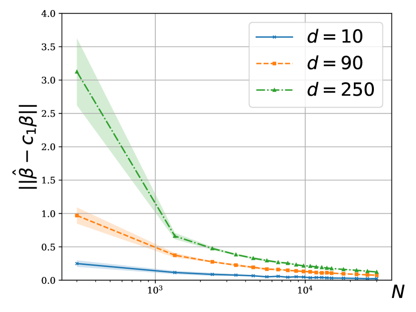
(a) $\lambda_{d}=1,p_{e}=0.2$

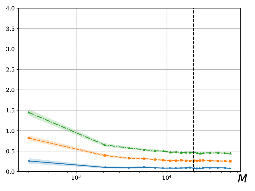
(b) $\lambda_{d}=1,p_{e}=0.2$

Figure 2: (a) The error of the estimator given by Eq. (3) indeed reduces as $N$ increases when $M=\lceil N\log N\rceil$ and we see that the estimator is converging to $c_{1}\bm{\beta}$. (b) The error reduces when $M$ increases while $N$ is kept constant, however the decay is insignificant after $M=N\log N$, which is denoted with the black dashed line. This agrees with our theory that $M=\tilde{\Omega}(N)$. The shaded area is the standard deviation.

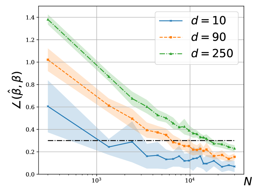
(a) $p_{e}=0$

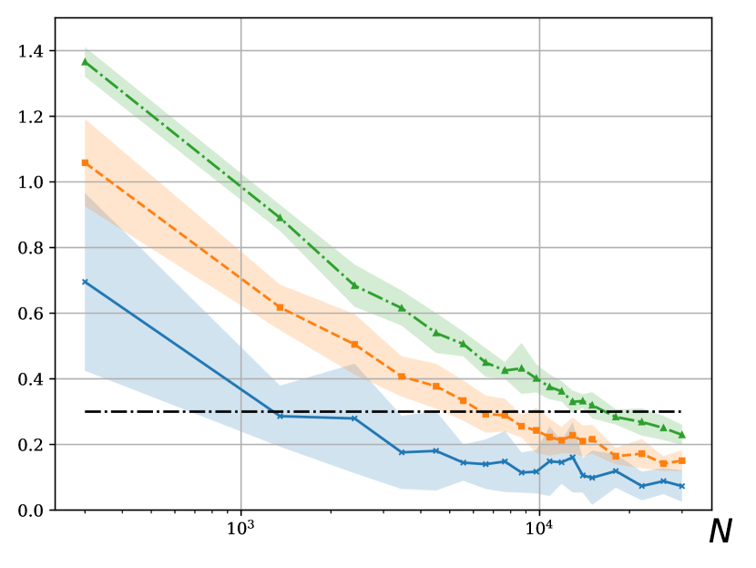
(b) $p_{e}=0.2$

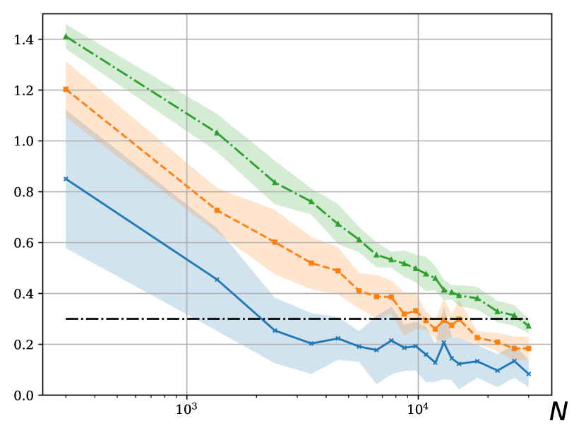
(c) $p_{e}=0.4$

Figure 3: The angle between the true parameter $\bm{\beta}$ and the estimator $\bm{\hat{\beta}}$, plotted against $N$ for different error probabilities $p_{e}$ when $M=\lceil N\log N\rceil$ and $\lambda_{d}=1/200$. (a) The noiseless case. (b) The case where $20\%$ of the labels are flipped. (c) The case where $40\%$ of the labels are flipped. Even though noise increases error, increasing $N$ allows the estimator to reduce the error arbitrarily. This shows that the estimator $\bm{\hat{\beta}}$ is able to recover the direction of the true parameter $\bm{\beta}$ as $N$ increases. The shaded area is the standard deviation.

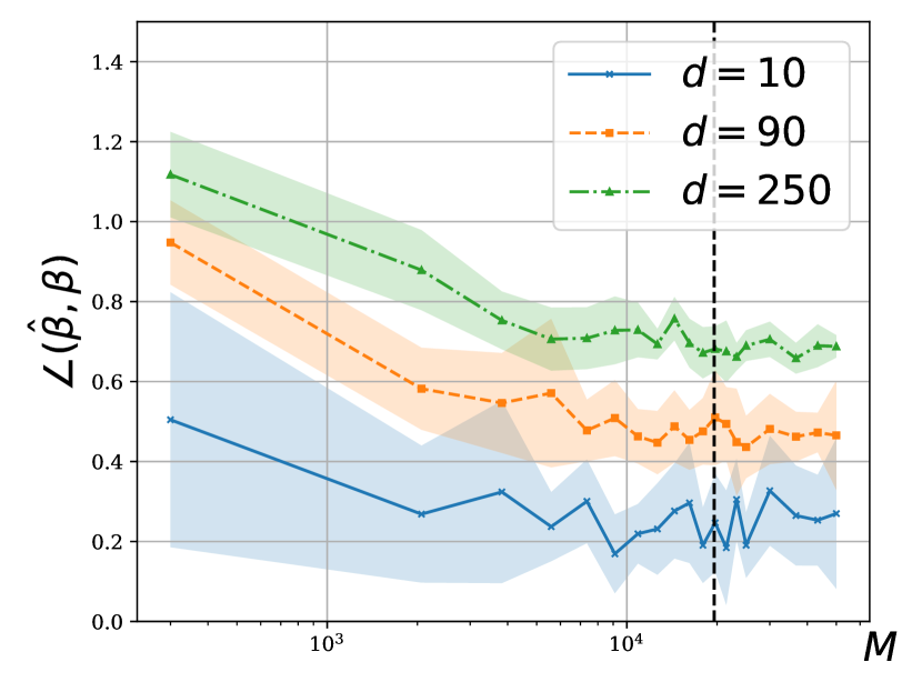
(a) $p_{e}=0$

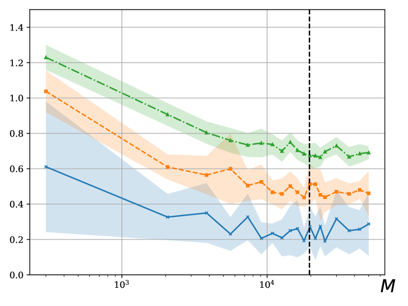
(b) $p_{e}=0.2$

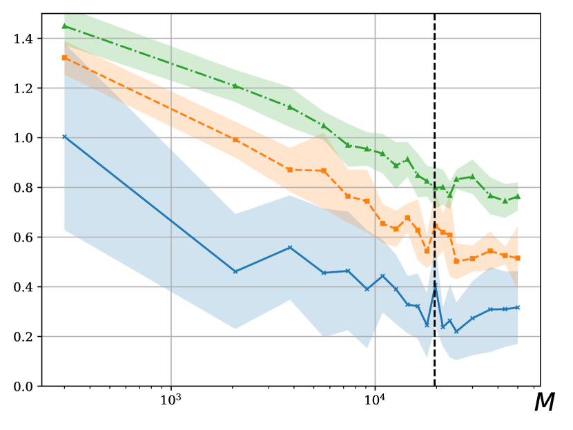
(c) $p_{e}=0.4$

Figure 4: The angle between the true parameter $\bm{\beta}$ and the estimator $\bm{\hat{\beta}}$, plotted against $M$ for different error probabilities $p_{e}$ when $N=2.5\times 10^{3}$ and $\lambda_{d}=1/200$. (a) The noiseless case. (b) The case where $20\%$ of the labels are flipped. (c) The case where $40\%$ of the labels are flipped. Increasing $M$ reduces the error for all $p_{e}$ values. However, once $M=N\log N$ which is denoted with the black dashed line, the reduction is insignificant. This is due to the fact that a higher $N$ is required for smaller $\epsilon$ as $N=\Omega(d/\lambda_{d}\epsilon^{2})$, i.e. $N$ needs to scale inversely quadratic with $\epsilon$. This supports our theory that the estimator $\bm{\hat{\beta}}$ does better as $M$ increases; however, for arbitrarily small $\epsilon$, $N$ needs to increase too. The shaded area is the standard deviation.

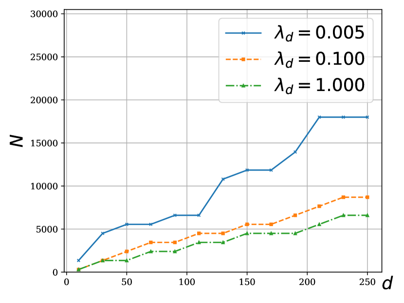
(a) $p_{e}=0$

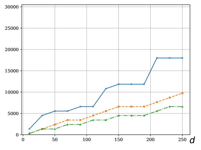
(b) $p_{e}=0.2$

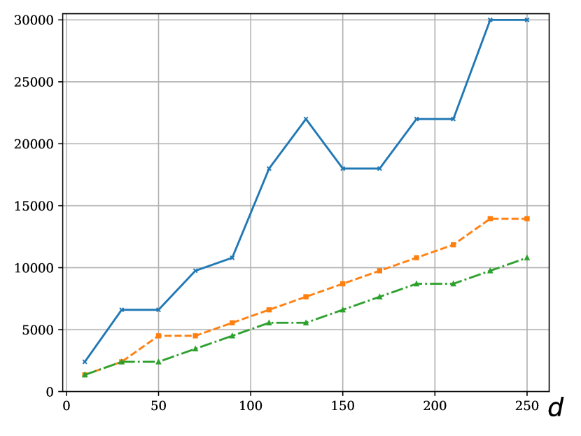
(c) $p_{e}=0.4$

Figure 5: Minimum $N$ that achieves $\angle(\bm{\hat{\beta}},\bm{\beta})\leq 0.3$ plotted against dimensionality $d$ for different values of the minimum eigenvalue $\lambda_{d}$ of the feature covariance and error probabilities $p_{e}$. (a) The noiseless case. (b) The case where $20\%$ of the labels are flipped. (c) The case where $40\%$ of the labels are flipped. As the probability of error and the condition number of the feature covariance increases, we require more samples. Crucially, we observe the linear dependence of $N$ to $d$ and this supports that $N=\Omega(d/\lambda_{d}\epsilon^{2})$.

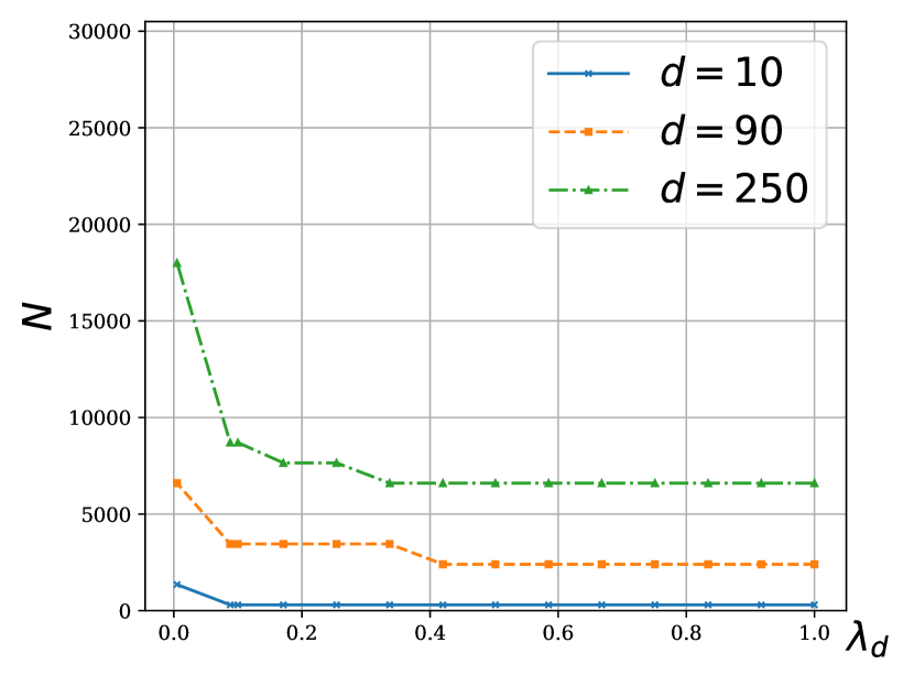
(a) $p_{e}=0$

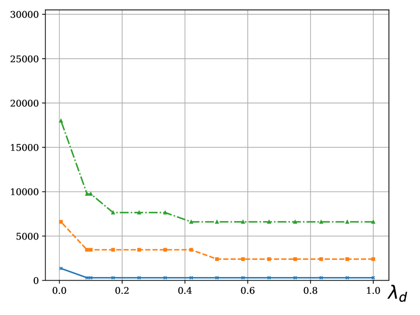
(b) $p_{e}=0.2$

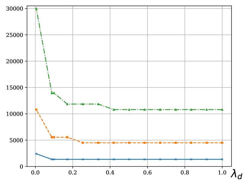
(c) $p_{e}=0.4$

Figure 6: Minimum $N$ that achieves $\angle(\bm{\hat{\beta}},\bm{\beta})\leq 0.3$ plotted against the minimum eigenvalue $\lambda_{d}$ of the feature covariance for different dimensionality $d$ and probability of error $p_{e}$. (a) The noiseless case. (b) The case where $20\%$ of the labels are flipped. (c) The case where $40\%$ of the labels are flipped. We observe that increasing error increases the required $N$ and the inversely proportional dependence of $N$ to $\lambda_{d}$ is observed.

Convergence. In order to investigate the convergence of $\bm{\hat{\beta}}$, we vary the number of samples $N$ in $[300,3\times 10^{4}]$, dimensionality $d\in\{10,90,250\}$ while we set $M=\lceil N\log N\rceil$, and $\lambda_{d}=1$. We select $\alpha$ so that $p_{e}=0.2$. In Fig. 2(a), we plot the error $\left\|\bm{\hat{\beta}}-c_{1}\bm{\beta}\right\|$ as a function of the dataset size $N$. We observe that for each $d$, the error decreases as $N$ increases and $\bm{\hat{\beta}}$ indeed converges to $c_{1}\bm{\beta}$. In Fig. 2(b), we vary $M$ in $[300,5\times 10^{4}]$ and $d\in\{10,90,250\}$ while we set $N=2.5\times 10^{3}$. We observe that increasing $M$ reduces the error. However, the reduction in error is insignificant after $M=N\log N$, which is denoted with the black dashed line in Fig. 2(b). This is consistent with the bound in Theorem 1, which anticipates that $M$ is polylogarithmic in $N$.

Dependence on $N$. We investigate the required number of samples $N$ to attain $\angle(\hat{\bm{\beta}},\bm{\beta})=0.3$. For each $d\in\{10,90,250\}$ and $p_{e}\in\{0,0.2,0.4\}$ we vary $N\in[300,3\times 10^{4}]$, setting $M=\lceil{N\log N}\rceil$, and $\lambda_{d}=1/200$. In Fig. 3, we plot the error $\angle(\bm{\hat{\beta}},\bm{\beta})$ versus the dataset size $N$ under different noise levels $p_{e}$. We observe that as $N$ increases, $\bm{\hat{\beta}}$ indeed achieves $\angle(\hat{\bm{\beta}},\bm{\beta})=0.3$ for all $d$, while the error increase with $d$. This implies that irrespective of the noise level and the corresponding $c_{1}$ value, the estimator $\bm{\hat{\beta}}$ is able to recover the direction of $\bm{\beta}$ as $N$ increases.

Dependence on $M$. We repeat our experiments on the impact of $M$, this time focusing on the angle metric and varying $p_{e}$. We fix $N=2.5\times 10^{3}$, $\lambda_{d}=1/200$ and vary $M\in[300,5\times 10^{4}]$, $d\in\{10,90,250\}$, and $p_{e}\in\{0,0.2,0.4\}$. Fig. 4 plots $\angle(\bm{\hat{\beta}},\bm{\beta})$ versus $M$ under different noise levels. These plots show that the benefit of increasing $M$ again diminishes beyond $M=N\log N$ for all $p_{e}\in\{0,0.2,0.4\}$, represented by the dashed black line. This is again consistent with Theorem 1.

Dependence on $d$. In Fig. 5, we plot the smallest $N$ that achieves $\angle(\hat{\bm{\beta}},\bm{\beta})\leq 0.3$ while we vary $d\in[10,250]$, $\lambda_{d}\in\{1/200,0.1,1\}$ and $p_{e}\in\{0,0.2,0.4\}$. We observe that the required $N$ increases linearly in $d$. This is consistent with the linear dependence of $N$ on $d$ anticipated by Theorem 1.

Dependence on $\lambda_{d}$. In Fig. 6, we investigate the effect of $\lambda_{d}$ on the smallest $N$ that achieves $\angle(\hat{\bm{\beta}},\bm{\beta})\leq 0.3$ for each $p_{e}\in\{0,0.2,0.4\}$ and $d\in\{10,90,250\}$. We observe the inversely proportional relationship between $\lambda_{d}$ and $N$, which is consistent with the $N=\Omega(d/\lambda_{d}\epsilon^{2})$ requirement implied by Theorem 1.

8 Conclusion

Our results suggest that learning parameters of a linear preference model from comparisons can come with guarantees, despite the lack of independence between comparisons. Though our bound on $N$ is tight (as the number of samples cannot be lower than $d$), our experimental results suggest that the bound on $M$ could be sharpened; lower bounds on this quantity also remain open. Given the practical benefit of learning from comparisons over datasets with small samples, understanding the inherent trade-offs between samples, comparisons, and label variance is a very interesting direction to explore. In particular, determining regimes in which learning from comparisons outperforms learning from categorical labels is an important question; our work can serve as a starting point for exploring this formally.

References

Biographies

Berkan Kadıoğlu is a PhD candidate at the Department of Electrical and Computer Engineering, Northeastern University, Boston, MA, since 2017. He received his B.Sc. (2017) in Electrical and Electronics Engineering from Bilkent University, Ankara, Turkey. His research interests include machine learning, statistical learning, deep learning with a focus on learning from comparisons.

Dr. Peng Tian is a postdoctoral research associate at Northeastern University, Boston, MA. He received his Ph.D. and M.S. degree of Electrical Engineering in 2020 and 2017 respectively, from Northeastern University, Boston, MA. He obtained his B.E. degree of Optoelectronic Information Engineering in 2015 from Huazhong University of Science & and Technology, Wuhan, China. His research instests span learning from comparisons, deep learning and AI for healthcare.

Dr. Jennifer G. Dy is a professor at the Department of Electrical and Computer Engineering, Northeastern University, Boston, MA, since 2002. She obtained her MS and PhD in 1997 and 2001 respectively from the School of Electrical and Computer Engineering, Purdue University, West Lafayette, IN, and her BS degree in 1993 from the Department of Electrical Engineering, University of the Philippines. She received an NSF Career award in 2004. She is an editorial board member for the journal, Machine Learning since 2004, publications chair for the International Conference on Machine Learning in 2004, and program committee member for ICML, ACM SIGKDD, AAAI, and SIAM SDM. Her research interests include Machine Learning, Data Mining, Statistical Pattern Recognition, and Computer Vision.

Dr. Deniz Erdoğmus graduated with B.S. in Electrical & Electronics Engineering (EEE), and the B.S. in Mathematics in 1997, and M.S. in EEE in 1999 from the Middle East Technical University, Ankara, Turkey. He received his Ph.D. in Electrical & Computer Engineering from the University of Florida in 2002, where he stayed as a postdoctoral research associate until 2004. Prior to joining the Northeastern faculty in 2008, he held an Assistant Professor position at the Oregon Health and Science University. His expertise is in information theoretic and nonparametric machine learning and adaptive signal processing, specifically focusing on cognitive signal processing including brain interfaces and assistive technologies. Deniz has been serving as an associate editor IEEE Transactions on Signal Processing, Transactions on Neural Networks, Signal Processing Letters, and Elsevier Neurocomputing. He is a member of the IEEE-SPS Machine Learning for Signal Processing Technical Committee.

Dr. Stratis Ioannidis is an associate professor in the Electrical and Computer Engineering Department of Northeastern University, in Boston, MA, where he also holds a courtesy appointment with the College of Computer and Information Science. He received his B.Sc. (2002) in Electrical and Computer Engineering from the National Technical University of Athens, Greece, and his M.Sc. (2004) and Ph.D. (2009) in Computer Science from the University of Toronto, Canada. Prior to joining Northeastern, he was a research scientist at the Technicolor research centers in Paris, France, and Palo Alto, CA, as well as at Yahoo Labs in Sunnyvale, CA. He is the recipient of an NSF CAREER Award, a Google Faculty Research Award, a Facebook Research Award, a Martin W. Essigmann Outstanding Teaching Award, and several best paper awards. His research interests span machine learning, distributed systems, networking, optimization, and privacy.

Appendix A Proof of Lemma 7

The expected value of the estimator is

$$\mathbb{E}[\hat{\bm{\beta}}] =\mathbb{E}\left[\frac{1}{M}\sum_{m=1}^{M}Y_{m}\bm{\hat{\Sigma}}^{-1}(\bm{X}_{I_{m}}-\bm{X}_{J_{m}})\right]\leavevmode\nobreak\ \leavevmode\nobreak\ \leavevmode\nobreak\ \text{by Eq.\eqref{eq:estimator},}$$

$$=\mathbb{E}\left[Y_{m}\bm{\hat{\Sigma}}^{-1}(\bm{X}_{I_{m}}-\bm{X}_{J_{m}})\right]$$

$$=\mathbb{E}\left[\bm{\hat{\Sigma}}^{-1}\right]\mathbb{E}\left[Y_{m}(\bm{X}_{I_{m}}-\bm{X}_{J_{m}})\right]\leavevmode\nobreak\ \leavevmode\nobreak\ \leavevmode\nobreak\ \text{by $\bm{\hat{\Sigma}}^{-1}\mathchoice{\mathrel{\hbox to0.0pt{$\displaystyle\perp$\hss}\mkern 2.0mu{\displaystyle\perp}}}{\mathrel{\hbox to0.0pt{$\textstyle\perp$\hss}\mkern 2.0mu{\textstyle\perp}}}{\mathrel{\hbox to0.0pt{$\scriptstyle\perp$\hss}\mkern 2.0mu{\scriptstyle\perp}}}{\mathrel{\hbox to0.0pt{$\scriptscriptstyle\perp$\hss}\mkern 2.0mu{\scriptscriptstyle\perp}}}Y_{m},\bm{X}_{I_{m}},\bm{X}_{J_{m}}$,}$$

$$=\bm{\Sigma}^{-1}\mathbb{E}\left[Y_{m}(\bm{X}_{I_{m}}-\bm{X}_{J_{m}})\right]\leavevmode\nobreak\ \leavevmode\nobreak\ \leavevmode\nobreak\ \text{by \cite[cite]{[\@@bibref{Number}{hartlap2007your}{}{}]},}$$

$$=\bm{\Sigma}^{-1}\mathbb{E}\left[(\bm{X}_{I_{m}}-\bm{X}_{J_{m}})\mathbb{E}\left[Y_{m}|\bm{X}_{I_{m}}-\bm{X}_{J_{m}}\right]\right]$$

$$=\bm{\Sigma}^{-1}\mathbb{E}\left[(\bm{X}_{I_{m}}-\bm{X}_{J_{m}})\left(2f\big{(}\bm{\beta}^{\top}(\bm{X}_{I_{m}}-\bm{X}_{J_{m}})\big{)}-1\right)\right]$$

$$=\bm{\Sigma}^{-1}\text{Cov}\left[\bm{X}_{I_{m}}-\bm{X}_{J_{m}},2f\left(\bm{\beta}^{T}(\bm{X}_{I_{m}}-\bm{X}_{J_{m}})\right)-1\right]$$

$$=2\bm{\Sigma}^{-1}\text{Cov}\left[\bm{X}_{I_{m}}\!-\!\bm{X}_{J_{m}},\bm{\beta}^{T}(\bm{X}_{I_{m}}\!-\!\bm{X}_{J_{m}})\right]\mathbb{E}\left[f^{\prime}\left(\bm{\beta}^{T}(\bm{X}_{I_{m}}\!-\!\bm{X}_{J_{m}})\right)\right]$$

$$=2\bm{\Sigma}^{-1}\mathbb{E}\left[(\bm{X}_{I_{m}}-\bm{X}_{J_{m}})(\bm{X}_{I_{m}}-\bm{X}_{J_{m}})^{T}\right]\mathbb{E}\left[f^{\prime}\left(\bm{\beta}^{T}(\bm{X}_{I_{m}}-\bm{X}_{J_{m}})\right)\right]\bm{\beta}$$

$$=4\bm{\Sigma}^{-1}\bm{\Sigma}\mathbb{E}\left[f^{\prime}\left(\bm{\beta}^{T}(\bm{X}_{I_{m}}-\bm{X}_{J_{m}})\right)\right]\bm{\beta}=4\mathbb{E}\left[f^{\prime}\left(\bm{\beta}^{T}(\bm{X}_{I_{m}}-\bm{X}_{J_{m}})\right)\right]\bm{\beta}$$

$$=c_{1}\bm{\beta},$$

where the fourth to last line is by Lemma 1 and $c_{1}=4\mathbb{E}\left[f^{\prime}\left(\bm{\beta}^{T}(\bm{X}_{I_{m}}-\bm{X}_{J_{m}})\right)\right]$. Note that $c_{1}$ is strictly positive as $f(x)$ is non-decreasing, and has limits $\lim_{x\rightarrow\infty}f(x)=1$, $\lim_{x\rightarrow-\infty}f(x)=0$. Therefore, there exists an $s\in\mathbb{R}$ at which $f^{\prime}(s)>0$. By continuity, $f^{\prime}(x)$ is therefore strictly positive in an interval around $s$. As a result, the integral in the expectation which defines $c_{1}$ is strictly positive. ∎

Appendix B Proof of Lemma 8

We start by dividing the error into two symmetric terms. We have

$$\left\|\hat{\bm{\beta}}-c\bm{\beta}\right\| =\left\|\frac{1}{M}\sum_{m=1}^{M}Y_{m}\bm{\hat{\Sigma}}^{-1}(\bm{X}_{I_{m}}-\bm{X}_{J_{m}})-\mathbb{E}[Y_{m}\bm{\Sigma}^{-1}(\bm{X}_{I_{m}}-\bm{X}_{J_{m}})]\right\|$$

$$=\Bigg{\|}\frac{1}{M}\sum_{m=1}^{M}Y_{m}\bm{\hat{\Sigma}}^{-1}(\bm{X}_{I_{m}}-\bm{\mu})-\frac{1}{M}\sum_{m=1}^{M}Y_{m}\bm{\hat{\Sigma}}^{-1}(\bm{X}_{J_{m}}-\bm{\mu})$$

$$-\mathbb{E}[Y_{m}\bm{\Sigma}^{-1}\bm{(}X_{I_{m}}-\bm{\mu})]+\mathbb{E}[Y_{m}\bm{\Sigma}^{-1}(\bm{X}_{J_{m}}-\bm{\mu})]\Bigg{\|}$$

$$\leq\left\|\frac{1}{M}\sum_{m=1}^{M}Y_{m}\bm{\hat{\Sigma}}^{-1}(\bm{X}_{I_{m}}-\bm{\mu})-\mathbb{E}[Y_{m}\bm{\Sigma}^{-1}(\bm{X}_{I_{m}}-\bm{\mu})]\right\|$$

$$+\left\|\frac{1}{M}\sum_{m=1}^{M}Y_{m}\bm{\hat{\Sigma}}^{-1}(\bm{X}_{J_{m}}-\bm{\mu})-\mathbb{E}[Y_{m}\bm{\Sigma}^{-1}(\bm{X}_{J_{m}}-\bm{\mu})]\right\|,$$

where the last line is by a triangle inequality and the first line is by Eq. (3) and Lemma 7. Then, we show that these terms are bounded by the same probability. We start by defining $Y_{m}^{\prime}=-Y_{m}$ and note that

$$\Pr(Y_{m}^{\prime}\mid\bm{X}_{I_{m}}=x,\bm{X}_{J_{m}}=y) =\Pr(-Y_{m}\mid\bm{X}_{I_{m}}=x,\bm{X}_{J_{m}}=y)$$

$$=1-f(\bm{\beta}^{\top}(x-y))\leavevmode\nobreak\ \leavevmode\nobreak\ \leavevmode\nobreak\ \text{by Eq.\leavevmode\nobreak\ \eqref{eq:conditional},}$$

$$=f(\bm{\beta}^{\top}(y-x))\leavevmode\nobreak\ \leavevmode\nobreak\ \leavevmode\nobreak\ \text{by Eq.\leavevmode\nobreak\ \eqref{eq:properties}.}$$ (13)

Then, we have

$$\Pr\left(\left\|\frac{1}{M}\sum_{m=1}^{M}Y_{m}\bm{\hat{\Sigma}}^{-1}(\bm{X}_{J_{m}}-\bm{\mu})-\mathbb{E}[Y_{m}\bm{\Sigma}^{-1}(\bm{X}_{J_{m}}-\bm{\mu})]\right\|>\epsilon\right)$$

$$=\Pr\left(\left\|\frac{1}{M}\sum_{m=1}^{M}-Y_{m}\bm{\hat{\Sigma}}^{-1}(\bm{X}_{J_{m}}-\bm{\mu})-\mathbb{E}[-Y_{m}\bm{\Sigma}^{-1}(\bm{X}_{J_{m}}-\bm{\mu})]\right\|>\epsilon\right)$$

$$=\Pr\left(\left\|\frac{1}{M}\sum_{m=1}^{M}Y_{m}^{\prime}\bm{\hat{\Sigma}}^{-1}(\bm{X}_{J_{m}}-\bm{\mu})-\mathbb{E}[Y_{m}^{\prime}\bm{\Sigma}^{-1}(\bm{X}_{J_{m}}-\bm{\mu})]\right\|>\epsilon\right)$$

$$=\Pr\left(\left\|\frac{1}{M}\sum_{m=1}^{M}Y_{m}\bm{\hat{\Sigma}}^{-1}(\bm{X}_{I_{m}}-\bm{\mu})-\mathbb{E}[Y_{m}\bm{\Sigma}^{-1}(\bm{X}_{I_{m}}-\bm{\mu})]\right\|>\epsilon\right),$$ (14)

where the last line is by Eq. (B). We use this result to show that

$$\Pr\left(\left\|\hat{\bm{\beta}}-c\bm{\beta}\right\|>\epsilon\right)\leq\Pr\Bigg{(}\left\|\frac{1}{M}\sum_{m=1}^{M}Y_{m}\bm{\hat{\Sigma}}^{-1}(\bm{X}_{I_{m}}-\bm{\mu})-\mathbb{E}[Y_{m}\bm{\Sigma}^{-1}(\bm{X}_{I_{m}}-\bm{\mu})]\right\|$$

$$+\left\|\frac{1}{M}\sum_{m=1}^{M}Y_{m}\bm{\hat{\Sigma}}^{-1}(\bm{X}_{J_{m}}-\bm{\mu})-\mathbb{E}[Y_{m}\bm{\Sigma}^{-1}(\bm{X}_{J_{m}}-\bm{\mu})]\right\|>\epsilon\Bigg{)}$$

$$\leq\Pr\left(\left\|\frac{1}{M}\sum_{m=1}^{M}Y_{m}\bm{\hat{\Sigma}}^{-1}(\bm{X}_{I_{m}}-\bm{\mu})-\mathbb{E}[Y_{m}\bm{\Sigma}^{-1}(\bm{X}_{I_{m}}-\bm{\mu})]\right\|>\epsilon/2\right)$$

$$+\Pr\left(\left\|\frac{1}{M}\sum_{m=1}^{M}Y_{m}\bm{\hat{\Sigma}}^{-1}(\bm{X}_{J_{m}}-\bm{\mu})-\mathbb{E}[Y_{m}\bm{\Sigma}^{-1}(\bm{X}_{J_{m}}-\bm{\mu})]\right\|>\epsilon/2\right)$$

$$=2\Pr\left(\left\|\!\frac{1}{M}\!\sum_{m=1}^{M}\!Y_{m}\bm{\hat{\Sigma}}^{-1}(\bm{X}_{I_{m}}\!-\!\bm{\mu})-\mathbb{E}[Y_{m}\bm{\Sigma}^{-1}(\bm{X}_{I_{m}}\!-\!\bm{\mu})]\right\|\!>\!\epsilon/2\right),$$ (15)

where the last line is by Eq. (B). Then,

$$\left\|\frac{1}{M}\sum_{m=1}^{M}Y_{m}\bm{\hat{\Sigma}}^{-1}(\bm{X}_{I_{m}}-\bm{\mu})-\mathbb{E}[Y_{m}\bm{\Sigma}^{-1}(\bm{X}_{I_{m}}-\bm{\mu})]\right\|$$

$$\leq\left\|\frac{1}{M}\sum_{m=1}^{M}Y_{m}\bm{\hat{\Sigma}}^{-1}(\bm{X}_{I_{m}}-\bm{\mu})-\frac{1}{M}\sum_{m=1}^{M}Y_{m}\bm{\Sigma}^{-1}(\bm{X}_{I_{m}}-\bm{\mu})\right\|$$

$$+\left\|\frac{1}{M}\sum_{m=1}^{M}Y_{m}\bm{\Sigma}^{-1}(\bm{X}_{I_{m}}-\bm{\mu})-\mathbb{E}[Y_{m}\bm{\Sigma}^{-1}(\bm{X}_{I_{m}}-\bm{\mu})]\right\|$$

$$\leq\left\|\bm{\hat{\Sigma}}^{-1}-\bm{\Sigma}^{-1}\right\|\left\|\frac{1}{M}\sum_{m=1}^{M}Y_{m}(\bm{X}_{I_{m}}-\bm{\mu})\right\|$$

$$+\left\|\frac{1}{M}\sum_{m=1}^{M}Y_{m}\bm{\Sigma}^{-1}(\bm{X}_{I_{m}}-\bm{\mu})-\mathbb{E}[Y_{m}\bm{\Sigma}^{-1}(\bm{X}_{I_{m}}-\bm{\mu})]\right\|$$

$$\leq\left\|\bm{\hat{\Sigma}}^{-1}-\bm{\Sigma}^{-1}\right\|\left\|\frac{1}{M}\sum_{m=1}^{M}Y_{m}(\bm{X}_{I_{m}}-\bm{\mu})-\mathbb{E}[Y_{m}(\bm{X}_{I_{m}}-\bm{\mu})]\right\|$$

$$+\left\|\bm{\hat{\Sigma}}^{-1}-\bm{\Sigma}^{-1}\right\|\left\|\mathbb{E}[Y_{m}(\bm{X}_{I_{m}}-\bm{\mu})]\right\|$$

$$+\left\|\frac{1}{M}\sum_{m=1}^{M}Y_{m}\bm{\Sigma}^{-1}(\bm{X}_{I_{m}}-\bm{\mu})-\mathbb{E}[Y_{m}\bm{\Sigma}^{-1}(\bm{X}_{I_{m}}-\bm{\mu})]\right\|,$$ (16)

where the first and last inequalities are by triangle inequalities and the second inequality is by the Cauchy-Schwarz inequality. Note that,

$$\Pr\left(\left\|\bm{\hat{\Sigma}}^{-1}-\bm{\Sigma}^{-1}\right\|\left\|\frac{1}{M}\sum_{m=1}^{M}Y_{m}(\bm{X}_{I_{m}}-\bm{\mu})-\mathbb{E}[Y_{m}(\bm{X}_{I_{m}}-\bm{\mu})]\right\|>\epsilon\right)$$

$$\leq\Pr\left(\left\|\bm{\hat{\Sigma}}^{-1}-\bm{\Sigma}^{-1}\right\|>\sqrt{\epsilon}\right)$$

$$+\Pr\left(\left\|\frac{1}{M}\sum_{m=1}^{M}Y_{m}(\bm{X}_{I_{m}}-\bm{\mu})-\mathbb{E}[Y_{m}(\bm{X}_{I_{m}}-\bm{\mu})]\right\|>\sqrt{\epsilon}\right)$$

$$\leq\Pr\left(\left\|\bm{\hat{\Sigma}}^{-1}-\bm{\Sigma}^{-1}\right\|>\epsilon\right)$$

$$+\Pr\left(\left\|\frac{1}{M}\sum_{m=1}^{M}Y_{m}(\bm{X}_{I_{m}}-\bm{\mu})-\mathbb{E}[Y_{m}(\bm{X}_{I_{m}}-\bm{\mu})]\right\|>\epsilon\right),$$

since we have for $\epsilon<1$, $\sqrt{\epsilon}>\epsilon$. These terms appear in the bound more than once, therefore we can ignore the higher order term by multiplying the lower order terms with a constant number, e.g. $2$. These result in,

$$\Pr\left(\left\|\hat{\bm{\beta}}-c\bm{\beta}\right\|>\epsilon\right)$$

$$\leq 2\Pr\left(\left\|\frac{1}{M}\sum_{m=1}^{M}Y_{m}\bm{\hat{\Sigma}}^{-1}(\bm{X}_{I_{m}}-\bm{\mu})-\mathbb{E}[Y_{m}\bm{\Sigma}^{-1}(\bm{X}_{I_{m}}-\bm{\mu})]\right\|>\epsilon/2\right)$$

$$\leq 2\Pr\Bigg{(}\left\|\bm{\hat{\Sigma}}^{-1}-\bm{\Sigma}^{-1}\right\|\left\|\frac{1}{M}\sum_{m=1}^{M}Y_{m}(\bm{X}_{I_{m}}-\bm{\mu})-\mathbb{E}[Y_{m}(\bm{X}_{I_{m}}-\bm{\mu})]\right\|$$

$$+\left\|\bm{\hat{\Sigma}}^{-1}-\bm{\Sigma}^{-1}\right\|\left\|\mathbb{E}[Y_{m}(\bm{X}_{I_{m}}-\bm{\mu})]\right\|$$

$$+\left\|\frac{1}{M}\sum_{m=1}^{M}Y_{m}\bm{\Sigma}^{-1}(\bm{X}_{I_{m}}-\bm{\mu})-\mathbb{E}[Y_{m}\bm{\Sigma}^{-1}(\bm{X}_{I_{m}}-\bm{\mu})]\right\|>\epsilon/2\Bigg{)}$$

$$\leq 2\Pr\Bigg{(}\left\|\bm{\hat{\Sigma}}^{-1}-\bm{\Sigma}^{-1}\right\|\left\|\frac{1}{M}\sum_{m=1}^{M}Y_{m}(\bm{X}_{I_{m}}-\bm{\mu})-\mathbb{E}[Y_{m}(\bm{X}_{I_{m}}-\bm{\mu})]\right\|>\epsilon/6\Bigg{)}$$

$$+2\Pr\Bigg{(}\left\|\bm{\hat{\Sigma}}^{-1}-\bm{\Sigma}^{-1}\right\|\left\|\mathbb{E}[Y_{m}(\bm{X}_{I_{m}}-\bm{\mu})]\right\|>\epsilon/6\Bigg{)}$$

$$+2\Pr\Bigg{(}\left\|\frac{1}{M}\sum_{m=1}^{M}Y_{m}\bm{\Sigma}^{-1}(\bm{X}_{I_{m}}-\bm{\mu})-\mathbb{E}[Y_{m}\bm{\Sigma}^{-1}(\bm{X}_{I_{m}}-\bm{\mu})]\right\|>\epsilon/6\Bigg{)}$$

$$\leq 4\Pr\Bigg{(}\left\|\bm{\hat{\Sigma}}^{-1}-\bm{\Sigma}^{-1}\right\|\left\|\mathbb{E}[Y_{m}(\bm{X}_{I_{m}}-\bm{\mu})]\right\|>\epsilon/6\Bigg{)}$$

$$+4\Pr\Bigg{(}\left\|\frac{1}{M}\sum_{m=1}^{M}Y_{m}\bm{\Sigma}^{-1}(\bm{X}_{I_{m}}-\bm{\mu})-\mathbb{E}[Y_{m}\bm{\Sigma}^{-1}(\bm{X}_{I_{m}}-\bm{\mu})]\right\|>\epsilon/6\Bigg{)}$$

$$\leq 4\Pr\Bigg{(}\left\|\bm{\hat{\Sigma}}^{-1}-\bm{\Sigma}^{-1}\right\|\left\|\mathbb{E}[Y_{m}(\bm{X}_{I_{m}}-\bm{\mu})]\right\|>\epsilon/6\Bigg{)}$$

$$+4\Pr\!\Bigg{(}\!\left\|\frac{1}{M}\!\sum_{m=1}^{M}\!Y_{m}\!\bm{\Sigma}^{-1/2}(\bm{X}_{I_{m}}\!-\!\bm{\mu})\!-\!\mathbb{E}[Y_{m}\bm{\Sigma}^{-1/2}(\bm{X}_{I_{m}}\!-\!\bm{\mu})]\right\|\!>\!\sqrt{\lambda_{d}}\epsilon/6\Bigg{)}.\qed$$

Appendix C Proof of Lemma 9

We remind the reader that $\bm{W}_{n}=\bm{\Sigma}^{-1/2}(\bm{X}_{n}-\bm{\mu})$ and we show that

$$\left\|\frac{1}{M}\sum_{m=1}^{M}Y_{m}\bm{\Sigma}^{-1/2}(\bm{X}_{I_{m}}-\bm{\mu})-\mathbb{E}[Y_{m}\bm{\Sigma}^{-1/2}(\bm{X}_{I_{m}}-\bm{\mu})]\right\|$$

$$=\left\|\frac{1}{M}\sum_{n=1}^{N}\bm{W}_{n}\sum_{m:I_{m}=n}Y_{m}-\mathbb{E}[Y_{m}\bm{\Sigma}^{-1/2}(\bm{X}_{I_{m}}-\bm{\mu})]\right\|$$

$$=\Bigg{\|}\frac{1}{M}\sum_{n=1}^{N}\bm{W}_{n}M_{n}\mathbb{E}[Y_{m}|I_{m}=n,\{\bm{X}_{n^{\prime}}=\bm{x}_{n^{\prime}}\}_{n^{\prime}=1}^{N}]-\mathbb{E}[Y_{m}\bm{\Sigma}^{-1/2}(\bm{X}_{I_{m}}-\bm{\mu})]$$

$$+\!\frac{1}{M}\!\sum_{n=1}^{N}\!\bm{W}_{n}M_{n}\!\left[\frac{1}{M_{n}}\!\sum_{m:I_{m}=n}Y_{m}\!-\!\mathbb{E}[Y_{m}|I_{m}=n,\{\bm{X}_{n^{\prime}}\!=\!\bm{x}_{n^{\prime}}\}_{n^{\prime}=1}^{N}]\right]\!\Bigg{\|}$$

$$\leq\!\left\|\frac{1}{M}\!\sum_{n=1}^{N}\!\bm{W}_{n}M_{n}\tilde{g}_{n}(\{\bm{X}_{n^{\prime}}\}_{n^{\prime}=1}^{N})\!-\!\mathbb{E}[Y_{m}\bm{\Sigma}^{-1/2}\!(\bm{X}_{I_{m}}\!-\!\bm{\mu})]\right\|\leavevmode\nobreak\ \leavevmode\nobreak\ \leavevmode\nobreak\ \text{by Eq.\leavevmode\nobreak\ \eqref{eq:gtn},}$$

$$+\left\|\frac{1}{M}\sum_{n=1}^{N}\bm{W}_{n}M_{n}\Delta_{n}(\{\bm{X}_{n^{\prime}}\}_{n^{\prime}=1}^{N})\right\|,$$ (17)

where the last line is by Eq. (11) and a triangle inequality. We expand the first term in Eq. (C)

$$\left\|\frac{1}{M}\sum_{n=1}^{N}\bm{W}_{n}M_{n}\tilde{g}_{n}(\{\bm{X}_{n^{\prime}}\}_{n^{\prime}=1}^{N})-\mathbb{E}[Y_{m}\bm{\Sigma}^{-1/2}(\bm{X}_{I_{m}}-\bm{\mu})]\right\|$$

$$=\Bigg{|}\Bigg{|}\frac{1}{M}\sum_{n=1}^{N}\bm{W}_{n}M_{n}\tilde{g}_{n}(\{\bm{X}_{n^{\prime}}\}_{n^{\prime}=1}^{N})-\frac{1}{N}\sum_{n=1}^{N}\bm{W}_{n}\tilde{g}_{n}(\{\bm{X}_{n^{\prime}}\}_{n^{\prime}=1}^{N})$$

$$+\frac{1}{N}\sum_{n=1}^{N}\bm{W}_{n}\tilde{g}_{n}(\{\bm{X}_{n^{\prime}}\}_{n^{\prime}=1}^{N})-\mathbb{E}[Y_{m}\bm{\Sigma}^{-1/2}(\bm{X}_{I_{m}}-\bm{\mu})]\Bigg{|}\Bigg{|}$$

$$\leq\left\|\frac{1}{M}\sum_{n=1}^{N}\bm{W}_{n}M_{n}\tilde{g}_{n}(\{\bm{X}_{n^{\prime}}\}_{n^{\prime}=1}^{N})-\frac{1}{N}\sum_{n=1}^{N}\bm{W}_{n}\tilde{g}_{n}(\{\bm{X}_{n^{\prime}}\}_{n^{\prime}=1}^{N})\right\|$$

$$+\left\|\frac{1}{N}\sum_{n=1}^{N}\bm{W}_{n}\tilde{g}_{n}(\{\bm{X}_{n^{\prime}}\}_{n^{\prime}=1}^{N})-\mathbb{E}[Y_{m}\bm{\Sigma}^{-1/2}(\bm{X}_{I_{m}}-\bm{\mu})]\right\|$$

$$=\left\|\sum_{n=1}^{N}\left(\frac{M_{n}}{M}-\frac{1}{N}\right)\bm{W}_{n}\tilde{g}_{n}(\{\bm{X}_{n^{\prime}}\}_{n^{\prime}=1}^{N})\right\|$$

$$+\left\|\frac{1}{N}\sum_{n=1}^{N}\bm{W}_{n}\tilde{g}_{n}(\{\bm{X}_{n^{\prime}}\}_{n^{\prime}=1}^{N})-\mathbb{E}[Y_{m}\bm{\Sigma}^{-1/2}(\bm{X}_{I_{m}}-\bm{\mu})]\right\|.$$ (18)

For the second term in Eq. (C), we have

$$\left\|\frac{1}{N}\sum_{n=1}^{N}\bm{W}_{n}\tilde{g}_{n}(\{\bm{X}_{n^{\prime}}\}_{n^{\prime}=1}^{N})-\mathbb{E}[Y_{m}\bm{\Sigma}^{-1/2}(\bm{X}_{I_{m}}-\bm{\mu})]\right\|$$

$$\leq\left\|\frac{1}{N}\sum_{n=1}^{N}\bm{W}_{n}\big{(}\tilde{g}_{n}(\{\bm{X}_{n^{\prime}}\}_{n^{\prime}=1}^{N})-g_{n}(\bm{X}_{n})\big{)}\right\|$$

$$+\left\|\frac{1}{N}\sum_{n=1}^{N}\bm{W}_{n}g_{n}(\bm{X}_{n})-\mathbb{E}[Y_{m}\bm{\Sigma}^{-1/2}(\bm{X}_{I_{m}}-\bm{\mu})]\right\|$$

$$=\left\|\frac{1}{N}\sum_{n=1}^{N}\bm{W}_{n}z_{n}(\{\bm{X}_{n^{\prime}}\}_{n^{\prime}=1}^{N})\right\|$$

$$+\left\|\frac{1}{N}\sum_{n=1}^{N}\bm{W}_{n}g_{n}(\bm{X}_{n})-\mathbb{E}[Y_{m}\bm{\Sigma}^{-1/2}(\bm{X}_{I_{m}}-\bm{\mu})]\right\|,$$ (19)

by Eq. (10). By combining Equations (C), (C), (C) we get

$$\left\|\frac{1}{M}\sum_{m=1}^{M}Y_{m}\bm{\Sigma}^{-1/2}(\bm{X}_{I_{m}}-\bm{\mu})-\mathbb{E}[Y_{m}\bm{\Sigma}^{-1/2}(\bm{X}_{I_{m}}-\bm{\mu})]\right\|$$

$$\leq\left\|\frac{1}{M}\sum_{n=1}^{N}\bm{W}_{n}M_{n}\Delta_{n}(\{\bm{X}_{n^{\prime}}\}_{n^{\prime}=1}^{N})\right\|+\left\|\frac{1}{N}\sum_{n=1}^{N}\bm{W}_{n}z_{n}(\{\bm{X}_{n^{\prime}}\}_{n^{\prime}=1}^{N})\right\|$$

$$+\left\|\sum_{n=1}^{N}\left(\frac{M_{n}}{M}-\frac{1}{N}\right)\bm{W}_{n}\tilde{g}_{n}(\{\bm{X}_{n^{\prime}}\}_{n^{\prime}=1}^{N})\right\|$$

$$+\left\|\frac{1}{N}\sum_{n=1}^{N}\bm{W}_{n}g_{n}(\bm{X}_{n})-\mathbb{E}[Y_{m}\bm{\Sigma}^{-1/2}(\bm{X}_{I_{m}}-\bm{\mu})]\right\|.\qed$$

Appendix D Proof of Lemma 10

The term of interest is

$$\Pr\left(\left\|\sum_{n=1}^{N}\left(\frac{M_{n}}{M}-\frac{1}{N}\right)\bm{W}_{n}\tilde{g}_{n}(\{\bm{X}_{n^{\prime}}\}_{n^{\prime}=1}^{N})\right\|>\epsilon\right)$$

$$\leq\Pr\left(\sum_{n=1}^{N}\left\|\bigg{(}\frac{M_{n}}{M}-\frac{1}{N}\bigg{)}\bm{W}_{n}\tilde{g}_{n}(\{\bm{X}_{n^{\prime}}\}_{n^{\prime}=1}^{N})\right\|\geq\epsilon\right)\leavevmode\nobreak\ \leavevmode\nobreak\ \leavevmode\nobreak\ \text{by a triangle inequality,}$$

$$\leq\Pr\left(\sum_{n=1}^{N}\bigg{|}\frac{M_{n}}{M}-\frac{1}{N}\bigg{|}\left\|\bm{W}_{n}\right\|\geq\epsilon\right)\leavevmode\nobreak\ \leavevmode\nobreak\ \leavevmode\nobreak\ \text{by the fact that $\big{|}\tilde{g}_{n}(\{\bm{X}_{n^{\prime}}\}_{n^{\prime}=1}^{N})\big{|}\leq 1$,}$$

$$=\Pr\bigg{(}\sum_{n=1}^{N}\left|\frac{M_{n}}{M}-\frac{1}{N}\right|\left\|\bm{W}_{n}\right\|>\epsilon\mid\cap_{n=1}^{N}\bigg{\{}\left\|\bm{W}_{n}\right\|\leq\sqrt{\delta_{0}}\bigg{\}}\bigg{)}\times$$

$$\Pr\bigg{(}\cap_{n=1}^{N}\bigg{\{}\left\|\bm{W}_{n}\right\|\leq\sqrt{\delta_{0}}\bigg{\}}\bigg{)}$$

$$+\Pr\bigg{(}\sum_{n=1}^{N}\left|\frac{M_{n}}{M}-\frac{1}{N}\right|\left\|\bm{W}_{n}\right\|>\epsilon\mid\cup_{n=1}^{N}\bigg{\{}\left\|\bm{W}_{n}\right\|\geq\sqrt{\delta_{0}}\bigg{\}}\bigg{)}\times$$

$$\Pr\bigg{(}\cup_{n=1}^{N}\bigg{\{}\left\|\bm{W}_{n}\right\|\geq\sqrt{\delta_{0}}\bigg{\}}\bigg{)}$$

$$\leq\Pr\bigg{(}\left\{\sum_{n=1}^{N}\left|\frac{M_{n}}{M}-\frac{1}{N}\right|\left\|\bm{W}_{n}\right\|>\epsilon\right\}\cap\cap_{n=1}^{N}\bigg{\{}\left\|\bm{W}_{n}\right\|\leq\sqrt{\delta_{0}}\bigg{\}}\bigg{)}$$

$$+\Pr\bigg{(}\cup_{n=1}^{N}\bigg{\{}\left\|\bm{W}_{n}\right\|\geq\sqrt{\delta_{0}}\bigg{\}}\bigg{)}$$

$$\leq\Pr\bigg{(}\sum_{n=1}^{N}\left|\frac{M_{n}}{M}-\frac{1}{N}\right|>\epsilon/\sqrt{\delta_{0}}\bigg{)}+\sum_{n=1}^{N}\Pr\bigg{(}\left\|\bm{W}_{n}\right\|\geq\sqrt{\delta_{0}}\bigg{)},$$ (20)

where the last line is by a union bound and letting $A=\sum_{n=1}^{N}\left|\frac{M_{n}}{M}-\frac{1}{N}\right|$ $\left\|\bm{W}_{n}\right\|>\epsilon\cap\cap_{n=1}^{N}\bigg{\{}\left\|\bm{W}_{n}\right\|\leq\sqrt{\delta_{0}}\bigg{\}}$ and noticing that the event $A$ implies the event $B=\sum_{n=1}^{N}\left|\frac{M_{n}}{M}-\frac{1}{N}\right|>\epsilon/\sqrt{\delta_{0}}$, i.e. $A\rightarrow B$ and therefore $A\subseteq B$. This results in $\Pr(A)\leq\Pr(B)$. Since $M_{n}$ are binomial distributed with parameter $1/N$, we have

$$\Pr\bigg{(}\sum_{n=1}^{N}\left|\frac{M_{n}}{M}-\frac{1}{N}\right|>\epsilon/\sqrt{\delta_{0}}\bigg{)}\leq 2^{N}e^{-\frac{\epsilon^{2}M}{2\delta_{0}}}\leavevmode\nobreak\ \leavevmode\nobreak\ \leavevmode\nobreak\ \text{by Lemma\leavevmode\nobreak\ \ref{lemma:huber_carol}.}$$ (21)

As $\left\|\bm{W}_{n}\right\|^{2}$ is centralized chi-squared distributed with $d$ degrees of freedom,

$$\Pr\!\bigg{(}\!\left\|\bm{W}_{n}\right\|\!>\!\sqrt{\delta_{0}}\bigg{)}\!=\!\Pr\!\bigg{(}\!\left\|\bm{W}_{n}\right\|^{2}\!>\!\delta_{0}\!\bigg{)}\!\leq\!\Big{(}\frac{\delta_{0}}{d}e^{1-\frac{\delta_{0}}{d}}\Big{)}^{d/2},$$ (22)

for $\delta_{0}>d$ by Lemma 2. By combining Equations (D), (21) and (22), we have

$$\Pr\left(\left\|\sum_{n=1}^{N}\left(\frac{M_{n}}{M}-\frac{1}{N}\right)\bm{W}_{n}\tilde{g}_{n}(\{\bm{X}_{n^{\prime}}\}_{n^{\prime}=1}^{N})\right\|>\epsilon\right)$$

$$\leq 2^{N}e^{-\frac{\epsilon^{2}M}{2\delta_{0}}}+N\Big{(}\frac{\delta_{0}}{d}e^{1-\frac{\delta_{0}}{d}}\Big{)}^{d/2}.\qed$$ (23)

Appendix E Proof of Lemma 11

We omit the dependence on $\{\bm{X}_{n^{\prime}}\}_{n^{\prime}=1}^{N}$ for $\Delta_{n}\left(\{\bm{X}_{n^{\prime}}\}_{n^{\prime}=1}^{N}\right)$ and note that

$$\Pr\bigg{(}\left\|\frac{1}{M}\sum_{n=1}^{N}\bm{W}_{n}M_{n}\Delta_{n}\right\|>\epsilon\bigg{)}\leq\Pr\bigg{(}\sum_{n=1}^{N}\left\|\frac{1}{M}\bm{W}_{n}M_{n}\Delta_{n}\right\|>\epsilon\bigg{)}$$

$$=\Pr\bigg{(}\sum_{n=1}^{N}\left\|\frac{1}{M}\bm{W}_{n}M_{n}\right\|\big{|}\Delta_{n}\big{|}>\epsilon\bigg{)}$$

$$=\Pr\bigg{(}\sum_{n=1}^{N}\left\|\frac{1}{M}\bm{W}_{n}M_{n}\right\|\big{|}\Delta_{n}\big{|}>\epsilon\mid\cap_{n=1}^{N}\left\{\big{|}\Delta_{n}\big{|}<\sqrt{\delta_{1}}\right\}\bigg{)}\times$$

$$\Pr\bigg{(}\cap_{n=1}^{N}\left\{\big{|}\Delta_{n}\big{|}<\sqrt{\delta_{1}}\right\}\bigg{)}$$

$$+\Pr\bigg{(}\sum_{n=1}^{N}\left\|\frac{1}{M}\bm{W}_{n}M_{n}\right\|\big{|}\Delta_{n}\big{|}>\epsilon\mid\cup_{n=1}^{N}\left\{\big{|}\Delta_{n}\big{|}\geq\sqrt{\delta_{1}}\right\}\bigg{)}\times$$

$$\Pr\bigg{(}\cup_{n=1}^{N}\left\{\big{|}\Delta_{n}\big{|}\geq\sqrt{\delta_{1}}\right\}\bigg{)}$$

$$\leq\Pr\bigg{(}\left\{\sum_{n=1}^{N}\left\|\frac{1}{M}\bm{W}_{n}M_{n}\right\|\big{|}\Delta_{n}\big{|}>\epsilon\right\}\cap\cap_{n=1}^{N}\left\{\big{|}\Delta_{n}\big{|}<\sqrt{\delta_{1}}\right\}\bigg{)}$$

$$+\Pr\bigg{(}\cup_{n=1}^{N}\left\{\big{|}\Delta_{n}\big{|}\geq\sqrt{\delta_{1}}\right\}\bigg{)}$$

$$\leq\Pr\bigg{(}\sum_{n=1}^{N}\left\|\frac{1}{M}\bm{W}_{n}M_{n}\right\|>\epsilon/\sqrt{\delta_{1}}\bigg{)}+N\Pr\bigg{(}\left\{\big{|}\Delta_{n}\big{|}\geq\sqrt{\delta_{1}}\right\}\bigg{)},$$ (24)

where we follow a similar approach as in Eq. (D). The first term in Eq. (E) can be expanded as

$$\Pr\!\bigg{(}\!\sum_{n=1}^{N}\!\left\|\frac{1}{M}\bm{\Sigma}^{-1/2}(\bm{X}_{n}\!-\!\bm{\mu})M_{n}\right\|>\frac{\epsilon}{\sqrt{\delta_{1}}}\bigg{)}$$

$$=\Pr\left(\sum_{n=1}^{N}\left\|\frac{M_{n}}{M}\bm{W}_{n}-\frac{1}{N}\bm{W}_{n}+\frac{1}{N}\bm{W}_{n}\right\|\geq\frac{\epsilon}{\sqrt{\delta_{1}}}\right)$$

$$\leq\Pr\left(\sum_{n=1}^{N}\left\|\left(\frac{M_{n}}{M}-\frac{1}{N}\right)\bm{W}_{n}\right\|+\sum_{n=1}^{N}\left\|\frac{1}{N}\bm{W}_{n}\right\|\geq\frac{\epsilon}{\sqrt{\delta_{1}}}\right)$$

$$\leq\Pr\left(\sum_{n=1}^{N}\left\|\left(\frac{M_{n}}{M}-\frac{1}{N}\right)\bm{W}_{n}\right\|\geq\frac{\epsilon}{2\sqrt{\delta_{1}}}\right)+\Pr\left(\sum_{n=1}^{N}\left\|\frac{1}{N}\bm{W}_{n}\right\|\geq\frac{\epsilon}{2\sqrt{\delta_{1}}}\right).$$ (25)

We have

$$\Pr\!\left(\sum_{n=1}^{N}\left\|\left(\frac{M_{n}}{M}\!-\!\frac{1}{N}\right)\!\bm{\Sigma}^{-1/2}(\bm{X}_{n}\!-\!\bm{\mu})\right\|\!\geq\!\frac{\epsilon}{2\sqrt{\delta_{1}}}\!\right)\!\leq\!2^{N}e^{-\frac{\epsilon^{2}M}{8\delta_{1}\delta_{2}}}\!+\!N\left(\frac{\delta_{2}}{d}e^{1-\frac{\delta_{2}}{d}}\right)^{d/2}$$ (26)

by Eq. (D). Then,

$$\Pr\!\left(\sum_{n=1}^{N}\left\|\frac{1}{N}\bm{\Sigma}^{-1/2}(\bm{X}_{n}\!-\!\bm{\mu})\right\|\!\geq\!\frac{\epsilon}{2\sqrt{\delta_{1}}}\right)\!\leq\!\sum_{n=1}^{N}\Pr\!\left(\left\|\frac{1}{N}\bm{\Sigma}^{-1/2}(\bm{X}_{n}\!-\!\bm{\mu})\right\|\!\geq\!\frac{\epsilon}{2N\sqrt{\delta_{1}}}\right)$$

$$=\sum_{n=1}^{N}\Pr\left(\left\|\bm{W}_{n}\right\|\geq\frac{\epsilon}{2\sqrt{\delta_{1}}}\right)\leq\sum_{n=1}^{N}\left(\frac{\epsilon^{2}}{4d\delta_{1}}e^{1-\frac{\epsilon^{2}}{4d\delta_{1}}}\right)^{d/2}\text{by Lemma\leavevmode\nobreak\ \ref{lem:chi_tail},}$$

$$=N\left(\frac{\epsilon^{2}}{4d\delta_{1}}e^{1-\frac{\epsilon^{2}}{4d\delta_{1}}}\right)^{d/2},$$ (27)

where the first line is by a union bound. The second term in Eq. (E) is bounded by

$$\Pr\bigg{(}\big{|}\Delta_{n}(\{\bm{X}_{n^{\prime}}\}_{n^{\prime}=1}^{N})\big{|}\geq\sqrt{\delta_{1}}\bigg{)}$$

$$=\Pr\bigg{(}\bigg{|}\frac{1}{M_{n}}\sum_{m:I_{m}=n}Y_{m}-\tilde{g}_{n}(\{\bm{X}_{n^{\prime}}\}_{n^{\prime}=1}^{N})\bigg{|}\geq\sqrt{\delta_{1}}\bigg{)}\leavevmode\nobreak\ \leavevmode\nobreak\ \leavevmode\nobreak\ \text{by Eq.\leavevmode\nobreak\ \eqref{eq:Deltan},}$$

$$=\sum_{k=0}^{M}\!\Bigg{[}\!\int\!\Pr\!\Bigg{(}\bigg{|}\frac{1}{M_{n}}\!\sum_{m:I_{m}=n}\!Y_{m}\!-\!\tilde{g}_{n}(\{\bm{x}_{n^{\prime}}\}_{n^{\prime}=1}^{N})\bigg{|}\!\geq\!\sqrt{\delta_{1}}\mid\!M_{n}\!=\!k,\!\{\!\bm{X}_{n^{\prime}}\!=\!\bm{x}_{n^{\prime}}\}_{n^{\prime}=1}^{N}\!\Bigg{)}$$

$$\prod_{n^{\prime}=1}^{N}f_{\bm{X}}(\bm{x}_{n^{\prime}})d\bm{x}_{n^{\prime}}\Bigg{]}\cdot\Pr(M_{n}=k).$$ (28)

Due to conditioning on $\{\bm{X}_{n^{\prime}}=\bm{x}_{n^{\prime}}\}_{n^{\prime}=1}^{N}$, labels $Y_{m}$ are independent. Therefore,

$$\Pr\Bigg{(}\bigg{|}\frac{1}{M_{n}}\sum_{m:I_{m}=n}Y_{m}-\tilde{g}_{n}(\{\bm{x}_{n^{\prime}}\}_{n^{\prime}=1}^{N})\bigg{|}\geq\sqrt{\delta_{1}}\mid M_{n}=k,\{\bm{X}_{n^{\prime}}=\bm{x}_{n^{\prime}}\}_{n^{\prime}=1}^{N}\Bigg{)}$$

$$=\Pr\!\Bigg{(}\bigg{|}\!\frac{1}{k}\!\sum_{m:I_{m}=n}\!Y_{m}\!-\!\tilde{g}_{n}(\{\bm{x}_{n^{\prime}}\}_{n^{\prime}=1}^{N})\!\bigg{|}\!\geq\!\sqrt{\delta_{1}}\mid\{\bm{X}_{n^{\prime}}\!=\!\bm{x}_{n^{\prime}}\}_{n^{\prime}=1}^{N}\!\Bigg{)}\!\leq\!2e^{\!-\frac{k\delta_{1}}{2}\!},$$

where the last line is by Lemma 4. Substituting this result back into Eq. (E) yields

$$\Pr\bigg{(}\big{|}\Delta_{n}\big{|}\geq\sqrt{\delta}_{1}\bigg{)} \leq\sum_{k=0}^{M}\int 2e^{-\frac{k\delta_{1}}{2}}\Big{(}\prod_{n^{\prime}=1}^{N}f_{\bm{X}}(\bm{x}_{n^{\prime}})d\bm{x}_{n^{\prime}}\Big{)}\Pr(M_{n}=k)$$

$$=2\sum_{k=0}^{M}e^{-\frac{k\delta_{1}}{2}}\Pr(M_{n}=k).$$ (29)

By construction, $M_{n},n\in[N]$ are binomial distributed with number of trials $M$ and $p=\frac{1}{N}$. The moment generating function of $M_{n}$ is $(1-p+pe^{t})^{M}$. The summation in Eq. (E) is the moment generating function of $M_{n}$ with $t=-\delta_{1}/2$, which results in

$$\sum_{n=1}^{N}\Pr\bigg{(}\big{|}\Delta_{n}\big{|}\geq\sqrt{\delta_{1}}\bigg{)}\leq 2N\Bigg{(}1-\frac{1}{N}+\frac{1}{N}e^{-\frac{\delta_{1}}{2}}\Bigg{)}^{M}.$$ (30)

We want to use an equivalent of this quantity in the form of an exponential since it will be easier to compare it with other terms. For this reason, we use the following lemma.

Lemma 15.

Let $\{a_{n}\}_{n=1}^{\infty}$ and $\{b_{n}\}_{n=1}^{\infty}$ be positive sequences such that $a_{n}\rightarrow\infty$. Let $\alpha\in\mathbb{R}$. Then,

$$\bigg{(}1+\frac{\alpha}{a_{n}}\bigg{)}^{b_{n}}=e^{\frac{\alpha b_{n}}{a_{n}}+o\bigg{(}\frac{\alpha b_{n}}{a_{n}}\bigg{)}}.$$ (31)

Proof.

By the Taylor approximation $\log(1+x)=x+o(x)$ as $x\rightarrow 0$,

$$\bigg{(}1+\frac{\alpha}{a_{n}}\bigg{)}^{b_{n}}=e^{b_{n}\log\bigg{(}1+\frac{\alpha}{a_{n}}\bigg{)}}=e^{b_{n}\bigg{(}\frac{\alpha}{a_{n}}+o\bigg{(}\frac{\alpha}{a_{n}}\bigg{)}\bigg{)}}=e^{\frac{\alpha b_{n}}{a_{n}}+o\bigg{(}\frac{\alpha b_{n}}{a_{n}}\bigg{)}}.$$

∎

We remind the reader, the Taylor expansion $e^{x}=1+x+o(x)$ as $x\rightarrow 0$ and note that

$$2N\Bigg{(}1-\frac{1}{N}+\frac{1}{N}e^{-\frac{\delta_{1}}{2}}\Bigg{)}^{M}=2N\Bigg{(}1+\frac{1}{N}\bigg{(}e^{-\frac{\delta_{1}}{2}}-1\bigg{)}\Bigg{)}^{M}$$

$$=2N\Bigg{(}1+\frac{1}{N}\bigg{(}-\frac{\delta_{1}}{2}-o\bigg{(}\frac{\delta_{1}}{2}\bigg{)}\bigg{)}\Bigg{)}^{M}+2N\Bigg{(}1+\bigg{(}-\frac{\delta_{1}}{2N}-o\bigg{(}\frac{\delta_{1}}{2N}\bigg{)}\bigg{)}\Bigg{)}^{M}$$

$$=2Ne^{-\frac{M\delta_{1}}{2N}-o\bigg{(}\frac{M\delta_{1}}{2N}\bigg{)}}=2e^{\log N-\frac{M\delta_{1}}{2N}-o\bigg{(}\frac{M\delta_{1}}{2N}\bigg{)}},$$ (32)

where the second line is by the Taylor expansion of $e^{x}$ and the last line is by Lemma 15. Combining Equations (E), (E), (26), (E), (30), (E), we have

$$\Pr\bigg{(}\left\|\frac{1}{M}\sum_{n=1}^{N}\bm{W}_{n}M_{n}\Delta_{n}\right\|>\epsilon\bigg{)}\leq 2^{N}e^{-\frac{\epsilon^{2}M}{8\delta_{1}\delta_{2}}}+N\bigg{(}\frac{\delta_{2}}{d}e^{1-\frac{\delta_{2}}{d}}\bigg{)}^{d/2}$$

$$+N\left(\frac{\epsilon^{2}}{4d\delta_{1}}e^{1-\frac{\epsilon^{2}}{4d\delta_{1}}}\right)^{d/2}+2e^{\log N-\frac{M\delta_{1}}{2N}-o\bigg{(}\frac{M\delta_{1}}{2N}\bigg{)}}.\qed$$

Appendix F Proof of Lemma 12

For brevity, we use $z_{n}$ instead of $z_{n}(\{\bm{X}_{n^{\prime}}\}_{n^{\prime}=1}^{N})$ in below. Note that

$$\Pr\bigg{(}\left\|\frac{1}{N}\sum_{n=1}^{N}\bm{W}_{n}z_{n}\right\|>\epsilon\bigg{)}\leq\Pr\bigg{(}\sum_{n=1}^{N}\left\|\frac{1}{N}\bm{W}_{n}z_{n}\right\|>\epsilon\bigg{)}$$

$$=\Pr\bigg{(}\sum_{n=1}^{N}\left\|\frac{1}{N}\bm{W}_{n}\right\|\lvert z_{n}\rvert>\epsilon\mid\cap_{n=1}^{N}\left\{\big{|}z_{n}\big{|}<\sqrt{\delta_{3}}\right\}\bigg{)}\times$$

$$\Pr\bigg{(}\cap_{n=1}^{N}\left\{\big{|}z_{n}\big{|}<\sqrt{\delta_{3}}\right\}\bigg{)}$$

$$+\Pr\bigg{(}\sum_{n=1}^{N}\left\|\frac{1}{N}\bm{W}_{n}\right\|\lvert z_{n}\rvert>\epsilon\mid\cup_{n=1}^{N}\left\{\big{|}z_{n}\big{|}\geq\sqrt{\delta_{3}}\right\}\bigg{)}\times$$

$$\Pr\bigg{(}\cup_{n=1}^{N}\left\{\big{|}z_{n}\big{|}\geq\sqrt{\delta_{3}}\right\}\bigg{)}$$

$$\leq\Pr\bigg{(}\left\{\sum_{n=1}^{N}\left\|\frac{1}{N}\bm{W}_{n}\right\|\lvert z_{n}\rvert>\epsilon\right\}\cap\cap_{n=1}^{N}\left\{\big{|}z_{n}\big{|}<\sqrt{\delta_{3}}\right\}\bigg{)}$$

$$+\Pr\bigg{(}\cup_{n=1}^{N}\left\{\big{|}z_{n}\big{|}\geq\sqrt{\delta_{3}}\right\}\bigg{)}$$

$$\leq\Pr\bigg{(}\sum_{n=1}^{N}\left\|\frac{1}{N}\bm{W}_{n}\right\|>\epsilon/\sqrt{\delta_{3}}\bigg{)}+N\Pr\bigg{(}\big{|}z_{n}\big{|}\geq\sqrt{\delta_{3}}\bigg{)},$$ (33)

where the first line is by a Triangle inequality and by following a similar approach as in Eq. (D). We have

$$\Pr\bigg{(}\sum_{n=1}^{N}\left\|\frac{1}{N}\bm{W}_{n}\right\|>\epsilon/\sqrt{\delta_{3}}\bigg{)}\leq N\Bigg{(}\frac{\epsilon^{2}}{d\delta_{3}}e^{1-\frac{\epsilon^{2}}{d\delta_{3}}}\Bigg{)}^{d/2},$$ (34)

by Lemma 2 for $\delta_{3}\leq\epsilon^{2}/d$. We also have

$$\Pr\bigg{(}\big{|}z_{n}(\{\bm{X}_{n^{\prime}}\}_{n^{\prime}=1}^{N})\big{|}\geq\sqrt{\delta_{3}}\bigg{)}$$

$$=\int\Pr\bigg{(}\big{|}z_{n}(\{\bm{X}_{n^{\prime}}\}_{n^{\prime}=1}^{N})\big{|}\geq\sqrt{\delta_{3}}\mid\bm{X}_{n}=\bm{x}\bigg{)}f_{\bm{X}}(\bm{x})d\bm{x}.$$ (35)

For the probability inside the integral, we have

$$\Pr\bigg{(}\big{|}z_{n}\{\bm{X}_{n^{\prime}}\}_{n^{\prime}=1}^{N}\big{|}\geq\sqrt{\delta_{3}}\mid\bm{X}_{n}=\bm{x}\bigg{)}$$

$$=\Pr\bigg{(}\big{|}\tilde{g}_{n}(\{\bm{X}_{n^{\prime}}\}_{n^{\prime}=1}^{N})-g_{n}(\bm{X}_{n})\big{|}\geq\sqrt{\delta_{3}}\mid\bm{X}_{n}=\bm{x}\bigg{)}$$

$$=\Pr\bigg{(}\bigg{|}\sum_{j=1}^{N}g_{n,j}(\bm{x},\bm{X}_{j})\Pr(J=j)-g_{n}(\bm{x})\bigg{|}\geq\sqrt{\delta_{3}}\bigg{)}$$

$$=\Pr\bigg{(}\bigg{|}\frac{1}{N}\sum_{j=1}^{N}g_{n,j}(\bm{x},\bm{X}_{j})-g_{n}(\bm{x})\bigg{|}\geq\sqrt{\delta_{3}}\bigg{)},$$

where the first line is by Eq. (10). Notice that

$$g_{n}(\bm{x}) =\mathbb{E}[Y_{m}\mid I_{M}=n,\bm{X}_{n}=\bm{x}]$$

$$=\sum_{j=1}^{N}\mathbb{E}[Y_{m}\mid I_{m}=n,J_{m}=j,\bm{X}_{n}=\bm{x}]\Pr(J_{m}=j)$$

$$=\frac{1}{N}\sum_{j=1}^{N}\int\mathbb{E}[Y_{m}\mid I_{m}=n,J_{m}=j,\bm{X}_{n}=\bm{x},\bm{X}_{j}=y]f_{\bm{X}_{j}}(\bm{y})d\bm{y}$$

$$=\frac{1}{N}g_{n,n}(\bm{x},\bm{x})+\frac{1}{N}\sum_{j\in[N]\setminus n}\int g_{n,j}(\bm{x},\bm{y})f_{\bm{X}}(\bm{y})d\bm{y}$$

$$=\frac{1}{N}g_{n,n}(\bm{x},\bm{x})+\frac{N-1}{N}\int g_{n,j}(\bm{x},\bm{y})f_{\bm{X}_{j}}(\bm{y})d\bm{y}.$$

Then we continue with

$$\Pr\bigg{(}\bigg{|}\frac{1}{N}\sum_{j=1}^{N}g_{n,j}(\bm{x},\bm{X}_{j})-g_{n}(\bm{x})\bigg{|}\geq\sqrt{\delta_{3}}\bigg{)}$$

$$=\Pr\bigg{(}\bigg{|}\frac{1}{N}g_{n,n}(\bm{x},\bm{x})+\frac{1}{N}\sum_{j\in[N]\setminus n}g_{n,j}(\bm{x},\bm{X}_{j})$$

$$-\frac{1}{N}g_{n,n}(\bm{x},\bm{x})-\frac{1}{N}\sum_{j\in[N]\setminus n}\int g_{n,j}(\bm{x},\bm{y})f_{\bm{X}}(\bm{y})d\bm{y}\bigg{|}\geq\sqrt{\delta_{3}}\bigg{)}$$

$$=\Pr\bigg{(}\bigg{|}\frac{1}{N}\sum_{j\in[N]\setminus n}g_{n,j}(\bm{x},\bm{X}_{j})-\frac{N-1}{N}\int g_{n,j}(\bm{x},\bm{y})f_{\bm{X}}(\bm{y})d\bm{y}\bigg{|}\geq\sqrt{\delta_{3}}\bigg{)}$$

$$=\Pr\bigg{(}\bigg{|}\frac{1}{N-1}\sum_{j\in[N]\setminus n}g_{n,j}(\bm{x},\bm{X}_{j})-\int g_{n,j}(\bm{x},\bm{y})f_{\bm{X}}(\bm{y})d\bm{y}\bigg{|}\geq\frac{N}{N-1}\sqrt{\delta_{3}}\bigg{)}$$

$$\leq 2e^{-\frac{N^{3}\delta_{3}}{2(N-1)^{2}}}\leq 2e^{-\frac{N\delta_{3}}{2}},$$ (37)

where the last line is due to Lemma 4 and since $1<N/(N-1)\leq 2$ for $N>1$. Substituting Eq. (F) into Eq. (F) gives

$$\Pr\bigg{(}\big{|}z_{n}(\{\bm{X}_{n^{\prime}}\}_{n^{\prime}=1}^{N})\big{|}\geq\sqrt{\delta_{3}}\bigg{)} \leq\int 2e^{-\frac{N\delta_{3}}{2}}f_{\bm{X}}(\bm{x})d\bm{x}=2e^{-\frac{N\delta_{3}}{2}}.$$ (38)

By combining Equations (F), (34) and (38), we have

$$\Pr\!\bigg{(}\!\left\|\frac{1}{N}\!\sum_{n=1}^{N}\bm{W}_{n}z_{n}\{\bm{X}_{n^{\prime}}\}_{n^{\prime}=1}^{N}\right\|\!>\!\epsilon\bigg{)}\!\leq\!N\Bigg{(}\frac{\epsilon^{2}}{d\delta_{3}}e^{1-\frac{\epsilon^{2}}{d\delta_{3}}}\Bigg{)}^{d/2}\!+\!2Ne^{-\frac{N\delta_{3}}{2}}.\qed$$

Appendix G Proof of Lemma 13

We have,

$$\Pr\left(\left\|\frac{1}{N}\sum_{n=1}^{N}\bm{W}_{n}g_{n}(\bm{X}_{n})-\mathbb{E}[Y_{m}\bm{\Sigma}^{-1/2}(\bm{X}_{I_{m}}-\bm{\mu})]\right\|>\epsilon\right).$$ (39)

We first prove that $\bm{W}_{n}g(\bm{X}_{n})$ is sub-gaussian. By Proposition 2.5.2 (iv) of Vershynin [69], for every sub-gaussian random variable $X$, there exists a constant $C>0$ such that

$$\mathbb{E}\left[e^{X^{2}/C}\right]\leq 2.$$ (40)

Let $\bm{v}\in S^{d-1}$ and $W_{n}=\bm{v}^{\top}\bm{W}_{n}\sim\mathcal{N}\left(\bm{0},1\right)$. Note that $W_{n}$ is sub-gaussian and $|g_{n}(\bm{X}_{n})|\leq 1$. Then, for $s>0$ we have

$$\Pr\!\left(|\bm{v}^{\top}\bm{W}_{n}g(\bm{X}_{n})|\!>\!t\!\right)=\Pr\!\left(s\left(\bm{v}^{\top}\bm{W}_{n}g(\bm{X}_{n})\right)^{2}\!>\!st^{2}\right)$$

$$=\Pr\left(e^{s\left(\bm{v}^{\top}\bm{W}_{n}g(\bm{X}_{n})\right)^{2}}>e^{st^{2}}\right)$$

$$\leq e^{-st^{2}}\mathbb{E}\left[e^{s\left(\bm{v}^{\top}\bm{W}_{n}g(\bm{X}_{n})\right)^{2}}\right]\leavevmode\nobreak\ \leavevmode\nobreak\ \leavevmode\nobreak\ \text{by Markov's inequality,}$$

$$\leq e^{-st^{2}}\mathbb{E}\left[e^{s\left(\bm{v}^{\top}\bm{W}_{n}\right)^{2}}\right]=e^{-st^{2}}\mathbb{E}\left[e^{sW_{n}^{2}}\right]\leq 2e^{-\frac{t^{2}}{C}},$$ (41)

where the last line is by Eq. (40) for an appropriate constant $C>0$ and by setting $s=1/C$. As the tail of $\bm{v}^{\top}\bm{W}_{n}g(\bm{X}_{n})$ decays super exponentially for all $\bm{v}\in S^{d-1}$, $\bm{\xi}_{n}=\bm{W}_{n}g_{n}(\bm{X}_{n})-\mathbb{E}[Y_{m}\bm{\Sigma}^{-1/2}(\bm{X}_{I_{m}}-\bm{\mu})]$ is indeed sub-gaussian for $n\in[N]$. From Proposition 2.6.1 of [69], we know that the sum of independent zero-mean sub-gaussian random variables is sub-gaussian and

$$\left\|\sum_{n=1}^{N}\bm{\xi}_{n}\right\|_{\psi_{2}}^{2}\leq c^{\prime}\sum_{n=1}^{N}\left\|\bm{\xi}_{n}\right\|_{\psi_{2}}^{2},$$ (42)

where $c^{\prime}>0$ is a constant. We have

$$\Pr\left(\left\|\frac{1}{N}\sum_{n=1}^{N}\bm{W}_{n}g_{n}(\bm{X}_{n})-\mathbb{E}[Y_{m}\bm{\Sigma}^{-1/2}(\bm{X}_{I_{m}}-\bm{\mu})]\right\|>\epsilon\right)$$

$$=\Pr\left(\left\|\sum_{n=1}^{N}\left(\bm{W}_{n}g_{n}(\bm{X}_{n})-\mathbb{E}[Y_{m}\bm{\Sigma}^{-1/2}(\bm{X}_{I_{m}}-\bm{\mu})]\right)\right\|>N\epsilon\right)$$

$$=\Pr\!\left(\left\|\sum_{n=1}^{N}\bm{\xi}_{n}\right\|\!>\!N\epsilon\right)\!\leq\!e^{-\frac{1}{4}\left(\sqrt{\frac{2N^{2}\epsilon^{2}}{\left\|\sum_{n=1}^{N}\bm{\xi}_{n}\right\|_{\psi_{2}}^{2}}-d}-\sqrt{d}\right)^{2}}\leq e^{-\frac{1}{4}\left(\sqrt{\frac{N\epsilon^{2}}{c^{\prime}\left\|\bm{\xi}_{n}\right\|_{\psi_{2}}^{2}}-d}-\sqrt{d}\right)^{2}}$$

$$=e^{-\frac{1}{4}\left(\sqrt{\frac{N\epsilon^{2}}{c_{2}}-d}-\sqrt{d}\right)^{2}},$$

where the last lines are by Lemma 6, Eq. (42) and we denote $c_{2}=c^{\prime}\left\|\bm{\xi}_{n}\right\|_{\psi_{2}}^{2}>0$ is an absolute constant does not depend on $d$ or $N$. ∎

Appendix H Proof of Lemma 14

We define $\bm{W}=[\bm{W}_{N+1},\dots,\bm{W}_{2N}]^{\top}\in\mathbb{R}^{N\times d}$ such that $\bm{W}_{i}=\bm{\Sigma}^{-1/2}(\bm{X}_{i}-\bm{\mu})$ where $i\in[2N]/[N]$. Also, let $\lambda_{\min}[\bm{A}]$ be the minimum singular value of a matrix $\bm{A}$. We first prove that the minimum singular value of sum of symmetric matrices is lower bounded.

Lemma 16.

Let $\bm{A},\bm{B}\in\mathbb{R}^{d\times d}$ be symmetric matrices. Then,

$$\lambda_{\min}[\bm{A}]+\lambda_{\min}[\bm{B}]\leq\lambda_{\min}[\bm{A}+\bm{B}].$$

Proof.

We have,

$$\lambda_{\min}[\bm{A}+\bm{B}] =\min_{\bm{x}\in\mathbb{R}^{d}}\left\{\frac{\bm{x}^{\top}(\bm{A}+\bm{B})\bm{x}}{\bm{x}^{\top}\bm{x}}\right\}=\min_{\bm{x}\in\mathbb{R}^{d}}\left\{\frac{\bm{x}^{\top}\bm{A}\bm{x}}{\bm{x}^{\top}\bm{x}}+\frac{\bm{x}^{\top}\bm{B}\bm{x}}{\bm{x}^{\top}\bm{x}}\right\}$$

$$\geq\min_{\bm{x}\in\mathbb{R}^{d}}\left\{\frac{\bm{x}^{\top}\bm{A}\bm{x}}{\bm{x}^{\top}\bm{x}}\right\}+\min_{\bm{y}\in\mathbb{R}^{d}}\left\{\frac{\bm{y}^{\top}\bm{B}\bm{y}}{\bm{y}^{\top}\bm{y}}\right\}=\lambda_{\min}[\bm{A}]+\lambda_{\min}[\bm{B}].$$

∎

Then,

$$\Pr\!\left(\left\|\bm{\hat{\Sigma}}^{-1}\!-\!\bm{\Sigma}^{-1}\right\|\!>\!\epsilon\right)\!\leq\!\Pr\left(\left\|\bm{\Sigma}^{-1/2}\right\|\cdot\left\|\bm{\Sigma}^{1/2}\bm{\hat{\Sigma}}^{-1}\bm{\Sigma}^{1/2}-\bm{I}\right\|\cdot\left\|\bm{\Sigma}^{-1/2}\right\|\!>\!\epsilon\right)$$

$$=\Pr\left(\lambda_{d}^{-1}\left\|\bm{\Sigma}^{1/2}\bm{\hat{\Sigma}}^{-1}\bm{\Sigma}^{1/2}-\bm{I}\right\|>\epsilon\right)=\Pr\left(\left\|\bm{\Sigma}^{1/2}\bm{\hat{\Sigma}}^{-1}\bm{\Sigma}^{1/2}\right\|>\lambda_{d}\epsilon+1\right)$$

$$=\Pr\left(\left\|\left(\bm{\Sigma}^{-1/2}\bm{\hat{\Sigma}}\bm{\Sigma}^{-1/2}\right)^{-1}\right\|>\lambda_{d}\epsilon+1\right)$$

$$=\Pr\left(\lambda_{\min}\left[\bm{\Sigma}^{-1/2}\bm{\hat{\Sigma}}\bm{\Sigma}^{-1/2}\right]<\frac{1}{\lambda_{d}\epsilon+1}\right)$$

$$=\Pr\!\left(\!\lambda_{\min}\!\left[\sum_{i=1}^{N}\bm{\Sigma}^{-1/2}(\bm{X}_{i}\!-\!\bm{\hat{\mu}})(\bm{X}_{i}\!-\!\bm{\hat{\mu}})^{\top}\bm{\Sigma}^{-1/2}\right]\!<\!\frac{N-d-2}{\lambda_{d}\epsilon+1}\!\right)\leavevmode\nobreak\ \leavevmode\nobreak\ \leavevmode\nobreak\ \text{by Eq.\leavevmode\nobreak\ \eqref{eq:sigma_hat},}$$

$$=\Pr\Bigg{(}\lambda_{\min}\Bigg{[}\sum_{i=1}^{N}\bm{\Sigma}^{-1/2}(\bm{X}_{i}-\bm{\mu})(\bm{X}_{i}-\bm{\mu})^{\top}\bm{\Sigma}^{-1/2}$$

$$+\sum_{i=1}^{N}\bm{\Sigma}^{-1/2}(\bm{X}_{i}-\bm{\hat{\mu}})(\bm{\mu}-\bm{\hat{\mu}})^{\top}\bm{\Sigma}^{-1/2}+\sum_{i=1}^{N}\bm{\Sigma}^{-1/2}(\bm{\mu}-\bm{\hat{\mu}})(\bm{X}_{i}-\bm{\hat{\mu}})^{\top}\bm{\Sigma}^{-1/2}$$

$$+\sum_{i=1}^{N}\bm{\Sigma}^{-1/2}(\bm{\mu}-\bm{\hat{\mu}})(\bm{\mu}-\bm{\hat{\mu}})^{\top}\bm{\Sigma}^{-1/2}\Bigg{]}<\frac{N-d-2}{\lambda_{d}\epsilon+1}\Bigg{)}$$

$$=\Pr\Bigg{(}\lambda_{\min}\Bigg{[}\sum_{i=1}^{N}\bm{\Sigma}^{-1/2}(\bm{X}_{i}-\bm{\mu})(\bm{X}_{i}-\bm{\mu})^{\top}\bm{\Sigma}^{-1/2}$$

$$+\sum_{i=1}^{N}\bm{\Sigma}^{-1/2}(\bm{\mu}-\bm{\hat{\mu}})(\bm{\mu}-\bm{\hat{\mu}})^{\top}\bm{\Sigma}^{-1/2}\Bigg{]}<\frac{N-d-2}{\lambda_{d}\epsilon+1}\Bigg{)}$$

$$\leq\Pr\Bigg{(}\lambda_{\min}\Bigg{[}\sum_{i=1}^{N}\bm{\Sigma}^{-1/2}(\bm{X}_{i}-\bm{\mu})(\bm{X}_{i}-\bm{\mu})^{\top}\bm{\Sigma}^{-1/2}\Bigg{]}$$

$$+\lambda_{\min}\Bigg{[}\sum_{i=1}^{N}\bm{\Sigma}^{-1/2}(\bm{\mu}-\bm{\hat{\mu}})(\bm{\mu}-\bm{\hat{\mu}})^{\top}\bm{\Sigma}^{-1/2}\Bigg{]}<\frac{N-d-2}{\lambda_{d}\epsilon+1}\Bigg{)}\leavevmode\nobreak\ \leavevmode\nobreak\ \leavevmode\nobreak\ \text{by Lemma\leavevmode\nobreak\ \ref{lem:eigenineq},}$$

$$=\Pr\Bigg{(}\lambda_{\min}\Bigg{[}\sum_{i=1}^{N}\bm{\Sigma}^{-1/2}(\bm{X}_{i}-\bm{\mu})(\bm{X}_{i}-\bm{\mu})^{\top}\bm{\Sigma}^{-1/2}\Bigg{]}<\frac{N-d-2}{\lambda_{d}\epsilon+1}\Bigg{)}$$

$$=\Pr\Bigg{(}\lambda_{\min}\Bigg{[}\bm{W}^{\top}\bm{W}\Bigg{]}<\frac{N-d-2}{\lambda_{d}\epsilon+1}\Bigg{)}=\Pr\Bigg{(}\lambda_{\min}\Bigg{[}\bm{W}\Bigg{]}<\sqrt{\frac{N-d-2}{\lambda_{d}\epsilon+1}}\Bigg{)}.$$

Notice that the rows of $\bm{W}$ are independent isotropic Gaussian vectors. Therefore, we can apply Lemma 5 to get,

$$\Pr\left(\left\|\bm{\hat{\Sigma}}^{-1}-\bm{\Sigma}^{-1}\right\|>\epsilon\right) \leq\Pr\left(\lambda_{\min}\left[\bm{W}\right]<\sqrt{\frac{N-d-2}{\lambda_{d}\epsilon+1}}\right)$$

$$\leq 2e^{-c_{4}\left(\sqrt{N}-\sqrt{\frac{N-d-2}{\lambda_{d}\epsilon+1}}-c_{3}\sqrt{d}\right)^{2}},$$ (43)

for $\sqrt{N}>\sqrt{\frac{N-d-2}{\lambda_{d}\epsilon+1}}+c_{3}\sqrt{d}$ where $c_{3},c_{4}>0$ are constants. Furthermore, we have

$$\left\|\mathbb{E}[Y_{m}(\bm{X}_{I_{m}}-\bm{\mu})]\right\|\leq\mathbb{E}[\left\|Y_{m}(\bm{X}_{I_{m}}-\bm{\mu})\right\|]\leavevmode\nobreak\ \leavevmode\nobreak\ \leavevmode\nobreak\ \text{by Jensen's inequality,}$$

$$\leq\mathbb{E}[\left\|\bm{X}_{I_{m}}-\bm{\mu}\right\|]\leq\mathbb{E}\left[\left\|\bm{\Sigma}^{1/2}\right\|\cdot\left\|\bm{\Sigma}^{-1/2}(\bm{X}_{I_{m}}-\bm{\mu})\right\|\right]$$

$$\leq\sqrt{\lambda_{1}}\mathbb{E}[\left\|\bm{W}_{I_{m}}\right\|]=\sqrt{2\lambda_{1}}\frac{\Gamma\left(\frac{d+1}{2}\right)}{\Gamma\left(\frac{d}{2}\right)}.$$

Finally,

$$\Pr\left(\left\|\bm{\hat{\Sigma}}^{-1}-\bm{\Sigma}^{-1}\right\|\cdot\left\|\mathbb{E}[Y_{m}(\bm{X}_{I_{m}}-\bm{\mu})]\right\|>\epsilon\right)$$

$$\leq\Pr\bigg{(}\left\|\bm{\hat{\Sigma}}^{-1}-\bm{\Sigma}^{-1}\right\|\sqrt{2\lambda_{1}}\frac{\Gamma\left(\frac{d+1}{2}\right)}{\Gamma\left(\frac{d}{2}\right)}>\epsilon\bigg{)}\leq 2e^{-c_{4}\bigg{(}\sqrt{N}-\sqrt{\frac{N-d-2}{\frac{\Gamma\left(\frac{d}{2}\right)\lambda_{d}}{\Gamma\left(\frac{d+1}{2}\right)\sqrt{2\lambda_{1}}}\epsilon+1}}-c_{3}\sqrt{d}\bigg{)}^{2}}$$

$$\leq 2e^{-c_{4}\bigg{(}\sqrt{N}-\sqrt{\frac{N-d-2}{\frac{\lambda_{d}}{d\sqrt{2\lambda_{1}}}\epsilon+1}}-c_{3}\sqrt{d}\bigg{)}^{2}},$$ (44)

for $\sqrt{N}>\sqrt{\frac{N-d-2}{\frac{\lambda_{d}}{d\sqrt{2\lambda_{1}}}\epsilon+1}}+c_{3}\sqrt{d}$ where $c_{3},c_{4}>0$ are constants that do not depend on $d$ or $N$. ∎

Appendix I Choosing trade-off variables

We have

$$\Pr\left(\left\|\hat{\bm{\beta}}-c_{1}\bm{\beta}\right\|\geq\epsilon\right)\leq 8e^{-c_{4}\bigg{(}\sqrt{N}-\sqrt{\frac{N-d-2}{\frac{\lambda_{d}}{6d\sqrt{2\lambda_{1}}}\epsilon+1}}-c_{3}\sqrt{d}\bigg{)}^{2}}+2^{N+2}e^{-\frac{\epsilon^{2}M\lambda_{d}}{4608\delta_{1}\delta_{2}}}$$

$$+4N\bigg{(}\frac{\delta_{2}}{d}e^{1-\frac{\delta_{2}}{d}}\bigg{)}^{d/2}+8e^{\log N-\frac{M\delta_{1}}{2N}-o\bigg{(}\frac{M\delta_{1}}{2N}\bigg{)}}+2^{N+2}e^{-\frac{\epsilon^{2}M\lambda_{d}}{1152\delta_{0}}}$$

$$+4N\bigg{(}\frac{\epsilon^{2}\lambda_{d}}{576d\delta_{3}}e^{1-\frac{\epsilon^{2}\lambda_{d}}{576d\delta_{3}}}\bigg{)}^{d/2}+8Ne^{-\frac{N\delta_{3}}{2}}+4e^{-\frac{1}{4}\left(\sqrt{\frac{\epsilon^{2}N\lambda_{d}}{c_{2}}-d}-\sqrt{d}\right)^{2}}$$

$$+4N\Bigg{(}\frac{\delta_{0}}{d}e^{1-\frac{\delta_{0}}{d}}\Bigg{)}^{d/2}+4N\left(\frac{\epsilon^{2}\lambda_{d}}{2304d\delta_{1}}e^{1-\frac{\epsilon^{2}\lambda_{d}}{2304d\delta_{1}}}\right)^{d/2},$$ (45)

for $\sqrt{N}>\sqrt{\frac{N-d-2}{\frac{\lambda_{d}}{6d\sqrt{2\lambda_{1}}}\epsilon+1}}+c_{3}\sqrt{d}$ where $c_{1},c_{2},c_{3},c_{4}>0$ are absolute constants. The bounds we use require $\delta_{2}>d$, $\delta_{1}<\epsilon^{2}\lambda_{d}/2304d$, $\delta_{1}>2N\log(N)/M$, $\delta_{0}>d$, $\delta_{3}<\epsilon^{2}\lambda_{d}/576d$ and $N>dc_{2}/\epsilon^{2}\lambda_{d}$. Terms $\delta_{0}$, $\delta_{1}$, $\delta_{2}$ and $\delta_{3}$ need to be defined as functions of $N,M$ and $d$ such that the conditions arising from the tail bounds hold and the exponential terms’ limit are $0$ as $N,M\rightarrow\infty$. In order to achieve this, we start dealing with $\delta_{0}$ first. The condition $\delta_{0}$ needs to satisfy is

$$d(1+\log(\delta_{0}/d))+2\log N<\delta_{0}<\frac{\epsilon^{2}M\lambda_{d}}{1152N\log 2}.$$

The condition for $\delta_{1}$ is

$$\frac{2N\log N}{M}<\delta_{1}<\frac{\epsilon^{2}\lambda_{d}}{2304\left[d\left(\log\left(\frac{\epsilon^{2}\lambda_{d}}{2304d\delta_{1}}\right)+1\right)+2\log N\right]}.$$

The condition for $\delta_{2}$ is

$$d(1+\log(\delta_{2}/d))+2\log N<\delta_{2}<\frac{\epsilon^{2}M\lambda_{d}}{4608N\delta_{1}\log 2}.$$

The condition for $\delta_{3}$ is

$$\frac{2\log N}{N}<\delta_{3}<\frac{\epsilon^{2}\lambda_{d}}{576\left[2\log N+d\left(\log\left(\frac{\epsilon^{2}\lambda_{d}}{576d\delta_{3}}\right)+1\right)\right]}.$$

We let $M=O\left(\frac{dN\log^{3}N}{\lambda_{d}\epsilon^{2}}\right)$ together with, $\delta_{0}=d\log^{2}N,\delta_{1}=\frac{4\lambda_{d}\epsilon^{2}}{d\log^{2}N},\delta_{2}=d\log^{2}N,\delta_{3}=\frac{\epsilon^{2}\lambda_{d}}{1152d\log N}$. Substituting these quantities in (I) gives,

$$\Pr\left(\left\|\hat{\bm{\beta}}-c_{1}\bm{\beta}\right\|\geq\epsilon\right)\leq 8e^{-c_{4}\bigg{(}\sqrt{N}-\sqrt{\frac{N-d-2}{\frac{\lambda_{d}}{6d\sqrt{2\lambda_{1}}}\epsilon+1}}-c_{3}\sqrt{d}\bigg{)}^{2}}+2^{N+2}e^{-\frac{N\log^{3}N}{18432\lambda_{d}\epsilon^{2}}}$$

$$+4N(\log^{2}Ne^{1-\log^{2}N})^{d/2}+8e^{-4N(\log N-1)}+2^{N+2}e^{-\frac{N\log N}{1152}}$$

$$+4N(2\log Ne^{1-2\log N})^{d/2}+8Ne^{-\frac{N\epsilon^{2}\lambda_{d}}{2304d\log N}}+4N(\log^{2}Ne^{1-\log^{2}N})^{d/2}$$

$$+4e^{-\frac{1}{4}\left(\sqrt{\frac{\epsilon^{2}N\lambda_{d}}{c_{2}}-d}-\sqrt{d}\right)^{2}}+4N\left(\frac{\log^{2}N}{9216}e^{1-\frac{\log^{2}N}{9216}}\right)^{d/2},$$ (46)

for $\sqrt{N}>\sqrt{\frac{N-d-2}{\frac{\lambda_{d}}{6d\sqrt{2\lambda_{1}}}\epsilon+1}}+c_{3}\sqrt{d}$ where $c_{1},c_{2},c_{3},c_{4}>0$ are constants, $N>dc_{2}/\epsilon^{2}\lambda_{d}$, $N>\frac{2304d\log^{2}N}{\epsilon^{2}\lambda_{d}}$, $\log N>347$, $\log N>18(\lambda_{d}\epsilon^{2})^{1/3}$. We can simplify this bound for large enough $N$. We consider terms with $\log^{2}N$ and $1-2\log N$ first. One of the $\log^{2}N$ terms is divided by $9216$. When $\log^{2}N$ is higher than this number, it will be dominated by the $2\log N$ term. Therefore, for $\log N>c_{5}$ where $c_{5}=18432$ we have,

$$\Pr\left(\left\|\hat{\bm{\beta}}-c_{1}\bm{\beta}\right\|\geq\epsilon\right)\leq 8e^{-c_{4}\bigg{(}\sqrt{N}-\sqrt{\frac{N-d-2}{\frac{\lambda_{d}}{6d\sqrt{2\lambda_{1}}}\epsilon+1}}-c_{3}\sqrt{d}\bigg{)}^{2}}+2^{N+2}e^{-\frac{N\log^{3}N}{18432\lambda_{d}\epsilon^{2}}}$$

$$+8e^{-4N(\log N-1)}+16N(2\log Ne^{1-2\log N})^{d/2}+8Ne^{-\frac{N\epsilon^{2}\lambda_{d}}{2304d\log N}}$$

$$+4e^{-\frac{1}{4}\left(\sqrt{\frac{\epsilon^{2}N\lambda_{d}}{c_{2}}-d}-\sqrt{d}\right)^{2}}+2^{N+2}e^{-\frac{N\log N}{1152}}.$$ (47)

Now we consider the terms with the exponent $N\log^{3}N$ and $N\log N$. For $\log N>4\epsilon\sqrt{\lambda_{d}}$, we can reduce the bound to

$$\Pr\left(\left\|\hat{\bm{\beta}}-c_{1}\bm{\beta}\right\|\geq\epsilon\right)\leq 8e^{-c_{4}\bigg{(}\sqrt{N}-\sqrt{\frac{N-d-2}{\frac{\lambda_{d}}{6d\sqrt{2\lambda_{1}}}\epsilon+1}}-c_{3}\sqrt{d}\bigg{)}^{2}}+8Ne^{-\frac{N\epsilon^{2}\lambda_{d}}{2304d\log N}}$$

$$+16N(2\log Ne^{1-2\log N})^{d/2}+2^{N+3}e^{-\frac{N\log N}{1152}}+4e^{-\frac{1}{4}\left(\sqrt{\frac{\epsilon^{2}N\lambda_{d}}{c_{2}}-d}-\sqrt{d}\right)^{2}},$$ (48)

for $\sqrt{N}>\sqrt{\frac{N-d-2}{\frac{\lambda_{d}}{6d\sqrt{2\lambda_{1}}}\epsilon+1}}+c_{3}\sqrt{d}$, $N>dc_{2}/\epsilon^{2}\lambda_{d}$, $N>\frac{2304d\log^{2}N}{\epsilon^{2}\lambda_{d}}$, $\log N>18(\lambda_{d}\epsilon^{2})^{1/3}$, $\log N>c_{5}$, $\log N>4\epsilon\sqrt{\lambda_{d}}$ where $c_{1},c_{2},c_{3},c_{4},c_{5}>0$ are absolute constants. Note that under given conditions, we have 2 terms that are competing, i.e. the term with $\log N$ and the term with $N/\log N$. Therefore, the bound reduces to

$$\Pr\left(\left\|\hat{\bm{\beta}}-c_{1}\bm{\beta}\right\|\geq\epsilon\right) \leq c_{6}N\max\left\{\left(\frac{\sqrt{6\log N}}{N}\right)^{d},e^{-\frac{N\epsilon^{2}\lambda_{d}}{c_{7}d\log N}}\right\},$$ (49)

for $N>\frac{c_{8}d\log^{2}N}{\epsilon^{2}\lambda_{d}}$ where $c_{1},c_{6},c_{7},c_{8}>0$ are absolute constants.

Appendix J Approximating variables

Our synthetic experiments require the knowledge of $c_{1}\in\mathbb{R}$ from Lemma 7 and the probability of a label being flipped $p_{e}\in[0,1]$ for a sigmoid with adjustable slope $f(x)=(1+e^{-\alpha x})^{-1}$ where $\alpha>0$. We estimate these values as explained in below.

Approximating $c_{1}$. We remind the reader that $c_{1}=4\mathbb{E}[f^{\prime}(\bm{\beta}^{\top}(\bm{X}_{I_{m}}-\bm{X}_{J_{m}}))$ and the score of item $i\in[2N]$ is $s_{i}=\bm{\beta}^{\top}\bm{X}_{i}\in\mathbb{R}$ and we let $s_{i,j}=\bm{\beta}^{\top}\bm{X}_{i}-\bm{\beta}^{\top}\bm{X}_{j}\sim\mathcal{N}(0,\sigma^{2})$ where $\sigma^{2}=2\bm{\beta}^{\top}\bm{\Sigma}\bm{\beta}$ since $\bm{X}_{i}\sim\mathcal{N}(\bm{\mu},\bm{\Sigma})$. Note that $c_{1}$ is the result of a sigmoid-Gaussian type integral, i.e. $c_{1}=4\int f^{\prime}(s)f_{s_{i,j}}(s)d_{s}$ where $f_{s_{i,j}}(s)$ is the probability density function of the distribution of $s_{i,j}$. As this integral does not have an analytical solution, we estimate it with trapezoidal rule by taking finely spaced values $s\in[-4\sigma,4\sigma]$.

Approximating $p_{e}$. We remind the reader that $p_{e}$ is the probability of a true label being flipped and is a function of $f(x)$ in Eq.(1) and $\bm{\beta},\bm{\Sigma}$. We show that

$$\Pr(\text{"Error in label $m$"}) =\Pr\left(Y_{m}=1\cap s_{i}<s_{j}\right)+\Pr\left(Y_{m}=-1\cap s_{i}>s_{j}\right)$$

$$=\Pr\left(Y_{m}=1\cap s_{i,j}<0\right)+\Pr\left(Y_{m}=-1\cap s_{i,j}>0\right).$$

Note that,

$$\Pr\left(Y_{m}=1\cap s_{i,j}<0\right) =\int_{-\infty}^{\infty}\Pr\left(Y_{m}=1\cap s_{i,j}<0|s_{i,j}=s\right)f_{s_{i,j}}(s)ds$$

$$=\int_{-\infty}^{0}\Pr\left(Y_{m}=1|s_{i,j}=s\right)f_{s_{i,j}}(s)ds$$

$$=\int_{-\infty}^{0}f(s)f_{s_{i,j}}(s)ds,$$

which is again a sigmoid-Gaussian type integral. Furthermore, it is straightforward to show that $\Pr\left(Y_{m}=1\cap s_{i,j}<0\right)=\Pr\left(Y_{m}=-1\cap s_{i,j}>0\right)$. We evaluate this integral with trapezoidal rule by taking finely spaced values $s\in[-4\sigma,0]$.

References

- Schultz and Joachims [2004] M. Schultz, T. Joachims, Learning a distance metric from relative comparisons, in: Advances in Neural Information Processing Systems (NeurIPS), 41–48, 2004.
- Zheng et al. [2009] Y. Zheng, L. Zhang, X. Xie, W. Y. Ma, Mining interesting locations and travel sequences from GPS trajectories, in: International Conference on World Wide Web (WWW), 791–800, 2009.
- Koren and Sill [2011] Y. Koren, J. Sill, OrdRec: An ordinal model for predicting personalized item rating distributions, in: ACM Conference on Recommender Systems (RecSys), 117–124, 2011.
- McFadden [1973] D. McFadden, Conditional Logit Analysis of Qualitative Choice Behavior, Institute of Urban and Regional Development, University of California, 1973.
- van Ryzin and Mahajan [1999] G. van Ryzin, S. Mahajan, On the relationship between inventory costs and variety benefits in retail assortments, Management Science 45 (11) (1999) 1496–1509.
- Tian et al. [2019] P. Tian, Y. Guo, J. Kalpathy-Cramer, S. Ostmo, J. P. Campbell, M. F. Chiang, J. Dy, D. Erdogmus, S. Ioannidis, A severity score for retinopathy of prematurity, in: International Conference on Knowledge Discovery & Data Mining (KDD), 1809–1819, 2019.
- Yıldız et al. [2019] İ. Yıldız, P. Tian, J. Dy, D. Erdoğmuş, J. Brown, J. Kalpathy-Cramer, S. Ostmo, J. P. Campbell, M. F. Chiang, S. Ioannidis, Classification and comparison via neural networks, Neural Networks 118 (2019) 65–80.
- Guo et al. [2019] Y. Guo, J. Dy, D. Erdoğmuş, J. Kalpathy-Cramer, S. Ostmo, J. P. Campbell, M. F. Chiang, S. Ioannidis, Variational Inference from Ranked Samples with Features, in: Asian Conference on Machine Learning (ACML), 599–614, 2019.
- Campbell et al. [2016] J. P. Campbell, J. Kalpathy-Cramer, D. Erdogmus, P. Tian, D. Kedarisetti, C. Moleta, J. D. Reynolds, K. Hutcheson, M. J. Shapiro, M. X. Repka, et al., Plus disease in retinopathy of prematurity: A continuous spectrum of vascular abnormality as a basis of diagnostic variability, Ophthalmology 123 (11) (2016) 2338–2344.
- Kalpathy-Cramer et al. [2016] J. Kalpathy-Cramer, J. P. Campbell, D. Erdogmus, P. Tian, D. Kedarisetti, C. Moleta, J. D. Reynolds, K. Hutcheson, M. J. Shapiro, M. X. Repka, et al., Plus disease in retinopathy of prematurity: Improving diagnosis by ranking disease severity and using quantitative image analysis, Ophthalmology 123 (11) (2016) 2345–2351.
- Stewart et al. [2005] N. Stewart, G. D. Brown, N. Chater, Absolute identification by relative judgment, Psychological Review 112 (4) (2005) 881–911.
- Brun et al. [2010] A. Brun, A. Hamad, O. Buffet, A. Boyer, Towards preference relations in recommender systems, in: Workshop on Preference Learning, European Conference on Machine Learning and Principle and Practice of Knowledge Discovery in Databases (ECML-PKDD), 1–15, 2010.
- Desarkar et al. [2010] M. S. Desarkar, S. Sarkar, P. Mitra, Aggregating preference graphs for collaborative rating prediction, in: ACM Conference on Recommender Systems (RecSys), 21–28, 2010.
- Desarkar et al. [2012] M. S. Desarkar, R. Saxena, S. Sarkar, Preference relation based matrix factorization for recommender systems, in: International Conference on User Modeling, Adaptation, and Personalization (UMAP), 63–75, 2012.
- Liu et al. [2014] S. Liu, T. Tran, G. Li, Y. Jiang, Ordinal random fields for recommender systems, in: Asian Conference on Machine Learning (ACML), 283–298, 2014.
- Bradley and Terry [1952] R. A. Bradley, M. E. Terry, Rank analysis of incomplete block designs: I. The method of paired comparisons, Biometrika 39 (3/4) (1952) 324–345.
- Thurstone [1927] L. L. Thurstone, A law of comparative judgment, Psychological Review 34 (4) (1927) 266–270.
- Fligner and Verducci [1993] M. A. Fligner, J. S. Verducci, Probability models and statistical analyses for ranking data, Springer, 1993.
- Dwork et al. [2001] C. Dwork, R. Kumar, M. Naor, D. Sivakumar, Rank aggregation methods for the web, in: International Conference on World Wide Web (WWW), 613–622, 2001.
- Cattelan [2012] M. Cattelan, Models for paired comparison data: A review with emphasis on dependent data, Statistical Science (2012) 412–433.
- Marden [2014] J. I. Marden, Analyzing and Modeling Rank Data, CRC Press, 2014.
- Braverman and Mossel [2008] M. Braverman, E. Mossel, Noisy sorting without resampling, in: Symposium on Discrete Algorithms (SODA), 268–276, 2008.
- Jamieson and Nowak [2011] K. G. Jamieson, R. Nowak, Active ranking using pairwise comparisons, in: Advances in Neural Information Processing Systems (NeurIPS), 2240–2248, 2011.
- Ammar and Shah [2011] A. Ammar, D. Shah, Ranking: Compare, don’t score, in: Allerton Conference on Communication, Control, and Computing (Allerton), 776–783, 2011.
- Negahban et al. [2012] S. Negahban, S. Oh, D. Shah, Iterative ranking from pair-wise comparisons, in: Advances in Neural Information Processing Systems (NeurIPS), 2474–2482, 2012.
- Shah et al. [2016] N. Shah, S. Balakrishnan, A. Guntuboyina, M. Wainwright, Stochastically transitive models for pairwise comparisons: Statistical and computational issues, in: International Conference on Machine Learning (ICML), 11–20, 2016.
- Rajkumar and Agarwal [2016] A. Rajkumar, S. Agarwal, When can we rank well from comparisons of non-actively chosen pairs?, in: Conference on Learning Theory (COLT), 1376–1401, 2016.
- Saha et al. [2019] A. Saha, R. Shivanna, C. Bhattacharyya, How many pairwise preferences do we need to rank a graph consistently?, in: AAAI Conference on Artificial Intelligence (AAAI), vol. 33, 4830–4837, 2019.
- Hajek et al. [2014] B. Hajek, S. Oh, J. Xu, Minimax-optimal inference from partial rankings, in: Advances in Neural Information Processing Systems (NeurIPS), 1475–1483, 2014.
- Plackett [1975] R. L. Plackett, The analysis of permutations, Journal of the Royal Statistical Society: Series C (Applied Statistics) 24 (2) (1975) 193–202.
- Vojnovic and Yun [2016] M. Vojnovic, S. Yun, Parameter estimation for generalized Thurstone choice models, in: International Conference on Machine Learning (ICML), 498–506, 2016.
- Ailon [2012] N. Ailon, An active learning algorithm for ranking from pairwise preferences with an almost optimal query complexity, Journal of Machine Learning Research 13 (2012) 137–164.
- Negahban et al. [2017] S. Negahban, S. Oh, D. Shah, Rank centrality: Ranking from pairwise comparisons, Operations Research 65 (1) (2017) 266–287.
- Maystre and Grossglauser [2015] L. Maystre, M. Grossglauser, Fast and accurate inference of Plackett–Luce models, in: Advances in Neural Information Processing Systems (NeurIPS), 172–180, 2015.
- Agarwal et al. [2018] A. Agarwal, P. Patil, S. Agarwal, Accelerated spectral ranking, in: International Conference on Machine Learning (ICML), 70–79, 2018.
- Joachims [2002] T. Joachims, Optimizing search engines using clickthrough data, in: International Conference on Knowledge Discovery and Data Mining (KDD), 133–142, 2002.
- Pahikkala et al. [2009] T. Pahikkala, E. Tsivtsivadze, A. Airola, J. Järvinen, J. Boberg, An efficient algorithm for learning to rank from preference graphs, Machine Learning 75 (1) (2009) 129–165.
- Burges et al. [2005] C. Burges, T. Shaked, E. Renshaw, A. Lazier, M. Deeds, N. Hamilton, G. N. Hullender, Learning to rank using gradient descent, in: International Conference on Machine learning (ICML), 89–96, 2005.
- Chang et al. [2016] H. Chang, F. Yu, J. Wang, D. Ashley, A. Finkelstein, Automatic triage for a photo series, Transactions on Graphics (TOG) 35 (4) (2016) 1–10.
- Dubey et al. [2016] A. Dubey, N. Naik, D. Parikh, R. Raskar, C. A. Hidalgo, Deep learning the city: Quantifying urban perception at a global scale, in: European Conference on Computer Vision (ECCV), 196–212, 2016.
- Canonne et al. [2015] C. L. Canonne, D. Ron, R. A. Servedio, Testing probability distributions using conditional samples, SIAM Journal on Computing 44 (3) (2015) 540–616.
- Kane et al. [2017] D. M. Kane, S. Lovett, S. Moran, J. Zhang, Active classification with comparison queries, in: Symposium on Foundations of Computer Science (FOCS), 355–366, 2017.
- Vapnik and Chervonenkis [1971] V. N. Vapnik, A. Y. Chervonenkis, On the Uniform Convergence of Relative Frequencies of Events to Their Probabilities, Theory of Probability & Its Applications 16 (2) (1971) 264–280.
- Valiant [1984] L. G. Valiant, A theory of the learnable, Communications of the ACM 27 (11) (1984) 1134–1142.
- Ehrenfeucht et al. [1989] A. Ehrenfeucht, D. Haussler, M. Kearns, L. Valiant, A general lower bound on the number of examples needed for learning, Information and Computation 82 (3) (1989) 247–261.
- Kearns et al. [1994] M. J. Kearns, U. V. Vazirani, U. Vazirani, An Introduction to Computational Learning Theory, MIT Press, 1994.
- Vapnik [2006] V. Vapnik, Estimation of Dependences Based on Empirical Data, Springer Science & Business Media, 2006.
- Balcan and Long [2013] M. F. Balcan, P. Long, Active and passive learning of linear separators under log-concave distributions, in: Conference on Learning Theory (COLT), 288–316, 2013.
- Balcan and Zhang [2017] M. F. Balcan, H. Zhang, Sample and computationally efficient learning algorithms under s-concave distributions, in: Advances in Neural Information Processing Systems (NeurIPS), 4796–4805, 2017.
- Kalai et al. [2008] A. T. Kalai, A. R. Klivans, Y. Mansour, R. A. Servedio, Agnostically learning halfspaces, SIAM Journal on Computing 37 (6) (2008) 1777–1805.
- Mammen and Tsybakov [1999] E. Mammen, A. B. Tsybakov, Smooth discrimination analysis, Annals of Statistics 27 (6) (1999) 1808–1829.
- Hanneke [2007] S. Hanneke, A bound on the label complexity of agnostic active learning, in: International Conference on Machine Learning (ICML), 353–360, 2007.
- Cavallanti et al. [2011] G. Cavallanti, N. Cesa-Bianchi, C. Gentile, Learning noisy linear classifiers via adaptive and selective sampling, Machine Learning 83 (1) (2011) 71–102.
- Awasthi et al. [2016] P. Awasthi, M. F. Balcan, N. Haghtalab, H. Zhang, Learning and 1-bit compressed sensing under asymmetric noise, in: Conference on Learning Theory (COLT), 152–192, 2016.
- Zhang [2018] C. Zhang, Efficient active learning of sparse halfspaces, in: Conference on Learning Theory (COLT), vol. 75, 1–26, 2018.
- Niranjan and Rajkumar [2017] U. Niranjan, A. Rajkumar, Inductive pairwise ranking: going beyond the barrier, in: AAAI Conference on Artificial Intelligence (AAAI), 2436–2442, 2017.
- Chiang et al. [2017] K.-Y. Chiang, C.-J. Hsieh, I. Dhillon, Rank aggregation and prediction with item features, in: International Conference on Artificial Intelligence and Statistics (AISTATS), 748–756, 2017.
- Bartlett and Mendelson [2002] P. L. Bartlett, S. Mendelson, Rademacher and Gaussian complexities: Risk bounds and structural results, Journal of Machine Learning Research 3 (Nov) (2002) 463–482.
- Hartlap et al. [2007] J. Hartlap, P. Simon, P. Schneider, Why your model parameter confidences might be too optimistic. Unbiased estimation of the inverse covariance matrix, Astronomy & Astrophysics 464 (1) (2007) 399–404.
- Friedman et al. [2001] J. Friedman, T. Hastie, R. Tibshirani, The Elements of Statistical Learning, Springer Series in Statistics, 2001.
- Stein [1981] C. M. Stein, Estimation of the mean of a multivariate distribution, The Annals of Statistics 9 (6) (1981) 1135–1151.
- Liu [1994] J. S. Liu, Siegel’s formula via Stein’s identities, Statistics & Probability Letters 21 (3) (1994) 247–251.
- Dasgupta and Gupta [2003] S. Dasgupta, A. Gupta, An elementary proof of a theorem of Johnson and Lindenstrauss, Random Structures & Algorithms 22 (1) (2003) 60–65.
- Wellner and van der Vaart [2013] J. Wellner, A. W. van der Vaart, Weak Convergence and Empirical Processes: with Applications to Statistics, Springer Science & Business Media, 2013.
- Hoeffding [1963] W. Hoeffding, Probability inequalities for sums of bounded random variables, Journal of the American Statistical Association 58 (301) (1963) 13–30.
- Vershynin [2012] R. Vershynin, Introduction to the Non-Asymptotic Analysis of Random Matrices, in: Y. C. Eldar, G. Kutyniok (Eds.), Compressed Sensing: Theory and Practice, Cambridge University Press, 210–268, 2012.
- Hsu et al. [2012] D. Hsu, S. Kakade, T. Zhang, A tail inequality for quadratic forms of subgaussian random vectors, Electronic Communications in Probability 17 (52) (2012) 1–6.
- Haussler et al. [1994] D. Haussler, N. Littlestone, M. K. Warmuth, Predicting 0, 1-functions on randomly drawn points, Information and Computation 115 (2) (1994) 248–292.
- Vershynin [2018] R. Vershynin, High-dimensional probability: An introduction with applications in data science, Cambridge University Press, 2018.