Aggregated Gaussian Processes with Multiresolution Earth Observation Covariates

Abstract

For many survey-based spatial modelling problems, responses are observed as spatially aggregated over survey regions due to limited resources. Covariates, from weather models and satellite imageries, can be observed at many different spatial resolutions, making the pre-processing of covariates a key challenge for any spatial modelling task. We propose a Gaussian process regression model to flexibly handle multiresolution covariates by employing an additive kernel that can efficiently aggregate features across resolutions. Compared to existing approaches that rely on resolution matching, our approach better maintains distributional information across resolutions, leading to better performance and interpretability. Our model yields stronger predictive performance and interpretability on both simulated and crop yield datasets.

1 Introduction

For many problems in sustainable development and public health, the abundance of Earth observation data, such as satellite imagery, has helped infer the underlying trends and guide policy decisions. However, taking crop yield modelling as an example, crop yields are only observed yearly at the county level due to the scarcity of agricultural census data (Burke et al., 2021), whereas Earth observation covariates are abundantly available at different temporal (e.g. weekly) and pixel-level (e.g. 250m by 250m pixels in space for the MODIS satellite products (Didan, 2015)) spatial resolutions. Similarly, in public health, disease outcome data (Bhatt et al., 2017; Lucas et al., 2020; Arambepola et al., 2020) is also often only surveyed at the census (or aggregated) level due to privacy and limited resources. To accomplish modelling at the census level, a straightforward and widely-used approach is to spatially aggregate or average the covariates within each census level in order to create a standard supervised learning dataset (You et al., 2017; Bhatt et al., 2017; Mateo-Sanchis et al., 2019; Fan et al., 2021). The drawback of this approach is that it results in a loss of within region-level variability and hinders pixel-level prediction (Law et al., 2018a; Lucas et al., 2020; Arambepola et al., 2020; Stefanovic et al., 2021) due to fine-scale covariate information being discarded. For many applications, high-resolution predictions can be very important, e.g. for policy making purposes.

Crop yield and disease modelling problems often are multiple instance regression problems

$$\textstyle y_{i}=g(\mathbf{X}^{1}_{i},\ldots,\mathbf{X}^{d}_{i})+\epsilon_{i},\quad\epsilon_{i}\sim\text{a noise distribution},$$

where the responses $y_{i}$ are available at a much lower spatial resolution than the covariates $\mathbf{X}^{1}_{i}\in\mathbb{R}^{N_{i1}\times D_{1}},\ldots,\mathbf{X}_{i}^{d}\in\mathbb{R}^{N_{id}\times D_{d}}$ and where each of the covariates may have a different spatial resolution, represented by the number of pixels $N_{il}$ for $l=1,\ldots,d$ resolutions, and number of dimensions $D_{l}$. Aggregated Gaussian processes (Law et al., 2018a; Yousefi et al., 2019; Hamelijnck et al., 2019; Tanaka et al., 2019; Lucas et al., 2020; Arambepola et al., 2020) define the mapping $g$ with an aggregation, which is a linear operator, $\text{Agg}_{i}(f)=\int_{\mathcal{X}}f(x)\text{d}\Pi_{i}(x)$ to a Gaussian process prior $f$ with a distribution $\Pi_{i}$ over the covariates living in $\mathcal{X}$. With $\mathbf{X}_{i}=[\mathbf{X}^{1}_{i},\ldots,\mathbf{X}^{d}_{i}]$, assuming that $N_{i}:=N_{i1}=\cdots=N_{id}$ (different resolutions can be matched to a single resolution) and $\mathbf{X}_{ij}\equiv x_{ij}\stackrel{{\scriptstyle iid}}{{\sim}}\Pi_{i}$, one option is to use Monte Carlo integration to get $\text{Agg}_{i}(f)\approx N_{i}^{-1}\sum_{j=1}^{N_{i}}f(x_{ij})$.

Aggregated Gaussian processes have been successfully applied to a variety of relevant problems, such as malaria prevalence mapping (Law et al., 2018a; Lucas et al., 2020; Arambepola et al., 2020) and air pollution mapping (Hamelijnck et al., 2019), both for probabilistic prediction and explaining real world phenomena to guide policy. The latter can be achieved by predicting for $f(x)$ at the pixel level, known as disaggregation. Existing works use sparse variational Gaussian process (SVGP; Hensman et al. (2013, 2015)) to reduce the computational complexity of inference from $\mathcal{O}(\sum_{i,j=1}^{n}N_{i}N_{j}+n^{3})$ to $\mathcal{O}(M^{3}+M^{2}\sum_{i=1}^{n_{b}}N_{i})$, where $n_{b}$ is the minibatch size and $M$ is the number of inducing points.

We propose a multiresolution aggregated Gaussian processes model that can flexibly handle the multiresolution nature of Earth observation data using additive kernels:

• Previous approaches focus on the single resolution case, thereby requiring data preprocessing/aggregation to match the resolutions. Just like original aggregated Gaussian processes circumvent the coarsening of covariates to the level of response, in order to preserve more granular information in the data, we minimise the need to preprocess multiple covariates into the same resolution - hence keeping more available covariate information intact across resolutions.

• Through a simulation study that mimics real world data and a USA soybeans dataset, we demonstrate that multiresolution modelling is indeed important in practice and that it results in the gains in both predictive performance and model interpretability. Through these numerical experiments, we thereby also provide a workflow to demonstrate how to deal with data preprocessing of different resolutions in practice.

2 Background

Gaussian Processes over Distributions:

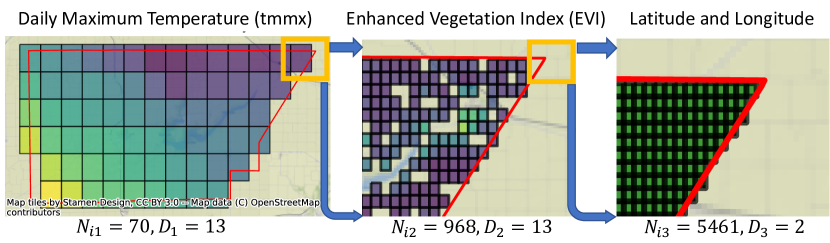
Figure 1: Visualisation of different resolutions within a county. The number of pixels $N_{il}$ vary between resolutions $l$.

Taking the enhanced vegetation index (EVI) from the MODIS (Didan, 2015) satellite system, observed over a county, as an example, the EVI is observed every 13 days at 250m spatial resolution, and as illustrated in Figure 1, each county will contain a distinct number of pixels spatially. It is therefore natural to model county level responses based on the similarity between the sets of pixels in different counties. Although the covariates are available as sets, we would like to see them as finite samples from a distribution. Intuitively, if we could measure at infinitely high resolution, then under the infinite limit, the empirical distribution of the set would converge to a distribution. An alternative approach would be to directly model the sets, as proposed in Deep Sets (Zaheer et al., 2017), but these have not shown to be competitive compared to kernel methods Lemercier et al. (2021b), which we will use.

We assume that the data comes in the form of $\{(\Pi_{i},y_{i})\}_{i=1}^{n}$, where $y_{i}\in\mathbb{R}$ is a label, $\Pi_{i}$ is a distribution over covariates $x\in\mathcal{X}$, where $\mathcal{X}$ is a Banach space e.g. $\mathcal{X}\subseteq\mathbb{R}^{d}$ for $d\in\mathbb{N}_{+}$ (Law et al., 2018a) or $d$-dimensional time series (Lemercier et al., 2021b). As in Lemercier et al. (2021b), define $\mathcal{P}(\mathcal{X})$ to be the space of distributions on $\mathcal{X}$. We focus on probability measures $\mathcal{P}(\mathcal{X})$ but note that arguments with finite measures are almost identical.

We denote $\mathcal{N}(a,b)$ as the distribution and $N(\cdot;a,b)$ the density function of a Gaussian distribution with mean $a$ and covariance $b$. In practice, $\Pi_{i}$ is not known explicitly and is estimated with the empirical measure $\hat{\Pi}_{i}=N_{i}^{-1}\sum_{j=1}^{N_{i}}\delta_{x_{ij}}$ for a bag of pixels $\{x_{ij}\}_{j=1}^{N_{i}}$, where $\delta_{x_{ij}}$ is a Dirac measure centred at $\{x_{ij}\}$ and $N_{i}\in\mathbb{N}_{+}$. Alternatively, one also could use survey weights (Law et al., 2018a) or model the weights using stochastic processes (Hamelijnck et al., 2019).

Gaussian processes (Rasmussen, 2003) have proven to be a versatile family of probabilistic models for a variety of problems in spatial statistics (Gelfand, 2010). We can define a Gaussian process over distributions as $f\sim\mathcal{GP}(0,\rho)$ with a kernel $\rho:\mathcal{P}(\mathcal{X})\times\mathcal{P}(\mathcal{X})\rightarrow\mathbb{R}$ that is positive definite. Just as regular Gaussian processes, for any $\Pi_{1},\ldots,\Pi_{n}\in\mathcal{P}(\mathcal{X})$ with $n\in\mathbb{N}_{+}$, $(f(\Pi_{1}),\ldots,f(\Pi_{n}))^{\intercal}\sim\mathcal{N}(0,K)$, where $K_{ij}=\rho(\Pi_{i},\Pi_{j})$. To choose a suitable kernel, we can first define a kernel $k$ over $\mathcal{X}$ such that $k:\mathcal{X}\times\mathcal{X}\rightarrow\mathbb{R}$ and define the kernel mean embeddings (Muandet et al., 2016)

$$\textstyle\mu_{P}(\cdot):=\int_{\mathcal{X}}k(\cdot,x)\text{d}P(x)\in\mathcal{H}_{k},$$

where $\mathcal{H}_{k}$ is the reproducing kernel Hilbert space (RKHS). With $\mathcal{H}_{k}$, we can now measure the similarity between distributions by the similarity between kernel mean embeddings via the inner product and norm of $\mathcal{H}_{k}$:

$$\textstyle\langle\mu_{P},\mu_{Q}\rangle_{\mathcal{H}_{k}}= \textstyle\int_{\mathcal{X}}\int_{\mathcal{X}}k(x,x^{\prime})\text{d}P(x)\text{d}Q(x^{\prime}),$$ (1)

$$\textstyle||\mu_{P}-\mu_{Q}||_{\mathcal{H}_{k}}^{2}= \textstyle\langle\mu_{P},\mu_{P}\rangle_{\mathcal{H}_{k}}+\langle\mu_{Q},\mu_{Q}\rangle_{\mathcal{H}_{k}}-2\langle\mu_{P},\mu_{Q}\rangle_{\mathcal{H}_{k}},$$

obtained using the kernel trick. This allows us to define a linear kernel $\rho(P,Q)=\langle\mu_{P},\mu_{Q}\rangle_{\mathcal{H}_{k}}$ or a squared exponential kernel $\rho(P,Q)=\sigma^{2}\exp\left(-||\mu_{P}-\mu_{Q}||_{\mathcal{H}_{k}}^{2}/(2\ell^{2})\right)$, where $\sigma,\ell>0$. Lastly, given empirical measures $\hat{P},\hat{Q}$, we can estimate Equation 1 with Monte Carlo integration

$$\textstyle\langle\mu_{P},\mu_{Q}\rangle_{\mathcal{H}_{k}}\approx\langle\mu_{\hat{P}},\mu_{\hat{Q}}\rangle_{\mathcal{H}_{k}}=\frac{1}{N_{i}N_{j}}\sum_{l,m}k(x_{il},x_{jm}),$$

where $x_{il}\stackrel{{\scriptstyle iid}}{{\sim}}P$ and $x_{jm}\stackrel{{\scriptstyle iid}}{{\sim}}Q$.

Aggregated Gaussian Processes:

A closely connected relative of Gaussian Processes over distributions are aggregated Gaussian processes (Law et al., 2018a; Hamelijnck et al., 2019; Tanaka et al., 2019; Yousefi et al., 2019; Lucas et al., 2020; Arambepola et al., 2020), where

$$\textstyle y_{i}=\int_{\mathcal{X}}f(x)\text{d}\Pi_{i}(x)+\epsilon_{i},\qquad\epsilon_{i}\sim\mathcal{N}(0,\sigma^{2}),$$ (2)

where $f\sim\mathcal{GP}(m,k)$, $\Pi_{i}\in\mathcal{P}(\mathcal{X})$ and $\epsilon_{i}$ is an independently distributed Gaussian noise with $\sigma>0$. $m$ and $k$ are the mean and covariance functions (for time series $\mathcal{X}$, $k$ could be the signature kernel (Toth and Oberhauser, 2020; Lemercier et al., 2021a)). The aggregated Gaussian processes construction has a very intuitive interpretation: the crop yield (measured in bushels per acre) for county $i$ is the average of the yields at the pixels containing croplands throughout the county. Using $\hat{\Pi}_{i}$, Equation 2 becomes

$$\textstyle y_{i}=\mathbf{w}_{i}^{\intercal}\mathbf{f}_{i}+\epsilon_{i},\qquad\epsilon_{i}\sim\mathcal{N}(0,\sigma^{2}),$$ (3)

where $\mathbf{f}_{i}\vcentcolon=(f(x_{i1}),\ldots,f(x_{iN_{i}}))^{\intercal}$, and $\mathbf{w}_{i}\vcentcolon=(w_{i1},\ldots,w_{iN_{i}})^{\intercal}$. Similarly, denote $\mathbf{f}_{*}\vcentcolon=(f_{*1},\ldots,f_{*N_{*}})^{\intercal}$ for prediction points $\{x_{*j},w_{*j}\}_{j=1}^{N_{*}}$ with true label $y_{*}$. Suppose further that $\mathbf{X}_{i}\vcentcolon=(x_{i1},\ldots,x_{iN_{i}})^{\intercal}$, $\mathbf{X}_{*}\vcentcolon=(x_{*1},\ldots,x_{*N_{*}})^{\intercal}$ and $k_{\mathbf{X}_{i}\mathbf{X}_{j}}:=(k(x_{il},x_{jm}))_{l,m}$ for pairs $i,j$, and $l=1,\ldots,N_{i}$ and $m=1,\ldots,N_{j}$,

With $(K)_{ij}=(\mathbf{w}_{i}^{\intercal}k_{\mathbf{X}_{i}\mathbf{X}_{j}}\mathbf{w}_{j})_{ij}$, $(K_{*})_{i}:=(\mathbf{w}_{i}^{\intercal}k_{\mathbf{X}_{i}\mathbf{X}_{*}}\mathbf{w}_{*})_{i}$ and $K_{**}:=\mathbf{w}_{*}^{\intercal}k_{\mathbf{X}_{*}\mathbf{X}_{*}}\mathbf{w}_{*}$, the posterior is $\mathbf{w}_{*}^{\intercal}\mathbf{f}_{*}|y\sim\mathcal{N}(\tilde{m}_{\mathbf{X}_{*}},\tilde{k}_{\mathbf{X}_{*}\mathbf{X}_{*}})$ with

$$\textstyle\tilde{m}_{\mathbf{X}_{*}} \textstyle\vcentcolon=\mathbf{w}_{*}^{\intercal}m_{\mathbf{X}_{*}}+K_{*}^{\intercal}(K+\sigma^{2}I_{n})^{-1}(y-m_{\mathbf{X}}),$$

$$\textstyle\tilde{k}_{\mathbf{X}_{*}\mathbf{X}_{*}} \textstyle\vcentcolon=K_{**}-K_{*}^{\intercal}(K+\sigma^{2}I_{n})^{-1}K_{*}.$$

If elements of $\mathcal{P}(\mathcal{X})$ are known explicitly, we can replace the entries of $K,K_{*}$ and $K_{**}$ with exact integrals e.g. $K_{ij}=\int_{\mathcal{X}}\int_{\mathcal{X}}k(x,x^{\prime})\text{d}P(u)\text{d}Q(v)$. Having inferred the posterior distribution of $f$ itself, it is then possible to directly query $f$ at the pixel level (Law et al., 2018a), or disaggregate, which can been used, e.g. for providing policy guidance in Malaria prevalence mapping (Lucas et al., 2020; Arambepola et al., 2020). In addition, one can also query an unseen bag-level aggregate $\mathbf{w}_{*}^{\intercal}\mathbf{f}_{*}$.

Connection to Gaussian Processes over Distributions:

We now establish the equivalence between aggregated Gaussian process and Gaussian processes over distributions with the kernel $\rho(P,Q)=\langle\mu_{P},\mu_{Q}\rangle_{\mathcal{H}_{k}}$. If we consider a Gaussian process $g\sim\mathcal{GP}(0,\rho)$ with a distributional kernel $\rho$, then it can be shown that (2) with $f\sim\mathcal{GP}(0,k)$, for any $\Pi_{1},\ldots,\Pi_{n}\in\mathcal{P}(\mathcal{X})$,

$$\textstyle(\int f\text{d}\Pi_{1},\ldots,\int f\text{d}\Pi_{n})^{\intercal},\quad\text{and}\quad(g(\Pi_{1}),\ldots,g(\Pi_{n}))^{\intercal}$$

are equal in distribution, since $\rho(P,Q)=\int\int k(x,x^{\prime})\text{d}P(x)\text{d}Q(x^{\prime})$ for any $P,Q\in\mathcal{P}(\mathcal{X})$. However, this equivalence breaks down if we consider a potentially nonlinear $\rho$. In addition, despite the 2 models being equivalent, we cannot simply establish that $g(P)=\langle f,\mu_{P}\rangle_{\mathcal{H}_{k}}=\int f\text{d}P$ since $f$ lies outside of $\mathcal{H}_{k}$ almost surely (Kanagawa et al., 2018). A major disadvantage of both Gaussian processes is the need to perform $\mathcal{O}(\sum_{i,j=1}^{n}N_{i}N_{j})$ number operations to compute the matrix $K$, and a subsequent $\mathcal{O}(n^{3})$ to invert $K+\sigma^{2}I_{n}$, therefore prohibiting the ability to efficiently tune the hyperparameters via maximum likelihood or sample via Markov chain Monte Carlo.

Variational Aggregated Gaussian Processes:

A major advantage for aggregated Gaussian processes, compared to Gaussian processes over distributions, is that the using a sparse variational Gaussian process approximation (SVGP; Hensman et al. (2013, 2015)) on aggregated Gaussian processes allows us to overcome the main computational bottleneck of distribution regression methods. VBAgg (Law et al., 2018a; Yousefi et al., 2019) proposes that we approximate $f$ directly with SVGP, making the approximation more feasible and allowing us to learn model hyperparameters via optimisation methods in mini-batches (Salimbeni et al., 2018; Adam et al., 2021) in $\mathcal{O}(M^{3}+M^{2}\sum_{i=1}^{n_{b}}N_{i})$ for a batch size of $n_{b}$ and $M$ inducing points. Although we could also use the viewpoint from $g$ to formulate a sparse variational approximation of $g$, it is not clear how to select and learn the inducing points, which lie in $\mathcal{P}(\mathcal{X})$. Even if we were able to do so, we would also need multiple inducing distributions, potentially still making the variational approximation very expensive. In addition, it is even more difficult as we only have access to empirical versions of elements in $\mathcal{P}(\mathcal{X})$.

Data Preprocessing for Earth Observation Data:

Figure 1 illustrates the spatial resolutions of the different covariates of interest at De Witt County, Illinois, United States. We can see that each resolution contains pixels of varying sizes and different numbers of observations at different spatial locations, which was previously not addressed in past works for aggregated Gaussian processes. Note: each resolution $l$ may also contain multiple different covariates (with dimension equalling $D_{l}$). To compute the distributional kernel in Equation 1, we have to sample from $\Pi_{i}$, which is the joint distribution over all covariates and resolutions, requiring resolution matching to sample from it.

Solutions that practitioners typically use (see Figure 2) are (1) Data-Agg: aggregating the covariates to a single resolution, typically the lowest resolution; (2) Data-Rep: repeat the pixels for the lower resolutions and obtain a potentially very large bag, if pixels at all resolutions are nested at each spatial location. To do this, we note that a pixel in the highest resolution lies in a nested set of lower resolution pixels from the other covariates, with each pixel having a single value associated with it. Data-Agg is commonly used and may result in loss of distributional information due to the aggregation, which we demonstrate in our experiments. Data-Rep may create large bags that are computationally infeasible, or if we subsample the data there may again be excessive losses of distributional information.

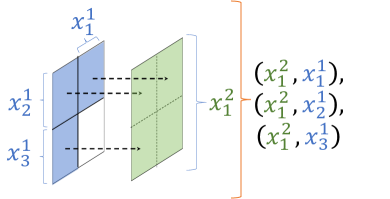
(a) Data-Rep

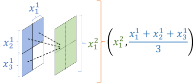
(b) Data-Agg

Figure 2: Data preprocessing methods for Earth observation data.

3 Multiresolution Aggregated Gaussian Processes

We propose Multiresolution Aggregated Gaussian Processes (MAgg) by exploiting the structure of additive kernels (Duvenaud et al., 2011) within aggregated Gaussian processes. We show that our model better handles the multiresolution nature of Earth observation data by minimising the amount of data preprocessing needed, whilst retaining the computational advantages of sparse variational aggregated Gaussian processes and gaining additional interpretability.

Let $\mathcal{X}=\mathcal{X}^{1}\times\cdots\times\mathcal{X}^{d}$ and $\Pi$ have marginal distributions $\Pi^{1}\ldots\Pi^{d}$. The constant $d$ denotes the number of different resolutions, in which each itself may also contain different covariates. Treating each bag of covariates as a distribution, for each response $y_{i}$ we have the marginal distributions $\Pi^{1}_{i}\in\mathcal{P}(\mathcal{X}^{1}),\ldots,\Pi^{d}_{i}\in\mathcal{P}(\mathcal{X}^{d})$. We integrate an additive Gaussian process $f$

$$\textstyle y_{i} \textstyle=\int_{\mathcal{X}}f(x)\text{d}\Pi_{i}(x)+\epsilon_{i}$$

$$\textstyle=\sum_{l=1}^{d}\int_{\mathcal{X}^{l}}f^{l}(x^{l})\text{d}\Pi_{i}^{l}(x^{l})+\epsilon_{i},\epsilon_{i}\sim\mathcal{N}(0,\sigma^{2}),$$

where $f\sim\mathcal{GP}(0,\sum_{l}k_{l})$ and $f^{l}\sim\mathcal{GP}(0,k_{l})$ with $k^{l}:\mathcal{X}^{l}\times\mathcal{X}^{l}\rightarrow\mathbb{R}$. Each Gaussian process $f^{l}$ only depends on the $l$th resolution, meaning that we only need to consider integrating over the marginal distribution $\Pi^{l}$, enabling us to circumvent any resolution matching.

We may also model the interaction between different covariates at different resolutions using the additive kernel of Duvenaud et al. (2011) and thus the corresponding aggregated model

$$\textstyle y_{i}= \textstyle\int f^{1}\text{d}\Pi_{i}^{1}+\cdots+\int f^{12}\text{d}\Pi_{i}^{12}+\cdots+\int f^{1\cdots d}\text{d}\Pi_{i}^{1\cdots d}+\epsilon_{i},\qquad\epsilon_{i}\sim\mathcal{N}(0,\sigma^{2}),$$

where $f\sim\mathcal{GP}(0,\sigma_{1}^{2}\sum_{l=1}^{d}k^{l}+\sigma_{2}^{2}\sum_{l,m:l\neq m}k^{l}k^{m}+\cdots+\sigma_{d}^{2}\prod_{l=1}^{d}k^{l})$, $\sigma_{1}\ldots,\sigma_{d}>0$ are scale factors for each order of interaction and $\Pi^{u}_{i}$ is the joint distribution over a set of resolutions $u$ for $u\subseteq[d]=\{1,\ldots,d\}$.

Denote the inner product distributional kernel in Equation 1 as $\bar{\Pi}^{u}_{i}\Pi^{u}_{j}[k^{u}]:=\int\int\prod_{l\in u}k^{l}(x,x^{\prime})\text{d}\Pi^{u}_{i}(x)\text{d}\Pi^{u}_{j}(x^{\prime})$, where $u\subseteq[d]$. To compute the variance of $\int f\text{d}\Pi_{i}$, which reduces to computing $\bar{\Pi}_{i}\Pi_{j}[k]$, one can decompose the integral into

$$\textstyle\bar{\Pi}_{i}\Pi_{j}[k] \textstyle=\sigma_{1}^{2}\sum_{l=1}^{d}\bar{\Pi}_{i}^{l}\Pi_{j}^{l}[k^{l}]+\cdots+\sigma_{d}^{2}\bar{\Pi}_{i}^{1\cdots d}\Pi^{1\cdots d}_{j}[\prod_{l=1}^{d}k^{l}],$$

where we can compute each term in the total summation with the empirical distribution $\hat{\Pi}^{u}_{i}$ for the subset of resolutions $u$. The advantage of this decomposition is that for each $\hat{\Pi}^{u}_{i}$, resolution-matching (see Section 2) only needs to occur between resolutions in $u$. For $\Pi_{i}^{1\cdots d}$, the joint distribution over all resolutions, we match all resolutions as for VBAgg. However, to compute the first order effects we do not require any preprocessing at all, leaving us with the original $N_{il}$ number of pixels. For second order effects, given resolutions $l$ and $h$, we only need to resolution-match the $N_{il}$ and $N_{ih}$ number of pixels from each resolution.

Variational Inference:

We propose MVBAgg, a SVGP approximation to our model. Although we have constructed an additive kernel that aggregates each component separately, we still need to address the computational bottleneck of aggregated Gaussian processes with SVGP (Hensman et al., 2013, 2015). Since the sample path is $f=f^{1}+\cdots+f^{1\ldots d}:\mathcal{X}\rightarrow\mathbb{R}$, this suggest that we can still define the usual inducing variables by selecting $M$ inducing points $\mathbf{Z}=(z_{1},\ldots,z_{M})^{\intercal}\subset\mathcal{X}$, and setting the inducing variable to be $\mathbf{u}=f(\mathbf{Z})\equiv(f(z_{1}),\ldots,f(z_{M}))^{\intercal}$. Similar to Law et al. (2018a), we select $\mathbf{Z}$ by first applying Data-Rep to each training bag and then picking 1 cluster centre selected via KMeans. This step is only done outside the training loop to initialise the inducing points, so that we can take into account of correlations between resolutions and preserve distributional information, and is feasible as KMeans is very scalable. One may also pick a cluster centre for each resolution and then concatenate to obtain the subsequent inducing point for a bag, yielding similar $\mathbf{Z}$’s but losing some inter-resolution correlations.

We pose a variational distribution $q(f,\mathbf{u})\vcentcolon=p(f|\mathbf{u})q(\mathbf{u})$ and construct a variational approximation $q(\mathbf{u})=\text{argmin}_{q\in\mathcal{Q}}\text{KL}(q(f,\mathbf{u})||p(f,\mathbf{u}|y))$. We choose the variational family $\mathcal{Q}=\{q(\mathbf{u})=N(\mathbf{u};\mathbf{m},\mathbf{S}):\mathbf{m}\in\mathbb{R}^{M},\mathbf{S}\in\mathbb{R}^{M\times M}\}$. We thus have the approximate posterior $q(f)\vcentcolon=\int p(f|\mathbf{u})q(\mathbf{u})\text{d}\mathbf{u}\equiv\mathcal{GP}(f;\tilde{m},\tilde{k})$ where

$$\textstyle\tilde{m}(x)=k_{x\mathbf{Z}}\alpha,\quad\tilde{k}(x,x^{\prime})=k_{xx^{\prime}}-k_{x\mathbf{Z}}\mathbf{Q}^{-1}k_{\mathbf{Z}x^{\prime}},$$

where $\alpha=k_{\mathbf{Z}\mathbf{Z}}^{-1}\mathbf{m}$ and $\mathbf{Q}^{-1}=(k_{\mathbf{Z}\mathbf{Z}}^{-1}-k_{\mathbf{Z}\mathbf{Z}}^{-1}\mathbf{S}k_{\mathbf{Z}\mathbf{Z}}^{-1})$. Aggregating gives $\int f\text{d}\Pi_{i}\sim\mathcal{N}\bigg{(}\Pi_{i}[\tilde{m}],\bar{\Pi}_{i}\Pi_{i}[\tilde{k}]\bigg{)}$, where $\Pi_{i}[\tilde{m}]=\int\tilde{m}(x)\text{d}\Pi_{i}(x)$. Denoting

$$\textstyle\Pi_{i}^{u}[k^{u}_{\cdot\mathbf{Z}}] \textstyle:=\int\prod_{l\in u}k^{l}_{x\mathbf{Z}}\text{d}\Pi^{u}_{i}(x),\quad\Pi_{i}^{u}[k^{u}_{\mathbf{Z}\cdot}]:=\Pi_{i}^{u}[k^{u}_{\cdot\mathbf{Z}}]^{\intercal},$$

where $u\subseteq[d]$, we have

$$\textstyle\Pi_{i}[k_{\cdot\mathbf{Z}}] \textstyle=\sigma_{1}^{2}\sum_{l=1}^{d}\Pi_{i}^{l}[k^{l}_{\cdot\mathbf{Z}}]+\cdots+\sigma_{d}^{2}\Pi^{1\cdots d}_{i}[\prod_{l=1}^{d}k^{l}_{\cdot\mathbf{Z}}],$$

$$\textstyle\bar{\Pi}_{i}\Pi_{i}[k] \textstyle=\sigma_{1}^{2}\sum_{l=1}^{d}\bar{\Pi}^{l}_{i}\Pi^{l}_{i}[k^{l}]+\cdots+\sigma_{d}^{2}\bar{\Pi}_{i}^{1\cdots d}\Pi_{i}^{1\cdots d}[\prod_{l=1}^{d}k^{l}],$$

giving

$$\textstyle\Pi_{i}[\tilde{m}] \textstyle=\Pi_{i}[k_{\cdot\mathbf{Z}}]\alpha,$$

$$\textstyle\bar{\Pi}_{i}\Pi_{i}[\tilde{k}] \textstyle=\bar{\Pi}_{i}\Pi_{i}[k]-\Pi_{i}[k_{\cdot\mathbf{Z}}]\mathbf{Q}^{-1}\Pi_{i}[k_{\mathbf{Z}\cdot}].$$

We see that each pair of $\Pi^{u}_{i}[k^{u}_{\cdot\mathbf{Z}}]$ and $\bar{\Pi}^{u}_{i}\Pi^{u}_{i}[k^{u}]$ can be aggregated with respect to its own resolution using $\Pi_{i}^{u}$ again. With the empirical measures $\hat{\Pi}^{u}_{i}$, we have the approximations $\Pi^{u}_{i}[k^{u}_{\cdot\mathbf{Z}}]\approx(\mathbf{w}_{i}^{u})^{\intercal}k_{\mathbf{X}_{i}^{u}\mathbf{Z}}$ and $\bar{\Pi}_{i}^{u}\Pi^{u}_{i}[k^{u}]\approx(\mathbf{w}_{i}^{u})^{\intercal}k_{\mathbf{X}_{i}^{u}\mathbf{X}_{i}^{u}}\mathbf{w}_{i}^{u}$. Note that we cannot apply the Newton-Girard rule for computing additive kernels (Duvenaud et al., 2011) since the distributions $\Pi^{u}_{i}$ for $u\subseteq[d]$ are not a product distributions in general (i.e. independence between resolutions). However, for practical applications such as crop yield modelling, it may be sufficient to use only 3-4 data sources (each with a different resolution) and limit the order of interactions to 2, giving us $d+d(d-1)/2$ terms to compute. Indeed as discussed in Duvenaud et al. (2011), many problems may not require very high orders of interactions.

Lastly, the hyperparameters, such as the kernel parameters, can be learned via maximisation of the lower bound

$$\textstyle\mathcal{L}\vcentcolon=\text{KL}(q(\mathbf{u})||p(\mathbf{u}))-\sum_{i=1}^{n}\mathbb{E}_{q(f)}[\log p(y_{i}|\int f\text{d}\Pi_{i})],$$

and solved via optimisation methods in mini-batches (Salimbeni et al., 2018; Adam et al., 2021) again. We note that non-Gaussian likelihoods $p(y_{i}|\int f\text{d}\Pi_{i})$ are also possible, such as Poisson (Law et al., 2018b) or Binomial. Inheriting the nice properties of VBAgg, with order 1 interactions for instance, we can attain $\mathcal{O}(M^{3}+M^{2}\sum_{l=1}^{d}\sum_{i=1}^{n_{b}}N_{il})$ complexity per iteration.

Interpretability:

We can disaggregate or make pixel-level predictions for each component $f^{1},\ldots,f^{12},\ldots,f^{1\cdots d}$, which are functions at the covariate resolution. Despite the non-identifiability of each function (our estimates of each function will always have a constant bias), we may nonetheless interpret the gradients of the disaggregated maps (Law et al., 2018a; Lucas et al., 2020; Agarwal et al., 2020) for decision-making. Post-training, the multiresolution viewpoint allows disaggregation of $f$ at the highest resolution if we use Data-Rep to obtain a single vector $x$ for all the covariates at the highest resolution, for which we can use to calculate the posterior distribution of $f(x)$. In comparison, VBAgg with Data-Agg only has 1 resolution to disaggregate to because all the resolutions have already been matched.

Another way to gain interpretability from aggregated Gaussian processes is to determine the covariate sensitivity. For simplicity, only considering 1st order interactions, we can calculate the 1st and 2nd order Sobol indices (Sobol’, 1990):

$$\textstyle S_{l}=\frac{\text{Var}_{x}[{\tilde{m}^{l}(x_{l})}]}{\text{Var}_{x}[\tilde{m}(x)]+\sigma^{2}},S_{u}=\frac{2\text{Cov}_{x_{l},x_{h}}[\tilde{m}^{l}(x_{l}),\tilde{m}^{h}(x_{h})]}{\text{Var}_{x}[\tilde{m}(x)]+\sigma^{2}},$$

where $u=\{l,h\}$ is a tuple and we approximated each Sobol index term with Monte Carlo using the entire dataset obtained with Data-Rep for MVBAgg. The 1st order Sobol indices indicate how much the variance is explained by each resolution on its own, and the 2nd order Sobol indices between pairs of resolutions. We note that $\sum_{l=1}^{d}S_{l}+\sum_{u:u=(l,h)}S_{u}+\sigma^{2}=1$ and it also possible to consider higher order Sobol indices to take into account of more interactions. Additionally, we can also compute the Sobol indices for each distribution $\Pi_{i}$ to obtain local sensitivity analysis within each bag, for which the Var and Cov operators are integrated with respect to $\Pi_{i}$. More details on the approximate of Sobol indices is in Appendix B.

4 Related Work

Aggregated Gaussian Processes:

In previous aggregated Gaussian process works, all the resolutions are usually preprocessed to the same resolution (Law et al., 2018a; Tanaka et al., 2019; Yousefi et al., 2019; Hamelijnck et al., 2019; Arambepola et al., 2020; Lucas et al., 2020). As mentioned at the start of Section 3, this may have disadvantages. In contrast, our model only requires full resolution matching if we use the highest order of interaction within the additive kernel. In the context of classification of images, alternative aggregation methods are max-aggregation or attention-aggregation (Kim and De la Torre, 2010; Haussmann et al., 2017; Ilse et al., 2018), which are special cases of $\Pi_{i}=\delta(\max_{x\in N_{i}^{\complement}})$, where $N_{i}=\bigcup_{N\in\mathcal{F}}N$ such that $\Pi_{i}(N)=0$, the union of all sets in $\mathcal{X}$ with zero measure under $\Pi_{i}$. In the spatial statistics literature (Gelfand, 2010; Diggle et al., 2013; Wilson and Wakefield, 2020), what are referred to as spatially aggregated or Gaussian processes over areal data are also aggregated Gaussian processes.

Disaggregation:

Deconditional mean embeddings (Chau et al., 2021) and 2-staged ridge regression (Stefanovic et al., 2021) have recently used for disaggregation, although both methods require mediating variables at the same resolution as the response, which is less related to the challenges that we address in this paper. Additionally, Law et al. (2018b); Hamelijnck et al. (2019); Lucas et al. (2020); Arambepola et al. (2020) all address the problem of disaggregation for the purpose of public policy guidance but only for single, preprocessed resolutions obtain with Data-Agg, whereas our model is able to disaggregate at the highest resolution and better maintain fine-scale covariate information.

Multiresolution Regression:

Multiresolution Gaussian processes (Fox and Dunson, 2012; Taghia and Schön, 2019) and kernels (Cuturi and Fukumizu, 2005) assume that there is a nested partition of $\mathcal{X}$. This setting would be equivalent to applying Data-Agg to match all resolutions to one, if there exists a nested structure. In our case, we do not assume that there is always such a structure, which helps us increase the number of Monte Carlo points we can use for lower order interactions. Furthermore, Rudner et al. (2018) developed $\text{Multi}^{3}\text{net}$ to also handle the multi-resolution nature of different satellite imageries for regression. In their work, they used an ensemble of independent neural networks to learn from multiresolution images, whereas we consider more parameter efficient models through kernels and learn from set or distribution-valued inputs.

Our work is also closely related to multi-source distribution regression of Thorns (2018); Adsuara et al. (2019), where the aggregations are also done over separate resolutions. In their works, they consider distribution regression fitted via random Fourier features (Rahimi and Recht, 2008) and Bayesian distribution regression (Law et al., 2018b), which yield similar computational complexities as MVBAgg and are both applied to crop yield prediction. However, both works only consider bag-level predictions, whereas we also study disaggregation.

Distribution Regression:

Closely related to Gaussian processes over distributions, distribution regression (Szabó et al., 2016) also provides a family of frequentist regression methods to learn from distributions. A regression function $f\in\mathcal{H}_{\rho}$ is learned via regularised least squares over the dataset $\{(\mu_{\hat{\Pi}_{i}},y_{i})\}_{i=1}^{n}$. Distribution regression methods have been successfully applied to crop yield prediction (Thorns, 2018; Adsuara et al., 2019; Lemercier et al., 2021b), election forecasting (Flaxman et al., 2016) and sequential data (Lemercier et al., 2021b). Bayesian approaches can also be used to model within-bag variations of the covariates for downstream regression tasks (Law et al., 2018b). To note, although not done explicitly for existing works, for both Gaussian processes over distributions and distribution regression, it is also possible to make ‘individual level’ predictions at the Dirac measures $\delta_{x_{ij}}$.

Crop Yield Modelling:

Our main experiment models crop yields using climatic and satellite data, which are also widely used in previous works (Burke et al., 2021). Many previous works have either spatially averaged the pixels for each county (Mateo-Sanchis et al., 2019; Sanchis et al., 2019; Martínez-Ferrer et al., 2020; Han et al., 2020; Fan et al., 2021) or summarised the spatially-distributed pixels into an empirical distribution (histogram) (You et al., 2017). You et al. (2017) assumes permutation invariance of the pixels, which we also assume, but our method would retain more distributional information as we implicitly use empirical kernel mean embeddings. Brus et al. (2018) also studies disaggregation for crop yields using aggregated Gaussian processes, but models all other covariates other than longitude and latitude using a linear model.

5 Experiments

We demonstrate the predictive performance of MVBAgg compared to VBAgg, Random Forest and a Gaussian process regression model (CGP) with centroid covariates. For VBAgg, we apply Data-Agg via mean aggregation to the lon-lat and MODIS covariates match them to GRIDMET resolution. As noted in Table 1, we apply Data-Agg to the lon-lat and MODIS covariates to slightly upsample them from 30m to 500m and 250 to 1000m resolutions respectively, due to the sheer size of the data. For simplicity, we ignore the temporal resolution in the experiments by concatenating the temporal resolution at each spatial location to work with a 13-dimensional vector. The time window taken is between April and October, which was noted in Mateo-Sanchis et al. (2019) as the crop growth window. Since the MODIS covariates are measured every 13 days, we take samples for GRIDMET covariates on the same days as well. Lastly, we do not apply a crop mask for lon-lat due to the fact that the distributions are uniform distributions (i.e. measures of area).

When training VBAgg and MVBAgg, we perform natural gradient descent (Salimbeni et al., 2018) to learn $q(\mathbf{u})$ and learn all other hyperparameters with the Adam optimiser. Details of each model and configurations are available in Appendix B. We use 1st order interactions for simplicity. For computational tractability during training, we restrict the maximum bag size to $N_{i}=100$ for MODIS and GRIDMET covariates, and $N_{i}=500$ for lon-lat, via random subsampling with each bag. This is because for MODIS, the bag sizes can range from 67 to 5950, whereas for lon-lat the range is between $2399$ to $34867$. We evaluate the predictive performance in estimating $y_{i}$ via the test loglikelihood (LL; higher is better) and root mean squared error (RMSE; lower is better). Our implementation (see Appendix C) relies on GPFlow (De G. Matthews et al., 2017), and all data and code will be made available upon publication.

Table 1: Collected datasets and their associated descriptions. We slightly downsampled the EVI from 250m to 1000m and latitude, longitude from 30m to 500m due to computational constraints in obtaining the dataset.

Data Source Resolution Soybean mask USDA NASS Cropmask (NASS, 2016) 30m latitude, longitude ($D_{1}=2$) USDA NASS Cropmask (NASS, 2016) 500m EVI ($D_{2}=13$) MODIS (Didan, 2015) 1000m pr, tmmx ($D_{3}=26$) GRIDMET (Abatzoglou, 2013) 4638.3m Soybean yield USDA National Agricultural Statistics Service. (NASS, 2017) US County

Table 2: Predictive performance over 5 different randomly selected set of counties. We report the average test LL and RMSE, alongside their standard errors.

Method LL RMSE Random Forest NA 3.236$\pm 0.5975$ CGP 0.5779$\pm 0.09628$ 0.9458$\pm 0.06792$ VBAgg 0.6976$\pm 0.1771$ 0.9371$\pm 0.02296$ MVBAgg $\mathbf{0.9841\pm 0.1046}$ $\mathbf{0.6899\pm 0.1185}$

5.1 Semi-synthetic

We generate synthetic aggregated labels using real covariates from satellite imagery and weather features over croplands collected from Google Earth Engine (Gorelick et al., 2017). We include the covariates: latitude, longitude, enhanced vegetation index (EVI) on 7th April 2015, precipitation (pr) and maximum temperature (tmmx) on 7th April 2015. For data generation, we use the full bag and generate

$$\textstyle y_{i}= \textstyle\sum_{l=1}^{4}\frac{1}{N_{il}}\sum_{j=1}^{N_{il}}f^{l}(x_{ij}^{l})+\epsilon_{i},\quad\epsilon_{i}\sim\mathcal{N}(0,0.5^{2}).$$

£We let $f^{0}(x)=0.5(x_{\text{lon}}^{2}+x_{\text{lat}}^{2})$, $f^{1}(x)=x_{\text{EVI}}^{2}$, $f^{2}(x)=1.5x_{\text{pr}}^{2}$ and $f^{3}(x)=2x_{\text{tmmx}}^{2}$.

We report statistically signficant predictive results for MVBAgg in Table 2. A priori, we would expect CGP and Random Forest to perform worse as it only contains information about the first moments of each covariate distribution. In addition, we would not expect VBAgg to perform as well as MVBAgg due to (1) the preprocessing of the covariates to the GRIDMET resolution causes the distributions for latitude, longitude and EVI to be different from the underlying true aggregation distributions and (2) fewer points are used for Monte Carlo estimation of $\Pi_{i}[k_{\cdot\mathbf{Z}}]$ and $\bar{\Pi}_{i}\Pi_{i}[k]$.

In addition, we can also disaggregate MVBAgg and VBAgg to obtain the underlying functions $f^{l}$, as shown in Figure 3. Theoretically, it is expected that there are constant biases for each estimated $f^{l}$ because if the constant biases for each function cancel each other out, then they are also valid estimates for $f$. We therefore manually apply shifts to illustrate that we have indeed fitted each $f^{l}$ up to a constant shift. Although only having biased estimates of $f^{l}$, we can still interpret the gradient $f^{l}$ to make policy decisions (e.g. increases in EVI are associated with increases with yield) and $\text{Var}_{x}[f^{l}(x)]$ (e.g. to compute feature sensitivity). We see that the disaggregations for VBAgg and MVBAgg are very similar. In addition, the histogram of the EVI from all the bags shows that there are more values lying in $[-1,0]$ in the original data compared to the aggregated data that VBAgg uses, and it coincides with the fact that the disaggregation within that interval is more accurate.

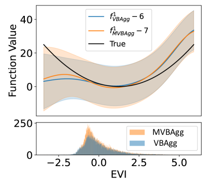
Figure 3: Disaggregation of $f^{1}$ (EVI covariates) via VBAgg and MVBAgg with 95% credible intervals. The histogram shows the EVIs values used for each model.

5.2 Crop Yield Modelling

By definition, crop yield is the average productivity/crop production per unit, which is in this case bushels/acre. Understanding crop yields can allow us to infer the fertility of the land as a function of climatic and satellite observations, allowing us to decide where to plant crops or which areas require policy interventions. We collected soybean yields (bushels/acre) from 2015 and 2017 for 384 counties in the crop belt of the United States (see Figure 4). We use the same covariates previously used for the semi-synthetic data and work with log-yields in order to remove any skew.

Figure 4: Soybean yields (bushels/acre) in the United States.

We randomly select sets of counties, train the models over 2015 data ($n=308$) and then make predictions for 2017 yields ($n=308$). In Table 3 and 4, we report the predictive performance and covariate sensitivities respectively. We see that MVBAgg again performs the best in terms of LL. The quality of bag-level predictions is in this case similar to CGP. We suggest that this is due to (1) the aggregation steps used for obtaining MODIS and lon-lat covariates due to computational constraints; (2) lack of additional informative covariates or (3) the crop yields only depend on the first moments of the covariates. Interestingly, we see that VBAgg performs a lot worse than CGP and MVBAgg, having aggregated both EVI and lon-lat covariates to GRIDMET’s resolution. Therefore there is evidence to suggest that the data preprocessing step to match resolutions of covariates actually has a detrimental effect on the model performance of VBAgg, even though VBAgg uses a more sophisticated aggregation model than CGP.

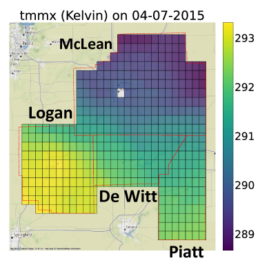
Figure 5: Disaggregation of $f^{3}$ (all 13 tmmx covariates) and observation of tmmx on the 7th of April, 2015. No disaggregations for Bloomington due to it being filtered out with the crop mask.

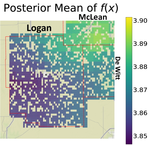
Figure 6: Disaggregation of $f$ (all covariates) and observation of tmmx on the 7th of April, 2015. No disaggregations at cities and rivers due to them being filtered out with the crop mask.

From Table 4, we also see that CGP explains the variance in the response differently to MVBAgg, but we note that CGP uses only the centroids as input and thus it only explains how the covariate means affect the response. In addition, the likelihood noise almost accounts for no variability, which may also not be a realistic assumption as in practice crop yields can have a lot of noise. On the other hand, VBAgg identifies a similar set of covariates, especially the EVI, and seems to attribute a lot of the variance due to spatial randomness (i.e. lonlat). The likelihood noise also accounts for a smaller percentage of variance compared to MVBAgg. Considering the poor predictive performance, this raises the suspicion that the resolution-matching has made VBAgg pick up incorrect signals from the aggregated EVI and overfitted on lon-lat. MVBAgg on the other hand lies between CGP and VBAgg, whilst being able to explain covariates at higher resolutions with Data-Rep (VBAgg is limited to the covariates obtained via Data-Agg).

From Figure 5 and 6, we can see that the model assigns lower yields in Logan county, and the Sobol indices in Table 4 suggest that a large proportion of this can be explained by tmmx. Plotting 1 day out of 13 days of tmmx in 2015, we can see that Logan county saw relatively high temperatures, going up to 293. Soybean crops may fail at excessively high temperatures and it is probable that Logan county had consistently higher temperatures throughout the year than the other counties that made soybean yields lower.

Table 3: Predictive performance over 5 different randomly selected set of counties. We report the average test LL and RMSE, alongside their standard errors.

Method LL RMSE Random Forest NA 0.1071$\pm 0.002171$ CGP -0.7633$\pm 0.01650$ 0.1027$\pm 0.002082$ VBAgg -0.8482$\pm 0.01059$ 0.1139$\pm 0.001149$ MVBAgg $\mathbf{-0.7387\pm 0.01575}$ $\mathbf{0.1023\pm 0.002372}$

Table 4: Top 3 Sobol indices and estimated normalised likelihood variances based on 2015 data.

CGP VBAgg MVBAgg EVI (0.551) lonlat-EVI (0.251) tmmx (0.442) EVI-tmmx (0.332) EVI (0.231) lonlat-tmmx (0.186) lonlat-EVI (0.0222) lonlat (0.199) pr-tmmx (0.0647) $\frac{\sigma^{2}}{\text{Var}_{x}[\tilde{m}(x)]+\sigma^{2}}$  $7.06e-5$ 0.0894 0.185

6 Conclusion and Discussion

Motivated by the problem of crop yield modelling, where a crop yield response is paired with samples of many covariates collected from data sources of varying spatial resolutions, we propose a Gaussian process model to efficiently handle such multiple resolutions through an additive kernel structure and variational inference. Compared to existing approaches, we show that our method minimises the amount of data preprocessing needed to match between resolutions and better maintains all available distributional information. Through synthetic and real world crop yield modelling experiments, we demonstrate that commonly used data preprocessing techniques of matching resolutions via data aggregation can have negative consequences on the predictive performance and interpretability of aggregated Gaussian processes, and that our method overcomes these issues. We hope that the methodology and workflow developed in this work can be used for further scientific investigations into problems of similar settings, such as crop yield modelling, epidemiology and climate science.

Limitations and Future Directions:

In the alternative formulation with Gaussian processes defined over distributions, the aggregated Gaussian processes is restricted to the inner product second-level kernel, making the induced function space theoretically less expressive than general distributional kernels. Other types of kernels, however, do not admit an aggregated formulation, are less interpretable and it is unclear how to apply useful variational approximations to them. It would also be interesting to explore more expressive formulations of aggregated Gaussian processes, e.g. alternative aggregation operators.

In our experiments, for computational scalability, we subsampled each bag and set a limit on the number of items in each bag. However, given more computational resources, this may not be necessary and may yield better performances. We stress that the crop yield experiments presented here are only for demonstration purposes: we provide the modelling tools and workflow that may be able to generate impactful insights when combined with domain expertise, especially when deciding which type of satellite data and which covariates to use.

Appendix A Derivation of Aggregated Gaussian Process Posterior

Since we have

$$\textstyle\begin{pmatrix}y_{1}\\ \vdots\\ y_{n}\\ \mathbf{w}_{*}^{\intercal}\mathbf{f}_{*}\end{pmatrix}=\mathcal{N}\Bigg{(}\begin{pmatrix}\mathbf{w}_{1}^{\intercal}m_{\mathbf{X}_{1}}\\ \vdots\\ \mathbf{w}_{n}^{\intercal}m_{\mathbf{X}_{n}}\\ \mathbf{w}_{*}^{\intercal}m_{\mathbf{X}_{*}}\end{pmatrix},\begin{pmatrix}K+\sigma^{2}I_{n}&K_{*}\\ K_{*}^{\intercal}&K_{**}\end{pmatrix}\Bigg{)},$$

where $(K)_{ij}=(\mathbf{w}_{i}^{\intercal}k_{\mathbf{X}_{i}\mathbf{X}_{j}}\mathbf{w}_{j})_{ij}$, $(K_{*})_{i}:=(\mathbf{w}_{i}^{\intercal}k_{\mathbf{X}_{i}\mathbf{X}_{*}}\mathbf{w}_{*})_{i}$ and $K_{**}:=\mathbf{w}_{*}^{\intercal}k_{\mathbf{X}_{*}\mathbf{X}_{*}}\mathbf{w}_{*}$. We can thus obtain the posterior $\mathbf{w}_{*}^{\intercal}\mathbf{f}_{*}|y\sim\mathcal{N}(\tilde{m}_{\mathbf{X}_{*}},\tilde{k}_{\mathbf{X}_{*}\mathbf{X}_{*}})$ via standard multivariate Gaussian conditioning to get

$$\textstyle\tilde{m}_{\mathbf{X}_{*}} \textstyle\vcentcolon=\mathbf{w}_{*}^{\intercal}m_{\mathbf{X}_{*}}+K_{*}^{\intercal}(K+\sigma^{2}I_{n})^{-1}(y-m_{\mathbf{X}}),$$

$$\textstyle\tilde{k}_{\mathbf{X}_{*}\mathbf{X}_{*}} \textstyle\vcentcolon=K_{**}-K_{*}^{\intercal}(K+\sigma^{2}I_{n})^{-1}K_{*}.$$

If elements of $\mathcal{P}(\mathcal{X})$ are explicitly known, then we would obtain

$$\textstyle(K)_{ij} \textstyle\vcentcolon=\int_{\mathcal{X}}\int_{\mathcal{X}}k(u,v)\text{d}\Pi_{i}(u)\text{d}\Pi_{j}(v),$$

$$\textstyle(K_{*})_{i} \textstyle\vcentcolon=\int_{\mathcal{X}}\int_{\mathcal{X}}k(u,v)\text{d}\Pi_{*}(u)\text{d}\Pi_{i}(v),$$

$$\textstyle K_{**} \textstyle\vcentcolon=\int_{\mathcal{X}}\int_{\mathcal{X}}k(u,v)\text{d}\Pi_{*}(u)\text{d}\Pi_{*}(v).$$

Appendix B Experiments: Additional Information

In this section, we provide the details for how the data is obtained and processed. We also provide additional details for each experiment.

Data Engineering:

We obtained the covariates via the Google Earth Engine (GEE) Python API [Gorelick et al., 2017]. A Javascript-based code editor is available on the Google Earth Engine (GEE) website and allows for rapid visualisation of all the datasets within GEE. All the datasets we used are available on GEE. The key classes in GEE are Image, ImageCollection and MultiPolygon. Image stores information on a raster, or image, and ImageCollection stores a set of Image objects. MultiPolygon stores information on the geometries, or boundaries, of regions. For example, each county in our paper will have a corresponding boundary. With MultiPolygon, we can use the getRegion() method of ImageCollection to extract data, and hence pixels containing covariate data, only within the MultiPolygon geometry. We used geometries for US counties that are publicly available online, such as from https://public.opendatasoft.com/explore/dataset/us-county-boundaries/table/?disjunctive.statefp&disjunctive.countyfp&disjunctive.name&disjunctive.namelsad&disjunctive.stusab&disjunctive.state_name.

GEE objects are processed on the server-side via client-side requests. However, once processed on the server side, we can directly request the data to be transferred to the client-side if the data size is moderate calling the getInfo() method from any GEE object. Another option is to download the data to Google Drive or Cloud. Further information can be found here https://developers.google.com/earth-engine/tutorials/community/intro-to-python-api-guiattard.

• Masking: We applied a 30m resolution soybean mask [NASS, 2016] to both the MODIS and GRIDMET datasets. Since the soybean mask is at a much lower resolution than either datasets, we "max-downsampled" the mask to each resolution by defining a value as 0 if there are no cropland pixels in the lower resolution pixel, and 1 otherwise. This can be done in GEE via the Image methods reduceResolution() and updateMask(). Once the masking is done, we can collect the data using getRegion() on each MultiPolygon, which returns a long list of datetime, longitude, latitude and covariate values, for which we can store in a pandas.DataFrame object in Python. To obtain the longitude and latitude coordinates at 500m resolution, we used a similar procedure except that the covariates are also from the soybean mask ImageCollection.

• Aggregation: We note that we downsampled MODIS to 1000m resolution for MVBAgg and 4638.3m for VBAgg, after applying the mask. As just mentioned, we also downsampled the crop mask to 500m resolution to obtain longitude and latitude coordinates. Similar to max-downsampling, we can also use mean-downsampling using reduceResolution(). To do this, we use the mean reducer ee.Reducer.mean() as the argument inside reduceResolution(), instead of ee.Reducer.max(). This step essentially performs Data-Agg, as we discussed in the main section.

• Data-Rep: To match the pixels via repetition, suppose we have 2 DataFrame objects in Python, each representing a different resolution and have columns longitude, latitude and covariate values. We first take the lower resolution DataFrame, which we call df1, and use the Point object in the Shapely to create a Point for each row, using the longitude and latitude. A Point simply stores the longitude and latitude of the centre of the pixel but allows us to perform spatial operations in conjunction with the geopandas library. We then convert df1 into a GeoDataFrame in geopandas. Next, given that you know the spatial resolution of df2 (e.g. for 500m resolution, the spatial resolution would be 0.0089835 degrees), we create a square Polygon object for each row, representing the boundaries of each pixel, and then also convert it to a GeoDataFrame object. Lastly, we run gpd.sjoin(df1,df2), a spatial join, that performs Data-Rep and returns us the required data.

• Subsampling: Due to computational constraints, during training, we have had to subsample each bag so that it is computational feasible, and this is because some bags can have up to thousands of items. Given a subsample threshold of $N$, we randomly subsample $\min(N,N_{\text{actual}})$, where $N_{\text{actual}}$ is the actual number of elements in a bag, number of rows of $\mathbf{X}_{i}^{l}$ for a given resolution $l$.

All the code is provided in the supplementary material and will be open-sourced on GitHub upon publication. For each Gaussian process model, we used an additive kernel $k$, with $k^{l}$ being the squared-exponential kernel

$$\textstyle k(x,y)=\sigma^{2}\exp\left(-\frac{||x-y||_{2}^{2}}{\ell^{2}}\right).$$

for all $l$. One exception is that for longitude and latitude, we used the Matérn-3/2 kernel:

$$\textstyle k(x,y)=\sigma^{2}\left(1+\frac{\sqrt{3}||x-y||_{2}}{\ell}\right)\exp\left(-\frac{\sqrt{3}||x-y||_{2}}{\ell}\right).$$

For all experiments we trained VBAgg and MVBAgg with 20000 iterations, $n_{b}=50$, $\text{lr}_{\text{Adam}}=0.001$ and $\gamma_{\text{NatGrad}}=0.1$ (the learning rate of the natural gradient). We kept the inducing points $\mathbf{Z}$ fixed as it did not make too much of a difference as opposed to optimising them. To enable optimising for $\mathbf{Z}$, it can be done by simply switching from False to True in the code. For CGP, we learned the hyperparameters via maximum likelihood using L-BFGS-B until convergence, with a maximum of 500 iterations. During training, we normalised both the features and response using StandardScaler in sklearn and unnormalised during prediction time.

Semi-synthetic:

To reiterate, we used the "original" dataset (without subsampling) for which we have longitude-latitude (500m, downsampled), MODIS (1000m resolution, downsampled) and GRIDMET (original resolution), to generate the synthetic response.

Crop Yield Modelling:

We obtained the crop yield data via the USDA Quickstats [NASS, 2017] user interface. We then log-transformed the yields since we choose to model log-yields. To compute the Sobol indices, denote $\alpha^{l}(x)=k^{l}_{x\mathbf{Z}}k_{\mathbf{Z}\mathbf{Z}}^{-1}\mathbf{m}$ and $\alpha(x)=k_{x\mathbf{Z}}k_{\mathbf{Z}\mathbf{Z}}^{-1}\mathbf{m}$. Then using the full dataset obtain via Data-Rep:

$$\textstyle\text{Var}_{x}[\tilde{m}(x)] \textstyle\approx\frac{1}{N}\sum_{j=1}^{N}\alpha(x_{j})^{2}-[\frac{1}{N}\sum_{j=1}^{N}\alpha(x_{j})]^{2}$$

$$\textstyle S_{l} \textstyle\approx\frac{1}{N(\text{Var}_{x}[\tilde{m}(x)]+\sigma^{2})}\sum_{j=1}^{N}(\alpha^{l}(x_{j}))^{2}-[\frac{1}{N}\sum_{j=1}^{N}\alpha^{l}(x_{j})]^{2}$$

$$\textstyle S_{lh} \textstyle\approx\frac{2}{N(\text{Var}_{x}[\tilde{m}(x)]+\sigma^{2})}\sum_{a=1}^{N}(\alpha^{l}(x_{a})-\frac{1}{N}\sum_{j=1}^{N}\alpha^{l}(x_{j}))(\alpha^{h}(x_{a})-\frac{1}{N}\sum_{j=1}^{N}\alpha^{h}(x_{j})).$$

Visualisation:

In order to visualise the pixel values, such as for Figure LABEL:fig:EVI_2counties and Figure 6, we can simply use the built-in plot() method of GeoDataFrame’s when each row has a Polygon to represent the pixel boundaries.

Appendix C Model Implementation

In this section, we give the key details to how the models were implemented.

Bag Dataset Class:

For usual supervised learning datasets of the format $\{(x_{i},y_{i})\}_{i=1}^{n}$, one can simply store the covariates as a 2D array $\mathbf{X}\in\mathbb{R}^{n\times d}$. In this case, the index pointing towards the covariates and response are the same. However, for bag data, where 1 response corresponds to $N$ different samples of covariates, we would need a index for each $i$. We implement BagData that stores $\mathcal{D}:=\{(N_{i1},\ldots,N_{id},\mathbf{w}_{i}^{1},\ldots,\mathbf{w}_{i}^{d},\mathbf{X}_{i}^{1},\ldots,\mathbf{X}_{i}^{d},y_{i})\}_{i=1}^{n}$.

We index each $i$ using a key, which can be user-defined. For crop yield modelling, our key is ‘State-County‘. To initialise BagData, we must first define a nested dictionary data_dict:=$\{(N_{i1},\ldots,N_{id},\mathbf{w}_{i}^{1},\ldots,\mathbf{w}_{i}^{d},\mathbf{X}_{i}^{1},\ldots,\mathbf{X}_{i}^{d},y_{i})\}_{i=1}^{n}$, where each value of the dictionary is another dictionary containing the relevant items. We can then instantiate a BagData object by calling BagData(data_dict), which notably implements a __getitem__() method and stores the response vector $y$. Using the __getitem__() method, one can then create minibatch slices of $\mathcal{D}$ using the outputted object of tf.data.Dataset.from_generator(). One caveat is that we padded each $\mathbf{w}$ and $\mathbf{X}$ with zeros so that they are also of the same shape, defined by the maximum bag size, otherwise we cannot minibatch $\mathcal{D}$.

VBAgg and MVBAgg:

We implement VBAgg and MVBAgg using gpflow 2.3.0, although $>$2.2.0 should also work. We build classes VBAgg that inherits gplow.models.SVGP. We override the predict_f() and elbo methods and use a new posterior class VBAggPosterior that inherits IndependentPosteriorSingleOutput. VBAggPosterior notably has a _conditional_aggregated_fused() method that computes the aggregated Gaussian process posterior mean and variances. For MVBAgg, the implementation is very similar, except that we have multiple resolutions of kernel computations.

References

- Abatzoglou (2013) John T Abatzoglou. Development of gridded surface meteorological data for ecological applications and modelling. International Journal of Climatology, 33(1):121–131, 2013.
- Adam et al. (2021) Vincent Adam, Paul Chang, Mohammad Emtiyaz E Khan, and Arno Solin. Dual parameterization of sparse variational gaussian processes. Advances in Neural Information Processing Systems, 34, 2021.
- Adsuara et al. (2019) Jose E Adsuara, Adrián Pérez-Suay, Jordi Muñoz-Marí, Anna Mateo-Sanchis, Maria Piles, and Gustau Camps-Valls. Nonlinear distribution regression for remote sensing applications. IEEE Transactions on Geoscience and Remote Sensing, 57(12):10025–10035, 2019.
- Agarwal et al. (2020) Rishabh Agarwal, Nicholas Frosst, Xuezhou Zhang, Rich Caruana, and Geoffrey E Hinton. Neural additive models: Interpretable machine learning with neural nets. arXiv preprint arXiv:2004.13912, 2020.
- Arambepola et al. (2020) Rohan Arambepola, Tim CD Lucas, Anita K Nandi, Peter W Gething, and Ewan Cameron. A simulation study of disaggregation regression for spatial disease mapping. Statistics in Medicine, 2020.
- Bhatt et al. (2017) Samir Bhatt, Ewan Cameron, Seth R Flaxman, Daniel J Weiss, David L Smith, and Peter W Gething. Improved prediction accuracy for disease risk mapping using Gaussian process stacked generalization. Journal of The Royal Society Interface, 14(134):20170520, 2017.
- Brus et al. (2018) DJ Brus, H Boogaard, T Ceccarelli, TG Orton, S Traore, and M Zhang. Geostatistical disaggregation of polygon maps of average crop yields by area-to-point kriging. European Journal of Agronomy, 97:48–59, 2018.
- Burke et al. (2021) Marshall Burke, Anne Driscoll, David B. Lobell, and Stefano Ermon. Using satellite imagery to understand and promote sustainable development. Science, 371(6535):eabe8628, March 2021. ISSN 0036-8075, 1095-9203. doi: 10.1126/science.abe8628. URL https://www.sciencemag.org/lookup/doi/10.1126/science.abe8628.
- Chau et al. (2021) Siu Lun Chau, Shahine Bouabid, and Dino Sejdinovic. Deconditional downscaling with gaussian processes. arXiv preprint arXiv:2105.12909, 2021.
- Cuturi and Fukumizu (2005) Marco Cuturi and Kenji Fukumizu. Multiresolution kernels. arXiv preprint cs/0507033, 2005.
- De G. Matthews et al. (2017) Alexander G De G. Matthews, Mark Van Der Wilk, Tom Nickson, Keisuke Fujii, Alexis Boukouvalas, Pablo León-Villagrá, Zoubin Ghahramani, and James Hensman. GPflow: A Gaussian process library using TensorFlow. The Journal of Machine Learning Research, 18(1):1299–1304, 2017. Publisher: JMLR. org.
- Didan (2015) Kamel Didan. MOD13Q1 MODIS/Terra Vegetation Indices 16-Day L3 Global 250m SIN Grid V006. NASA EOSDIS Land Processes DAAC, 2015. doi: 10.5067/MODIS/MOD13Q1.006. URL https://lpdaac.usgs.gov/products/mod13q1v006/.
- Diggle et al. (2013) Peter J Diggle, Paula Moraga, Barry Rowlingson, and Benjamin M Taylor. Spatial and spatio-temporal log-gaussian cox processes: extending the geostatistical paradigm. Statistical Science, 28(4):542–563, 2013.
- Duvenaud et al. (2011) David Duvenaud, Hannes Nickisch, and Carl Edward Rasmussen. Additive gaussian processes. arXiv preprint arXiv:1112.4394, 2011.
- Fan et al. (2021) Joshua Fan, Junwen Bai, Zhiyun Li, Ariel Ortiz-Bobea, and Carla P Gomes. A gnn-rnn approach for harnessing geospatial and temporal information: Application to crop yield prediction. In NeurIPS 2021 Workshop on Tackling Climate Change with Machine Learning, 2021. URL https://www.climatechange.ai/papers/neurips2021/29.
- Flaxman et al. (2016) Seth Flaxman, Danica J Sutherland, Yu-Xiang Wang, and Yee Whye Teh. Understanding the 2016 us presidential election using ecological inference and distribution regression with census microdata. arXiv preprint arXiv:1611.03787, 2016.
- Fox and Dunson (2012) Emily Fox and David B Dunson. Multiresolution gaussian processes. In Advances in Neural Information Processing Systems, pages 737–745, 2012.
- Gelfand (2010) Alan E. Gelfand, editor. Handbook of spatial statistics. Chapman & Hall/CRC handbooks of modern statistical methods. CRC Press, Boca Raton, 2010. ISBN 978-1-4200-7287-7. OCLC: ocn176924834.
- Gorelick et al. (2017) Noel Gorelick, Matt Hancher, Mike Dixon, Simon Ilyushchenko, David Thau, and Rebecca Moore. Google earth engine: Planetary-scale geospatial analysis for everyone. Remote Sensing of Environment, 2017. doi: 10.1016/j.rse.2017.06.031. URL https://doi.org/10.1016/j.rse.2017.06.031.
- Hamelijnck et al. (2019) Oliver Hamelijnck, Theodoros Damoulas, Kangrui Wang, and Mark Girolami. Multi-resolution Multi-task Gaussian Processes. In H. Wallach, H. Larochelle, A. Beygelzimer, F. d\textquotesingle Alché-Buc, E. Fox, and R. Garnett, editors, Advances in Neural Information Processing Systems, volume 32. Curran Associates, Inc., 2019. URL https://proceedings.neurips.cc/paper/2019/file/0118a063b4aae95277f0bc1752c75abf-Paper.pdf.
- Han et al. (2020) Jichong Han, Zhao Zhang, Juan Cao, Yuchuan Luo, Liangliang Zhang, Ziyue Li, and Jing Zhang. Prediction of winter wheat yield based on multi-source data and machine learning in china. Remote Sensing, 12(2):236, 2020.
- Haussmann et al. (2017) Manuel Haussmann, Fred A. Hamprecht, and Melih Kandemir. Variational Bayesian Multiple Instance Learning with Gaussian Processes. In 2017 IEEE Conference on Computer Vision and Pattern Recognition (CVPR), pages 810–819, Honolulu, HI, July 2017. IEEE. ISBN 978-1-5386-0457-1. doi: 10.1109/CVPR.2017.93. URL https://ieeexplore.ieee.org/document/8099576/.
- Hensman et al. (2013) James Hensman, Nicolò Fusi, and Neil D. Lawrence. Gaussian Processes for Big Data. In Proceedings of the Twenty-Ninth Conference on Uncertainty in Artificial Intelligence, UAI’13, pages 282–290, Arlington, Virginia, USA, 2013. AUAI Press. event-place: Bellevue, WA.
- Hensman et al. (2015) James Hensman, Alexander Matthews, and Zoubin Ghahramani. Scalable variational Gaussian process classification. In Artificial Intelligence and Statistics, pages 351–360. PMLR, 2015.
- Ilse et al. (2018) Maximilian Ilse, Jakub Tomczak, and Max Welling. Attention-based deep multiple instance learning. In International conference on machine learning, pages 2127–2136. PMLR, 2018.
- Kanagawa et al. (2018) Motonobu Kanagawa, Philipp Hennig, Dino Sejdinovic, and Bharath K. Sriperumbudur. Gaussian Processes and Kernel Methods: A Review on Connections and Equivalences. arXiv:1807.02582 [cs, stat], July 2018. URL http://arxiv.org/abs/1807.02582. arXiv: 1807.02582.
- Kim and De la Torre (2010) Minyoung Kim and Fernando De la Torre. Gaussian processes multiple instance learning. In ICML, 2010.
- Law et al. (2018a) Ho Chung Law, Dino Sejdinovic, Ewan Cameron, Tim Lucas, Seth Flaxman, Katherine Battle, and Kenji Fukumizu. Variational learning on aggregate outputs with Gaussian processes. In Advances in Neural Information Processing Systems, pages 6081–6091, 2018a.
- Law et al. (2018b) Ho Chung Leon Law, Dougal Sutherland, Dino Sejdinovic, and Seth Flaxman. Bayesian approaches to distribution regression. In International Conference on Artificial Intelligence and Statistics, pages 1167–1176. PMLR, 2018b.
- Lemercier et al. (2021a) Maud Lemercier, Cristopher Salvi, Thomas Cass, Edwin V. Bonilla, Theodoros Damoulas, and Terry Lyons. SigGPDE: Scaling Sparse Gaussian Processes on Sequential Data. arXiv:2105.04211 [cs, stat], October 2021a. URL http://arxiv.org/abs/2105.04211. arXiv: 2105.04211.
- Lemercier et al. (2021b) Maud Lemercier, Cristopher Salvi, Theodoros Damoulas, Edwin Bonilla, and Terry Lyons. Distribution Regression for Sequential Data. In Arindam Banerjee and Kenji Fukumizu, editors, Proceedings of The 24th International Conference on Artificial Intelligence and Statistics, volume 130 of Proceedings of Machine Learning Research, pages 3754–3762. PMLR, April 2021b. URL http://proceedings.mlr.press/v130/lemercier21a.html.
- Lucas et al. (2020) Tim C.D. Lucas, Anita K. Nandi, Suzanne H. Keddie, Elisabeth G. Chestnutt, Rosalind E. Howes, Susan F. Rumisha, Rohan Arambepola, Amelia Bertozzi-Villa, Andre Python, Tasmin L. Symons, Justin J. Millar, Punam Amratia, Penelope Hancock, Katherine E. Battle, Ewan Cameron, Peter W. Gething, and Daniel J. Weiss. Improving disaggregation models of malaria incidence by ensembling non-linear models of prevalence. Spatial and Spatio-temporal Epidemiology, page 100357, July 2020. ISSN 18775845. doi: 10.1016/j.sste.2020.100357. URL https://linkinghub.elsevier.com/retrieve/pii/S1877584520300356.
- Martínez-Ferrer et al. (2020) Laura Martínez-Ferrer, María Piles, and Gustau Camps-Valls. Crop yield estimation and interpretability with gaussian processes. IEEE Geoscience and Remote Sensing Letters, 2020.
- Mateo-Sanchis et al. (2019) Anna Mateo-Sanchis, Maria Piles, Jordi Muñoz-Marí, Jose E. Adsuara, Adrián Pérez-Suay, and Gustau Camps-Valls. Synergistic integration of optical and microwave satellite data for crop yield estimation. Remote Sensing of Environment, 234:111460, December 2019. ISSN 00344257. doi: 10.1016/j.rse.2019.111460. URL https://linkinghub.elsevier.com/retrieve/pii/S0034425719304791.
- Muandet et al. (2016) Krikamol Muandet, Kenji Fukumizu, Bharath Sriperumbudur, and Bernhard Schölkopf. Kernel mean embedding of distributions: A review and beyond. arXiv preprint arXiv:1605.09522, 2016.
- NASS (2016) USDA NASS. Usda national agricultural statistics service cropland data layer. Publ. Crop. data layer. URL https://nassgeodata. gmu. edu/CropScape/(accessed 5.18. 16), 2016.
- NASS (2017) USDA NASS. Nass - quick stats. usda national agricultural statistics service., 2017. URL https://data.nal.usda.gov/dataset/nass-quick-stats.
- Rahimi and Recht (2008) Ali Rahimi and Benjamin Recht. Random features for large-scale kernel machines. In Advances in neural information processing systems, pages 1177–1184, 2008.
- Rasmussen (2003) Carl Edward Rasmussen. Gaussian processes in machine learning. In Summer School on Machine Learning, pages 63–71. Springer, 2003.
- Rudner et al. (2018) Tim GJ Rudner, Marc Rußwurm, Jakub Fil, Ramona Pelich, Benjamin Bischke, and Veronika Kopacková. Rapid computer vision-aided disaster response via fusion of multiresolution, multisensor, and multitemporal satellite imagery. In First workshop on AI for Social Good. Neural Information Processing Systems (NeurIPS), 2018.
- Salimbeni et al. (2018) Hugh Salimbeni, Stefanos Eleftheriadis, and James Hensman. Natural gradients in practice: Non-conjugate variational inference in gaussian process models. In International Conference on Artificial Intelligence and Statistics, pages 689–697. PMLR, 2018.
- Sanchis et al. (2019) Anna Mateo Sanchis, Jose Adsuara, Maria Piles, Adrián Perez-Suay, Jordi Muñoz-Marí, and Gustau Camps-Valls. Multisensor distribution regression for crop yield estimation. In Geophysical Research Abstracts, volume 21, 2019.
- Sobol’ (1990) Il’ya Meerovich Sobol’. On sensitivity estimation for nonlinear mathematical models. Matematicheskoe modelirovanie, 2(1):112–118, 1990.
- Stefanovic et al. (2021) Sofija Stefanovic, Shahine Bouabid, Philip Stier, Athanasios Nenes, and Dino Sejdinovic. Reconstructing aerosol vertical profiles with aggregate output learning. In ICML 2021 Workshop on Tackling Climate Change with Machine Learning, 2021. URL https://www.climatechange.ai/papers/icml2021/16.
- Szabó et al. (2016) Zoltán Szabó, Bharath K Sriperumbudur, Barnabás Póczos, and Arthur Gretton. Learning theory for distribution regression. The Journal of Machine Learning Research, 17(1):5272–5311, 2016. Publisher: JMLR. org.
- Taghia and Schön (2019) Jalil Taghia and Thomas Schön. Conditionally independent multiresolution gaussian processes. In Kamalika Chaudhuri and Masashi Sugiyama, editors, Proceedings of the Twenty-Second International Conference on Artificial Intelligence and Statistics, volume 89 of Proceedings of Machine Learning Research, pages 964–973. PMLR, 16–18 Apr 2019. URL https://proceedings.mlr.press/v89/taghia19a.html.
- Tanaka et al. (2019) Yusuke Tanaka, Toshiyuki Tanaka, Tomoharu Iwata, Takeshi Kurashima, Maya Okawa, Yasunori Akagi, and Hiroyuki Toda. Spatially aggregated Gaussian processes with multivariate areal outputs. In Advances in Neural Information Processing Systems, pages 3000–3010, 2019.
- Thorns (2018) Daniel Thorns. Distribution Regression for Crop Yield Prediction. Master’s thesis, Department of Statistics, Oxford University, United Kingdom, 2018.
- Toth and Oberhauser (2020) Csaba Toth and Harald Oberhauser. Bayesian learning from sequential data using Gaussian processes with signature covariances. In Hal Daumé III and Aarti Singh, editors, Proceedings of the 37th International Conference on Machine Learning, volume 119 of Proceedings of Machine Learning Research, pages 9548–9560. PMLR, 13–18 Jul 2020. URL https://proceedings.mlr.press/v119/toth20a.html.
- Wilson and Wakefield (2020) Katie Wilson and Jon Wakefield. Pointless spatial modeling. Biostatistics, 21(2):e17–e32, 2020.
- You et al. (2017) Jiaxuan You, Xiaocheng Li, Melvin Low, David Lobell, and Stefano Ermon. Deep gaussian process for crop yield prediction based on remote sensing data. In Thirty-First AAAI Conference on Artificial Intelligence, 2017.
- Yousefi et al. (2019) Fariba Yousefi, Michael T Smith, and Mauricio Álvarez. Multi-task Learning for Aggregated Data using Gaussian Processes. In H. Wallach, H. Larochelle, A. Beygelzimer, F. d\textquotesingle Alché-Buc, E. Fox, and R. Garnett, editors, Advances in Neural Information Processing Systems, volume 32. Curran Associates, Inc., 2019. URL https://proceedings.neurips.cc/paper/2019/file/64517d8435994992e682b3e4aa0a0661-Paper.pdf.
- Zaheer et al. (2017) Manzil Zaheer, Satwik Kottur, Siamak Ravanbakhsh, Barnabas Poczos, Ruslan Salakhutdinov, and Alexander Smola. Deep sets. arXiv preprint arXiv:1703.06114, 2017.