Two-Stage Facility Location Games with Strategic Clients and Facilities

Abstract

We consider non-cooperative facility location games where both facilities and clients act strategically and heavily influence each other. This contrasts established game-theoretic facility location models with non-strategic clients that simply select the closest opened facility. In our model, every facility location has a set of attracted clients and each client has a set of shopping locations and a weight that corresponds to her spending capacity. Facility agents selfishly select a location for opening their facility to maximize the attracted total spending capacity, whereas clients strategically decide how to distribute their spending capacity among the opened facilities in their shopping range. We focus on a natural client behavior similar to classical load balancing: our selfish clients aim for a distribution that minimizes their maximum waiting times for getting serviced, where a facility’s waiting time corresponds to its total attracted client weight.

We show that subgame perfect equilibria exist and give almost tight constant bounds on the Price of Anarchy and the Price of Stability, which even hold for a broader class of games with arbitrary client behavior. Since facilities and clients influence each other, it is crucial for the facilities to anticipate the selfish clients’ behavior when selecting their location. For this, we provide an efficient algorithm that also implies an efficient check for equilibrium. Finally, we show that computing a socially optimal facility placement is NP-hard and that this result holds for all feasible client weight distributions.

1 Introduction

Facility location problems are widely studied in Operations Research, Economics, Mathematics, Theoretical Computer Science, and Artificial Intelligence. In essence, in these problems facilities must be placed in some underlying space to serve a set of clients that also live in that space. Famous applications of this are the placement of hospitals in rural areas to minimize the emergency response time or the deployment of wireless Internet access points to maximize the offered bandwidth to users. These problems are purely combinatorial optimization problems and can be solved via a rich set of methods. Much more intricate are facility location problems that involve competition, i.e., if the facilities compete for the clients. These settings can no longer be solved via combinatorial optimization and instead, methods from Game Theory are used for modeling and analyzing them.

The first model on competitive facility location is the famous Hotelling-Downs model, first introduced by Hotelling (1929) and later refined by Downs (1957). Their original interpretations are selling a commodity in the main street of a town, and parties placing themselves in a political left-to-right spectrum, respectively. They assume a one-dimensional market on which clients are uniformly distributed and there are $k$ facility agents that each want to place a single facility on the market. Each facility gets the clients, to which their facility is closest. Dürr and Thang (2007) introduced Voronoi games on networks, that move the problem onto a graph and assume discrete clients on each node.

The models mentioned above are one-sided, i.e., only the facility agents face a strategic choice while the clients simply patronize their closest facility independently of the choices of other clients. Obviously, realistic client behavior can be more complex than this. For example, a client might choose not to patronize any facility, if there is no facility sufficiently close to her. This setting was recently studied by Feldman et al. (2016), Shen and Wang (2017) and Cohen and Peleg (2019) albeit with continuous clients on a line. In their model with limited attraction ranges, clients split their spending capacity uniformly among all facilities that are within a certain distance. In contrast to the Hotelling-Downs model, pure Nash equilibria always exist. In another related variant by Fournier et al. (2020), clients that have multiple facilities in their range choose the nearest facilities. Another natural client behavior is that they might avoid crowded facilities to reduce waiting times. This notion was introduced to the Hotelling-Downs model by Kohlberg (1983), also on a line. Clients consider a linear combination of both distance and waiting time, as they want to minimize the total time spent visiting a facility. This models clients that perform load balancing between different facilities. Peters et al. (2018) prove the existence of subgame perfect equilibria for certain trade-offs of distance and waiting time for two, four and six facilities and they conjecture that equilibria exist for all cases with an even number of facilities for client utility functions that are heavily tilted towards minimizing waiting times. Feldotto et al. (2019) investigated the existence of approximate pure subgame perfect equilibria for Kohlberg’s model and their results indicate that $1.08$-approximate equilibria exist. The most notable aspect of Kohlberg’s model is that it is two-sided, i.e., both facility and client agents act strategically. This implies that the facility agents have to anticipate the client behavior, in particular the client equilibrium. For Kohlberg’s model Feldotto et al. (2019) show that this entails the highly non-trivial problem of solving a complex system of equations.

In this paper we present a very general two-sided competitive facility location model that is essentially a combination of the models discussed above. Our model has an underlying host graph with discrete weighted clients on each vertex. The host graph is directed, which allows to model limited attraction ranges, and we have facilities and clients that both face strategic decisions. Most notably, in contrast to Kohlberg’s model and despite our model’s generality, we provide an efficient algorithm for computing the facilities’ loads in a client equilibrium. Hence, facility agents can efficiently anticipate the client behavior and check if a game state is in equilibrium.

1.1 Further Related Work

Voronoi games were introduced by Ahn et al. (2004) on a line. For the version on networks by Dürr and Thang (2007), the authors show that equilibria may not exist and that existence is NP-hard to decide. Also, they investigate the ratio between the social cost of the best and the worst equilibrium state, where the social cost is measured by the total distance of all clients to their selected facilities. With $n$ the number of clients and $k$ the number of facilities, they prove bounds of $\Omega(\sqrt{n/k})$ and $\mathcal{O}(\sqrt{kn})$. While we are not aware of other results on general graphs, there is work for specific graph classes: Mavronicolas et al. (2008) limit their investigation to cycle graphs and characterize the existence of equilibria and bound the Price of Anarchy (PoA) Koutsoupias and Papadimitriou (1999) and the Price of Stability (PoS) Anshelevich et al. (2004) to $\frac{9}{4}$ and $1$, respectively. Additionally, there are many closely related variants with two agents: restaurant location games Prisner (2011), a variant by Gur et al. (2018), and a multi round version Teramoto et al. (2006). Moreover, there are variants played in $k$-dimensional space: de Berg et al. (2019), Ahn et al. (2004), Boppana et al. (2016). To the best of our knowledge, there is no variant with strategic clients aiming at minimizing their maximum waiting time.

A concept related to our model are utility systems, as introduced by Vetta (2002). Agents gain utility by selecting a set of acts, which they choose from a collection of subsets of a groundset. Utility is assigned by a function that takes the selected acts of all agents as an input. Two special types are considered: basic and valid utility systems. For the former, it is shown that pure Nash equilibria (NE) exist. For the latter, no NE existence is shown but the PoA is upper bounded by 2. We show in the supplementary material that our model with load balancing clients is a valid but not a basic utility system.

Covering games Gairing (2009) correspond to a one-sided version of our model, i.e., where clients simply distribute their weight uniformly among all facilities in their shopping range. There, pure NE exist and the PoA is upper bounded by $2$. More general versions are investigated by Goemans et al. (2006) and Brethouwer et al. (2018) in the form of market sharing games. In these models, $k$ agents choose to serve a subset of $n$ markets. Each market then equally distributes its utility among all agents who serve it. Brethouwer et al. (2018) show a PoA of $2-\frac{1}{k}$ for their game.

Recently Schmand et al. (2019) introduced a model which considers an inherent load balancing problem, however, each facility agent can create and choose multiple facilities and each client agent chooses multiple facilities.

For further related models we refer to the excellent surveys by Eiselt et al. (1993) and ReVelle and Eiselt (2005).

1.2 Model and Preliminaries

We consider a game-theoretic model for non-cooperative facility location, called the Two-Sided Facility Location Game ($2$-FLG), where two types of agents, $k$ facilities and $n$ clients, strategically interact on a given vertex-weighted directed host graph $H=(V,E,w)$, with $V=\{v_{1},\dots,v_{n}\}$, where $w:V\to\mathbb{N}$ denotes the vertex weight. Every vertex $v_{i}\in V$ corresponds to a client with weight $w(v_{i})$, that can be understood as her spending capacity, and at the same time each vertex is a possible location for setting up a facility for any of the $k$ facility agents $\mathcal{F}=\{f_{1},\dots,f_{k}\}$. Any client $v_{i}\in V$ considers visiting a facility in her shopping range $N(v_{i})$, i.e., her direct closed neighborhood $N(v_{i})=\{v_{i}\}\cup\{z\mid(v_{i},z)\in E\}$. Moreover, let $w(X)=\sum_{v_{i}\in X}w(v_{i})$, for any $X\subseteq V$, denote the total spending capacity of the client subset $X$.

In our setting the strategic behavior of the facility and the client agents influences each other. Facility agents select a location to attract as much client weight as possible, whereas clients strategically decide how to distribute their spending capacity among the facilities in their shopping range. More precisely, each facility agent $f_{j}\in\mathcal{F}$ selects a single location vertex $s_{j}\in V$ for setting up her facility, i.e., the strategy space of any facility agent $f_{j}\in\mathcal{F}$ is $V$. Let $\mathbf{s}=(s_{1},\dots,s_{k})$ denote the facility placement profile. And let $\mathcal{S}=V^{k}$ denote the set of all possible facility placement profiles. We will sometimes use the notation $\mathbf{s}=(s_{j},s_{-j})$, where $s_{-j}$ is the vector of strategies of all facilities agents except $f_{j}$. Given $\mathbf{s}$, we define the attraction range for a facility $f_{j}$ on location $s_{j}\in V$ as $A_{\mathbf{s}}(f_{j})=\{s_{j}\}\cup\{v_{i}\mid(v_{i},s_{j})\in E\}$. We extend this to sets of facilities $F\subseteq\mathcal{F}$ in the natural way, i.e., $A_{\mathbf{s}}(F)=\{s_{j}\mid f_{j}\in F\}\cup\{v_{i}\mid(v_{i},s_{j})\in E,f_{j}\in F\}$. Moreover, let $w_{\mathbf{s}}(\mathcal{F})=\sum_{v_{i}\in A_{\mathbf{s}}(\mathcal{F})}w(v_{i})$.

We assume that all facilities provide the same service for the same price and arbitrarily many facilities may be co-located on the same location. Each client $v_{i}\in V$ strategically decides how to distribute her spending capacity $w(v_{i})$ among the opened facilities in her shopping range $N(v_{i})$. For this, let $N_{\mathbf{s}}(v_{i})=\{f_{j}\mid s_{j}\in N(v_{i})\}$ denote the set of facilities in the shopping range of client $v_{i}$ under $\mathbf{s}$.

Let $\sigma:\mathcal{S}\times V\to\mathbb{R}_{+}^{k}$ denote the client weight distribution function, where $\sigma(\mathbf{s},v_{i})$ is the weight distribution of client $v_{i}$ and $\sigma(\mathbf{s},v_{i})_{j}$ is the weight distributed by $v_{i}$ to facility $f_{j}$. We say that $\sigma$ is feasible for $\mathbf{s}$, if all clients having at least one facility within their shopping range distribute all their weight to the respective facilities and all other clients distribute nothing. Formally, $\sigma$ is feasible for $\mathbf{s}$, if for all $v_{i}\in V$ we have $\sum_{f_{j}\in N_{\mathbf{s}}}\sigma(\mathbf{s},v_{i})_{j}=w(v_{i})$, if $N_{\mathbf{s}}(v_{i})\neq\emptyset$, and $\sigma(\mathbf{s},v_{i})_{j}=0$, for all $1\leq j\leq k$, if $N_{\mathbf{s}}(v_{i})=\emptyset$. We use the notation $\sigma=(\sigma_{i},\sigma_{-i})$ and $(\sigma_{i}^{\prime},\sigma_{-i})$ denotes the changed client weight distribution function that is identical to $\sigma$ except for client $v_{i}$, which plays $\sigma^{\prime}(\mathbf{s},v_{i})$ instead of $\sigma(\mathbf{s},v_{i})$.

Any state $(\mathbf{s},\sigma)$ of the $2$-FLG is determined by a facility placement profile $\mathbf{s}$ and a feasible client weight distribution function $\sigma$. A state $(\mathbf{s},\sigma)$ then yields a facility load $\ell_{j}(\mathbf{s},\sigma)$ with $\ell_{j}(\mathbf{s},\sigma)=\sum_{i=1}^{n}\sigma(\mathbf{s},v_{i})_{j}$ for facility agent $f_{j}$. Hence, $\ell_{j}(\mathbf{s},\sigma)$ naturally models the total congestion for the service offered by the facility of agent $f_{j}$ induced by $\sigma$. A facility agent $f_{j}$ strategically selects a location $s_{j}$ to maximize her induced facility load $\ell_{j}(\mathbf{s},\sigma)$. We assume that the service quality of facilities, e.g. the waiting time, deteriorates with increasing congestion. Hence, for a client the facility load corresponds to the waiting time at the respective facility.

There are many ways of how clients could distribute their spending capacity. As proof-of-concept we consider the load balancing $2$-FLG with load balancing clients, i.e., a natural strategic behavior where client $v_{i}$ strategically selects $\sigma(\mathbf{s},v_{i})$ to minimize her maximum waiting time. More precisely, client $v_{i}$ tries to minimize her incurred maximum facility load over all her patronized facilities (if any). More formally, let $P_{i}(\mathbf{s},\sigma)=\{j\mid\sigma(\mathbf{s},v_{i})_{j}>0\}$ denote the set of facilities patronized by client $v_{i}$ in state $(\mathbf{s},\sigma)$. Then client $v_{i}$’s incurred maximum facility load in state $(\mathbf{s},\sigma)$ is defined as $L_{i}(\mathbf{s},\sigma)=\max_{j\in P_{i}(\mathbf{s},\sigma)}\ell_{j}(\mathbf{s},\sigma)$. We say that $\sigma^{*}$ is a client equilibrium weight distribution, or simply a client equilibrium, if for all $v_{i}\in V$ we have that $L_{i}(\mathbf{s},(\sigma_{i}^{*},\sigma_{-i}))\leq L_{i}(\mathbf{s},(\sigma_{i}^{\prime},\sigma_{-i}))$ for all possible weight distributions $\sigma^{\prime}(\mathbf{s},v_{i})$ of client $v_{i}$. See Figure 1 for an illustration of the load balancing $2$-FLG.

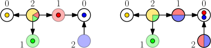
Figure 1: Example of the load balancing $2$-FLG. The clients (vertices) split their weight (shown by numbers) among the facilities (colored dots) in their shopping range. The client distributions are shown by colored pie charts. Left: The blue facility receives a load of $2$ while all other facilities get a load of $\frac{4}{3}$. The left client with weight $2$ distributes weight $\frac{4}{3}$ to the yellow facility and $\frac{1}{3}$ to both the green and the red facility. The state is not in SPE as the red facility can improve her load to $\frac{3}{2}$ by co-locating with the blue facility. Right: A SPE for this instance, all facilities have a load of $\frac{3}{2}$.

We define the stable states of the $2$-FLG as subgame perfect equilibria (SPE), since we inherently have a two-stage game. First, the facility agents select locations for their facilities and then, given this facility placement, the clients strategically distribute their spending capacity among the facilities in their shopping range. A state $(\mathbf{s},\sigma)$ is in SPE, or stable, if

• $\forall f_{j}\in\mathcal{F},\forall s_{j}^{\prime}\in V$: $\ell_{j}(\mathbf{s},\sigma)\geq\ell_{j}((s_{j}^{\prime},s_{-j}),\sigma)$ and

• $\forall\mathbf{s}\in\mathcal{S},\forall v_{i}\in V:L_{i}(\mathbf{s},\sigma)\leq L_{i}(\mathbf{s},(\sigma_{i}^{\prime},\sigma_{-i}))$ for all feasible weight distributions $\sigma^{\prime}(\mathbf{s},v_{i})$ of client $v_{i}$.

We say that client $v_{i}$ is covered by $\mathbf{s}$, if $N_{\mathbf{s}}(v_{i})\neq\emptyset$, and uncovered by $\mathbf{s}$, otherwise. Let $C(\mathbf{s})=\{v_{i}\mid v_{i}\in V,N_{\mathbf{s}}(v_{i})\neq\emptyset\}$ denote the set of covered clients under facility placement $\mathbf{s}$. We will compare states of the $2$-FLG by measuring their social welfare that is defined as the weighted participation rate $W(\mathbf{s})=w(C(\mathbf{s}))=\sum_{v_{i}\in C(\mathbf{s})}w(v_{i})$, i.e., the total spending capacity of all covered clients. For a host graph $H$ and a number of facility agents $k$, let $\text{\emph{OPT}}(H,k)$ denote the facility placement profile that maximizes the weighted participation rate $W(\text{\emph{OPT}}(H,k))$ among all facility placement profiles with $k$ facilities on host graph $H$.

We measure the inefficiency due to the selfishness of the agents via the Price of Anarchy (PoA) and the Price of Stability (PoS). Let $\text{bestSPE}(H,k)$ (resp. $\text{worstSPE}(H,k)$) denote the SPE with the highest (resp. lowest) social welfare among all SPEs for a given host graph $H$ and a facility number $k$. Moreover, let $\mathcal{H}$ be the set of all possible host graphs $H$. Then the PoA is defined as

$$PoA:=\max_{H\in\mathcal{H},k}W(\text{\emph{OPT}}(H,k))/W(\text{worstSPE}(H,k)),$$

whereas the PoS is defined as

$$PoS:=\max_{H\in\mathcal{H},k}W(\text{\emph{OPT}}(H,k))/W(\text{bestSPE}(H,k)).$$

We study dynamic properties of the $2$-FLG. Let an improving move by some (facility or client) agent be a strategy change that improves the agent’s utility. A game has the finite improvement property (FIP) if all sequences of improving moves are finite. The FIP is equivalent to the existence of an ordinal potential function Monderer and Shapley (1996).

1.3 Our Contribution

We introduce and analyze the $2$-FLG, a general model for competitive facility location games, where facility agents and also client agents act strategically. We focus on the load balancing $2$-FLG, where clients selfishly try to minimize their maximum waiting times that not only depend on the placement of the facilities but also on the behavior of all other client agents. We show that client equilibria always exist and that all client equilibria are equivalent from the facility agents’ point-of-view. Additionally, we provide an efficient algorithm for computing the facility loads in a client equilibrium that enables facility agents to efficiently anticipate the clients’ behavior. This is crucial in a two-stage game-theoretic setting. Moreover, since there are only $n$ possible locations for facilities, we can efficiently check if a given state of the load balancing $2$-FLG is in SPE. Using a potential function argument, we can show that a SPE always exists.

Finally, we consider the $2$-FLG with an arbitrary feasible client weight distribution function. For this broad class of games, we prove that the PoA is upper bounded by $2$ and we give an almost tight lower bound of $2-\frac{1}{k}$ on the PoA and PoS. This implies an almost tight PoA lower bound for the load balancing $2$-FLG. Furthermore, we show that computing a social optimum state for the $2$-FLG with an arbitrary feasible client weight distribution function $\sigma$ is NP-hard for all feasible $\sigma$, hence, also for the load balancing $2$-FLG.

2 Load Balancing Clients

In this section we analyze the load balancing $2$-FLG in which we consider not only strategic facilities that try to get patronized by as many clients as possible but we also have selfish clients that strategically distribute their spending capacity to minimize their maximum waiting time for getting serviced. We start with a crucial statement that enables the facility agents to anticipate the clients’ behavior.

Theorem 1.

For a facility placement profile $\mathbf{s}$, a client equilibrium $\sigma$ exists and every client equilibrium induces the same facility loads $(\ell_{1}(\mathbf{s},\sigma),\ldots,\ell_{k}(\mathbf{s},\sigma))$.

Proof.

We consider the following optimization problem (EQ):

$$\min_{\sigma}\sum_{i=1}^{k}\ell_{i}(\mathbf{s},\sigma)^{2}$$

subject to

$$\sigma(\mathbf{s},v_{i})_{j} \geq 0 \text{ for all }f_{j}\in N_{\mathbf{s}}(v_{i})$$

$$\sigma(\mathbf{s},v_{i})_{j} =0 \text{ for all }f_{j}\notin N_{\mathbf{s}}(v_{i})$$

$$\sum_{f_{j}\in N_{\mathbf{s}}(v_{i})}\sigma(\mathbf{s},v_{i})_{j} =w(v_{i}) \text{ if }N_{\mathbf{s}}(v_{i})\neq\emptyset$$

It is easy to see that an optimal solution $\sigma$ of EQ is a client equilibrium. For the sake of contradiction, assume that there exists a client $v_{i}$ and two facility agents $f_{p}$ and $f_{q}$ with $\ell_{q}(\mathbf{s},\sigma)>\ell_{p}(\mathbf{s},\sigma)$ and $\sigma(\mathbf{s},v_{i})_{q}>0$. However, this contradicts the optimality of $\sigma$ as the KKT conditions Peressini et al. (1988) demand that $\ell_{q}(\mathbf{s},\sigma)\leq\ell_{p}(\mathbf{s},\sigma)$ for all $f_{p},f_{q}\in N_{\mathbf{s}}(v_{i})$ with $\sigma(\mathbf{s},v_{i})_{q}>0$. Moreover, the KKT conditions are precisely the conditions of a client equilibrium, hence every equilibrium is an optimal solution of EQ.

Observe that the objective of EQ is convex in the facilities’ loads $\ell_{1}(\mathbf{s},\sigma),\ldots,\ell_{k}(\mathbf{s},\sigma)$ and the set of feasible solutions is compact and convex. Suppose there are two global optima $\sigma$ and $\sigma^{\prime}$ of EQ. By convexity of the objective function, we must have $\ell_{j}(\mathbf{s},\sigma)=\ell_{j}(\mathbf{s},\sigma^{\prime})$ for all facility agents $f_{j}$ as otherwise a convex combination of $\sigma$ and $\sigma^{\prime}$ would yield a feasible solution for EQ with smaller objective function value. ∎

Two facility agents sharing a client have equal load if the shared client puts weight on both of them:

Lemma 1.

In the load balancing $2$-FLG, for a facility placement $\mathbf{s}$, in a client equilibrium $\sigma$, if there are two facility agents $f_{p}$ and $f_{q}$ and a client $v_{i}$ with $p,q\in P_{i}(\mathbf{s},\sigma)$, then $\ell_{p}(\mathbf{s},\sigma)=\ell_{q}(\mathbf{s},\sigma)$.

Proof.

Let $v_{i}$ be a client and $p$ be the agent with the highest load in $P_{i}(\mathbf{s},\sigma)$. Assume that there is an agent $q\in P_{i}(\mathbf{s},\sigma)$ with $\ell_{p}(\mathbf{s},\sigma)>\ell_{q}(\mathbf{s},\sigma)$. In this case, the client $v_{i}$ decreases her weight on $f_{p}$ (and all facility agents in $P_{i}(\mathbf{s},\sigma)$ with the same load) and increases her weight on $f_{q}$, decreasing her total costs. This contradicts $\sigma$ being a client equilibrium. ∎

Next, we define a shared client set, which represents a set of facility agents who share weight of the same clients.

Definition 1.

For a facility placement profile $\mathbf{s}$, let $f_{p}$ be an agent, $\sigma$ be a client equilibrium. We define a shared client set of facility agents $S_{\sigma}(f_{p})$, such that (1) $f_{p}\in S_{\sigma}(f_{p})$ and (2) For two facility agents $f_{q},f_{r}$: If $f_{q}\in S_{\sigma}(f_{p})$ and there is a client $v_{i}$ with $q,r\in P_{i}(\mathbf{s},\sigma)$, then $f_{r}\in S_{\sigma}(f_{p})$.

We prove two properties of such a shared client set: First, all facility agents in a shared client set have the same load, and second, a client’s weight is either completely inside or completely outside a shared client set in a client equilibrium.

Lemma 2.

For a facility placement $\mathbf{s}$ in a client equilibrium $\sigma$, for every $f_{q},f_{r}\in S_{\sigma}(f_{p})$ we have $\ell_{q}(\mathbf{s},\sigma)=\ell_{r}(\mathbf{s},\sigma)$.

Proof.

As $f_{q}$ and $f_{r}$ are both members of $S_{\sigma}(f_{p})$ there exists a sequence of facility agents $F=(f_{q},f_{i_{1}},f_{i_{2}},\dots,f_{r})$, in which two adjacent facility agents share a client. By Lemma 1, each pair of neighbors in $F$ has identical loads. Thus, $\ell_{q}(\mathbf{s},\sigma)=\ell_{r}(\mathbf{s},\sigma)$. ∎

The next lemma follows from Definition 1:

Lemma 3.

For a facility placement $\mathbf{s}$, in a client equilibrium $\sigma$ for every client $v_{i}$ and facility agent $f_{p}$ with $p\in P_{i}(\mathbf{s},\sigma)$ , we have that for every facility agent $f_{r}\notin S_{\sigma}(f_{p})$ it holds that $r\notin P_{i}(\mathbf{s},\sigma)$.

Additionally, we show that each facility agent’s load can only take a limited number of values.

Lemma 4.

For a facility placement profile $\mathbf{s}$, in a client equilibrium $\sigma$ a facility agent’s load can only take a value of the form $\frac{x}{y}$ for $x\leq w_{\mathbf{s}}(\mathcal{F})$ and $y\leq k$ with $x,y\in\mathbb{N}$.

Proof.

If a client is shared between two facilities, these two facilities must, by Lemma 1, have the same load. We consider an arbitrary facility agent $f_{j}$ and her shared client set $S_{\sigma}(f_{j})$. All facility agents in $S_{\sigma}(f_{j})$ have the same load by Lemma 2 and all clients which have weight on a facility agent on $S_{\sigma}(f_{j})$ have their complete weight inside $S_{\sigma}(f_{j})$ by Lemma 3. Therefore, the sum of loads of the facility agents $S_{\sigma}(f_{j})$ must be an integer $i\leq w_{\mathbf{s}}(\mathcal{F})$. Thus, the load of $f_{j}$ is $\frac{i}{|S_{\sigma}(f_{j})|}$. Since $i\leq w_{\mathbf{s}}(\mathcal{F})$ (sum of client weights) and $|S_{\sigma}(f_{j})|\leq k$ (number of facility agents) with $i,|S_{\sigma}(f_{j})|\in\mathbb{N}$, the lemma is true. ∎

Definition 2.

For a facility placement profile $\mathbf{s}$, a set of facility agents $\emptyset\subset M\subseteq\mathcal{F}$ is a minimum neighborhood set (MNS) if for all $\emptyset\subset T\subseteq\mathcal{F}\text{:}\frac{w(A_{\mathbf{s}}(M))}{|M|}\leq\frac{w(A_{\mathbf{s}}(T))}{|T|}\text{.}$ We define the minimum neighborhood ratio (MNR) as $\rho_{\mathbf{s}}:=\frac{w(A_{\mathbf{s}}(M))}{|M|}\text{,}$ with $M$ being a MNS.

We show that a MNS receives the entire weight of all clients within its range and this weight is equally distributed.

Lemma 5.

For a facility placement profile $\mathbf{s}$, in a client equilibrium $\sigma$, each facility $f_{j}\in M$ of a minimum neighborhood set $M$ has a load of exactly $\ell_{j}(\mathbf{s},\sigma)=\rho_{\mathbf{s}}$.

Proof.

Let $M$ be a MNS and $\sigma$ be an arbitrary client equilibrium. Let $T=\operatorname*{arg\,min}_{f_{j}\in\mathcal{F}}{\left(\ell_{j}(\mathbf{s},\sigma)\right)}$ be the set of facility agents who share the lowest load in $\sigma$. Let $\ell_{T}$ be the load of each facility agents in $T$, hence for each $f_{j}\in T$ we have $\ell_{j}(\mathbf{s},\sigma)=\ell_{T}$. Assume for the sake of contradiction that $\ell_{T}<\frac{w(A_{\mathbf{s}}(M))}{|M|}$. Since $M$ is a MNS, we have

$$\frac{w(A_{\mathbf{s}}(T))}{|T|}\geq\frac{w(A_{\mathbf{s}}(M))}{|M|}\text{.}$$

Thus,

$$\sum_{f_{j}\in T}{\ell_{j}(\mathbf{s},\sigma)}=|T|\cdot\ell_{T} <|T|\frac{w(A_{\mathbf{s}}(M))}{|M|}$$

$$\leq|T|\frac{w(A_{\mathbf{s}}(T))}{|T|}=w(A_{\mathbf{s}}(T))\text{.}$$

Hence, there is at least one client agent $v_{i}$ in a range of at least one facility agent $f_{a}\in T$, who does not put her complete weight on the facility agents in $T$. Therefore, there is a facility agent $f_{b}\notin T$, with $\ell_{b}(\mathbf{s},\sigma)>\ell_{T}$ and $\sigma(\mathbf{s},v_{i})_{b}>0$. However, since $\ell_{b}(\mathbf{s},\sigma)>\ell_{T}$, $v_{i}$ would prefer to move weight away from $f_{b}$ to $f_{a}$. Thus, we arrive at a contradiction and in all client equilibria we have for each facility agent $f_{j}\in\mathcal{F}$ that $\ell_{j}(\mathbf{s},\sigma)\geq\frac{|A_{\mathbf{s}}(M)|}{|M|}$.

The facility agents in $M$ only have access to the clients in $A_{\mathbf{s}}(M)$. Thus, if for any facility agent $f_{c}\in M$ the utility is $\ell_{c}(\mathbf{s},\sigma)>\frac{w(A_{\mathbf{s}}(M))}{|M|}$, there must be another facility agent $f_{d}\in M$ where $\ell_{d}(\mathbf{s},\sigma)<\frac{w(A_{\mathbf{s}}(M))}{|M|}$ holds. Since this is not possible, we get for each facility agent $f_{j}\in M$ that $\ell_{j}(\mathbf{s},\sigma)=\frac{w(A_{\mathbf{s}}(M))}{|M|}$. ∎

2.1 Facility Loads in Polynomial Time

We present a polynomial-time combinatorial algorithm to compute the loads of the facility agents in a client equilibrium for a given facility placement profile $\mathbf{s}$. As each facility agent only has $n$ possible strategies, this implies that the best responses of facility agents are computable in polynomial time.

Algorithm 1 iteratively determines a MNS $M$, assigns to each facility in $M$ the MNR and removes the facilities and all client agents in their range from the instance. See Figure 2 for an example of a run of the algorithm.

1 if $\mathcal{F}=\emptyset$ then return ;

2 $M\leftarrow$ computeMNS($H,\mathcal{F},\mathbf{s}$);

3 for $f_{j}\in M$ do

4       $\ell_{j}(\mathbf{s},\sigma)\leftarrow\frac{w(A_{\mathbf{s}}(M))}{|M|}$;

5      

6$H^{\prime}\leftarrow(V,E,w^{\prime})$ with $w^{\prime}(v_{i})=0$ if $v_{i}\in A_{\mathbf{s}}(M)$ else $w^{\prime}(v_{i})=w(v_{i})$;

7 computeUtilities($H^{\prime},\mathcal{F}\setminus M,\mathbf{s}$);

Algorithm 1 computeUtilities($H=(V,E,w),\mathcal{F}$, $\mathbf{s}$)

Figure 2: An instance of the load balancing $2$-FLG with a facility placement profile marked by dots and $10$ clients with weight $1$ each. Algorithm 1 successively finds and removes the minimum neighborhood sets $S_{1}=\{f_{1}\}$, $S_{2}=\{f_{2},f_{3}\}$ and $S_{3}=\{f_{4}\}$.

The key ingredient of Algorithm 1 is the computation of a MNS in Algorithm 2.

1 construct directed graph $G=(V^{\prime},E_{st}\cup E_{\text{Range}})$;

2 $V^{\prime}\leftarrow\{s,t\}\cup V\cup\mathcal{F}$;

3 $E_{st}\leftarrow\{(s,v_{i},w(v_{i}))\mid v_{i}\in V\}\cup\{(f_{j},t,0)\mid f_{j}\in\mathcal{F}\}$;

4 $E_{\text{Range}}\leftarrow\{(v_{i},f_{j},w(v_{i}))\mid v_{i}\in V,f_{j}\in A_{\mathbf{s}}(v_{i})\}$;

5 possibleUtilities $\leftarrow$ sorted$(\{x/y\mid x,y\in\mathcal{N},0\leq x\leq w_{\mathbf{s}}(\mathcal{F}),1\leq y\leq k\})$;

6 for binary search over $i\in$ possibleUtilities do

7       $\forall{f_{j}\in\mathcal{F}}:$ capacity$((f_{j},t))\leftarrow i$;

8       $h\leftarrow$ maximum $s$-$t$-flow in $G$;

9       if $\text{value}(h)=i\cdot k$ then $i$ too small else $i$ too large;

10       

11$T\leftarrow\emptyset,\rho\leftarrow$ highest $i\in$ possibleUtilities below threshold;

12 for $f_{j}\in\mathcal{F}$ do

13       $\forall{f_{p}\in\mathcal{F}}:$ capacity$((f_{p},t))\leftarrow\rho$;

14       capacity$((f_{j},t))\leftarrow\infty$;

15       start with flow from binary search for $i=\rho$;

16       if $\nexists$ augmenting path in $G$ then

17             $T\leftarrow T\cup\{f_{j}\}$;

18            

19      

20return T;

Algorithm 2 computeMNS($H=(V,E,w),\mathcal{F},\mathbf{s}$)

Here, we first identify the MNR by a reduction to a maximum flow problem. To this end, we construct a graph, where from a common source vertex $s$ demand flows through the clients to the facility agents in their respective ranges and then to a common sink $t$. See Figure 3 for an example of such a reduction. By using binary search, we find the highest capacity value of the edges from the facility agents to the sink such that the flow can fully utilize all these edges. This capacity value is the value of the MNR $\rho_{\mathbf{s}}$. Note that by Lemma 4 the MNR can only attain a limited number of values. After determining the MNR, we identify the facility agents belonging to a MNS $M$ by individually increasing the capacity of the edge to the sink $t$ for each facility agent. Only if this does not increase the maximum flow, a facility agent belongs to $M$. By reusing the flow for $\rho_{\mathbf{s}}$ a search for an augmenting path with the increased capacity is sufficient to determine if the flow is increased.

Figure 3: Left: An instance of the load balancing $2$-FLG with the graph $H$ and the facility placement profile $\mathbf{s}$ marked by dots. Right: The maximum flow instance constructed by Algorithm 2.

We first prove the correctness of Algorithm 2:

Theorem 2.

For an instance of the load balancing $2$-FLG, a facility placement profile $\mathbf{s}$, Algorithm 2 computes a MNS.

Proof.

We show that the MNR $\rho$ computed by the algorithm is correct by proving that $\rho$ is a lower and upper bound for $\rho_{\mathbf{s}}$.

We show that for each set of facility agents $T$, we get $\rho\leq\frac{w(A_{\mathbf{s}}(T))}{|T|}$. To this end, consider the maximum flow for $i=\rho$. The value of this flow must be $\text{value}(h)=k\rho$, since $\rho$ is below the threshold found by the binary search. As the total capacity of the edges leaving the source $s$ towards vertices $v_{i}\in A_{\mathbf{s}}(T)$ is upper bounded by $w(A_{\mathbf{s}}(T))$ and every vertex $f_{p}$ with $f_{p}\in T$ is only reachable via vertices $v_{i}\in A_{\mathbf{s}}(T)$, the total inflow to the vertices $f_{p}\in T$ is $w(A_{\mathbf{s}}(T))$. Furthermore, the capacity of each edge from a facility vertex to the sink vertex $t$ is exactly $\rho$, hence each of these edges carries a flow of exactly $\rho$. Thus, we get $|T|\rho\leq w(A_{\mathbf{s}}(T))$ for every set of facility agents $T$.

For the upper bound, we show that there is a set $T$ for which $\rho\geq\frac{w(A_{\mathbf{s}}(T))}{|T|}$. We consider the flow at $i=\rho+\delta$, the value immediately above $\rho$ in possibleUtilities. We assume that for each set $T$, $\rho+\delta\leq\frac{w(A_{\mathbf{s}}(T))}{|T|}$. By Lemma 5, there must be a weight distribution $\sigma$, such that every facility agent receives $\rho+\delta$ load. Thus, setting the flow of every edge $(v_{i},f_{j})$ in $h$ to $\sigma(\mathbf{s},v_{i})_{j}$ for each $v_{i}\in V,f_{j}\in\mathcal{F}$ results in a flow of $(\rho+\delta)k$. This leads to $\rho+\delta$ being below the threshold and, hence, we have a contradiction. Therefore, there must be a set of facility agents $T$ with $\rho+\delta>\frac{w(A_{\mathbf{s}}(T))}{|T|}$. By Lemma 4, there is no value in between $\rho$ and $\rho+\delta$, which $\frac{w(A_{\mathbf{s}}(T))}{|T|}$ can attain. Thus, there must be a set $T$ with $\rho\geq\frac{w(A_{\mathbf{s}}(T))}{|T|}$.

It remains to show that the set of facility agents $M$ computed by the algorithm is indeed a MNS. By the feasibility of the total flow of $k\cdot\rho$ for the instance with capacity bounds of $\rho$, we have have for every set of facility agents $T$, $\frac{w(A_{\mathbf{s}}(T))}{|T|}\geq\rho$. For every $f_{j}\notin M$, there exists an augmenting path where the edge $(f_{j},t)$ has capacity $\infty$. Hence, there is a total flow strictly larger than $k\cdot\rho$ with flow of exactly $\rho$ through all $f_{q}\neq f_{j}$. As the flow through each $f_{i}$ is bounded by $w(A_{\mathbf{s}}(f_{i}))$, for every $T$ with $f_{j}\in T$, $\frac{w(A_{\mathbf{s}}(T))}{|T|}>\rho$. Therefore, $f_{j}$ does not belong to the MNS.

For every $f_{j}\in M$, the absence of an augmenting path certifies that the flow is constrained by capacity representing the clients’ spending capacities. Hence, $\frac{w(A_{\mathbf{s}}(T))}{|T|}=\rho$ for every $T\subseteq M$. ∎

With that, we bound the runtime of Algorithm 2.

Lemma 6.

Algorithm 2 runs in $\mathcal{O}(\log(w_{\mathbf{s}}(\mathcal{F})k)nk(n+k))$.

Proof.

Since $|\text{possibleUtilities}|\leq w_{\mathbf{s}}(\mathcal{F})k$, the binary search needs $\log{w_{\mathbf{s}}(\mathcal{F})k}$ steps. In each iteration, the dominant part is the computation of the flow, since all other operations are executable in constant time or are linear iterations through $G$. Therefore, the runtime of the binary search is the runtime of $\log{w_{\mathbf{s}}(\mathcal{F})k}$ flow computations in $G$. For the loop, we need $k$ breadth-first searches to determine the existence of augmenting paths.

The graph $G$ we create has $|V^{\prime}|=n+k+2$ vertices and at most $|E^{\prime}|\leq n+k+nk$ edges. These values are not changed throughout the algorithm. Thus, by using Orlin’s algorithm Orlin (2013), to compute the maximum flow in $\mathcal{O}(nk(n+k))$, which dominates the complexity of the loop and its augmenting path searches. Therefore, the algorithm runs in $\mathcal{O}(\log(w_{\mathbf{s}}(\mathcal{F})k)nk(n+k))$. ∎

We return to Algorithm 1 and prove correctness and runtime:

Theorem 3.

Given a facility placement profile $\mathbf{s}$, Algorithm 1 computes the agent loads for an instance of the load balancing $2$-FLG in $\mathcal{O}(\log(w_{\mathbf{s}}(\mathcal{F})k)nk^{2}(n+k))$.

Proof.

Correctness: By Lemma 5 the utilities determined for the client agents in the MNS $M$ are correct for the given instance. Also by Lemma 5, the client equilibria of $\mathcal{F}\setminus M$ are independent of the facility agents in $M$ and the clients in $A_{\mathbf{s}}(M)$. Therefore, we can remove $M$, set the weight of each client $v_{i}\in A_{\mathbf{s}}(M)$ to $w(v_{i})=0$ and proceed recursively.

Runtime: The recursive function is called at most $k$ times because the instance size is decreased by at least one facility agent in each iteration. Apart from the call to Algorithm 2, all computations can be done in constant or linear time. Therefore, the algorithm runs in $\mathcal{O}(\log(w_{\mathbf{s}}(\mathcal{F})k)nk^{2}(n+k))$. ∎

Algorithm 2 implicitly computes a client equilibrium.

Corollary 1.

A client equilibrium can be constructed by using the flow values on the edges between a client and the facility agents of the MNSs computed during the binary search in Algorithm 2 as the corresponding client weight distribution.

Proof.

Let $\mathbf{s}$ be a facility placement profile and for each facility $f_{j}$ let $h_{j}$ be the maximum $s$-$t$-flow found by the binary search during the run of Algorithm 2, which finds $f_{j}$ to be part of a MNS. We construct a client weight distribution $\sigma$ in the following way: For each pair $v_{i},f_{j}$, we set $\sigma(\mathbf{s},v_{i})_{j}=h_{j}(v_{i},f_{j})$, i.e., equal to the flow between $v_{i}$ and $f_{j}$ in $h_{j}$.

We now show that $\sigma$ is indeed a client equilibrium: Let $v_{i}$ be an arbitrary client. The algorithm removes her from the instance (i.e., sets her weight to 0) in the first round of Algorithm 1, where she has any facility $f_{p}$ of the MNS $M$ found in that round in her shopping range. Thus, all facilities $f_{j}$ with $\sigma(\mathbf{s},v_{i})_{j}>0$ are part of $M$. By the limit on the outgoing capacity of these facilities in the binary search in Algorithm 2, all facilities in $M$ have equal load in $\sigma$. Since the MNR is nondecreasing throughout the run of the algorithm, all facilities which are part of an MNS found in a later iteration, have a equal or higher load in $\sigma$ than the facilities in $M$. Therefore, client $v_{i}$ cannot improve by moving her weight. ∎

2.2 Existence of Subgame Perfect Equilibria

We show that the load balancing $2$-FLG always possesses SPE using a lexicographical potential function. For that, we show that when a facility agent $f_{p}$ changes her strategy, no other facility agent $f_{q}$’s load decreases below $f_{p}$’s new load.

Lemma 7.

Let $\mathbf{s}$ be a facility placement profile and $f_{p}$ a facility agent with an improving move $s^{\prime}_{p}$ such that $\ell_{p}((s^{\prime}_{p},s_{-p}),\sigma^{\prime})>\ell_{p}(\mathbf{s},\sigma)$, where $\sigma,\sigma^{\prime}$ are client equilibria. For every facility agent $f_{q}$ with $\ell_{q}((s^{\prime}_{p},s_{-p}),\sigma^{\prime})<\ell_{q}(\mathbf{s},\sigma)$, we have that $\ell_{q}((s^{\prime}_{p},s_{-p}),\sigma^{\prime})\geq\ell_{p}((s^{\prime}_{p},s_{-p}),\sigma^{\prime})$.

Proof.

Let $Q$ be the set of facility agents $f_{q}$ with $\ell_{q}((s^{\prime}_{p},s_{-p}),\sigma^{\prime})<\ell_{q}(\mathbf{s},\sigma)$. Let $Q_{\text{min}}=\operatorname*{arg\,min}_{q\in Q}\{\ell_{q}((s^{\prime}_{p},s_{-p}),\sigma^{\prime})\}$. Now, we distinguish two cases for $f_{p}$:

Case 1: $f_{p}\in Q_{\text{min}}$. The statement is trivially true.

Case 2: $f_{p}\notin Q_{\text{min}}$. All facility agents in $Q_{\text{min}}$ have the same clients in their ranges as before. Thus, there must be a client $v_{i}$, who has decreased her weight on a facility agent $f_{r}\in Q_{\text{min}}$ and increased her weight on a facility agent $f_{s}\notin Q_{\text{min}}$. Hence, we have $\ell_{s}((s^{\prime}_{p},s_{-p}),\sigma^{\prime})\leq\ell_{r}(\mathbf{s},\sigma)$ as otherwise, the client $v_{i}$ would not put weight on $f_{s}$. We assume $f_{p}\not=f_{s}$. As $\sigma$ is a client equilibrium, we have that $\ell_{r}(\mathbf{s},\sigma)\leq\ell_{s}(\mathbf{s},\sigma)$. This implies $\ell_{s}((s^{\prime}_{p},s_{-p}),\sigma^{\prime})<\ell_{s}(\mathbf{s},\sigma)$ which contradicts $f_{s}\notin Q_{\text{min}}$. Therefore, $f_{p}=f_{s}$ and $\ell_{r}((s^{\prime}_{p},s_{-p}),\sigma^{\prime})\geq\ell_{p}((s^{\prime}_{p},s_{-p}),\sigma^{\prime})$, which means that for each facility agent $f_{q}\in Q$, it holds that $\ell_{q}((s^{\prime}_{p},s_{-p}),\sigma^{\prime})\geq\ell_{p}((s^{\prime}_{p},s_{-p}),\sigma^{\prime})$. ∎

With this lemma, we prove the FIP and, hence, existence of a SPE by a lexicographic potential function argument.

Theorem 4.

The load balancing $2$-FLG has the FIP.

Proof.

Let $\Phi(\mathbf{s})\in\mathbb{R}^{k}$ be the vector that lists the loads $\{\ell_{1}(\mathbf{s},\sigma),$ $\ell_{2}(\mathbf{s},\sigma),\dots,\ell_{k}(\mathbf{s},\sigma)\}$ in an increasing order.

Let $\mathbf{s}$ be a facility placement profile and $f_{p}$ a facility agent with an improving move $s^{\prime}_{p}$ such that $\ell_{p}((s^{\prime}_{p},s_{-p}),\sigma^{\prime})>\ell_{p}(\mathbf{s},\sigma)$, where $\sigma,\sigma^{\prime}$ are client equilibria. We show that $\Phi(s^{\prime}_{p},s_{-i})<_{\text{lex}}\Phi(\mathbf{s})$. Let $\Phi(\mathbf{s})$ be of the form $\Phi(\mathbf{s})=(\phi_{1},\ldots,\phi_{\alpha},\ell_{p}(\mathbf{s},\sigma),\phi_{\alpha+1},\ldots,\phi_{\beta},$ $\phi_{\beta+1},\ldots,\phi_{k-1})\text{,}$ for some $\alpha\leq\beta\leq k-1$, such that for every $1\leq j\leq\beta$: $\phi_{j}<\ell_{p}((s^{\prime}_{p},s_{-p}),\sigma^{\prime})$ and for every $j\geq\beta+1:\phi_{j}\geq\ell_{p}((s^{\prime}_{p},s_{-p}),\sigma^{\prime})$.

By Lemma 7, we have for all facility agents $f_{q}$ with a load $\ell_{q}(\mathbf{s},\sigma)\in\{\phi_{1},\ldots,\phi_{\beta})$ that their loads did not decrease. and for agents $f_{q}$ with $\ell_{q}(\mathbf{s},\sigma)\in\{\phi_{\beta+1},\ldots,\phi_{k})$ we have $\ell_{q}((s^{\prime}_{p},s_{-p}),\sigma^{\prime})\geq\ell_{p}((s^{\prime}_{p},s_{-p}),\sigma^{\prime})$. With the improvement of $f_{p}$, $\Phi(s^{\prime}_{p},s_{-p})>_{\text{lex}}\Phi(\mathbf{s})$ holds. By Lemma 4, there is a finite set of values that the loads can attain, thus, $\Phi$ is an ordinal potential function and the game has the FIP. ∎

3 Comparison with Utility Systems

A utility system (US) Vetta (2002) is a game, in which agents gain utility by selecting a set of actions, which they choose from a collection of subsets of a groundset available to them. Utility is assigned to the agents by a function of the set of selected actions of all agents.

Definition 3 (Utility Systems (US)  Vetta (2002)).

A utility systems consists of a set of $k$ agents, a groundset $V_{p}$ for each agent $p$, a strategy set of feasible action sets $\mathcal{A}_{p}\subseteq 2^{V_{p}}$, a social welfare function $\gamma:2^{V^{*}}\to\mathbb{R}$ and a utility function $\alpha_{p}:2^{V^{*}}\to\mathbb{R}$ for each player $p$, where $V^{*}=\cup_{p\in P}{V_{p}}$.

For a strategy vector $(a_{1},\dots,a_{k})$, let $A=a_{1}\cup\dots\cup a_{k}$ and $A\oplus a_{p}^{\prime}$ denotes the set of actions obtained if player $p$ changes her action set from $a_{p}$ to $a_{p}^{\prime}$. A game is a utility system if $\alpha_{p}(A)\geq\gamma(A\oplus\emptyset)\text{.}$ The utility system is basic if $\alpha_{p}(A)=\gamma(A\oplus\emptyset)$ and is valid if $\sum_{p\in P}{\alpha_{p}(A)}\leq\gamma(a)\text{.}$

We show that the load balancing $2$-FLG is not a basic but a valid US and we can apply the corresponding bounds for the PoA but not the existence of stable states.

Lemma 8.

The load balancing $2$-FLG is a US.

Proof.

Each facility agent $f_{p}$ corresponds to a player $p$ in the US with the groundset $V_{p}=\{v^{p}\mid\text{ for each }v\in V\}$ and the action set $\mathcal{A}_{p}=\{\{v^{p}\}\cup\{w^{p}\in V\mid(v,w)\in E\}\mid v\in V\}$. We can define $\gamma(X)=\sum_{v\in V\mid\exists p:v^{p}\in X}{w(v)}\text{,}$ which corresponds to the sum of weights of covered clients and $\alpha_{p}(A)$ to correspond to the load of $f_{p}$ which can be expressed as a function of the sets of clients in range of each facility. To show the US condition $\alpha_{p}(A)\geq\gamma(A\oplus\emptyset)$, we let the social welfare decrease by a value of $x$ through a removal of player $p$ from strategy profile $a$ resulting in a new strategy profile $a_{-p}$. Hence, clients with a total weight of $x$ were only covered by $p$ in $a$. Thus, player $p$ must receive at least $x$ utility in $a$, and the condition is fulfilled. ∎

As $\gamma$ merely depends on the covered clients, we have for every $X,Y\subset V^{*}$ with $X\subseteq Y$ and any $v^{p}\in V^{*}\setminus Y$, we have that $\gamma(X\cup\{v^{p}\})-\gamma(X)\geq\gamma(X\cup\{v^{p}\})-\gamma(X)$. Hence, the following lemma is immediate.

Lemma 9.

The function $\gamma$ is non-decreasing and submodular.

We now show that the load balancing $2$-FLG is a valid but not basic US.

Theorem 5.

The load balancing $2$-FLG is a valid, but not a basic US.

Proof.

The following example proves that the load balancing $2$-FLG is not a basic US . Let $H=(V,E,w)$ with $V=(v_{1},v_{2})$, $w(v_{1})=w(v_{2})=1$ and $E=\{(v_{1},v_{2}),(v_{2},v_{1})\}$. Furthermore, we have two facility players $f_{p}$ and $f_{q}$ with $\mathbf{s}=(v_{1},v_{2})$. Removing player $f_{p}$ does not change the weighted participation rate $W(\mathbf{s})$ since all clients are still covered. However, the utility of the removed facility player $f_{p}$ is equal to $1$. Hence, equality in the utility system condition does not hold and the US is not basic.

To show that the load balancing $2$-FLG is a valid US, note that each client $v$ who is in the attraction range of at least one facility player distributes her total weight $w(v)$ among the players. All other clients are uncovered and hence, their distributed weight is equal to $0$. Thus, the total weight $\sum_{v_{i}\in C(\mathbf{s})}w(v_{i})$ distributed by clients, which is equal to the sum of the facility players’ loads, is equal to the value of the welfare function $W(\mathbf{s})$. ∎

We are now able to apply the PoA bound of Vetta (2002) to our model.

Corollary 2.

The PoA of the load balancing $2$-FLG is at most 2.

4 Arbitrary Client Behavior

In the following, we investigate the quality of stable states of the $2$-FLG with arbitrary client behavior, i.e., the client costs are arbitrarily defined, and provide an upper and lower bound for the PoA as well as a lower bound for the PoS. Additionally, we show that computing the social optimum is NP-hard.

Theorem 6.

The PoA of the $2$-FLG is at most $2$.

Proof.

Fix a $2$-FLG with $k$ facility players. Let OPT be a facility placement profile that maximizes social welfare and let $(SPE,\sigma_{\text{SPE}})$ be a SPE. Let $C(\text{SPE})$ be the set of clients $v_{i}$ which are covered in SPE and $C(\text{OPT})$ be the set of clients $v_{i}$ which are covered in OPT, respectively. Let UNCOV $=C(\text{OPT})\setminus C(\text{SPE})$ be the set of clients which are covered in OPT but uncovered in SPE.

Assume that $W(\text{OPT})>2W(\text{SPE})$ and hence, $\sum_{v\in\text{UNCOV}}w(v)>W(\text{SPE})$. Then, there exists a facility player $f_{p}$ that receives in OPT more than $\frac{W(\text{SPE})}{k}$ load from the clients in UNCOV. Now consider a facility agent $f_{q}$ with load $\ell_{q}\left(\text{SPE},\sigma_{\text{SPE}}\right)\leq\frac{W(\text{SPE})}{k}$. By changing her strategy and selecting the position of facility agent $f_{p}$ in OPT, agent $f_{q}$ receives the weight of all clients in UNCOV which are covered by $f_{p}$ in OPT since they are currently uncovered and therefore, obtains more than $\frac{W(\text{SPE})}{k}$ load. As this contradicts the assumption of $\left(\text{SPE},\sigma_{\text{SPE}}\right)$ being a SPE, we have that $W(\text{OPT})\leq 2W(\text{SPE})$. ∎

We contrast the upper bound of the PoA with a lower bound for the PoA and PoS.

Theorem 7.

The PoA and PoS of the $2$-FLG is at least $2-\frac{1}{k}$.

Proof.

We prove the statement by providing an example of an instance I which has a unique equilibrium. Let $x\geq 4$, $x\in\mathbb{N}$. We construct a $2$-FLG with $k$ facility players, a host graph $H(V,E,w)$ with $V=\{v_{1},\ldots,v_{k},$ $v_{1,1},\ldots,v_{1,x-1},$ $v_{2,1},$ $\ldots,v_{k-1,x-1},v_{k,1},\ldots,v_{k,kx}\}$, for all $v\in V$, $w(v)=1$ and $E=\{(v_{i},v_{i,j})\mid i\in[1,k-1],j\in[1,x-1]\}\ \cup\{(v_{k},v_{k,i})\mid i\in[1,kx]\}\ \cup\{(v_{k,i},v_{i,1})\mid i\in[1,k-1]\}$. See Figure 4.

Figure 4: The host graph $H$ of an instance $I$ of the $2$-FLG with arbitrary client behavior with a unique SPE.

We note that $H$ consists of a large star $S_{k}$ with central vertex $v_{k}$, leaf vertices $(v_{k,1},\ldots,v_{k,kx})$ and $k-1$ small stars $S_{i}$ for $i\in[1,k-1]$ with central vertices $v_{i}$ and leaf vertices $(v_{i,1},\ldots,v_{i,x-1})$. Each star $S_{i}$ is connected to $S_{k}$ via an edge between a leaf vertex of $S_{k}$ and $S_{i}$, i.e., $(v_{k,i},v_{i,1})$.

If the $k$ facility players are placed on $\mathbf{s}_{\text{OPT}}=(v_{1},\ldots,v_{k})$, all clients are covered by exactly one facility. Hence, $W(OPT(H,k))=|V|=kx+k+(k-1)(x-1)$.

In any equilibrium, a facility $f_{j}$ for $j\in[1,k]$ must receive a load of at least $\frac{kx+1}{k}=x+\frac{1}{k}$ as otherwise switching to vertex $v_{k}$ with $kx+1$ adjacent vertices yields an improvement. However, any other vertex in $H$ has at most $x-1$ adjacent vertices, hence, every facility player gets a load of at most $x$. Therefore, the unique $SPE$ is $\mathbf{s}_{\text{SPE}}=(v_{k},\ldots,v_{k})$ with $W(\mathbf{s}_{\text{SPE}})=kx+1$ and $PoA=PoS=\frac{kx+k+(k-1)(x-1)}{kx+1}=\frac{(2k-1)x+1}{kx+1}$. We get $\lim\limits_{x\rightarrow\infty}\left(\frac{(2k-1)x+1}{kx+1}\right)=\frac{2k-1}{k}=2-\frac{1}{k}.$ ∎

By a reduction from 3SAT, we show that computing OPT$(H,k)$ is an NP-hard problem.

Theorem 8.

Given a host graph $H$ and a number of $k$ facilities, computing the facility placement maximizing the weighted participation rate OPT$(H,k)$, is NP-hard.

Proof.

We prove the theorem by giving a polynomial time reduction from the NP-hard 3SAT problem.

For a 3SAT instance $\phi$ with a set of clauses $C$ and a set of variables $X$, we create a $2$-FLG instance with $k=|X|$ facility players where the host graph $H(V_{X}\cup V_{C},E_{X}\cup E_{C},w)$ is defined as follows:

$$w(v) =\{1\mid v\in V_{X}\cup V_{C}\}$$

$$V_{X} =\{v_{x},v_{\neg x}\mid x\in X\}$$

$$V_{C} =\{v_{c}\mid c\in C\}\}$$

$$E_{X} =\{(v_{x},v_{\neg x}),(v_{\neg x},v_{x})\mid x\in X\}$$

$$E_{C} =\{(v_{c},v_{l})\mid c\in C,\text{ literal }l\in c\},$$

where $v_{l}=v_{x}$ if the contained variable $x$ is used as a true literal in $c$, and $v_{l}=v_{\neg x}$, otherwise. See Figure 5 for an example.

Figure 5: An example of a corresponding host graph $H$ to the 3SAT instance ${(x\vee\neg y\vee z)}\wedge{(\neg x\vee y\vee z)}$.

Let $\phi$ be satisfiable and $\alpha$ be an assignment of the variables satisfying $\phi$. We set $\mathbf{s}=(s_{1},\ldots,s_{k})$ such that for $i\in[1,k]$, $x_{i}\in X$, $s_{i}=v_{x_{i}}$ if $x_{i}$ is true in $\alpha$ and $s_{i}=v_{\neg x_{i}}$ otherwise. By $E_{X}$, $v_{x_{i}}$ and $v_{\neg x_{i}}$ are covered by a facility player either located on $v_{x_{i}}$ or $v_{\neg x_{i}}$. To show that each client $v_{c}\in V_{C}$ is covered as well, consider the corresponding clause $c=l_{1}\vee l_{2}\vee l_{3}$. Since $\phi$ is satisfied, at least one of the literals is true, which means that at least one of $v_{l_{1}}$, $v_{l_{2}}$ and $v_{l_{3}}$ must be occupied by a facility in $\mathbf{s}$. Thus, if $\phi$ is satisfied, we get a placement where all clients are covered, which is optimal.

Let $\mathbf{s}$ be a facility placement profile where all clients are covered. Note that this implies that for each $x\in X$ either $v_{x},v_{\neg x}$ is occupied by a facility player. Hence, all facilities are placed on vertices in $V_{X}$. We construct an assignment of the variables $\alpha$ as follows: $x=$ true, if $v_{x}\in\mathbf{s}$ and $x=$ false, if $v_{\neg x}\in\mathbf{s}$. Let $c\in C$ be an arbitrary clause in $\phi$. The corresponding vertices $v_{c}$ is covered by a facility player which is placed on an adjacent vertex, $v_{l_{1}}$, $v_{l_{2}}$, or $v_{l_{3}}$. This implies that at least one of the literals $l_{1}$, $l_{2}$, and $l_{3}$ is true in $\alpha$ and therefore $c$ is satisfied. Hence, $\phi$ is satisfiable. ∎

5 Conclusion and Future Work

We provide a general model for non-cooperative facility location with both strategic facilities and clients. Our load balancing $2$-FLG is a proof-of-concept that even in this more intricate setting it is possible to efficiently compute and check client equilibria. Also, in contrast to classical one-sided models and in contrast to Kohlberg’s two-sided model, the load-balancing $2$-FLG has the favorable property that stable states always exist and that they can be found via improving response dynamics. Moreover, our bounds on the PoA and the PoS show that the broad class of 2-FLGs is very well-behaved since the societal impact of selfishness is limited.

The load balancing $2$-FLG is only one possible realistic instance of a competitive facility location model with strategic clients; other objective functions are conceivable, e.g., depending on the distance and the load of all facilities in their shopping range. Also, besides the weighted participation rate other natural choices for the social welfare function are possible, e.g., the total facility variety of the clients, i.e., for each client, we count the facilities in her shopping range. This measures how many shopping options the clients have. Moreover, we are not aware that the total facility variety has been considered for any other competitive facility location model.

References

- Ahn et al. [2004] Hee-Kap Ahn, Siu-Weng Cheng, Otfried Cheong, Mordecai Golin, and René van Oostrum. Competitive Facility Location: The Voronoi Game. TCS, 310(1):457 – 467, 2004.
- Anshelevich et al. [2004] Elliot Anshelevich, Anirban Dasgupta, Jon Kleinberg, Éva. Tardos, Tom Wexler, and Tim Roughgarden. The Price of Stability for Network Design with Fair Cost Allocation. In FOCS, pages 295–304, 2004.
- Boppana et al. [2016] Meena Boppana, Rani Hod, Michael Mitzenmacher, and Tom Morgan. Voronoi Choice Games. In ICALP, volume 55, pages 23:1–23:13, 2016.
- Brethouwer et al. [2018] Jan-Tino Brethouwer, Jasper de Jong, Marc Jochen Uetz, and Alexander Skopalik. Analysis of Equilibria for Generalized Market Sharing Games. In WINE, 2018.
- Cohen and Peleg [2019] Avi Cohen and David Peleg. Hotelling Games with Random Tolerance Intervals. In WINE, pages 114–128, 2019.
- de Berg et al. [2019] Mark de Berg, Sándor Kisfaludi-Bak, and Mehran Mehr. On One-Round Discrete Voronoi Games. In ISAAC, volume 149, pages 37:1–37:17, 2019.
- Downs [1957] Anthony Downs. An Economic Theory of Political Action in a Democracy. Journal of Political Economy, 65(2):135–150, 1957.
- Dürr and Thang [2007] Christoph Dürr and Nguyeb Kim Thang. Nash Equilibria in Voronoi Games on Graphs. In ESA, pages 17–28, 2007.
- Eiselt et al. [1993] Horst A. Eiselt, Gilbert Laporte, and Jaques-Francois Thisse. Competitive Location Models: A Framework and Bibliography. Transportation Science, 27(1):44–54, 1993.
- Feldman et al. [2016] Michal Feldman, Amos Fiat, and Svetlana Obraztsova. Variations on the Hotelling-Downs Model. In AAAI, pages 496–501, 2016.
- Feldotto et al. [2019] Matthias Feldotto, Pascal Lenzner, Louise Molitor, and Alexander Skopalik. From Hotelling to Load Balancing: Approximation and the Principle of Minimum Differentiation. In AAMAS, pages 1949–1951, 2019.
- Fournier et al. [2020] Gaëtan Fournier, Karine Van der Straeten, and Jörgen Weibull. Spatial Competition with Unit-Demand Functions. TSE Working Papers 20-1072, 2020.
- Gairing [2009] Martin Gairing. Covering Games: Approximation through Non-Cooperation. In WINE, pages 184–195, 2009.
- Goemans et al. [2006] Michel Goemans, Erran Li Li, Vehab S. Mirrokni, and Marina Thottan. Market Sharing Games Applied to Content Distribution in Ad hoc Networks. Journal on Selected Areas in Communications, 24(5):1020–1033, 2006.
- Gur et al. [2018] Yonatan Gur, Daniel Saban, and Nicolas E. Stier-Moses. The Competitive Facility Location Problem in a Duopoly: Advances Beyond Trees. Operations Research, 66(4):1058–1067, 2018.
- Hotelling [1929] Harold Hotelling. Stability in Competition. The Economic Journal, 39(153):41–57, 1929.
- Kohlberg [1983] Elon Kohlberg. Equilibrium Store Locations When Consumers Minimize Travel Time Plus Waiting Time. Economics Letters, 11(3):211 – 216, 1983.
- Koutsoupias and Papadimitriou [1999] Elias Koutsoupias and Christos Papadimitriou. Worst-Case Equilibria. In STACS, pages 404–413, 1999.
- Mavronicolas et al. [2008] Marios Mavronicolas, Burkhard Monien, Vicky G. Papadopoulou, and Florian Schoppmann. Voronoi Games on Cycle Graphs. In MFCS, pages 503–514, 2008.
- Monderer and Shapley [1996] Dov Monderer and Lloyd S. Shapley. Potential Games. Games and Economic Behavior, 14(1):124 – 143, 1996.
- Orlin [2013] James B. Orlin. Max flows in o(nm) time, or better. In Proceedings of the Forty-Fifth Annual ACM Symposium on Theory of Computing (STOC 2013), pages 765–774, 2013.
- Peressini et al. [1988] Anthony L. Peressini, Francis E. Sullivan, and Jerry J. Uhl. The Mathematics of Nonlinear Programming. Springer-Verlag New York, 1988.
- Peters et al. [2018] Hans Peters, Marc Schröder, and Dries Vermeulen. Hotelling’s Location Model with Negative Network Externalities. International Journal on Game Theory, 2018.
- Prisner [2011] Erich Prisner. Best Response Digraphs for Two Location Games on Graphs. Contributions to Game Theory and Management, 4(0):378–388, 2011.
- ReVelle and Eiselt [2005] Charles S. ReVelle and Horst A. Eiselt. Location Analysis: A Synthesis and Survey. European Journal of Operational Research, 165(1):1–19, 2005.
- Schmand et al. [2019] Daniel Schmand, Marc Schröder, and Alexander Skopalik. Network Investment Games with Wardrop Followers. In ICALP, volume 132, pages 151:1–151:14, 2019.
- Shen and Wang [2017] Weiran Shen and Zihe Wang. Hotelling-Downs Model with Limited Attraction. In AAMAS, pages 660–668, 2017.
- Teramoto et al. [2006] Sachio Teramoto, Erik D. Demaine, and Ryuhei Uehara. Voronoi Game on Graphs and its Complexity. In CIG, pages 265–271, 2006.
- Vetta [2002] Adrian Vetta. Nash Equilibria in Competitive Societies, with Applications to Facility Location, Traffic Routing and Auctions. FOCS, pages 416–425, 2002.