Density-functional approach to the band gaps of finite and periodic two-dimensional systems
Abstract
We present an approach based on density-functional theory for the calculation of fundamental gaps of both finite and periodic two-dimensional (2D) electronic systems. The computational cost of our approach is comparable to that of total energy calculations performed via standard semi-local forms. We achieve this by replacing the 2D local density approximation with a more sophisticated – yet computationally simple – orbital-dependent modeling of the exchange potential within the procedure by Guandalini et al. [Phys. Rev. B 99, 125140 (2019)]. We showcase promising results for semiconductor 2D quantum dots and artificial graphene systems, where the band structure can be tuned through, e.g., Kekulé distortion.
I Introduction
During the past decades, the ability to produce two-dimensional (2D) electron gas has led to the discovery of new physical phenomena and applications, including integer and fractional quantum Hall effect, semiconductor nanodevices such as quantum dots, and a variety of topological quantum systems [1]. On the other hand, the discoveries of atomic 2D materials, such as graphene, have inspired band-structure engineering in a variety of 2D systems [2, 3, 4, 5, 6, 7, 8, 9, 10, 11]. In addition, the recently discovered properties of twisted bilayer graphene [12, 13, 14] have led to next phase of so-called designer materials [15, 16, 17, 18, 19, 20, 21].
Density-functional theory (DFT) can provide a practical yet sufficiently accurate approach to compute the electronic structure of 3D materials and quantum confined low-dimensional systems [22]. The reliability of the results depends on the choice to approximate the exchange-correlation (xc) energy functional [23, 24, 25], which accounts for the many-body effects beyond the (classical) Hartree interaction. To examine 2D systems, the standard reference to the 3D electron gas used to derived approximate semi-local functional forms for atoms, molecules, and solids must be replaced by the 2D electron gas. Although numerous forms have been derived by now for 2D systems, [26, 27, 28, 29, 30, 31, 32, 33, 34, 35, 36, 37, 38, 39, 40, 41, 42, 43, 44] the computation of band gaps sets additional, non-trivial, challenges.
From the experience on 3D materials, it is known that standard semi-local DFT approximations (DFAs) often underestimate the actual band gaps, because they miss a crucial discontinuous shift in the xc potential. Accurate band gaps can be obtained from advanced many-body approximations such as GW calculations [45, 46, 47, 48], or by using orbital-dependent DFT functionals, e.g., hybrids [49, 50, 51, 52, 53, 54]. However, these approaches are computationally demanding. Further progress can be made by upgrading semi-local DFAs to consistent ensemble-DFT (EDFT) forms [55, 56, 57, 58], by switching to a recently introduced “N-centered” EDFT [59, 60, 61], or via non-variational models of the xc potential which can balance simplicity and accuracy [62, 63, 64, 65, 66, 67, 68, 69, 70, 71, 72, 73, 74]. The latter option is the thread that we follow here.
In this work, we extend the approach presented in Ref. 75 – which focused on finite systems – to compute the fundamental gaps of both finite and periodic 2D systems. We keep the computational cost restricted at about the level of a ground-state calculation performed by means of a standard semi-local approximation, then followed by an additional iteration at almost no extra cost. As a key step beyond what done in Ref. 75, we “transfer” the GLLB model potential by Gritsenko et al. [62] and its modifications by Kuisma et al. [65] from the domain of 3D atomistic materials to 2D semiconductor devices.
The details of the extended modeling and the employed procedure, including a brief introduction to the relevant aspects of DFT, are described in Sec. II. In Sec. III we demonstrate the performance of the approach in two relevant sets of applications. They comprise finite 2D quantum dots and two types of periodic 2D systems, i.e., artificial graphene and its Kekulé variant. Our conclusions are summarized in Sec. IV.
II Theory
In the Kohn-Sham (KS) DFT approach, the total energy of a 2D system with electrons is expressed as a functional of the particle density, , as follows
| (1) |
where is the KS kinetic energy, is the external potential of the system (explicit examples are given in Section III), is the Hartree energy, and is the xc energy of the 2D system. The KS equation reads
| (2) |
where
| (3) |
is the Hartree potential and
| (4) |
is the xc potential. The exact and subsume the effects of the electron-electron interaction including those beyond simple mean-field modeling. The electronic density is obtained from the KS orbitals as
| (5) |
where the index of the occupied single-particle KS orbitals includes spin.
An approximation for can be obtained from the functional derivative of an approximate according to Eq. (4). In this work, instead, we directly model for practical purposes. Preserving the variational character of the exact is not central in this work because we are after energies differences at prescribed system geometries. These energy differences can be determined via KS eigenvalues directly as specified in Sec. II.2.
II.1 Modeling the xc potential
We begin with considering the exchange component of the xc potential (notation omitted for brevity below). The Krieger-Li-Iafrate (KLI) potential[76] (usually) constitutes a useful approximation for exact , both for finite and extended systems [77, 78]. In 2D, the KLI expression is given by
| (6) |
where
| (7) |
with
| (8) |
is the Slater (Sl) potential. The term in Eq. 6 is written as
| (9) |
According to the (3D) GLLB approach [62], the key features of the KLI potential can be captured by a computationally simple model potential. In 2D, we first consider the second term in Eq. (6). This term is crucial as it exhibits a non-vanishing discontinuity at an integer electron number (more below). Therefore, we replace in Eq. (9) by
| (10) |
where is the chemical potential and is a constant determined to exactly reproduce the case of the homogeneous 2D electron gas. In particular, 2D local-density approximation (2DLDA) corresponds to and (Ref. [79]).
Next, analogously to the original GLLB model potential, we approximate the Slater potential with Becke’s B88 exchange functional [80]. However, here we use the 2D version of the B88 (2DB88) derived in Ref. [39]. Thus, we set
| (11) |
This approximation correctly captures the long-range limit . This feature is of particular importance in finite systems in order to correctly describe the tail of the xc potential.
In periodic systems, the aforementioned long-range behavior is still pertinent for well separated centers. Yet, it may overall be expected to play a less prominent role than for finite systems. Here, we follow an adaptation of the GLLB to atomistic 3D periodic systems which is known under the acronym GLLB-SC, where ”SC” stands for solids and correlation [65]. The GLLB-SC involves a PBE-like approximation (a generalized-gradient approximation) for solids [81]; i.e., PBEsol. The difference between PBEsol and the regular PBE is essentially in the way the gradient corrections are weighted.
However, PBEsol and PBE approximations in 2D are – to the best of our knowledge – not available. Thus, partially sacrifying higher accuracy that may be achieved, we shall ignore gradient corrections in for the periodic cases. Furthermore, we shall also use the 2DLDA for the correlation potential [79, 82, 26] in all the cases.
In summary, we propose
| (12) |
where grouping of the terms and notation intend to emphasize that the difference between these versions of the 2DGLLB and 2DGLLB-SC is confined within the way is approximated. Although, as explained above, the present version of the 2DGLLB-SC is not yet fully optimal as comparing as to the 3D analog [65], it may be further improved.
II.2 Discontinuity of the model potential
In EDFT [83, 84, 85], the fundamental gap can be expressed as the sum of two contributions:
| (13) |
where is the KS gap and
| (14) |
is referred to as the discontinuity of the xc potential.
Using Eq. (II.1) in Eq. (14), we obtain
| (15) |
where () stands for the lowest (highest) unoccupied (occupied) single particle level; i.e., the bottom (top) of the conduction (valence) band. Note that . Note that the in Eq. (15) originates solely from the term of Eq. (II.1) which depends explicitly on the orbitals via . Yet, all the terms of the xc-potential in Eq. (II.1) can affect any finite value of .
It is noteworthy that the expression in Eq. (15) is position-dependent, while the exact discontinuity is a constant. Therefore, first-order perturbation theory was employed by Kuisma et al. [65] in the modification of the GLLB result for band gaps. Following the same approach in 2D, we get
| (16) |
However, according to our tests (not reported here) Eq. (16)
fails to reproduce accurate fundamental gaps for single quantum dots.
To remedy this issue, we evaluate by following the procedure detailed in Refs. 75, 71. It may be useful to summarize below the key steps.
First, at the level of the KLI approximation for exact-exchange only, we have the exact expression [75]
| (17) |
Here, the superscript () indicates that the frozen orbital approximation must be employed in computing the potential that generates . Thus, the evaluation of only requires a one-shot iteration for a system with electrons, so that the converged -electron ground state is used as the initial state for this one-shot computation.
Next, we may invoke the LDA in Eq. (17) as follows
| (18) |
We point out that in this step we also assume that the correlation may be treated in a straightforward fashion as above. This yields non-vanishing contributions for finite systems and thus rather accurate fundamental gaps [75].
For the 2DGLLB(-SC) model potential, we readily get
| (19) |
Equations (17), (18), and (19) involve eigenvalues, which are obtained by solving the KS equations for the corresponding approximate xc-potential. Equation (19) differs from Eq. (16) by
| (20) |
Yet, for extended periodic systems, Eq. (19) can reduce to Eq. (16). The proof given for regular 3D cases by Baerends [71] applies with minor modifications to analogous 2D cases as well. The key assumption is that an electron added to an extended system will spread over the entire structure. Then in Eq. (20), in the macroscopic limit. In the same limit, it should be noted that Eq. (18) yields . This problem can be avoided by using the proposed 2DGLLB-SC model.
III Applications
We have implemented the 2DGLLB(-SC) potential in a local version of the OCTOPUS software package [86, 87, 88]. The OCTOPUS code solves the KS equations on a regular grid with Dirichlet or periodic boundary conditions without being bounded to any particular choice of the basis set. All the fundamental gaps shown in this work are converged to the fourth significant digit.
III.1 Finite systems: Semiconductor quantum dots
III.1.1 Model and parameters
As our first application of the proposed approach we examine the fundamental gaps of single quantum dots (QDs) containing interacting electrons. We consider the conventional model for semiconductor QDs [89] by using the effective mass approximation with the parameters for GaAs, i.e., and , and a harmonic confining potential with an elliptic deformation. In effective atomic units (eff. a.u.) used here and throughout we have
| (21) |
where determines the strength of the confinement and defines an elliptical deformation. If , the degeneracy
of the single-particle levels is removed.
The simulation box containing the real-space domain is a circular cavity with a radius
of , where is used for and is used for , respectively.
The grid spacing is .
III.1.2 Results

Figure 1 shows the 2DGLLB, KLI, and 2DLDA exchange potentials, , as a function of the QD radius computed for a QD with , , and . The 2DGLLB and 2DLDA potentials are evaluated non-self-consistently for the converged KLI ground state. We find that both the 2DGLLB and 2DLDA overestimate the KLI potential, but the 2DGLLB is considerably closer to the KLI than the 2DLDA. The condition is due to the fact that in Eq. 10. We also note that the shell structure of the QD is better reflected in the 2DGLLB potential than in the 2DLDA potential.

Figure 2 shows the difference for the same case as in Fig. 1. The 2DLDA is both quantitatively and qualitatively different from the KLI. In particular, 2DLDA potential cannot capture the correct shell structure of the QD. In spite of an almost constant shift, the 2DGLLB result resembles the KLI, whereas the 2DLDA has a flatter profile.

Next, let us recall that the ionization potential and the electron affinity are give by and , respectively. Here, refers to energy of the highest occupied KS state and to that of the lowest unoccupied KS state. According to Eq. (13), we thus have for the fundamental gap. As explained in Sec. (II.2), can be evaluated according to Eq. (18) in the 2DLDA case, and Eq. (19) in the 2DGLLB(-SC) case.
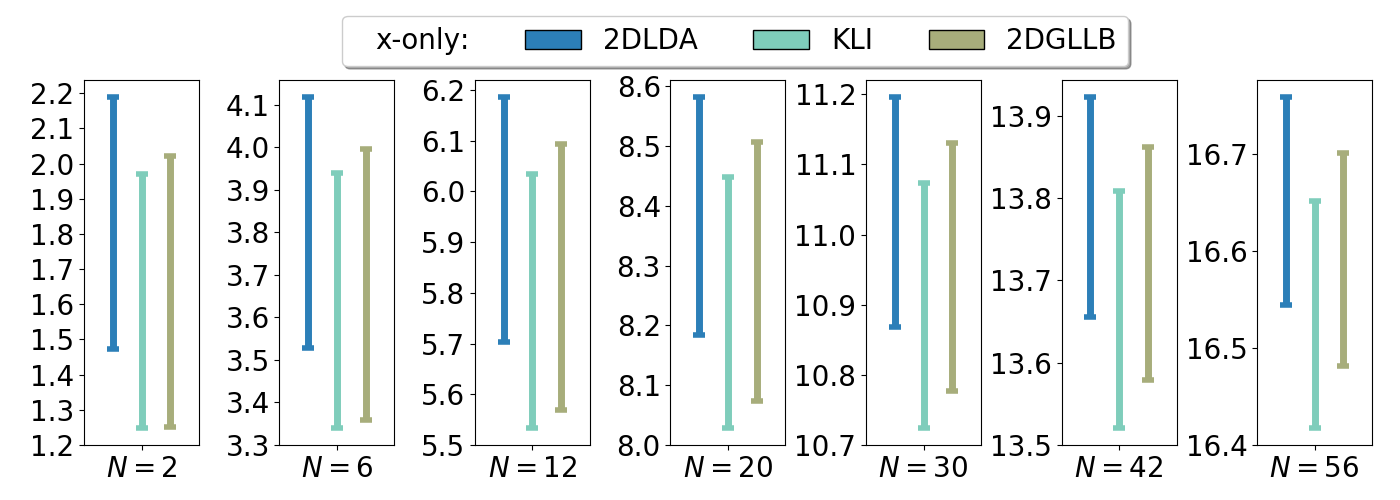
Figures 3 and 4 visualize all the aforementioned quantities for QDs with varying and , respectively, computed at the level of various exchange-only (x-only) approximations. Using, again, the KLI results as a reference, we note that the 2DLDA overestimates both the ionization potential and electron affinity for all the QDs. This is due to the inaccurate KS eigenvalues and resulting from the erroneous long-range behavior of the 2DLDA x-potential. We also note that the 2DLDA tends to underestimate the fundamental gaps, even though the errors in and are at least partly canceled out in . In 2DGLLB instead the ionization potentials and electron affinities are improved individually. This can be ascribed to the improved description of Slater potential (especially of its tail) obtained via the 2DB88 approximation. The 2DGLLB slightly overestimates (underestimates) the fundamental gaps at lower (at higher ). Overall, the accuracy of the 2DGLLB for the fundamental gaps is comparable to that of the 2DLDA.
In detail, the mean absolute error for the ionization potentials is () in the 2DGLLB (2DLDA) case. For the electron affinities the error is () in the 2DGLLB (2DLDA) case. Finally, for the the fundamental gaps the error is () in the 2DGLLB (2DLDA) case. Furthermore – in line with the expectation that the 2DGLLB-SC potential is less adapted than the 2DGLLB potential to deal with finite systems – the 2DGLLB-SC mean absolute errors are , , and , respectively. We will consider the 2DGLLB-SC case more in detail for 2D periodic systems in the next section.

Finally, we examine cases for quantum dots including correlations. Here we consider a set of parabolic QDs () with and for which numerically exact configuration interaction results are available [90]. Our results are shown in Fig. 5. Overall, both 2DGLLB and 2DLDA yield accurate results in all considered cases. In particular, the 2DGLLB slightly underestimates the gap for all cases, while the 2DLDA underestimates the gap for closed-shell systems () and overestimates the gap in the open-shell systems (). Both and are systematically more accurate in 2DGLLB than in 2DLDA. The mean absolute error for the fundamental gaps is and for the 2DGLLB and 2DLDA case, respectively.
III.2 Periodic systems: Artificial graphene
III.2.1 Model and parameters

To test the proposed approached in periodic 2D systems, we consider artificial graphene [2, 3, 4, 5, 6, 7, 8, 9, 91], (AG) and its Kekulé distortion leading to a band-gap opening [6, 7]. In particular, we focus on AG realized in nanopatterned 2D electron gas in GaAs heterostructures [2, 3, 4, 5, 91] that can be modeled in real space with a hegagonal array of QDs [5, 92]. This system shows Dirac cones similar to conventional graphene, and the band structure can be tuned at will through, e.g., Kekulé distortion.
In Fig. 6, we show a schematic figure of the AG (left) and its Kekulé distortion, together with the rectangular unit cells for both cases. The calculations were performed in a non-primitive cell due to numerical restrictions, and thus the bands had to be unfolded as described in Refs. 5 and 92. The lattice constant is set to nm, and the QDs are modeled by a cylindrical hard-wall potential with radius nm. The grid spacing is set to nm. The potential depth of each QD is meV, and in the Kekulé case two of the four QDs in the unit cell are lowered by up to meV. We use the same GaAs parameters as in the previous section ( and ). We set four electrons in a unit cell, so that each QD is occupied by one electron. Such a low-density system is experimentally viable [93, 94, 95].
The irreducible Brillouin zone is sampled with a regular grid according to a modified Monkhorst-Pack scheme [96]. In order to compute the band structure, we sample equally spaced points along the path ---. Here, we will show energies in meV and lengths in nm in accordance with the previous works [3, 5, 92].
III.2.2 Results


In the upper panel of Fig. 7, we show the energy bands of the AG computed with 2DLDA, 2DGLLB-SC, and 2DGLLB, respectively. As expected, all the cases show Dirac cones with linear dispersion relation at the point. Since AG is a periodic system, . Because AG is a semimetal (with zero band gap), the top of the valence band and the bottom of the conduction band have the same energy, i.e., . Thus, also . The 2DGLLB(-SC) results show slightly smaller band dispersion than the 2DLDA counterpart.
In the lower panel of Fig. 7, we show the energy bands of AG with Kekulé distortion ( meV). As expected, the Kekulé distortion opens a gap at the point. The valence bands are qualitatively similar in 2DGLLB(-SC) and 2DLDA. However, as in the case of regular AG, the 2DGLLB(-SC) bands are less dispersive than in the LDA case. The conduction bands shows more differences. In particular, , while . This fact significantly affects the position of the conduction bands with respect to the bare KS bands.
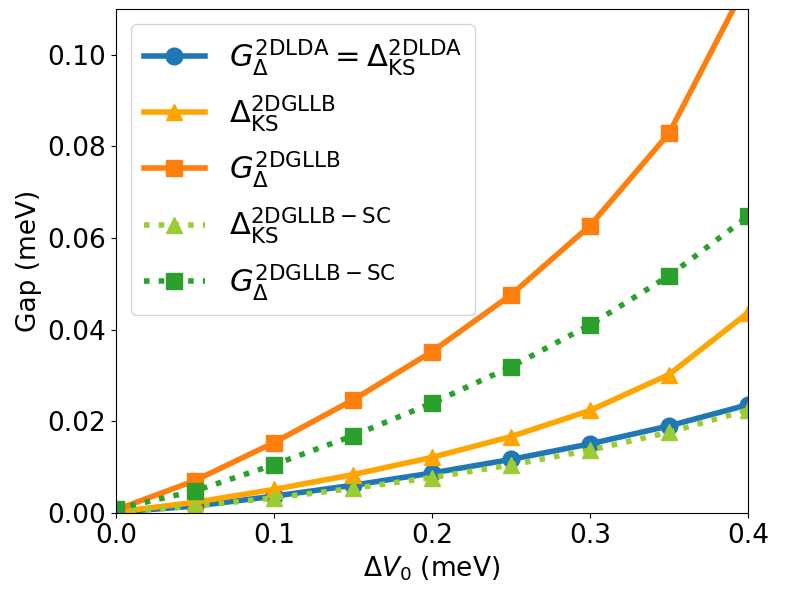
In order to examine the difference mentioned above, in Fig. 8 we plot the fundamental gaps and as a function of the distortion parameter . The differences clearly reflect the fact that for all periodic systems as . Instead, in the case of the 2DGLLB(-SC) potential, . For vanishing distortion, we recover the Dirac cones, i.e., . Fig. 8 also shows that the KS gaps are almost identical in the 2DLDA and 2DGLLB-SC cases. Both, however, differ from the case of the 2DGLLB-model potential.
According to Sec. II.1, we expect that the GLLB-SC results – possibly by including proper gradient corrections which were neglected here – should be closer to exact or close-to-exact benchmark results that could be obtained through, e.g., Hartree-Fock, GW, or equation-of-motion coupled cluster for 2D periodic systems. However, to the best of our knowledge, such benchmark results are not yet available.
IV Conclusions
In the past decades, advances in semiconductor technology have led to the development of artificial electronic systems in reduced dimensions. In the physics of two-dimensional (2D) electronic systems we have also witnessed a shift in the focus from single quantum dots to periodic arrays of various lattice configurations; thus following the rapid development of atomic two-dimensional materials.
However, the toolbox of electronic structure calculations for low-dimensional systems still requires vigorous efforts to reach the level that is currently available for regular atoms, molecules and solids in three dimensions. In this work, we have advanced a density functional approach via direct orbital-dependent modeling of Kohn-Sham potential. The modeling presented here is analogous to what has been successfully put forward for regular three-dimensional (3D) materials [62, 65, 71]. In particular, here we have worked out a shift from the domain of 3D atomic materials to the domain of 2D semiconductor devices.
Remarkably, the approach involves a computational cost which is comparable to that of a standard semi-local density functional for total energy calculations. Yet, it allows us to capture the fundamental gaps of single 2D quantum dots as well as of periodic array thereof by including key contributions which are beyond the bare Kohn-Sham gaps.
Further testing should be carried out to fully asses the quantitative aspects of the approach for 2D periodic systems. This will require non-trivial numerical work to implement accurate ab initio methodologies (such as a 2D version of the GW approach or equation-of-motion coupled cluster) that — to the best of our knowledge — are not readily available for the systems considered in this work. In any event, the proposed model potentials are extendable to meet higher demands in accuracy. These aspects will be examined in future works.
Acknowledgements.
S. P. acknowledges financial support through MIUR PRIN Grant No. 2017RKWTMY. C. A. R. acknowledges financial support from MIUR PRIN Grant 201795SBA3.References
- Martin [2020] R. M. Martin, Electronic Structure (Cambridge University Press, 2020), URL https://doi.org/10.1017/9781108555586.
- Park and Louie [2009] C.-H. Park and S. G. Louie, Nano Lett. 9, 1793 (2009).
- Gibertini et al. [2009] M. Gibertini, A. Singha, V. Pellegrini, M. Polini, G. Vignale, A. Pinczuk, L. N. Pfeiffer, and K. W. West, Phys. Rev. B 79, 241406 (2009), URL https://link.aps.org/doi/10.1103/PhysRevB.79.241406.
- Singha et al. [2011] A. Singha, M. Gibertini, B. Karmakar, S. Yuan, M. Polini, G. Vignale, M. I. Katsnelson, A. Pinczuk, L. N. Pfeiffer, K. W. West, et al., Science 332, 1176 (2011), ISSN 0036-8075, eprint https://science.sciencemag.org/content/332/6034/1176.full.pdf, URL https://science.sciencemag.org/content/332/6034/1176.
- Räsänen et al. [2012] E. Räsänen, C. A. Rozzi, S. Pittalis, and G. Vignale, Phys. Rev. Lett. 108, 2 (2012), ISSN 00319007, eprint 1201.1734.
- Gomes et al. [2012] K. K. Gomes, W. Mar, W. Ko, F. Guinea, and H. C. Manoharan, Nature 483, 306 (2012).
- Paavilainen et al. [2016] S. Paavilainen, M. Ropo, J. Nieminen, J. Akola, and E. Räsänen, Nano Lett. 16, 3519 (2016).
- Tarruell et al. [2012] L. Tarruell, D. Greif, T. Uehlinger, G. Jotzu, and T. Esslinger, Nature 483, 302 (2012).
- Polini et al. [2013] M. Polini, F. Guinea, M. Lewenstein, H. C. Manoharan, and V. Pellegrini, Nat. Nanotechnol. 8, 625 (2013).
- Slot et al. [2017] M. R. Slot, T. S. Gardenier, P. H. Jacobse, G. C. P. van Miert, S. N. Kempkes, S. J. M. Zevenhuizen, C. M. Smith, D. Vanmaekelbergh, and I. Swart, Nature Physics 13, 672 (2017), URL https://doi.org/10.1038/nphys4105.
- Khajetoorians et al. [2019] A. A. Khajetoorians, D. Wegner, A. F. Otte, and I. Swart, Nature Reviews Physics 1, 703 (2019), URL https://doi.org/10.1038/s42254-019-0108-5.
- Bistritzer and MacDonald [2011] R. Bistritzer and A. H. MacDonald, Proceedings of the National Academy of Sciences 108, 12233 (2011), URL https://doi.org/10.1073/pnas.1108174108.
- Cao et al. [2018a] Y. Cao, V. Fatemi, S. Fang, K. Watanabe, T. Taniguchi, E. Kaxiras, and P. Jarillo-Herrero, Nature 556, 43 (2018a).
- Cao et al. [2018b] Y. Cao, V. Fatemi, A. Demir, S. Fang, S. L. Tomarken, J. Y. Luo, J. D. Sanchez-Yamagishi, K. Watanabe, T. Taniguchi, E. Kaxiras, et al., Nature 556, 80 (2018b), URL https://doi.org/10.1038/nature26154.
- Kim et al. [2017] K. Kim, A. DaSilva, S. Huang, B. Fallahazad, S. Larentis, T. Taniguchi, K. Watanabe, B. J. LeRoy, A. H. MacDonald, and E. Tutuc, Proceedings of the National Academy of Sciences 114, 3364 (2017), URL https://doi.org/10.1073/pnas.1620140114.
- Chen et al. [2019] P.-Y. Chen, X.-Q. Zhang, Y.-Y. Lai, E.-C. Lin, C.-A. Chen, S.-Y. Guan, J.-J. Chen, Z.-H. Yang, Y.-W. Tseng, S. Gwo, et al., Advanced Materials 31, 1901077 (2019), URL https://doi.org/10.1002/adma.201901077.
- Tartakovskii [2019] A. Tartakovskii, Nature Reviews Physics 2, 8 (2019), URL https://doi.org/10.1038/s42254-019-0136-1.
- Yankowitz et al. [2019] M. Yankowitz, S. Chen, H. Polshyn, Y. Zhang, K. Watanabe, T. Taniguchi, D. Graf, A. F. Young, and C. R. Dean, Science 363, 1059 (2019), URL https://doi.org/10.1126/science.aav1910.
- Lu et al. [2019] X. Lu, P. Stepanov, W. Yang, M. Xie, M. A. Aamir, I. Das, C. Urgell, K. Watanabe, T. Taniguchi, G. Zhang, et al., Nature 574, 653 (2019), URL https://doi.org/10.1038/s41586-019-1695-0.
- Stepanov et al. [2020] P. Stepanov, I. Das, X. Lu, A. Fahimniya, K. Watanabe, T. Taniguchi, F. H. L. Koppens, J. Lischner, L. Levitov, and D. K. Efetov, Nature 583, 375 (2020), URL https://doi.org/10.1038/s41586-020-2459-6.
- Reserbat-Plantey et al. [2021] A. Reserbat-Plantey, I. Epstein, I. Torre, A. T. Costa, P. A. D. Gonçalves, N. A. Mortensen, M. Polini, J. C. W. Song, N. M. R. Peres, and F. H. L. Koppens, ACS Photonics 8, 85 (2021), URL https://doi.org/10.1021/acsphotonics.0c01224.
- [22] In this work, we use the term “2D system” to denote a system which is obtained via quantum confinement in one spatial direction. The paradigmatic case is the one of the well-known 2D homogeneous electron gas [Giuliani2005]. Thus graphene — which is formed by a 2D layer of actual three-dimensional atoms — is in our terminology a 2D material rather than a 2D system. Instead, the artificial graphene considered within our applications is a 2D system.
- Perdew and Kurth [2003] J. P. Perdew and S. Kurth, Density Functionals for Non-relativistic Coulomb Systems in the New Century. (Springer, Berlin, Heidelberg, 2003), In: Fiolhais C., Nogueira F., Marques M.A.L. (eds) A Primer in Density Functional Theory. Lecture Notes in Physics, vol 620. .
- Scuseria and Staroverov [2005] G. E. Scuseria and V. N. Staroverov, in Theory and Applications of Computational Chemistry, edited by C. E. Dykstra, G. Frenking, K. S. Kim, and G. E. Scuseria (Elsevier, Amsterdam, 2005), pp. 669 – 724, ISBN 978-0-444-51719-7, URL http://www.sciencedirect.com/science/article/pii/B9780444517197500676.
- Mardirossian and Head-Gordon [2017] N. Mardirossian and M. Head-Gordon, Molecular Physics 115, 2315 (2017), eprint https://doi.org/10.1080/00268976.2017.1333644, URL https://doi.org/10.1080/00268976.2017.1333644.
- Attaccalite et al. [2002] C. Attaccalite, S. Moroni, P. Gori-Giorgi, and G. B. Bachelet, Phys. Rev. Lett. 88, 256601 (2002), URL https://link.aps.org/doi/10.1103/PhysRevLett.88.256601.
- Pittalis et al. [2007] S. Pittalis, E. Räsänen, N. Helbig, and E. K. U. Gross, Phys. Rev. B 76, 235314 (2007), URL https://link.aps.org/doi/10.1103/PhysRevB.76.235314.
- Pittalis et al. [2008] S. Pittalis, E. Räsänen, and M. A. L. Marques, Phys. Rev. B 78, 195322 (2008).
- Pittalis et al. [2009a] S. Pittalis, E. Räsänen, J. G. Vilhena, and M. A. L. Marques, Phys. Rev. A 79, 12503 (2009a), ISSN 1050-2947, URL http://link.aps.org/doi/10.1103/PhysRevA.79.012503.
- Räsänen et al. [2009] E. Räsänen, S. Pittalis, C. R. Proetto, and E. K. U. Gross, Phys. Rev. B 79, 121305 (2009), URL https://link.aps.org/doi/10.1103/PhysRevB.79.121305.
- Pittalis et al. [2009b] S. Pittalis, E. Räsänen, C. R. Proetto, and E. K. U. Gross, Phys. Rev. B 79, 085316 (2009b), URL https://link.aps.org/doi/10.1103/PhysRevB.79.085316.
- Pittalis et al. [2009c] S. Pittalis, E. Räsänen, and E. K. U. Gross, Phys. Rev. A 80, 032515 (2009c), URL https://link.aps.org/doi/10.1103/PhysRevA.80.032515.
- Pittalis and Räsänen [2009] S. Pittalis and E. Räsänen, Phys. Rev. B 80, 165112 (2009), URL https://link.aps.org/doi/10.1103/PhysRevB.80.165112.
- Räsänen and Pittalis [2010] E. Räsänen and S. Pittalis, Physica E: Low-dimensional Systems and Nanostructures 42, 1232 (2010), ISSN 1386-9477, 18th International Conference on Electron Properties of Two-Dimensional Systems, URL https://www.sciencedirect.com/science/article/pii/S1386947709005645.
- Pittalis and Räsänen [2010a] S. Pittalis and E. Räsänen, Phys. Rev. B 82, 165123 (2010a), URL https://link.aps.org/doi/10.1103/PhysRevB.82.165123.
- Räsänen et al. [2010] E. Räsänen, S. Pittalis, and C. R. Proetto, Phys. Rev. B 81, 195103 (2010), URL https://link.aps.org/doi/10.1103/PhysRevB.81.195103.
- Pittalis and Räsänen [2010b] S. Pittalis and E. Räsänen, Phys. Rev. B 82, 195124 (2010b), URL https://link.aps.org/doi/10.1103/PhysRevB.82.195124.
- Pittalis et al. [2010] S. Pittalis, E. Räsänen, and C. R. Proetto, Phys. Rev. B 81, 115108 (2010), URL https://link.aps.org/doi/10.1103/PhysRevB.81.115108.
- Vilhena et al. [2014] J. G. Vilhena, E. Räsänen, M. A. L. Marques, and S. Pittalis, Journal of Chemical Theory and Computation 10, 1837 (2014), pMID: 26580514, eprint https://doi.org/10.1021/ct4010728, URL https://doi.org/10.1021/ct4010728.
- Jana and Samal [2017] S. Jana and P. Samal, The Journal of Physical Chemistry A 121, 4804 (2017), pMID: 28581752, eprint https://doi.org/10.1021/acs.jpca.7b03686, URL https://doi.org/10.1021/acs.jpca.7b03686.
- Patra et al. [2018a] A. Patra, S. Jana, and P. Samal, The Journal of Physical Chemistry A 122, 3455 (2018a), pMID: 29561615, eprint https://doi.org/10.1021/acs.jpca.8b00429, URL https://doi.org/10.1021/acs.jpca.8b00429.
- Patra et al. [2018b] A. Patra, S. Jana, and P. Samal, J. Chem. Phys. 148, 134117 (2018b), eprint https://doi.org/10.1063/1.5019251, URL https://doi.org/10.1063/1.5019251.
- Jana et al. [2018] S. Jana, A. Patra, and P. Samal, Physica E 97, 268 (2018), ISSN 1386-9477, URL http://www.sciencedirect.com/science/article/pii/S1386947717314753.
- Patra and Samal [2019] A. Patra and P. Samal, Chem. Phys. Lett. 720, 70 (2019), ISSN 0009-2614, URL http://www.sciencedirect.com/science/article/pii/S0009261419301058.
- Godby et al. [1988] R. W. Godby, M. Schlüter, and L. J. Sham, Phys. Rev. B 37, 10159 (1988), URL https://link.aps.org/doi/10.1103/PhysRevB.37.10159.
- Aryasetiawan and Gunnarsson [1998] F. Aryasetiawan and O. Gunnarsson, Rep. Prog. Phys. 61, 237 (1998), URL http://stacks.iop.org/0034-4885/61/i=3/a=002.
- Onida et al. [2002] G. Onida, L. Reining, and A. Rubio, Rev. Mod. Phys. 74, 601 (2002), URL https://link.aps.org/doi/10.1103/RevModPhys.74.601.
- Grüning et al. [2006] M. Grüning, A. Marini, and A. Rubio, J. Chem. Phys. 124, 154108 (2006).
- Heyd et al. [2003] J. Heyd, G. E. Scuseria, and M. Ernzerhof, J. Chem. Phys. 118, 8207 (2003).
- Heyd et al. [2006] J. Heyd, G. E. Scuseria, and M. Ernzerhof, J. Chem. Phys. 124, 219906 (2006).
- Stein et al. [2010] T. Stein, H. Eisenberg, L. Kronik, and R. Baer, Phys. Rev. Lett. 105, 266802 (2010), URL https://link.aps.org/doi/10.1103/PhysRevLett.105.266802.
- Kronik et al. [2012] L. Kronik, T. Stein, S. Refaely-Abramson, and R. Baer, J. Chem. Theory Comput. 8, 1515 (2012).
- Franchini [2014] C. Franchini, J. Phys. Condens. Matter 26, 253202 (2014), URL http://stacks.iop.org/0953-8984/26/i=25/a=253202.
- Perdew et al. [2017] J. P. Perdew, W. Yang, K. Burke, Z. Yang, E. K. U. Gross, M. Scheffler, G. E. Scuseria, T. M. Henderson, I. Y. Zhang, A. Ruzsinszky, et al., PNAS 114, 2801 (2017), ISSN 0027-8424.
- Kraisler and Kronik [2013] E. Kraisler and L. Kronik, Phys. Rev. Lett. 110, 126403 (2013), URL https://link.aps.org/doi/10.1103/PhysRevLett.110.126403.
- Kraisler and Kronik [2014] E. Kraisler and L. Kronik, J. Chem. Phys. 140, 18A540 (2014), URL https://doi.org/10.1063/1.4871462.
- Görling [2015] A. Görling, Phys. Rev. B 91, 245120 (2015), URL https://link.aps.org/doi/10.1103/PhysRevB.91.245120.
- Gritsenko et al. [2016] O. V. Gritsenko, Ł. M. Mentel, and E. J. Baerends, The J. Chem. Phys. 144, 204114 (2016).
- Senjean and Fromager [2018] B. Senjean and E. Fromager, Phys. Rev. A 98, 022513 (2018), URL https://link.aps.org/doi/10.1103/PhysRevA.98.022513.
- Senjean and Fromager [2020] B. Senjean and E. Fromager, International Journal of Quantum Chemistry 120, e26190 (2020), eprint https://onlinelibrary.wiley.com/doi/pdf/10.1002/qua.26190, URL https://onlinelibrary.wiley.com/doi/abs/10.1002/qua.26190.
- Hodgson et al. [2021] M. J. P. Hodgson, J. Wetherell, and E. Fromager, Phys. Rev. A 103, 012806 (2021), URL https://link.aps.org/doi/10.1103/PhysRevA.103.012806.
- Gritsenko et al. [1995] O. Gritsenko, R. van Leeuwen, E. Van Lenthe, and E. J. Baerends, Phys. Rev. A 51, 1944 (1995), ISSN 10502947.
- Tran and Blaha [2009] F. Tran and P. Blaha, Phys. Rev. Lett. 102, 226401 (2009), URL https://link.aps.org/doi/10.1103/PhysRevLett.102.226401.
- Kuisma et al. [2010a] M. Kuisma, J. Ojanen, J. Enkovaara, and T. T. Rantala, Phys. Rev. B 82, 115106 (2010a), URL https://link.aps.org/doi/10.1103/PhysRevB.82.115106.
- Kuisma et al. [2010b] M. Kuisma, J. Ojanen, J. Enkovaara, and T. T. Rantala, Phys. Rev. B 82, 1 (2010b), ISSN 10980121, eprint 1003.0296.
- Jiang [2013] H. Jiang, J. Chem. Phys. 138, 134115 (2013).
- Armiento and Kümmel [2013] R. Armiento and S. Kümmel, Phys. Rev. Lett. 111, 036402 (2013), URL https://link.aps.org/doi/10.1103/PhysRevLett.111.036402.
- Cerqueira et al. [2014] T. F. T. Cerqueira, M. J. T. Oliveira, and M. A. L. Marques, J. Chem. Theory Comput. 10, 5625 (2014).
- Castelli et al. [2012] I. E. Castelli, T. Olsen, S. Datta, D. D. Landis, S. Dahl, K. S. Thygesen, and K. W. Jacobsen, Energy Environ. Sci. 5, 5814 (2012), URL http://dx.doi.org/10.1039/C1EE02717D.
- Kohut et al. [2014] S. V. Kohut, I. G. Ryabinkin, and V. N. Staroverov, The Journal of Chemical Physics 140, 18A535 (2014), eprint https://doi.org/10.1063/1.4871500, URL https://doi.org/10.1063/1.4871500.
- Baerends [2017] E. J. Baerends, Phys. Chem. Chem. Phys. 19, 15639 (2017), URL http://dx.doi.org/10.1039/C7CP02123B.
- Tran et al. [2018] F. Tran, S. Ehsan, and P. Blaha, Phys. Rev. Materials 2, 023802 (2018), URL https://link.aps.org/doi/10.1103/PhysRevMaterials.2.023802.
- Borlido et al. [2019] P. Borlido, T. Aull, A. W. Huran, F. Tran, M. A. L. Marques, and S. Botti, Journal of Chemical Theory and Computation 15, 5069 (2019), pMID: 31306006, eprint https://doi.org/10.1021/acs.jctc.9b00322, URL https://doi.org/10.1021/acs.jctc.9b00322.
- Rauch et al. [2020] T. c. v. Rauch, M. A. L. Marques, and S. Botti, Phys. Rev. B 101, 245163 (2020), URL https://link.aps.org/doi/10.1103/PhysRevB.101.245163.
- Guandalini et al. [2019] A. Guandalini, C. A. Rozzi, E. Räsänen, and S. Pittalis, Phys. Rev. B 99, 125140 (2019), URL https://link.aps.org/doi/10.1103/PhysRevB.99.125140.
- Krieger et al. [1992] J. B. Krieger, Y. Li, and G. J. Iafrate, Phys. Rev. A 45, 101 (1992), ISSN 10502947.
- Kümmel and Kronik [2008] S. Kümmel and L. Kronik, Rev. Mod. Phys. 80, 3 (2008), URL https://link.aps.org/doi/10.1103/RevModPhys.80.3.
- Tran et al. [2016] F. Tran, P. Blaha, M. Betzinger, and S. Blügel, Phys. Rev. B 94, 165149 (2016), URL https://link.aps.org/doi/10.1103/PhysRevB.94.165149.
- Rajagopal and Kimball [1977] A. K. Rajagopal and J. C. Kimball, Phys. Rev. B 15, 2819 (1977), URL https://link.aps.org/doi/10.1103/PhysRevB.15.2819.
- Becke [1988] A. D. Becke, Physical Review A 38, 3098 (1988), URL https://doi.org/10.1103/physreva.38.3098.
- Perdew et al. [2008] J. P. Perdew, A. Ruzsinszky, G. I. Csonka, O. A. Vydrov, G. E. Scuseria, L. A. Constantin, X. Zhou, and K. Burke, Physical Review Letters 100 (2008), URL https://doi.org/10.1103/physrevlett.100.136406.
- Tanatar and Ceperley [1989] B. Tanatar and D. M. Ceperley, Phys. Rev. B 39, 5005 (1989), URL https://link.aps.org/doi/10.1103/PhysRevB.39.5005.
- Perdew et al. [1982] J. P. Perdew, R. G. Parr, M. Levy, and J. L. Balduz, Phys. Rev. Lett. 49, 1691 (1982), URL https://link.aps.org/doi/10.1103/PhysRevLett.49.1691.
- Perdew and Levy [1983] J. P. Perdew and M. Levy, Phys. Rev. Lett. 51, 1884 (1983), URL https://link.aps.org/doi/10.1103/PhysRevLett.51.1884.
- Sham and Schlüter [1985] L. J. Sham and M. Schlüter, Phys. Rev. B 32, 3883 (1985), URL https://link.aps.org/doi/10.1103/PhysRevB.32.3883.
- Andrade et al. [2015] X. Andrade, D. Strubbe, U. De Giovannini, A. H. Larsen, M. J. T. Oliveira, J. Alberdi-Rodriguez, A. Varas, I. Theophilou, N. Helbig, M. J. Verstraete, et al., Phys. Chem. Chem. Phys. 17, 31371 (2015), URL http://dx.doi.org/10.1039/C5CP00351B.
- Castro et al. [2006] A. Castro, H. Appel, M. Oliveira, C. A. Rozzi, X. Andrade, F. Lorenzen, M. A. L. Marques, E. K. U. Gross, and A. Rubio, Phys. status solidi B 243, 2465 (2006), URL https://onlinelibrary.wiley.com/doi/abs/10.1002/pssb.200642067.
- Marques et al. [2003] M. A. Marques, A. Castro, G. F. Bertsch, and A. Rubio, Comput. Phys. Commun. 151, 60 (2003), ISSN 0010-4655, URL http://www.sciencedirect.com/science/article/pii/S0010465502006860.
- Reimann and Manninen [2002] S. M. Reimann and M. Manninen, Rev. Mod. Phys. 74, 1283 (2002), URL https://link.aps.org/doi/10.1103/RevModPhys.74.1283.
- Capelle et al. [2007] K. Capelle, M. Borgh, K. Kärkkäinen, and S. M. Reimann, Phys. Rev. Lett. 99, 010402 (2007), URL https://link.aps.org/doi/10.1103/PhysRevLett.99.010402.
- Du et al. [2018] L. Du, S. Wang, D. Scarabelli, L. N. Pfeiffer, K. W. West, S. Fallahi, G. C. Gardner, M. J. Manfra, V. Pellegrini, S. J. Wind, et al., Nature Communications 9 (2018), URL https://doi.org/10.1038/s41467-018-05775-4.
- Kylänpä et al. [2016] I. Kylänpä, F. Berardi, E. Räsänen, P. Garcìa-Gonzàlez, C. A. Rozzi, and A. Rubio, New J. Phys. 18 (2016), ISSN 13672630.
- Hirjibehedin et al. [2002] C. F. Hirjibehedin, A. Pinczuk, B. S. Dennis, L. N. Pfeiffer, and K. W. West, Phys. Rev. B 65, 161309 (2002), URL https://link.aps.org/doi/10.1103/PhysRevB.65.161309.
- Hirjibehedin et al. [2005] C. F. Hirjibehedin, I. Dujovne, A. Pinczuk, B. S. Dennis, L. N. Pfeiffer, and K. W. West, Phys. Rev. Lett. 95, 066803 (2005), URL https://link.aps.org/doi/10.1103/PhysRevLett.95.066803.
- García et al. [2005] C. P. García, V. Pellegrini, A. Pinczuk, M. Rontani, G. Goldoni, E. Molinari, B. S. Dennis, L. N. Pfeiffer, and K. W. West, Phys. Rev. Lett. 95, 266806 (2005), URL https://link.aps.org/doi/10.1103/PhysRevLett.95.266806.
- Pack and Monkhorst [1977] J. D. Pack and H. J. Monkhorst, Phys. Rev. B 16, 1748 (1977), URL https://link.aps.org/doi/10.1103/PhysRevB.16.1748.