Deep Extended Feedback Codes

Abstract

A new deep-neural-network (DNN) based error correction encoder architecture for channels with feedback, called Deep Extended Feedback (DEF), is presented in this paper. The encoder in the DEF architecture transmits an information message followed by a sequence of parity symbols which are generated based on the message as well as the observations of the past forward channel outputs sent to the transmitter through a feedback channel. DEF codes generalize Deepcode [1] in several ways: parity symbols are generated based on forward-channel output observations over longer time intervals in order to provide better error correction capability; and high-order modulation formats are deployed in the encoder so as to achieve increased spectral efficiency. Performance evaluations show that DEF codes have better performance compared to other DNN-based codes for channels with feedback.

I Introduction

The fifth generation (5G) wireless cellular networks’ New Radio (NR) access technology has been recently specified by the $3^{\rm rd}$ Generation Partnership Project (3GPP). NR already fulfills demanding requirements of throughput, reliability and latency. However, new use cases stemming from new application domains (such as industrial automation, vehicular communications or medical applications) call for further significant enhancements. For instance, some typical Industrial Internet of Things (IIoT) applications would need considerably higher reliability and shorter transmission delay compared to what 5G/NR can provide nowadays.

Error correction coding is a key physical layer functionality for guaranteeing the required performance levels. In conventional systems, error correction is accomplished by linear binary codes such as polar codes [2], Low Density Parity Check (LDPC) codes [3] or turbo codes [4], possibly combined with retransmission mechanisms such as Hybrid Automatic Request (HARQ) [5]. HARQ performs an initial transmission followed by a variable number of subsequent incremental redundancy transmissions until the receiver notifies successful decoding to the transmitter. Short acknowledgment (ACK) or negative ACK (NACK) messages are sent through a feedback channel in order to inform the transmitter about decoding success. By usage of simple ACK/NACK feedback messages, conventional HARQ practically limits the gains that could potentially be obtained by an extensive and more efficient use of the feedback channel. Codes that make full use of feedback potentially achieve improved performance compared to conventional codes, as predicted in [6].

Finding good codes for channels with feedback is a notoriously difficult problem. Several coding methods for channels with feedback have been proposed – see for example [7, 8, 9, 10, 11]. However, all known solutions either do not approach the performance predicted in [6] or exhibit unaffordable complexity. Promising progress has been made recently by applying Machine Learning (ML) methods [1], where both encoder and decoder are implemented as two separate Deep Neural Networks (DNNs). The DNNs’ coefficients are determined through a joint encoder-decoder training procedure whereby encoder and decoder influence each other. In that sense, the chosen decoder structure has impact on the resulting code – a previously unseen feature. Known DNN-based feedback codes [1] use different recurrent neural network (NN) architectures – recurrent NNs (RNNs) and gated recurrent units (GRUs) are used in [1]; long-short term memory (LSTM) architectures have been mentioned in a preprint of [1] as a potential alternative to RNNs for the encoder.

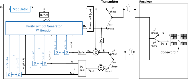
Figure 1: DEF encoder structure. Each “$D$” block represents a unit-time delay. Blue blocks and signals denote new functionalities compared to prior solutions.

A new DNN-based code for channels with feedback called Deep Extended Feedback (DEF) code is presented in this paper. The encoder transmits an information message followed by a sequence of parity symbols which are generated based on the message and on observations of the past forward channel outputs obtained through the feedback channel. Known DNN-based codes for channels with feedback [1] compute their parity symbols based on the information message and on the most recent information received through the feedback channel. The DEF code is based on feedback extension, which consists in extending the encoder input so as to comprise delayed versions of feedback signals. Thus, the DEF encoder input comprises the most recent feedback signal and a set of past feedback signals within a given time window. A similar approach could be used in the decoder to extend its input so as to comprise delayed versions of received signals in a given time window. However, it can be shown that such a generalization of the decoder does not bring any benefit and therefore it will not be considered in the definition of DEF codes. The extended-feedback encoder architecture is combined with different NN architectures of recurrent type – RNN, GRU and LSTM. The DEF code generalizes Deepcode [1] along several directions. Its major benefits can be summarized as follows:

• Improved error correction capability obtained by feedback extension. The DEF code generates parity symbols based on feedbacks in a longer time window, thereby introducing long-range dependencies between parity symbols. As the above long-range dependencies are a necessary ingredient of all good error correcting codes, it is expected that feedback extension will bring performance improvements;

• Higher spectral efficiency obtained by usage of QAM/PAM modulations. The DEF code uses quadrature amplitude modulation (QAM) with arbitrary order, thereby potentially achieving higher spectral efficiency;

In this work, we initially focus on DEF codes’ performance evaluation over channels with noiseless feedback, where the forward-channel output observations are sent uncorrupted to the encoder. We also provide preliminary performance evaluations of the DEF code with noisy feedback.

Notation: Lowercase and uppercase letters denote scalar (real or complex) values. For any pair of positive integers $a$ and $b$ with $a<b$, $[a:b]$ denotes the sequence of integers $[a,a+1,\ldots,b]$, sorted in increasing order. Boldface lowercase letters (e.g., $\mathbf{b}$) denote vectors; unless otherwise specified, all vectors are assumed to be column vectors. $b(i)$ denotes the $i^{\rm th}$ element of $\mathbf{b}$; $\mathbf{b}(j:k),j<k,$ denotes the sub-vector that contains the elements of $\mathbf{b}$ with indices in $[j:k]$. Boldface uppercase letters like $\mathbf{A}$ denote matrices; $a_{i,j}$ represents the element of $\mathbf{A}$ in the $i^{\rm th}$ row and $j^{\rm th}$ column. Notation $f(\mathbf{v})$, where $f$ is a function taking a scalar input, indicates the vector obtained by applying $f$ to each element of $\mathbf{v}$. Hadamard (i.e., element-wise) product is denoted by $\circ$.

II Definition of Deep Extended Feedback Code

The Deep Extended Feedback (DEF) code is the set of codewords produced by the DEF encoder shown in Fig. 1. Blue blocks and signals in Fig. 1 denote the new functionalities of the DEF code compared to Deepcode [1] – extended feedback is shown by the unit-time delay blocks labeled “$D$” and their corresponding input/ouput signals; QAM/PAM symbols are produced by the block labeled “Modulator”. DEF code and Deepcode operate according to the same encoding procedure as described afterwards. The novel DEF code features will be treated in dedicated subsections.

The encoding procedure consists of two phases. In the first phase, an $L$-bit information message $\mathbf{m}=(m(0),\ldots,m(L-1))$ is mapped to a sequence of real symbols $\mathbf{x}=(x(0),\ldots,x(K-1))$, hereafter called systematic symbols.

The modulation sequence $\mathbf{x}$ is transmitted on the forward channel. The corresponding sequence $\mathbf{\bar{x}}$ observed by the receiver is given by

$$\mathbf{\bar{x}}=\mathbf{x}+\mathbf{n}_{0}$$ (1)

where $\mathbf{n}_{0}$ represents additive white Gaussian noise (AWGN) and other possible forward-channel impairments. In the performance evaluations of Section IV, $\mathbf{n}_{0}$ is modeled as a sequence of white Gaussian noise samples. The receiver stores the observed signal $\mathbf{\bar{x}}$ locally and immediately echoes it back to the transmitter through the feedback channel. A corresponding sequence

$$\mathbf{\tilde{x}}=\mathbf{\bar{x}}+\mathbf{g}_{0}$$ (2)

is obtained at the transmitter, where $\mathbf{g}_{0}$ represents additive white Gaussian noise and other possible feedback-channel impairments.

In the second phase, for each element $x(k)$ of $\mathbf{x}$, the encoder computes a corresponding sequence of parity symbols

$$\mathbf{p}_{k}=(p_{k}(0),\ldots,p_{k}(P-1)),\quad k=0,\ldots,K-1$$ (3)

and transmits it through the forward channel. $P$ is the number of parity symbols that the encoder generates per systematic symbol. Thus, the total number of transmitted symbols is $K(1+P)$. The DEF code rate is defined as the ratio of the message length $L$ over $K(1+P)$, that is:

$$R_{\rm DEF}\triangleq\frac{L}{K(1+P)}.$$ (4)

The receiver observes a set of corresponding parity symbols sequences $\bar{\mathbf{p}}_{k},k=0,\ldots,K-1$. $\bar{\mathbf{p}}_{k}$ can be written as follows:

$$\bar{\mathbf{p}}_{k}=\mathbf{p}_{k}+\mathbf{v}_{k},$$ (5)

where $\mathbf{v}_{k}=(v_{k}(0),\ldots,v_{k}(P-1))$ represents additive white Gaussian noise and other forward channel impairments. $\bar{\mathbf{p}}_{k}$ is immediately echoed back to the transmitter through the feedback channel so as to obtain

$$\mathbf{\tilde{p}}_{k}=\mathbf{\bar{p}}_{k}+\mathbf{g}_{k},$$ (6)

where $\mathbf{g}_{k}$ represents additive white Gaussian noise and other feedback channel impairments.

The DEF codeword is defined as $\mathbf{z}=(z(0),\ldots,z({(P+1)K-1}))$. The $j^{\rm th}$ codeword symbol is defined as follows:

$$z(j)\! \!=\! \!\left\{\begin{array}[]{ll}w(0)a(j)x(j),&0\leq j\leq K-1\\ w(l+1)a(k)p_{k}(l),&K\!\leq\!j\!\leq(P+1)K-1\end{array}\right.$$ (9)

$$l\! \!=\! \!(j-K)\;{\rm mod}\;P,$$

$$k\! \!=\! \!\left\lfloor(j-K)/P\right\rfloor,$$

where $w(0)$ and $w(l+1),l=0,\ldots,P-1,$ are codeword power levels, $a(k),k=0,\ldots,K-1,$ are symbol power levels, $x(j)$ is the $j^{\rm th}$ systematic symbol, and $p_{k}(l)$ is the $l^{\rm th}$ symbol of the $k^{\rm th}$ parity sequence (3). Codeword power levels reallocate the power among codeword symbols as follows: the systematic symbols are scaled by $w(0)$; the $1^{\rm st}$ parity symbol of each parity sequence is scaled by $w(1)$, the $2^{\rm nd}$ parity symbol of each parity sequence is scaled by $w(2)$, etc. Symbol power levels reallocate the power among codeword symbols as follows: $a(0)$ scales the amplitude of the $1^{\rm st}$ systematic symbol $x(0)$ and of the symbols of the $1^{\rm st}$ parity symbol sequence $\mathbf{p}_{0}$, $a(1)$ scales the amplitude of the $2^{\rm nd}$ systematic symbol $x(1)$ and of the symbols of the $2^{\rm nd}$ parity symbol sequence $\mathbf{p}_{1}$, $\ldots$ $a(K-1)$ scales the amplitude of the $K^{\rm th}$ systematic symbol $x(K-1)$ and of the symbols of the $K^{\rm th}$ parity symbol sequence $\mathbf{p}_{K-1}$. Power levels $w(l)$ and $a(k)$ are obtained by NN training. The following constraints preserve the codeword’s average power:

$$\sum_{l=0}^{P}w^{2}(l)=1,\;\;\sum_{k=0}^{K-1}a^{2}(k)=1.$$ (10)

II-A QAM/PAM Modulator

The DEF code modulator maps the $L$-bit information message $\mathbf{m}=(m(0),\ldots,m(L-1))$ to a sequence of real symbols $\mathbf{x}=(x(0),\ldots,x(K-1))$, hereafter called systematic symbols. Each pair of consecutive symbols $(x(2i),x(2i+1)),i=0,\ldots,K/2-1$, forms a complex QAM symbol $q(i)=x(2i)+x(2i+1)\sqrt{-1}$, where $q(i)$ is obtained by mapping $Q$ consecutive bits of $\mathbf{m}$ to $2^{Q}$-QAM. The above mapping produces $K=2L/Q$ real systematic symbols at the modulator output.

Examples of QAM/PAM mapping of order $Q=2$ and $Q=4$ are shown in Tab. I and Tab. II.

$m(2i),m(2i+1)$	$x(2i)$	$x(2i+1)$
$0,0$	1	1
$0,1$	1	-1
$1,0$	-1	1
$1,1$	-1	-1

TABLE I: Example of QAM/PAM mapping of order $Q=2$.

$m(4i),m(4i+1),m(4i+2),m(4i+3)$	$x(2i)$	$x(2i+1)$
$0,0,0,0$	3	3
$0,0,0,1$	3	1
$0,0,1,0$	3	-3
$0,0,1,1$	3	-1
$0,1,0,0$	1	3
$0,1,0,1$	1	1
$0,1,1,0$	-1	-3
$0,1,1,1$	-1	-1
$1,0,0,0$	-3	3
$1,0,0,1$	-3	1
$1,0,1,0$	-3	-3
$1,0,1,1$	-3	-1
$1,1,0,0$	-1	3
$1,1,0,1$	-1	1
$1,1,1,0$	-1	-3
$1,1,1,1$	-1	-1

TABLE II: Example of QAM/PAM mapping of order $Q=4$.

II-B Extended Feedback

We call Parity Symbol Generator (PSG) the encoder block that computes the parity symbol sequences (see Figure 1). Extended feedback consists of sending to the PSG a sequence of forward-channel output observations over longer time intervals compared to Deepcode [1]. The PSG input column vector at the $k^{\rm th}$ iteration is defined as follows:

$${\mathbf{i}}_{k}=\left[\begin{array}[]{c}x(k)\\ \mathbf{n}_{0}(k-\delta_{0}:k)\\ \mathbf{r}_{0}(k-\delta_{1}:k-1)\\ \ldots\\ \mathbf{r}_{P-1}(k-\delta_{P}:k-1)\\ \end{array}\right],$$ (11)

where $x(k)$ is the $k^{\rm th}$ systematic symbol, $\mathbf{n}_{0}(k-\delta_{0}:k)$ is a column vector of length $\delta_{0}+1$ which contains noise samples from the sequence $\mathbf{n}_{0}$ of (1), $\mathbf{r}_{l}(k-\delta_{l}:k-1)$ $(l=0,\ldots,P-1)$ is a column vector of length $\delta_{l}$ which contains noise samples from the sequence $\mathbf{r}_{l}$ of forward-channel noise samples that corrupt the $l^{\rm th}$ symbol of each parity symbol sequence, that is:

$$\mathbf{r}_{l}\triangleq(v_{0}(l),\ldots,v_{K-1}(l)),$$ (12)

where $v_{k}(l)$ $(k=0,\ldots,K-1)$ is the $l^{\rm th}$ sample of $\mathbf{v}_{k}$ in (5) and $\delta_{0},\ldots,\delta_{P}$ are arbitrary positive integers ($\delta_{0}$ can be 0), hereafter called the encoder input extensions. We note that the Deepcode [1] encoder can be recovered as a special case by setting $\delta_{0}=0$ and $\delta_{1}=\ldots=\delta_{P}=1$, which means that, in each iteration, only a single noise sample for each systematic or parity check symbol is used. The buffers in the DEF encoder contain the systematic symbol sequence $\mathbf{x}$ and the corresponding forward-noise sequence $\mathbf{n}_{0}$ of (1). Those sequences are generated during the first encoding phase and used by the PSG in the second phase.

II-C Parity Symbol Generator (PSG)

The core functionality of the DEF encoder is the computation of the parity check symbols, which is performed by the block denoted (PSG) (see Fig. 1). PSG computes the $k^{\rm th}$ parity symbol sequence $\mathbf{p}_{k}$ based on the $k^{\rm th}$ modulation symbol $x_{k}$ and a subset of the past forward-channel outputs.

Fig. 2 shows the structure of the PSG. In the $k^{\rm th}$ encoding iteration, the PSG generates a $k^{\rm th}$ parity symbol sequence $\mathbf{p}_{k}$ which consists of $P$ real parity symbols obtained as follows:

$$\mathbf{p}_{k}={\rm Norm}(e(\mathbf{h}_{k})),$$ (13)

where ${\bf{h}}_{k}$ – a real vector of arbitrary length $H_{0}$ – denotes the PSG state at time instant $k$, while function $e(\cdot)$ consists of a linear transformation applied to the PSG state $\mathbf{h}_{k}$ obtained as follows:

$$e(\mathbf{h}_{k})=\mathbf{A}\mathbf{h}_{k}+\mathbf{c},$$ (14)

where $\mathbf{A}$ has size ${P\times H_{0}}$ and $\mathbf{c}$ has length ${P}$. The above matrices $\mathbf{W}$, $\mathbf{Y}$, $\mathbf{A}$ and vectors $\mathbf{b}$, $\mathbf{c}$ are obtained by NN training. The ${\rm Norm}(\cdot)$ function normalizes the PSG output so that each parity symbol has zero mean and unit variance. The PSG state ${\bf{h}}_{k}$ is recursively computed as

$$\mathbf{h}_{k}=f(\mathbf{i}_{k},\mathbf{h}_{k-1}),$$ (15)

where function $f(\cdot)$ will be discussed below, and ${\bf i}_{k}$ is defined in (11). As for the initialization, we set $\mathbf{h}_{0}$ as the all-zero vector.

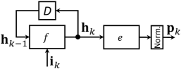
Figure 2: Structure of the PSG.

Functions $e$ and $f$ will be parameterized using DNNs. The structure of Fig. 2 corresponds to a recurrent architecture, and therefore, we will consider the following three recurrent architectures to model it: RNNs, GRUs and LSTMs.

II-C1 RNN

When modelled with an RNN, the function $f(\cdot)$ in (15) is defined as follows:

$$f(\mathbf{i}_{k},\mathbf{h}_{k-1})=\tanh(\mathbf{W}\mathbf{h}_{k-1}+\mathbf{Y}\mathbf{i}_{k}+\mathbf{b}),$$ (16)

where $\mathbf{W}$ is a state-transition matrix of size ${H_{0}\times H_{0}}$, $\mathbf{Y}$ is an input-state matrix of size ${H_{0}\times I}$ ($I$ is the length of vector $\mathbf{i}_{k}$), and $\mathbf{b}$ is a bias vector of length ${H_{0}}$. $\mathbf{W}$, $\mathbf{Y}$ and $\mathbf{b}$ are obtained by NN training.

II-C2 GRU

With a GRU, the function $f(\cdot)$ of (15) is defined as follows:

$$f(\mathbf{i}_{k},\mathbf{h}_{k-1}) = f_{0}(\mathbf{i}_{k},\mathbf{h}_{k-1})\circ(1-z(\mathbf{i}_{k},\mathbf{h}_{k-1}))$$ (17)

$$+ \mathbf{h}_{k-1}\circ z(\mathbf{i}_{k},\mathbf{h}_{k-1}).$$

The function $f_{0}(\cdot)$ in (17) is defined as follows:

$$f_{0}(\mathbf{i}_{k},\mathbf{h}_{k-1}) = \tanh((\mathbf{W}_{f}\mathbf{h}_{k-1}+\mathbf{b}_{h})\circ r(\mathbf{i}_{k},\mathbf{h}_{k-1})$$ (18)

$$+ \mathbf{Y}_{f}\mathbf{i}_{k}+\mathbf{b}_{i}).$$

The functions $z(\cdot)$ in (17) and $r(\cdot)$ in (18) are defined as follows:

$$z(\mathbf{i}_{k},\mathbf{h}_{k-1}) = \sigma(\mathbf{W}_{z}\mathbf{h}_{k-1}+\mathbf{Y}_{z}\mathbf{i}_{k}+\mathbf{b}_{z})$$ (19)

$$r(\mathbf{i}_{k},\mathbf{h}_{k-1}) = \sigma(\mathbf{W}_{r}\mathbf{h}_{k-1}+\mathbf{Y}_{r}\mathbf{i}_{k}+\mathbf{b}_{r})$$ (20)

where $\sigma(x)\triangleq(1+e^{-x})^{-1}$ denotes the sigmoid function. In eqns. (17)-(20), matrices $\mathbf{W}_{f},\mathbf{W}_{z},\mathbf{W}_{r},\mathbf{Y}_{f},\mathbf{Y}_{z},\mathbf{Y}_{r}$ and vectors $\mathbf{b}_{h},\mathbf{b}_{i},\mathbf{b}_{z},\mathbf{b}_{r}$ are obtained by NN training.

II-C3 LSTM

As for LSTM, the function $f(\cdot)$ of (15) is defined as follows:

$$f(\mathbf{i}_{k},\mathbf{h}_{k-1}) = f_{1}(\mathbf{i}_{k},\mathbf{h}_{k-1})\circ\tanh(\mathbf{s}_{k})$$ (21)

where $\mathbf{s}_{k}$ is the cell state at time instant $k$. The cell state provides long-term memory capability to the LSTM NN, whereas the state $\mathbf{h}_{k}$ provides short-term memory capability. The cell state is recursively computed as follows:

$$\mathbf{s}_{k} = f_{2}(\mathbf{i}_{k},\mathbf{h}_{k-1})\circ\mathbf{s}_{k-1}$$ (22)

$$+ f_{3}(\mathbf{i}_{k},\mathbf{h}_{k-1})\circ f_{4}(\mathbf{i}_{k},\mathbf{h}_{k-1}).$$

The function $f_{1}$ in (21) and functions $f_{2},f_{3}$ and $f_{4}$ in (22) are defined as follows:

$$f_{1}(\mathbf{i}_{k},\mathbf{h}_{k-1})\! \!=\! \!\sigma(\mathbf{W}_{1}\mathbf{h}_{k-1}+\mathbf{Y}_{1}\mathbf{i}_{k}+\mathbf{b}_{1})$$ (23)

$$f_{2}(\mathbf{i}_{k},\mathbf{h}_{k-1})\! \!=\! \!\sigma(\mathbf{W}_{2}\mathbf{h}_{k-1}+\mathbf{Y}_{2}\mathbf{i}_{k}+\mathbf{b}_{2})$$ (24)

$$f_{3}(\mathbf{i}_{k},\mathbf{h}_{k-1})\! \!=\! \!\sigma(\mathbf{W}_{3}\mathbf{h}_{k-1}+\mathbf{Y}_{3}\mathbf{i}_{k}+\mathbf{b}_{3})$$ (25)

$$f_{4}(\mathbf{i}_{k},\mathbf{h}_{k-1})\! \!=\! \!\tanh(\mathbf{W}_{4}\mathbf{h}_{k-1}+\mathbf{Y}_{4}\mathbf{i}_{k}+\mathbf{b}_{4})$$ (26)

In eqns. (23)-(26), matrices $\mathbf{W}_{1}$, $\mathbf{W}_{2}$, $\mathbf{W}_{3}$, $\mathbf{W}_{4}$, $\mathbf{Y}_{1}$, $\mathbf{Y}_{2}$, $\mathbf{Y}_{3}$, $\mathbf{Y}_{4}$ and vectors $\mathbf{b}_{1}$, $\mathbf{b}_{2}$, $\mathbf{b}_{3}$, $\mathbf{b}_{4}$ are obtained by NN training.

II-D Mitigation of Unequal Bit Error Distribution

It has been observed in [1] that the feedback codes based on RNNs exhibit a non-uniform bit error distribution, i.e., the final message bits typically have a significantly larger error rate compared to other bits. In order to mitigate the detrimental effect of non-uniform bit error distribution,  [1] introduced two countermeasures:

• Zero-padding. Zero-padding consists in appending at least one information bit with pre-defined value (e.g., zero) at the end of the message. The appended information bit(s) are discarded at the decoder, such that the positions affected by higher error rates carry no information.

• Power reallocation. Zero-padding alone is not enough to mitigate unequal errors, and moreover it reduces the effective code rate. Instead, power reallocation redistributes the power among the codeword symbols so as to provide better error protection to the message bits whose positions are more error-prone, i.e., the initial and final positions.

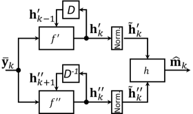
Figure 3: DEF decoder.

II-E DEF Decoder

In DNN-based codes, encoder and decoder are implemented as two separate DNNs whose coefficients are determined through a joint encoder-decoder training procedure. Therefore, the encoder structure has impact on the decoder coefficients obtained through training, and vice-versa. In that sense, the chosen decoder structure has impact on the resulting code.

The DEF decoder maps the received DEF codeword to a decoded message $\mathbf{\hat{m}}$ as follows:

$$\mathbf{\hat{m}}=g(\mathbf{\bar{x}},\mathbf{\bar{p}}^{(1)},\ldots,\mathbf{\bar{p}}^{(K)}).$$ (27)

The decoder consists of a bi-directional recurrent NN – GRU or LSTM – followed by a linear transformation and a sigmoid function. The bi-directional recurrent NN computes a sequence of forward-states $\mathbf{h}_{k}^{\prime}$ and backward-states $\mathbf{h}_{k}^{\prime\prime}$ as follows:

$$\mathbf{h}_{k}^{\prime} = f^{\prime}(\mathbf{\bar{y}}_{k},\mathbf{h}_{k-1}^{\prime})$$ (28)

$$\mathbf{h}_{k-1}^{\prime\prime} = f^{\prime\prime}(\mathbf{\bar{y}}_{k},\mathbf{h}_{k}^{\prime\prime})$$ (29)

where functions $f^{\prime},f^{\prime\prime}$ are defined as in (17) for the GRU-based decoder and as in (21) for the LSTM-based decoder, and the input column vector $\mathbf{\bar{y}}_{k}$ is defined as follows:

$$\mathbf{\bar{y}}_{k}=\left[\begin{array}[]{c}\mathbf{\bar{x}}(k-\gamma_{0}:k)\\ \mathbf{\bar{q}}_{0}(k-\gamma_{1}:k)\\ \ldots\\ \mathbf{\bar{q}}_{P-1}(k-\gamma_{P}:k)\end{array}\right],$$ (30)

where $\mathbf{\bar{x}}(k-\gamma_{0}:k)$ is a column vector of length $\gamma_{0}+1$ which contains symbols from the received systematic sequence $\mathbf{\bar{x}}$ of (1), and $\mathbf{\bar{q}}_{l}(k-\gamma_{l}:k),l=0,\ldots,P-1$, is a column vector of length $\gamma_{l}+1$ containing symbols from the sequence $\mathbf{\bar{q}}_{l}$, which consists of the $l^{\rm th}$ symbol of each received parity sequence $\bar{\mathbf{p}}_{k}$ (5). $\mathbf{\bar{q}}_{l}$ is defined as follows:

$$\mathbf{\bar{q}}_{l}\triangleq({\bar{p}}_{0}(l),\ldots,{\bar{p}}_{K-1}(l)),l=0,\ldots,P-1.$$ (31)

Finally, the values $\gamma_{0},\ldots,\gamma_{P}$ are arbitrary non-negative integers, hereafter called the decoder input extensions. The initial forward NN state $\mathbf{h}_{0}^{\prime}$ and the initial backward NN state $\mathbf{h}_{K}^{\prime\prime}$ are set as all-zero vectors.

The $k^{\rm th}$ decoder output is obtained as follows:

$$\hat{\mathbf{m}}_{k}=h({\mathbf{\tilde{h}}_{k}^{\prime},\mathbf{\tilde{h}}_{k-1}^{\prime\prime}})\triangleq\sigma\left(\mathbf{C}\left[\begin{array}[]{l}\mathbf{\tilde{h}}_{k}^{\prime}\\ \mathbf{\tilde{h}}_{k-1}^{\prime\prime}\end{array}\right]+\mathbf{d}\right),$$ (32)

where $\sigma(\cdot)$ is the sigmoid function, $\mathbf{C}$ is a matrix of size $Q/2\times 2H_{0}$, and $\mathbf{d}$ is a vector of size $Q/2$. $\mathbf{C}$ and $\mathbf{d}$ are obtained by NN training. Vectors $\mathbf{\tilde{h}}_{k}^{\prime}$ and $\mathbf{\tilde{h}}_{k}^{\prime\prime}$ are obtained by normalizing vectors $\mathbf{h}_{k}^{\prime}$ and $\mathbf{h}_{k}^{\prime\prime}$ so that each element of $\mathbf{\tilde{h}}_{k}^{\prime}$ and $\mathbf{\tilde{h}}_{k}^{\prime\prime}$ has zero mean and unit variance. Vector $\mathbf{\hat{m}}_{k}$ provides the estimates of the message bits in a corresponding $Q/2$-tuple, that is:

$$\mathbf{\hat{m}}_{k}=(\hat{m}(kQ/2),\ldots,\hat{m}((k+1)Q/2-1)).$$ (33)

The Deepcode decoder from [1] is recovered by setting $\gamma_{l}=0,l=0,1,...,P$ in (30).

III Transceiver Training

The coding and modulation schemes used in conventional communication systems are optimized for a given SNR range. We take the same approach for DNN-based codes – as DNN code training produces different codes depending on the training SNR, we divide the target range of forward SNRs into (small) non-overlapping intervals and select a single training SNR within each interval.

Encoder and decoder are implemented as two separate DNNs whose coefficients are determined through a joint training procedure. The training procedure consists in the transmission of batches of randomly generated messages. The number of batches is $2\times 10^{4}$, where each batch contains $2\times 10^{3}$ messages. DNN coefficients are updated by an ADAptive Moment (ADAM) estimation optimizer based on the binary cross-entropy (BCE) loss function. For each batch, a loss value is obtained by computing the BCE between the messages in that batch and the corresponding decoder outputs. The learning rate is initially set to $0.02$ and divided by $10$ after the first group of $10^{3}$ batches. The gradient magnitude is clipped to $1$.

By monitoring the BCE loss value throughout the entire training session, we noticed that the loss trajectory has high peaks which appear more frequently during the initial phases of training. Those peaks indicate that the training process is driving the encoder/decoder NNs away from their optimal performances. In order to mitigate the detrimental effect of the above events, the following countermeasures have been taken:

• usage of a larger batch size – 10 times larger than [1]. Usage of large batches stabilizes training and accelerates convergence of NN weights towards values that produce good performance;

• implementation of a training roll-back mechanism that discards the NN weight updates of the last epoch if the loss value produced by the NNs with updated weights is at least 10 times larger than the loss produced by the NNs with previous weights.

As we observed that the outcome of training is sensitive to the random number generators’ initialization, each training is repeated three times with different initialization seeds. For each repetition, we record the final NN weights and the NN weights that produced the smallest loss during training. After training, link-level simulations (LLS) are performed using all the recorded weights. The set of weights that provides the lowest block error rate (BLER) is kept and the others are discarded.

Training parameter	Values
Number of epochs	2000
Number of batches per epoch	10
Number of codewords per batch	2000
Training message length [bits]	50
Starting epoch for codeword-level weights training	100
Starting epoch for symbol-level weights training	200

TABLE III: Training parameters.

As described in Subsection II-C and illustrated in Fig. 2, the PSG output is normalized so that each coded symbol has zero mean and unit variance. During NN training, normalization subtracts the batch mean from the PSG output and divides the result of subtraction by the batch standard deviation. After training, encoder calibration is performed in order to compute the mean and the variance of the RNN outputs over a given number of codewords. Calibration is done over $10^{6}$ codewords in the simulations here reported. In LLS, normalization is done using the mean and variance values computed during calibration.

The training strategy for the encoder’s codeword and symbol power levels has been optimized empirically. The levels are initialized to unit value, and kept constant for a given number of epochs as early start of training produces codes with poor performance. On the other hand, if training of levels is started too late, they remain close to their initial unit value, and therefore produce no benefits. It has been found empirically that starting to train codeword power levels at epoch 100 and symbol power levels at epoch 200 provides the best results.

As suggested in [1], it may be beneficial to perform training with longer messages compared to link level evaluation as training with short messages does not produce good codes. According to our observations, training with longer messages – twice the length of LLS messages – is beneficial. However, according to our observations, the benefit of using longer messages vanishes when training with larger batches. Therefore, in our evaluations the length of training messages and LLS messages is the same.

The above training method produces codes with better performance compared to the method of [1], as the performance evaluations of Section IV will show. Training parameters are summarized in Table III.

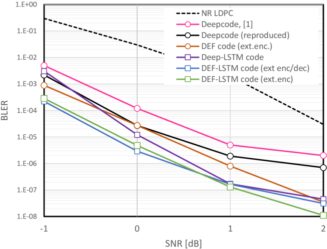
Figure 4: Performance comparison of Deepcode, DEF codes, LSTM-based Deepcode, and DEF-LSTM codes. Spectral efficiency is 0.67 bits/s/Hz ($Q=2$, $P=2$).

IV Performance Evaluations

In this section, we assess the BLER performance of DEF codes and compare their performance with the performance of the NR LDPC code reported in [12] and the performance of Deepcode [1] for the same spectral efficiency (SE). The SE is defined as the ratio of the number of information bits $L$ over the number of forward-channel time-frequency resources used for transmission of the corresponding codeword. As each time-frequency resource carries a complex symbol, and since each complex symbol is produced by combining two consecutive real symbols, we have

$$SE\triangleq\frac{Q}{1+P}\;\rm[bits/s/Hz].$$ (34)

The forward-channel and feedback-channel impairments are modeled as AWGN with variance $\sigma_{n}^{2}=1/{SNR}$ and $\sigma_{FB}^{2}=1/{SNR_{FB}}$, respectively. The training forward SNR and LLS forward SNR are the same; the feedback channel is noiseless.

The set of parameters used in the performance evaluations is shown in Table IV. For DEF code performance evaluations, we show that even the shortest feedback extensions – corresponding to the $\delta$ and $\gamma$ parameters of Table IV – produces significant gains. The investigation of performance with larger feedback extensions is left for future work. Details of the evaluated architectures are reported in Table V.

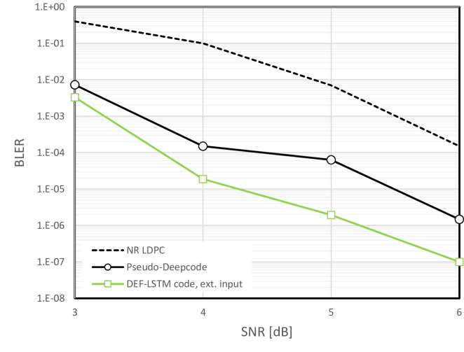
Figure 5: Performance comparison of Deepcode, pseudo-Deepcode, and DEF-LSTM code with extended encoder input. Spectral efficiency is 1.33 bits/s/Hz ($Q=4$, $P=2$).

DEF code parameter	Selected values
$K$ [symbols]	50
$P$	2
$H_{0}$	50
# zero-padding bits	1
Encoder input extensions	$(\delta_{0},\delta_{1},\delta_{2})=(1,2,2)$
Decoder input extensions	$(\gamma_{0},\gamma_{1},\gamma_{2})=(1,1,1)$

TABLE IV: Evaluation parameters.

Code	Encoder NN	Decoder NN
	(type, #layers)	(type, #layers)
Deepcode	RNN, 1	bidir. GRU, 2
DEF code	RNN, 1	bidir. GRU, 2
Deep-LSTM code	LSTM, 1	bidir. LSTM, 2
DEF-LSTM code	LSTM, 1	bidir. LSTM, 2

TABLE V: Evaluated architectures.

Fig. 4 shows the Block Error Rate (BLER) vs. forward SNR of several codes with $SE=0.67$ bits/s/Hz. The plot shows Deepcode [1] (pink curve), Deepcode obtained by the training method of Sec. III (solid black curve), DEF code with extended encoder input (orange curve), Deepcode with LSTM-based encoder and decoder NNs (purple curve), DEF code with extended encoder input (green curve) and DEF code with extended encoder and decoder input (blue curve). All DNN-based codes use second-order modulation (i.e., $Q=2$) and $P=2$ parity symbols per systematic symbol. Thus, the corresponding SE is $0.67$ bits/s/Hz. The performance of the NR LDPC code as reported in [12] with the same SE (QPSK modulation, code rate 1/3) is shown by a dashed black curve.

Based on the data shown in Fig. 4, the following observations are made:

• The DEF code with extended encoder input (orange curve) has better performance than Deepcode (solid black curve);

• The DEF-LSTM codes (green and blue curves) have the best performance among all the evaluated codes;

• DEF-LSTM code with extended encoder input and DEF-LSTM code with extended encoder/decoder input have similar performance except for high SNRs, where the former performs slightly better;

• DEF-LSTM codes (green and blue curve) outperform NR LDPC (dashed black curve) by at least three orders of magnitude BLER for all SNRs.

• The training method of Section III (black curve) produces codes with better performance than the training method of [1] (pink curve).

Based on the first observation above, it can be concluded that encoder input extension produces performance improvements. Subsequent observations highlight that the encoder input extension provides performance improvements when combined with LSTM. However, based on the observation in the third bullet, we can conclude that decoder input extension brings no benefits compared to encoder input extension. Moreover, the above performance evaluations show that usage of LSTM in the encoder and decoder provides significant performance improvements compared to RNN/GRU based codes.

Figure 5 shows the BLER performance of DNN-based codes with modulation order $Q=4$ – the corresponding SE is $1.33$ bits/s/Hz. As Deepcode [1] is not defined for SEs higher than $0.67$ bits/s/Hz, we implemented a pseudo-Deepcode by replacing the Deepcode modulator with a modulator of order $Q=4$. Results show that the DEF-LSTM code has better performance compared to the pseudo-Deepcode as its BLER is significantly lower in the whole range of SNR that we evaluated. The DEF-LSTM code BLER gain over pseudo-Deepcode is larger than one order of magnitude for SNR=5 dB and 6 dB. Moreover, the DEF-LSTM code outperforms NR LDPC (dashed black curve) by at least three orders of magnitude BLER for SNR $\geq 4$ dB.

V Conclusion and further work

A new deep-neural-network based error correction encoder architecture for channels with feedback has been presented. It has been shown that the codes designed according to the DEF architecture achieve lower error rates than any other code designed for channels with feedback. Moreover, by a suitable selection of the modulation order, these codes can adapt to the forward channel quality, thereby providing the maximum spectral efficiency that is attainable for the given forward channel quality.

Study of these codes in more realistic scenarios such as noisy feedback channels and fading is left for future work.

References

- [1] H. Kim, Y. Jiang, S. Kannan, S. Oh, P. Viswanath, “Deepcode: feedback codes via deep learning,” IEEE Journal on Selected Areas in Information Theory, vol. 1, no. 1, pp. 194-206, May 2020.
- [2] E. Arikan, “Channel polarization: a method for constructing capacity-achieving codes for symmetric binary-input memoryless channels,” IEEE Transactions on Information Theory, vol. 55, no. 7, pp. 3051-3073, July 2009.
- [3] D. J. C. MacKay, “Good error correcting codes based on very sparse matrices”, IEEE Transactions on Information Theory, vol. 45, no. 2, pp. 399-431, Mar. 1999.
- [4] C. Berrou, A. Glavieux and P. Thitimajshima, “Near Shannon limit error-correcting coding and decoding: turbo-codes,” International Conference on Communications, ICC’93,Geneva, Switzerland, pp. 1064-70, May 1993.
- [5] S. Lin, D. Costello, Error Control Coding, Prentice-Hall, Englewood Cliffs, NJ: 1983, 2011.
- [6] Y. Polyanskiy, H. V. Poor and S. Verdú, “Feedback in non-asymptotic regime,” IEEE Transactions on Information Theory,, vol. 57, no. 8, pp. 4903-4925, Aug. 2011.
- [7] J. Schalkwijk, “A coding scheme for additive noise channels with feedback-I: No bandwidth constraint,” IEEE Transactions on Information Theory, vol. 12, no. 2, pp. 172-182, Aug. 1966.
- [8] M. Horstein, “Sequential transmission using noiseless feedback,” IEEE Transactions on Information Theory, vol. 9, no. 3, pp. 136-143, July 1963.
- [9] J. M. Ooi and G. W. Wornell, “Fast iterative coding techniques for feedback channels,” IEEE Transactions on Information Theory,, vol. 44, no. 7, pp. 2960-2976, Nov. 1998.
- [10] Z. Ahmad, Z. Chance, D. J. Love and C. Wang, “Concatenated coding using linear schemes for Gaussian broadcast channels with noisy channel output feedback,” IEEE Transactions on Communications, vol. 63, no. 11, pp. 4576-4590, Nov. 2015.
- [11] K. Vakilinia, S. V. S. Sudarsan, V. S. Ranganathan, D. Divsalar and R. D. Wesel, “Optimizing transmission lengths for limited feedback with non-binary LDPC examples,” IEEE Transaction on communications,, vol. 64, no. 6, pp. 2245-2257, June 2016.
- [12] Huawei, HiSilicon, “Performance evaluation of LDPC codes for NR eMBB data,” 3GPP RAN1 meeting #90, Prague, Czech Republic, August 21–25, 2017.