Dirac-Born-Infeld warm inflation realization in the strong dissipation regime

Abstract

We consider warm inflation with a Dirac-Born-Infeld (DBI) kinetic term in which both the nonequilibrium dissipative particle production and the sound speed parameter slow the motion of the inflaton field. We find that a low sound speed parameter removes, or at least strongly suppresses, the growing function appearing in the scalar of curvature power spectrum of warm inflation, which appears due to the temperature dependence in the dissipation coefficient. As a consequence of that, a low sound speed helps to push warm inflation into the strong dissipation regime, which is an attractive regime from a model building and phenomenological perspective. In turn, the strong dissipation regime of warm inflation softens the microscopic theoretical constraints on cold DBI inflation. The present findings, along with the recent results from swampland criteria, give a strong hint that warm inflation may consistently be embedded into string theory.

I Introduction

Warm inflation (WI) Berera:1995wh ; Berera:1995ie ; Berera:1998px is an alternative dynamical realization for conventional cold inflation (CI) Guth:1980zm ; Sato:1981ds ; Albrecht:1982wi ; Linde:1981mu ; Linde:1983gd during which the inflaton field dissipates its vacuum energy into an ambient radiation bath, thus eliminating the necessity of a postinflationary reheating process Berera:1996fm and leading into different possibilities for a graceful exit mechanism Das:2020lut . Such a nonequilibrium dissipative particle production process acts to slow the motion of the inflaton field, allowing the embedding of steeper potentials in the WI context and helping to solve, for example, the so-called $\eta$-problem Berera:1999ws ; BasteroGil:2009ec ; Bastero-Gil:2019gao . In WI the thermal fluctuations play the dominant role in the formation of the seeds for the large scale structure (LSS) by producing a quasi scale-invariant spectrum of primordial curvature perturbations. At the same time, the shape of the produced spectrum depends on the field content of the model, leading to signatures able to make it distinguishable from the one produced in CI Bastero-Gil:2014raa ; Moss:2011qc ; Moss:2007cv ; Bastero-Gil:2014jsa ; Ramos:2013nsa ; BasteroGil:2011xd ; Graham:2009bf ; Hall:2003zp ; Bastero-Gil:2014oga . Furthermore, the rich dynamics of WI allows it to address/alleviate some of long-lasting problems related to the (post-)inflationary phase in the CI scenarios Bartrum:2012tg ; Sanchez:2010vj ; Motaharfar:2021gwi ; Bastero-Gil:2016mrl ; BasteroGil:2011cx ; Rosa:2019jci ; Dimopoulos:2019gpz ; Levy:2020zfo ; Rosa:2018iff ; Lima:2019yyv ; Sa:2020fvn ; Berghaus:2019cls (see also Refs. Dymnikova:1998ps ; Dymnikova:2001ga ; Dymnikova:2001jy for related work).

Despite its tremendous success, earlier particle physics realizations of WI were confronted with two important difficulties. The first one was that achieving a thermal radiation bath during inflation can result in potentially large thermal corrections to the inflaton’s potential, thus, hindering the slow-roll dynamics. Earlier WI model building constructions circumventing this problem made use of models with large field multiplicities Moss:2006gt ; BasteroGil:2010pb ; BasteroGil:2012cm ; Bartrum:2013fia , making them technically unappealing. This issue was later resolved with the introduction of a new class of WI model building realization able to sustain a nearly-thermal bath, yet with a small number of field species Bastero-Gil:2016qru . These type of models were dubbed “warm little inflaton (WLI)” models. The second difficulty was that the backreaction of the thermal radiation bath on the inflaton power spectrum due to a temperature dependent dissipation coefficient leads to the appearance of growing/decreasing modes in the scalar of curvature power spectrum Graham:2009bf . As a consequence of this, consistency with the observations could only be achieved in weak dissipation regimes of WI, thus preventing WI from going into a strong dissipation regime. However, the strong dissipation regime of WI is particularly appealing from both a theoretical and effective field theory point of view. In particular, the strong dissipation regime of WI can naturally result in a smaller energy scale inflation with sub-Planckian field excursions. These are features that have been attracting considerable attention, especially more recently, e.g., based on the swampland program aiming at finding effective field theories which can consistently be embedded in quantum gravity theories and the role played by WI in achieving this goal Das:2020xmh ; Brandenberger:2020oav ; Goswami:2019ehb ; Berera:2019zdd ; Kamali:2019xnt ; Das:2019hto ; Das:2018rpg ; Motaharfar:2018zyb . This issue was also partially addressed recently by building two distinct explicit WI models, namely the “variant of warm little inflaton” (VWLI) Bastero-Gil:2019gao and the “minimal warm inflation” (MWI) Berghaus:2019whh ; Laine:2021ego , utilizing different field contents in each construction. In the VWLI, the strong dissipative regime is obtained by interpolating between decreasing and growing modes, while in the MWI it is achievable only for some particular form of potentials, while growing/decreasing modes for the power spectrum can still exist in both cases.

As far as well-motivated theoretical field theory constructions for inflation are concerned, there has been considerable progress towards this goal in recent years, with the construction of several concrete string inflation models for instance (for reviews, see, e.g., Refs. Kallosh:2007ig ; Baumann:2009ni and references therein), with particular attention given to brane inflation scenarios. Dirac-Born-Infeld (DBI) inflation is one such string theoretic motivated model in which the inflaton is interpreted as a modulus parameter of a D-brane propagating in a warped throat region of an approximate Calabi-Yau flux compactification Silverstein:2003hf ; Alishahiha:2004eh . Hence, the effective action for DBI inflation contains a special form of the DBI kinetic term. The DBI kinetic term introduces some novel speed limits on the inflaton field velocity and helps in keeping it near the top of potential, even when it is too steep, thus resulting in the slow-roll phase through a low sound speed, instead of from dynamical friction due to expansion. A low sound speed, smaller than unity, allows the inflaton field to have a sub-Planckian evolution, even for steep potentials, thus circumventing the $\eta$-problem Easson:2009kk . Moreover, fluctuations also propagate with a low sound speed parameter, resulting in both a smaller tensor-to-scalar ratio and a significant non-Gaussianity, which can potentially be distinguishable from other scenarios Silverstein:2003hf ; Alishahiha:2004eh .

Although DBI inflation models were greatly successful, it was realized that the microscopic bound on the maximal field variation due to compactification is able to put strong constraints on the throat volume Baumann:2006cd and bulk volume Chen:2006hs . These issues, together with the Lyth bound, lead to a model independent upper bound on the tensor-to-scalar ratio which turns out to be inconsistent with the stringent observational lower bound on gravitational waves that are produced by the inflationary dynamics Lidsey:2007gq . Moreover, a viable reheating process, which typically involves brane/antibrane annihilation (see, e.g., Refs. Barnaby:2004gg ; Frey:2005jk ; Chialva:2005zy ; Firouzjahi:2005qs for earlier studies on reheating in brane inflation), is highly constrained due to overproduction of long-lived Kaluza-Klein (KK) modes Kofman:2005yz (note, however, that subsequently Refs. Chen:2006ni ; Berndsen:2008my ; Dufaux:2008br ; Frey:2009qb argued that warped KK modes can instead serve as dark matter candidates).

Reference Cai:2010wt showed that the cold DBI inflation model can be reconciled with the observations, removing the aforementioned inconsistencies, provided that the strong dissipation regime of Dirac-Born-Infeld warm inflation (DBIWI) is achieved. This is also because the WI scenario violates the Lyth bound. However, the work done in Ref. Cai:2010wt made use of a phenomenological dissipation coefficient, assuming it to be independent of the temperature. However, almost all explicit particle physics realizations of WI result in an explicit temperature dependent dissipation coefficient Berera:2008ar ; BasteroGil:2010pb ; BasteroGil:2012cm ; Bastero-Gil:2016qru ; Bastero-Gil:2019gao ; Berghaus:2019whh . Besides this, pushing WI into the strong dissipation regime is challenging due, again, to the aforementioned problem related to the appearance of a growing/decreasing function in the power spectrum, which tends to lead to results inconsistent with the observations, e.g., for the spectral tilt Benetti:2016jhf . Although there have been some previous papers considering DBIWI realizations Cai:2010wt ; Zhang:2014dja ; Rasouli:2018kvy , none of them made an investigation of the role of the sound speed on the backreaction of the radiation perturbations on the inflaton ones. Thus, none of the earlier references on DBIWI have studied how the growing/decreasing function in WI gets affected by the sound speed, which requires a detailed study of the perturbations in DBIWI. Taken all together, the purpose of this paper is to cover this issue and to properly understand the primordial perturbations in DBIWI and the consequences that it brings to model realizations, as far as the observations constraints are taken into account. Our results show that DBIWI is able to go into the strong dissipation regime for well-motivated field theory realizations of WI that result in explicit temperature dependent dissipation coefficients. Our results also shed new light on the potential use of DBI type of models in the context of WI.

The outline of the remainder of this paper is as follows. In Sec. II, we present the dynamics of DBIWI realization and investigate the behavior of the dynamical parameters in the model. Then, in Sec. III, we study the perturbation equations for the DBIWI and present the backreaction of the thermal radiation bath on the inflaton perturbations and scalar of curvature power spectrum. In Sec. IV we discuss the results obtained for the DBIWI and demonstrate the effect of a low sound speed on the spectrum of DBIWI. Finally, in Sec. V, we give a summary of the results and conclude by discussing the implications of the DBIWI realization from a model building perspective. Throughout this paper, we work with the natural units, in which Planck’s constant, the speed of light and Boltzmann’s constant are set to $1$ and we also work with the reduced Planck mass, $M_{\rm Pl}\equiv 1/\sqrt{8\pi G}\simeq 2.4\times 10^{18}$GeV.

II DBIWI background dynamics

The dynamical realization of WI is different from the CI one due to the presence of radiation and energy exchange between the inflaton field and the radiation energy density. Hence, the total energy density of the Universe in WI contains both the inflaton field and a primordial radiation energy density, i.e., $\rho=\rho_{\phi}+\rho_{r}$, where $\rho_{\phi}$ and $\rho_{r}$ are the inflaton field and the radiation energy densities, respectively. Even when $\rho_{r}$ is subdominated at the beginning and throughout inflation, i.e., $\rho_{r}\ll\rho_{\phi}$, the underlying dissipation effects generating this radiation energy density are still able to modify the inflationary dynamics and the perturbations in a nontrivial way in WI. The inflaton field and radiation energy density form a coupled system in the WI dynamics due to dissipation of energy out of the inflaton system and into radiation. In the spatially flat Friedmann-Lemaître-Robertson-Walker (FLRW) metric, the background evolution equations are, respectively, given by

$$\dot{\rho}_{\phi}+3H(\rho_{\phi}+p_{\phi})=-\Upsilon\left(\rho_{\phi}+p_{\phi}\right),$$ (1)

$$\dot{\rho}_{r}+3H(\rho_{r}+p_{r})=\Upsilon\left(\rho_{\phi}+p_{\phi}\right),$$ (2)

where $p_{\phi}$ and $p_{r}$ are the inflaton and radiation pressures, respectively, and $\Upsilon$ is the dissipation coefficient, which in general can be a function of both the inflaton field $\phi$ and temperature $T$ of the produced radiation bath.

In the DBIWI realization, the inflaton is a modulus parameter of a D-brane moving in a warped throat region which dissipates its vacuum energy into radiation through Eqs. (1) and (2), while its evolution is effectively governed by the following Lagrangian density,

$$\mathcal{L}_{DBI}=f^{-1}(\phi)\left[1-\sqrt{1-2f(\phi)X}\right]-V(\phi),$$ (3)

where $X=-\frac{1}{2}\partial^{\mu}\phi\partial_{\mu}\phi$, with $V(\phi)$ being the potential function for the inflaton and $f(\phi)$ is the redefined warp factor. The form for the warp factor function can be phenomenologicaly deformed depending on the desired model construction. For the well-studied anti-de Sitter throat Silverstein:2003hf ; Alishahiha:2004eh the warp factor function is given by $f(\phi)={f_{0}}/{\phi^{4}}$ with $f_{0}$ being a positive constant. For definiteness, this is the form for the warp factor function that we will be assuming in this work.

Varying the action with respect to the metric, the energy density $\rho_{\phi}$ and the pressure $p_{\phi}$ of the DBI field are given, respectively, by

$$\rho_{\phi}=\frac{\dot{\phi}^{2}}{c_{s}(1+c_{s})}+V(\phi),$$ (4)

$$p_{\phi}=\frac{\dot{\phi}^{2}}{1+c_{s}}-V(\phi),$$ (5)

where $c_{s}\equiv\sqrt{1-2Xf(\phi)}=\gamma^{-1}$ is the sound speed, which is smaller than unity as a consequence of the nontrivial kinetic structure of the DBI Lagrangian, with $\gamma$ similarly being the Lorentz factor in five dimensions. Inserting Eq. (4) in Eqs. (1) and (2), the dynamical equation for the inflaton field in the DBIWI is found to be given by

$$\ddot{\phi}+3c_{s}^{2}H(1+Q)\dot{\phi}+c_{s}^{3}V^{\prime}+\frac{f^{\prime}}{2f^{2}}\left(1-3c_{s}^{2}+2c_{s}^{3}\right)=0,$$ (6)

while for the radiation energy density is

$$\dot{\rho}_{r}+4H\rho_{r}=c_{s}^{-1}\Upsilon{\dot{\phi}^{2}},$$ (7)

where $Q=\Upsilon/(3H)$ gives a measure for the strength of the dissipative processes in WI. Equation (6) for the inflaton background evolution can also be obtained from the following covariant equation (when taking $\phi$ as an homogeneous field),

$$c_{s}^{-1}\Box\phi-c_{s}^{-3}f(\phi)(\nabla_{\mu}\nabla_{\nu}\phi)(\nabla^{\mu}\phi\nabla^{\nu}\phi)-V^{\prime}$$

$$-\frac{f^{\prime}(\phi)}{2f^{2}(\phi)}\left(c_{s}^{-3}-3c_{s}^{-1}+2\right)=-c_{s}^{-1}\Upsilon u^{\mu}\partial_{\mu}\phi.$$ (8)

In the slow-roll regime, $\ddot{\phi}\ll H\dot{\phi}$ and $\dot{\rho}_{r}\ll 4H\rho_{r}$, i.e., the inflaton is slowly varying and radiation is produced in a quasistationary way. Both slow-roll conditions hold as long as

$$\epsilon_{s}\equiv\frac{d\ln c_{s}}{dN}=\frac{\dot{c}_{s}}{Hc_{s}}\ll 1,$$ (9)

with $\epsilon_{s}$ quantifying the variation of the sound speed, along with the usual condition that the standard slow-roll parameters in WI are small. Then, under the slow-roll approximation, the background equations reduce to

$$\dot{\phi}\simeq-\frac{c_{s}V^{\prime}}{3H(1+Q)},\ \ \rho_{r}\simeq\frac{3Q\dot{\phi}^{2}}{4c_{s}},\ \ 3H^{2}\simeq\frac{V(\phi)}{M_{\rm Pl}}.$$ (10)

To study the model quantitatively, we need to fix the functionality of the potential and of the dissipation coefficient. In this paper, we consider a monomial power-law potential for the inflaton,

$$V(\phi)=\frac{V_{0}}{2n}\left(\frac{\phi}{M_{\rm Pl}}\right)^{2n},$$ (11)

where $V_{0}$ is the amplitude of the potential and $n$ is a real number. Moreover, the dissipation coefficient can be very well parameterized by

$$\Upsilon(\phi,T)=C_{\Upsilon}\,T^{c}\phi^{p}M^{1-p-c},$$ (12)

where $C_{\Upsilon}$ is a constant, $T$ is the temperature, $M$ is some appropriate mass scale and both quantities can be associated with the specifics of the microscopic model parameters leading to Eq. (12) (see, e.g., Refs. Gleiser:1993ea ; Berera:1998gx ; Berera:2008ar ; BasteroGil:2012cm ; Bastero-Gil:2016qru ; Laine:2021ego for some explicit examples of quantum field theory model derivations for dissipation coefficients used in WI).

The scalar of the curvature power spectrum in WI Graham:2009bf ; BasteroGil:2011xd ; Bastero-Gil:2014jsa ; Ramos:2013nsa has strong dependence on the dissipation ratio $Q$ and on the temperature over the Hubble parameter ratio, $T/H$. One also notes that strictly speaking $T/H$ can also be considered as a function of $Q$, once we use the CMB amplitude value to constrain the scalar power spectrum. In this case, $Q$ can be considered the relevant quantity parametrizing the WI dynamics. It is then useful to look at the dynamical behavior of these quantities during inflation. In particular, the analysis of their behavior is important to determine regimes where the spectral tilt of the scalar of curvature power spectrum increases (leading potentially to a blue-tilted spectrum) or decreases (and that can lead to a red-tilted spectrum). Such an analysis is particularly relevant in modeling WI models and constraining them with the observations Benetti:2016jhf . Furthermore, since $Q$ appears explicitly in the slow-roll parameters of WI, the behavior of $Q$ during WI is important for determining regimes where the dynamics are consistent and can have a graceful exit Das:2020lut . In the case of DBIWI, the slow-roll coefficients also depend on the sound speed $c_{s}$, hence, for completeness, we also study its behavior here. During slow-roll we find that the dissipation ratio $Q$, the temperature over Hubble parameter $T/H$, and the sound speed $c_{s}$ in DBIWI evolve with the number of e-folds $N$, respectively, as

$$\frac{d\ln Q}{dN} = \frac{c_{s}\left\{\left[4+c(1+c_{s}^{2})\right]\epsilon_{V}-c(1+c_{s}^{2})\eta_{V}-(2c(1-c_{s}^{2})+4p)\kappa_{V}\right\}}{4-c+4Q+cc_{s}^{2}Q},$$ (13)

$$\frac{d\ln(T/H)}{dN} = \frac{c_{s}\left\{\left(6+c_{s}^{2}+5Q+c(-1+c_{s}^{2}Q)\right)\epsilon_{V}-(1+c_{s}^{2})(1+Q)\eta_{V}+\left[p(c_{s}^{2}Q-1)-2(1+Q)(1-c_{s}^{2})\right]\kappa_{V}\right\}}{(1+Q)(4-c+4Q+cc_{s}^{2}Q)},$$

$$\frac{d\ln c_{s}}{dN} = \frac{c_{s}(1-c_{s}^{2})\left\{(-4+c+cQ)\epsilon_{V}-(-4+c)(1+Q)\eta_{V}-2\left[4-c+(4+c+2p)Q\right]\kappa_{V}\right\}}{(1+Q)(4-c+4Q+cc_{s}^{2}Q)},$$ (15)

where $\epsilon_{V}=M_{\rm Pl}^{2}(V^{\prime}/V)^{2}/2$ and $\eta_{V}=M_{\rm Pl}^{2}V^{\prime\prime}/V$ are the usual slow-roll inflaton potential parameters and $\kappa_{V}=M_{\rm Pl}^{2}V^{\prime}/(\phi\,V)$.

We note from Eqs. (13)-(15) that the denominator of those expressions is always positive. This is because the power $c$ in the temperature dependence of the dissipation coefficient satisfies $-4<c<4$ (see, e.g., Refs. Moss:2008yb ; delCampo:2010by ; BasteroGil:2012zr ). On the other hand, the sign of the numerator in the above expressions will depend on both the form of the dissipation coefficient and on the inflaton potential exponent $n$. As examples of representative cases of WI models, we can consider two cases of dissipation coefficient that are well motivated microscopically: (a) $c=1,\,p=0$, i.e., a linear in the temperature dependence for the dissipation coefficient, $\Upsilon\propto T$, that was first derived in Ref. Bastero-Gil:2016qru in the case of the WLI; and (b) $c=3,\,p=0$, i.e., a cubic power in the temperature dependence for the dissipation coefficient, $\Upsilon\propto T^{3}$, and derived recently in Refs. Berghaus:2019whh ; Laine:2021ego in the case of the MWI. From the Eqs. (13)-(15) we find that in case (a) both $Q$ and $T/H$ are growing functions with the number of e-folds for $n>1/3$ for all $c_{s}$, while $c_{s}$ initially decreases for $n<3$ when $Q\ll 1$, and for $Q>1$ it will increase for $n>13/7$ and decreases otherwise. In case (b) $Q$ and $c_{s}$ are decreasing functions with the number of e-folds whenever $n<3$ and $c_{s}^{2}<1/3$ or $n>3$ and $c_{s}^{2}>1/3$ and increasing functions with $N$ otherwise, while $T/H$ is in general a growing function with $N$. Both cases (a) and (b) then reinforce the WI condition $T/H>1$ throughout the inflationary dynamics.

III Perturbations for DBIWI

Let us describe the scalar perturbation equations in DBIWI. We start with the fully perturbed FLRW metric,

$$ds^{2} = -(1+2\alpha)dt^{2}-2a\partial_{i}\beta dx^{i}dt$$ (16)

$$+ a^{2}[\delta_{ij}(1+2\varphi)+2\partial_{i}\partial_{j}\gamma]dx^{i}dx^{j},$$

where $\alpha$, $\beta$, $\gamma$ and $\varphi$ are the spacetime-dependent metric perturbation variables. In WI the evolution of field fluctuations $\delta\phi$, which is effectively described by a stochastic evolution, is determined by a Langevin-like equation Graham:2009bf ; Bastero-Gil:2014jsa . In the case of DBIWI, perturbing the covariant equation (II) around the background, i.e., $\Phi({\bf x},t)=\phi(t)+\delta\phi({\bf x},t)$, the corresponding Langevin equation for $\delta\phi$ reads

$$\delta\ddot{\phi} +3H\ \left(1+Q-\epsilon_{s}\right)\delta\dot{\phi}+H^{2}\left\{z^{2}+\frac{3\dot{f}}{2Hf}\left[(1-c_{s}^{2})(1+Q)-\epsilon_{s}\right]-\frac{1-3c_{s}^{2}+2c_{s}^{3}}{H^{2}}\left(\frac{{f^{\prime}}^{2}}{f^{3}}-\frac{f^{\prime\prime}}{2f^{2}}\right)+\frac{c_{s}^{3}V^{\prime\prime}}{H^{2}}\right\}\delta\phi$$

$$+c_{s}^{2}\delta\Upsilon\dot{\phi}=c_{s}^{3}\left(\xi_{q}+\xi_{\Upsilon}\right)+\left[(3c_{s}^{-2}-1)\ddot{\phi}+3H(1+Q)\dot{\phi}\right]\alpha+(\dot{\alpha}+c_{s}^{2}\kappa)\dot{\phi}-\frac{3f^{\prime}}{2f^{2}}(1-c_{s}^{2})(1-c_{s}^{-2})\alpha,$$ (17)

which is also supplemented by the first-order perturbation equations for the radiation energy density, $\delta\rho_{r}$, and for the radiation momentum perturbation, $\Psi_{r}$, given, respectively, by

$$\delta\dot{\rho}_{r} +4H\delta\rho_{r}=\frac{k^{2}}{a^{2}}\Psi_{r}+\dot{\rho}_{r}\alpha+\frac{4}{3}\rho_{r}\kappa+\delta Q_{r},$$ (18)

and

$$\dot{\Psi}_{r} +3H\Psi_{r}=-\frac{\delta\rho_{r}}{3}-\frac{4}{3}\rho_{r}\alpha+J_{r}.$$ (19)

In the Eqs. (17), (18) and (19), we have that

$$\delta\Upsilon = 3HQ\left(\frac{c\delta{\rho_{r}}}{4\rho_{r}}+\frac{p\delta\phi}{\phi}\right),$$ (20)

$$\delta{Q}_{r} = c_{s}^{-1}\delta\Upsilon\dot{\phi}^{2}+3H^{2}Qc_{s}^{-3}(1-c_{s}^{2})\frac{\dot{f}}{2Hf}\dot{\phi}\delta\phi$$ (21)

$$+ 3c_{s}^{-3}(1+c_{s}^{2})HQ\dot{\phi}\delta\dot{\phi}$$

$$- 3c_{s}^{-3}(1+c_{s}^{2})HQ\dot{\phi}^{2}\alpha,$$

$$J_{r} = -c_{s}^{-1}\Upsilon\dot{\phi}\delta\phi,$$ (22)

where $z=c_{s}k/(aH)$, $\kappa=3(H\alpha-\dot{\varphi})+k^{2}\chi/a^{2}$ and $\chi=a(\beta+a\dot{\gamma})$. Moreover, in Eq. (17) $\xi_{q,\Upsilon}\equiv\xi_{q,\Upsilon}({\bf k},t)$ are stochastic Gaussian sources related to quantum and thermal fluctuations with appropriate amplitudes chosen such as to match the analytical derivation for the scalar of curvature power spectrum in WI Ramos:2013nsa . This leads in particular that $\xi_{\Upsilon}$ and $\xi_{q}$ both having zero mean and satisfying two-point correlation functions given, respectively, by

$$\!\!\!\!\!\!\!\!\!\!\langle\xi_{\Upsilon}({\bf k},t)\xi_{\Upsilon}({\bf k}^{\prime},t^{\prime})\rangle = \frac{2\Upsilon T}{a^{3}}\delta(t-t^{\prime})(2\pi)^{3}\delta({\bf k}+{\bf k}^{\prime}),$$ (23)

$$\!\!\!\!\!\!\!\!\!\!\langle\xi_{q}({\bf k},t)\xi_{q}({\bf k}^{\prime},t^{\prime})\rangle = \frac{H^{2}(9+12\pi Q)^{1/2}(1+2n_{*})}{\pi a^{3}}$$ (24)

$$\times \delta(t-t^{\prime})(2\pi)^{3}\delta({\bf k}+{\bf k}^{\prime}),$$

where $n_{*}$ represents the statistical distribution state for the inflaton quanta at the Hubble radius Ramos:2013nsa (see also the Appendix B of Ref. Das:2020xmh for details).

The set of perturbation equations (17), (18) and (19) are gauge-ready equations. They can be used with any appropriate gauge choice or also be worked out in terms of gauge-invariant quantities Kodama:1985bj ; Hwang:1991aj . For instance, they can be taken in the Newtonian-slicing (or zero-shear) gauge $\chi=0$, with the relevant metric equations becoming

$$\kappa=\frac{3}{2M_{\rm Pl}^{2}}(c_{s}^{-1}\dot{\phi}\delta\phi-\Psi_{r})\,,$$ (25)

$$\alpha=-\varphi\,,$$ (26)

$$\dot{\varphi}=-H\varphi-\frac{1}{3}\kappa\,.$$ (27)

It can also be easily checked that Eq. (17) reduces to the standard Langevin equation in WI Graham:2009bf ; Bastero-Gil:2014jsa for $c_{s}=1$, i.e., $\epsilon_{s}=0$. As it is clear from Eqs. (17) and (18), the term $\delta\Upsilon$ is responsible for coupling the inflaton perturbations with those of the radiation whenever $c\neq 0$ and which is known to lead to a growing mode for the resulting power spectrum Graham:2009bf .

III.1 The scalar of curvature power spectrum

Given the perturbation equations, Eqs. (17)-(19), the scalar power spectrum is determined from the comoving curvature perturbation ${\cal R}$,

$$\Delta_{\cal R}(k)=\frac{k^{3}}{2\pi^{2}}\langle|{\cal R}|^{2}\rangle\,,$$ (28)

where “$\langle\cdots\rangle$” means averaging over different realizations of the noise terms in Eq. (17) (see, for instance Refs. Graham:2009bf ; BasteroGil:2011xd ; Bastero-Gil:2014jsa for details of the numerical procedure). Given an appropriate gauge, ${\cal R}$ is composed of contributions from the inflaton momentum perturbations $\Psi_{\phi}=-c_{s}^{-1}\dot{\phi}\delta\phi$ and from the radiation momentum perturbations $\Psi_{r}$,

$${\cal R}=\sum_{i=\phi,r}\frac{\rho_{i}+p_{i}}{\rho+p}{\cal R}_{i}\;,$$ (29)

$${\cal R}_{i}=-\varphi-\frac{H}{\rho_{i}+p_{i}}\Psi_{i}\,,$$ (30)

with $p=p_{\phi}+p_{r}$, $\rho_{\phi}+p_{\phi}=c_{s}^{-1}\dot{\phi}^{2}$ and $\rho_{r}+p_{r}\simeq 4\rho_{r}/3=c_{s}^{-1}Q\dot{\phi}^{2}$.

An explicit analytic expression for the scalar of curvature power spectrum can be obtained when neglecting the coupling between inflaton and radiation perturbations (i.e., taking $c=0$ in Eq. (20)) and it was determined in Ref. Ramos:2013nsa . The result in this case is well approximated by Ramos:2013nsa

$$\Delta_{{\cal R}}\simeq\left(\frac{H_{*}^{2}}{2\pi\dot{\phi}_{*}}\right)^{2}\left(1+2{n_{BE}}+\frac{2\sqrt{3}\pi Q_{*}}{\sqrt{3+4\pi Q_{*}}}{T_{*}\over H_{*}}\right),$$ (31)

where $n_{BE}$ is the Bose-Einstein distribution and the effect of sound speed parameter is encoded in the inflaton field velocity through Eq. (10). One should note that in DBIWI, fluctuations are frozen at the sound horizon, where ${c_{s}}_{*}k_{*}=a_{*}H_{*}$, rather than at the Hubble radius, where $k_{*}=a_{*}H_{*}$. In general we can also replace $n_{BE}$ in Eq. (31) by $n_{*}$, representing the statistical distribution state of the inflaton at the sound horizon, which might not be necessarily that of thermal equilibrium. The form given by Eq. (31) is typically the result used in most of the recent literature in WI when the growing function is absent.

We want to first understand the effect of the coupling between inflaton and radiation perturbations and how a sound speed $c_{s}<1$ might change the results for the power spectrum in DBIWI. To possibly do something analytical and to obtain a feeling for these effects, we can start by considering some simplifying assumptions. Since we are interested in the strong dissipation regime $Q>1$, we can start by neglecting the contribution of quantum fluctuations to the power spectrum. For $Q>1$, the contribution from the thermal stochastic fluctuations $\xi_{\Upsilon}$ in Eq. (17) dominates over that from the quantum fluctuations $\xi_{q}$. Moreover, we can also analytically solve Eq. (17) explicitly by neglecting the slow-roll order corrections (and likewise the metric contributions, which also give slow-order corrections only). Under these simplifying assumptions, the authors in Ref. Graham:2009bf have explicitly shown that the power spectrum grows with $Q_{*}$ like $\Delta_{\mathcal{R}}\propto\Delta_{{\cal R},c=0}Q_{*}^{3c}$, with

$$\Delta_{{\cal R},c=0}\simeq\frac{\sqrt{3}}{4\pi^{\frac{3}{2}}}\frac{H^{3}_{*}T_{*}}{\dot{\phi}^{2}_{*}}Q_{*}^{\frac{1}{2}},$$ (32)

when taking $Q_{*}\gg 1$ in Eq. (31). By utilizing the same techniques developed in Ref. Graham:2009bf , but now adapted to the perturbation equations in DBIWI, we arrive at the result, when $Q_{*}\gg 1$, that $\Delta_{\mathcal{R}}$ is now given by

$$\Delta_{\mathcal{R}}\simeq\Delta_{{\cal R},c=0}\left(\frac{Q_{*}}{Q_{c}}\right)^{3cc_{s*}^{2}},$$ (33)

where $Q_{c}$ is a function of both $c$ and $c_{s}$. The result given by Eq. (33) explicitly shows that $c_{s}<1$ can compensate for the result of a growing scalar spectrum amplitude the larger is $Q$ and whenever $c>0$ (or, likewise, a decreasing amplitude when $c<0$). The approximations assumed in Ref. Graham:2009bf do allow us to solve for the inflaton perturbations and, hence, they help to find an analytical expression for $\Delta_{\mathcal{R}}$, it has been shown in Ref. BasteroGil:2011xd that these approximations tend to overestimate the effect of the coupling between the inflaton and radiation perturbations. By accounting for the full expressions, i.e., not dropping all slow-roll order terms in the equations, the dependence of $\Delta_{\mathcal{R}}$ on $Q_{*}$ tends to be more suppressed, with a smaller power in $Q_{*}$. Hence, the results from the (numerical) solution for the full perturbation equations shows that $\Delta_{\mathcal{R}}\propto Q_{*}^{\beta}$, with $\beta<3c$, when $c_{s}=1$. This result is also observed in our analysis shown in the next section, showing that $\beta<3cc_{s*}^{2}$ also holds here in the DBIWI. However, the effect is still large enough to make the spectrum to depart considerably from the result given by Eq. (31). By explicitly numerically solving the set of perturbations equations, as in Ref. BasteroGil:2011xd , the result of the coupling between inflaton and radiation perturbations can be expressed as an overall correction to Eq. (31), which modifies it to

$$\Delta_{{\cal R}}=\left(\frac{H_{*}^{2}}{2\pi\dot{\phi}_{*}}\right)^{2}\left(1+2n_{BE}+\frac{2\sqrt{3}\pi Q_{*}}{\sqrt{3+4\pi Q_{*}}}{T_{*}\over H_{*}}\right)G(Q_{*}),$$ (34)

where $G(Q_{*})$ accounts for the effect of the coupling of the inflaton and radiation fluctuations. Some explicit forms for $G(Q_{*})$ have been given in the literature, depending on the form of the dissipation coefficient in WI BasteroGil:2011xd ; Bastero-Gil:2014jsa ; Benetti:2016jhf ; Bastero-Gil:2016qru ; Motaharfar:2018zyb ; Kamali:2019xnt ; Lima:2019yyv ; Das:2020xmh . In the next section we will give results for $G(Q_{*})$ in the DBIWI case for some of the most representative dissipation coefficient forms used in recent literature and we will also explicitly see how a $c_{s}<1$ effectively suppresses the effects of a growing $Q_{*}$ in the amplitude of the scalar power spectrum. But before going into that analysis, let us also derive some useful results concerning the spectral tilt in DBIWI.

III.2 The spectral tilt $n_{s}$ in DBIWI

From Eq. (34) and also using Eqs. (13)-(15), we can explicitly find expressions for the spectral tilt $n_{s}$,

$$n_{s}-1=\frac{d\ln\Delta_{{\cal R}}(k)}{d\ln k}\simeq\frac{d\ln\Delta_{{\cal R}}(k)}{dN},$$ (35)

which in the weak and strong dissipation regimes of DBIWI are given, respectively, by

$$\left(n_{s}-1\right)\Bigr{|}_{Q_{*}\ll 1} = \frac{c_{s*}}{4-c}\left\{-\left[10+7c_{s*}^{2}-c(3+2c_{s*}^{2})\right]\epsilon_{V}\right.$$ (36)

$$+ \left.\left[-1+(7-2c)c_{s*}^{2}\right]\eta_{V}\right.$$

$$+ \left.\left[(14-4c)(1-c_{s*}^{2})-p\right]\kappa_{V}\right\},$$

and

$$\left(n_{s}-1\right)\Bigr{|}_{Q_{*}\gg 1} =-\frac{c_{s*}}{2(4+cc_{s*}^{2})Q_{*}}\left\{\left[18-c(1-c_{s*}^{2})\right]\epsilon_{V}\right.$$ (37)

$$\!\!\!\!\!\!\!+\left.\left[2+c+(-14+5c)c_{s*}^{2}\right]\eta_{V}\right.$$

$$\!\!\!\!\!\!\!+\left.2\left[c(1-c_{s*}^{2})+2(-7+p)+7(2+p)c_{s*}^{2}\right]\kappa_{V}\right\}$$

$$\!\!\!\!\!\!\!+\frac{c_{s*}}{4+cc_{s*}^{2}}\left\{\left(4+c+cc_{s*}^{2}\right)\epsilon_{V}-c(1+c_{s*}^{2})\eta_{V}\right.$$

$$\!\!\!\!\!\!\!-\left.\left[2c(1-c_{s*}^{2})+4p\right]\kappa_{V}\right\}\frac{G^{\prime}(Q_{*})}{G(Q_{*})}.$$

Note that in the case of the primordial inflaton potential of the form Eq. (11), we have in Eqs. (36) and (37) that

$$\epsilon_{V} = \frac{2n^{2}M_{\rm Pl}^{2}}{\phi_{*}^{2}},$$ (38)

$$\eta_{V} = \frac{2n(2n-1)M_{\rm Pl}^{2}}{\phi_{*}^{2}},$$ (39)

$$\kappa_{V} = \frac{2nM_{\rm Pl}^{2}}{\phi_{*}^{2}}.$$ (40)

In deriving the Eqs. (36) and (37) for $n_{s}$ we have also considered that in WI that $T_{*}/H_{*}\gg 1$ (in particular, $T_{*}/H_{*}\gg 1$ can be explicitly verified in the examples to be considered in the next section). Finally, in the regime $T_{*}/H_{*}\ll 1$ and $Q_{*}\ll 1$ we recover the cold inflation standard result, $n_{s}-1=-6\epsilon_{V}+2\eta_{V}$. We can note from Eq. (37) that when $c_{s*}\ll 1$, in the absence of the growing mode, $G^{\prime}(Q)\to 0$, we have that $n_{s}-1\propto-1/Q$ and the spectral tilt will tend to be red-tilted for large $Q$. However, in the presence of the growing mode, the last term in Eq. (37) dominates at large $Q$ and it will tend to drive the spectrum to be blue-tilted (for $G^{\prime}(Q)>0$). To better illustrate the latter case, let us consider a few relevant WI dissipation terms that have commonly been used in the literature, namely, (a) the linear in the temperature dissipation coefficient Bastero-Gil:2016qru , with $c=1,\,p=0$; (b) the cubic in the temperature dissipation coefficient, with $c=3,\,p=0$ (e.g., from Ref. Berghaus:2019whh ) and (c) the dissipation coefficient with $c=3,\,p=-2$ (see, e.g., Refs. BasteroGil:2012cm ; Bartrum:2013fia ). For definiteness, we will also consider the example of a primordial potential with a quartic inflaton potential ($n=2$), which has been the primordial potential mostly considered with these dissipation coefficients in WI. We will also assume that the growing mode function is well described by a polynomial function in the dissipation ratio $Q$, with the leading term for $Q\gg 1$ of the form $G(Q)\propto Q^{\beta}$. Let us see the results for each of these three cases separately.

III.2.1 Case (a)

For case (a), with $c=1,\,p=0$, we obtain for Eq. (37) that

$$\left(n_{s}-1\right)\Bigr{|}_{Q_{*}\gg 1}\simeq\frac{-2c_{s*}\left[(17+c_{s*}^{2})-2\beta(5+c_{s*}^{2})\right]}{(4+c_{s*}^{2})Q_{*}(\phi_{*}/M_{\rm Pl})^{2}}.$$ (41)

Hence, for $c_{s*}\ll 1$ we have that the spectral tilt will turn blue, i.e., $n_{s}-1>0$, if $\beta>1.7$, while for $c_{s*}=1$, the spectral tilt is blue for $\beta>1.5$. We recall that for this case Bastero-Gil:2016qru we have that $\beta\simeq 2.315$ (for $c_{s*}=1$), thus, for large $Q$ this dissipation coefficient with a quartic inflaton potential will always disagree with the observations. But from Eq. (33), we expect that $\beta$ will decrease proportional to $c_{s}^{2}$. Thus, we need at least $c_{s*}^{2}\lesssim 1.7/2.315\sim 0.7$ for the model to be able to sustain a large dissipation DBIWI regime and to have a red-tilted scalar of curvature power spectrum, consistent with the observations. This expectation will be confirmed by our numerical results shown in Sec. IV.

III.2.2 Case (b)

For case (b), with $c=3,\,p=0$, we obtain for Eq. (37) that

$$\left(n_{s}-1\right)\Bigr{|}_{Q_{*}\gg 1}\simeq\frac{-2c_{s*}\left[(23+31c_{s*}^{2})-2\beta(-1+3c_{s*}^{2})\right]}{(4+3c_{s*}^{2})Q_{*}(\phi_{*}/M_{\rm Pl})^{2}}.$$ (42)

Hence, for $c_{s*}\ll 1$ we have that the spectral tilt, different from the previous case, will always be red, since in this case $n_{s}-1\propto-(23+2\beta)$. When $c_{s*}=1$, we see from Eq. (42) that $n_{s}-1\propto-(54-4\beta)$ and the spectral tilt is, thus blue for $\beta>13.5$. But in this case Benetti:2016jhf we have that $\beta\simeq 4.33$ (for $c_{s*}=1$), hence, for large $Q$ this dissipation coefficient with a quartic inflaton potential can quite robustly sustain a red-tilted spectrum. In fact, the effect of having a $c_{s*}<1$ here can potentially make the spectrum too red tilted to be consistent with the observations, since a value of $c_{s*}<1$ would make the exponent $\beta$ smaller and lead to a redder spectrum. This is confirmed by our numerical results shown in Sec. IV. Since this type of dissipation coefficient already leads to quite satisfactory results when compared to the observations Berghaus:2019whh , even in the strong dissipation regime of WI, it does not benefit from a DBIWI construction, at least in the context of monomial chaotic inflaton potentials.

III.2.3 Case (c)

It is useful to compare case (b) with the results for case (c), when $c=3,\,p=-2$, in which case the dissipation coefficient depends on the temperature but also on the inflaton amplitude. In this case, we obtain for Eq. (37) that

$$\left(n_{s}-1\right)\Bigr{|}_{Q_{*}\gg 1}\simeq\frac{-2c_{s*}\left[3(5+c_{s*}^{2})-2\beta(7+3c_{s*}^{2})\right]}{(4+3c_{s*}^{2})Q_{*}(\phi_{*}/M_{\rm Pl})^{2}}.$$ (43)

Here, we have that for $c_{s*}\ll 1$ the spectral tilt is such that it will turn blue when $\beta>15/14\simeq 1.07$, while for $c_{s*}=1$, the spectral tilt is blue already for $\beta>0.9$. In this case we still have $\beta\simeq 4.33$ (for $c_{s*}=1$), thus, for large $Q$ the spectrum will always be quite blue tilted. This agrees with the previous results for this type of WI model Bartrum:2013fia ; Benetti:2016jhf , which have shown that this dissipation coefficient, within the mononial chaotic inflaton potential models, can only be consistent with the observational data when $Q_{*}\ll 1$, i.e., in the weak dissipation regime of WI. In this regime of $Q_{*}\ll 1$, the growing mode is not an issue, since $G(Q_{*})\to 1$. As in case (a) with a linear temperature dissipation coefficient, this model can benefit from a DBIWI realization by exploring the effect of a small $c_{s}$ value, which will help to suppress the growing mode by decreasing $\beta$. However, this is expected to only happen for a smaller value for $c_{s}$ than the one shown for the case (a), $c_{s*}^{2}\lesssim 0.2$. This case also illustrates well the importance in deriving the full dependence of the dissipation coefficient in both the temperature and in the inflaton field amplitude. Despite cases (b) and (c) have exactly the same temperature dependence, the fact that the dissipation coefficient in (c) has an explicit dependence on $\phi$, implies that an agreement with the observational value for the tilt of the scalar power spectrum can only be achieved in the weak dissipation regime of WI (for the standard case of $c_{s*}=1$), while in (b) we can robustly support the strong dissipation regime of WI, even with the presence of the growing mode ()which in that case is benign).

III.3 Non-Gaussianities in DBIWI

Before ending this section. Let us briefly comment on the expected non-Gaussianities in DBIWI. In the DBIWI realization, non-Gaussianities may be generated by both nonequilibrium dissipative effects and by a low sound speed. It was shown in Ref. Moss:2011qc ; Bastero-Gil:2014raa that non-Gaussianities produced by temperature dependent dissipation coefficients are larger than temperature independent dissipation coefficients due to the backreaction of radiation bath and coupling of the inflaton to the radiation field perturbations. However, we qualitatively expect that for low sound speeds, $c_{s*}<1$, a suppressing effect, as seen for the scalar of curvature power spectrum, will also work in the case of the nonlinear parameter $f_{NL}$. Moreover, the non-Gaussianity parameter for WI in the strong dissipation regime is roughly less than $10$, i.e., $|f_{NL}^{Warm}|\leq 10$, for temperature dependent dissipation coefficients Moss:2011qc ; Bastero-Gil:2014raa . Furthermore, the non-Gaussianity produced by cold DBI inflation is inversely proportional to the square of the sound speed, i.e., $f_{NL}\simeq\frac{35}{108}(c_{s}^{-2}-1)$. Hence, the corresponding non-Gaussianity parameter in cold DBI inflation is $f_{NL}\simeq 3$ for $c_{s*}=0.3$, which is not very large. Therefore, depending on how these two non-Gaussianity sources contribute to the non-Gaussianity parameter (where they can either counterbalance or enforce each other), we may obtain large or small non-Gaussianities in DBIWI Cai:2010wt ; Zhang:2014kwa . Nonetheless, a comprehensive analysis is needed to find how large the non-Gaussianity will be in the DBIWI realization.

IV Results

To demonstrate the effect of $c_{s}$ on the power spectrum in the DBIWI realization, more precisely on the function $G(Q_{*})$, we have considered the quartic monomial inflaton potential ($n=2$) and focused our studies for the two representative more recent cases of WI dissipation coefficients, namely, $\Upsilon=C_{\Upsilon}T$ and $\Upsilon=C_{\Upsilon}T^{3}/M^{2}$. Results for other cases of monomial inflaton potential are found to be very similar to the quartic one, so we refrain from showing those other cases with expected similar results here. The growing function $G(Q_{*})$ is determined by the numerical evaluation of the perturbation equations and obtaining the scalar of curvature power spectrum (28), with $G(Q_{*})$ defined as

$$G(Q_{*})=\frac{\Delta_{{\cal R},c\neq 0}}{\Delta_{{\cal R},c=0}},$$ (44)

where $\Delta_{{\cal R},c\neq 0}$ is the solution for the scalar of curvature power spectrum with the explicit coupling of the inflaton perturbations with the radiation ones in Eq. (17) and $\Delta_{{\cal R},c=0}$ is the solution when this coupling is explicitly dropped from the equation. We should note that during the numerical analysis, although we dropped the metric perturbations, which is justified in an appropriate gauge and in the strong dissipation regime, we take into account the effect of first order slow-roll parameters, i.e. $\epsilon_{V}$, $\eta_{V}$, $\kappa_{V}$, etc., in Eq. (17) to obtain the precise behavior for the growing function. The results for the linear and cubic dependencies in temperature for the dissipation coefficient are shown in Fig. 1. The results shown in Fig. 1 indicate that for $c_{s}\lesssim 0.1$ the growing function $G(Q_{*})$ can indeed be taken as $G(Q_{*})\approx 1$.

(a)  Linear in $T$ dissipation coefficient

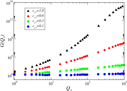
(b)  Cubic in $T$ dissipation coefficient

Figure 1: The growing function $G(Q_{*})$ as defined by Eq. (44).

As shown in the previous section, we may obtain a red-tilted spectral index in the strong dissipation regime even if $c_{s*}$ has intermediate values, not necessarily for values of $c_{s*}\ll 1$. This is because as $c_{s*}<1$, it can already suffice to suppress the growing mode enough to allow for a red-tilted spectrum, even for large $Q$ values. Thus small, but still reasonable values for $c_{s*}$ can work to allow the spectrum in DBIWI to be red-tilted in the strong dissipation regime. Hence, it is useful to obtain the exact functionality of $G(Q_{*})$ for future analysis. In this regard, we present the following fitting functions to the curves shown in Fig. 1,

$$G(Q_{*}) =1+A_{c}Q^{\alpha}_{*}+B_{c}Q^{\beta}_{*},$$ (45)

where the coefficients $\alpha$, $\beta$, $A_{c}$ and $B_{c}$ are given in the Table 1 for the two representative values of $c$ (i.e., for a linear and a cubic in $T$ dissipation coefficients, as obtained in the LWI and MWI models, respectively) and also for three representative values for $c_{s}$ (at the effective Hubble radius crossing).

Table 1: The coefficients $\alpha$, $\beta$, $A_{c}$ and $B_{c}$ in growing function $G(Q_{*})$ with different values for $c$ and $c_{s}$.

$c$	$c_{s*}$	$\alpha$	$\beta$	$A_{c}$	$B_{c}$
	1	1.364	2.315	0.335	0.0185
1	0.6	0.694	1.114	0.311	0.187
	0.3	0.395	0.448	0.205	0.127
	1	1.946	4.330	4.981	0.127
3	0.6	1.975	2.684	0.475	0.083
	0.3	0.815	0.939	0.478	0.368

When these results are applied to the cubic in the temperature form for the dissipation coefficient ($c=3,\,p=0$) and as already anticipated from the discussion given for case (b) in Sec. III.2.2, for values of $c_{s}<1$, we get that $n_{s}\simeq 0.95$ and even smaller values for $n_{s}$ the larger is $Q_{*}$ and the smaller is $c_{s*}$, showing that the spectrum is already outside the two-sigma range in the red-tilted side of the observational values for $n_{s}$. This indicates that for this form of a cubic dissipation coefficient, the model is not expected to benefit from a DBIWI realization, as already discussed before. Let us then next focus on the linear dissipation coefficient WI model of Ref. Bastero-Gil:2016qru . Some explicit examples of results obtained in this case are given in Table 2 for the quartic inflaton potential and with a linear in $T$ dissipation coefficient. As it is clear, for $Q_{*}>10$, the tensor-to-scalar ratio is smaller than $10^{-7}$, hence, the model is able to resolve the aforementioned inconsistency in the cold DBI inflation Lidsey:2007gq and discussed in the Introduction section.

Table 2: Numerical values of the parameters and the relevant cosmological quantities obtained for the case of a quartic inflaton potential ($n=2$) with a linear in $T$ dissipation coefficient ($c=1$, $p=0$) and for $c_{s*}=0.1$, when $G(Q_{*})=1$, and for $c_{s*}=0.3$, when $G(Q_{*})$ is given by Eq. (45).

$c_{s*}$	$Q_{*}$	$n_{s}$	$r$	$N_{*}$	$|\Delta\phi|/M_{\rm Pl}$	$C_{\Upsilon}$	$T_{\rm end}$ (GeV)	$V_{0}$ (GeV)4	$\epsilon_{V_{*}}$	$\eta_{V_{*}}$	$V_{*}^{1/4}/M_{\rm Pl}$	$f_{0}$
	1.03	0.9651	$1.13\times 10^{-5}$	62.1	3.36	0.0067	$2.67\times 10^{13}$	$3.94\times 10^{59}$	0.68	1.02	$1.56\times 10^{-5}$	$3.30\times 10^{17}$
0.1	10.25	0.9628	$3.00\times 10^{-7}$	61.0	1.42	0.023	$1.08\times 10^{13}$	$3.27\times 10^{59}$	3.80	5.71	$6.31\times 10^{-6}$	$2.14\times 10^{18}$
	102.51	0.9625	$3.88\times 10^{-9}$	60.0	0.46	0.076	$3.68\times 10^{12}$	$3.69\times 10^{59}$	35.55	53.33	$2.16\times 10^{-6}$	$1.71\times 10^{19}$
	1.03	0.9672	$3.33\times 10^{-5}$	62.4	5.85	0.0088	$3.27\times 10^{13}$	$1.27\times 10^{59}$	0.23	0.34	$1.91\times 10^{-5}$	$3.15\times 10^{17}$
0.3	10.30	0.9667	$5.70\times 10^{-7}$	61.5	2.44	0.027	$1.09\times 10^{13}$	$7.24\times 10^{58}$	$1.30$	1.95	$6.39\times 10^{-6}$	$2.91\times 10^{18}$
	103.16	0.9684	$3.49\times 10^{-9}$	60.3	0.79	0.074	$3.08\times 10^{12}$	$3.40\times 10^{58}$	12.31	18.47	$1.80\times 10^{-6}$	$4.73\times 10^{19}$

V Conclusions

We studied the effects of a low sound speed on the dynamics of perturbations equations of WI inspired by string motivated models that include relativistic D-brane motion. We numerically solved the coupled inflaton and radiation field perturbation equations for the first time in the case of a noncanonical kinetic term in DBIWI. We found that a low sound speed is able to suppress the growing function that always appears in the scalar power spectrum of WI, whenever the dissipation coefficient exhibits an explicit dependence with the temperature of the radiation bath. As a consequence of this suppression effect seen in DBIWI, the restrictions for constructing a WI realization in the strong dissipation regime $Q\gg 1$ are considerably relaxed. We have also complemented these results with the ones derived from the analytical expressions for the spectral tilt. Based on our results, as the low sound speed will push WI models into the strong dissipation regime, the severe inconsistency problems seen in DBI cold inflation, e.g., due to an upper bound on the tensor-to-scalar ratio arising from compactification constraints and a lower bound from observations, can all be resolved due to large dissipation. We have explicitly shown that among the most common dissipation coefficients that have been derived from well-motivated particle physics realizations and applied to the WI context, the dissipation coefficient with a linear dependence on the temperature is the case that can mostly benefit from a DBIWI realization. Hence, these type of models are able to soften all theoretical and observational constraints, while predicting very small tensor-to-scalar ratio and potentially significant non-Gaussianity, making them falsifiable in near future.

From a model-building perspective, the present work, along with the previous results on swampland conjectures in WI Kamali:2019xnt , gives a strong hint that WI may consistently be embedded in string theory utilizing the physics of the brane. Besides, phenomenologically realizing WI in the strong dissipation regime is a significant step towards achieving such goal. Therefore, the last step is building an explicit model describing how D-brane may be able to dissipate its energy into radiation field. This and other implications of our results are certainly worthwhile to explore further in future studies.

References

- (1) A. Berera and L. Z. Fang, “Thermally induced density perturbations in the inflation era,” Phys. Rev. Lett. 74, 1912-1915 (1995) doi:10.1103/PhysRevLett.74.1912 [arXiv:astro-ph/9501024 [astro-ph]].
- (2) A. Berera, “Warm inflation,” Phys. Rev. Lett. 75, 3218-3221 (1995) doi:10.1103/PhysRevLett.75.3218 [arXiv:astro-ph/9509049 [astro-ph]].
- (3) A. Berera, M. Gleiser and R. O. Ramos, “A First principles warm inflation model that solves the cosmological horizon / flatness problems,” Phys. Rev. Lett. 83, 264-267 (1999) doi:10.1103/PhysRevLett.83.264 [arXiv:hep-ph/9809583 [hep-ph]].
- (4) A. H. Guth, “The Inflationary Universe: A Possible Solution to the Horizon and Flatness Problems,” Phys. Rev. D 23, 347-356 (1981) doi:10.1103/PhysRevD.23.347
- (5) K. Sato, “Cosmological Baryon Number Domain Structure and the First Order Phase Transition of a Vacuum,” Phys. Lett. B 99, 66-70 (1981) doi:10.1016/0370-2693(81)90805-4
- (6) A. Albrecht and P. J. Steinhardt, “Cosmology for Grand Unified Theories with Radiatively Induced Symmetry Breaking,” Phys. Rev. Lett. 48, 1220-1223 (1982) doi:10.1103/PhysRevLett.48.1220
- (7) A. D. Linde, “A New Inflationary Universe Scenario: A Possible Solution of the Horizon, Flatness, Homogeneity, Isotropy and Primordial Monopole Problems,” Phys. Lett. B 108, 389-393 (1982) doi:10.1016/0370-2693(82)91219-9
- (8) A. D. Linde, “Chaotic Inflation,” Phys. Lett. B 129, 177-181 (1983) doi:10.1016/0370-2693(83)90837-7
- (9) A. Berera, “Interpolating the stage of exponential expansion in the early universe: A Possible alternative with no reheating,” Phys. Rev. D 55, 3346-3357 (1997) doi:10.1103/PhysRevD.55.3346 [arXiv:hep-ph/9612239 [hep-ph]].
- (10) S. Das and R. O. Ramos, “On the graceful exit problem in warm inflation,” [arXiv:2005.01122 [gr-qc]].
- (11) A. Berera, “Warm inflation at arbitrary adiabaticity: A Model, an existence proof for inflationary dynamics in quantum field theory,” Nucl. Phys. B 585, 666-714 (2000) doi:10.1016/S0550-3213(00)00411-9 [arXiv:hep-ph/9904409 [hep-ph]].
- (12) M. Bastero-Gil and A. Berera, “Warm inflation model building,” Int. J. Mod. Phys. A 24, 2207-2240 (2009) doi:10.1142/S0217751X09044206 [arXiv:0902.0521 [hep-ph]].
- (13) M. Bastero-Gil, A. Berera, R. O. Ramos and J. G. Rosa, “Towards a reliable effective field theory of inflation,” Phys. Lett. B 813, 136055 (2021) doi:10.1016/j.physletb.2020.136055 [arXiv:1907.13410 [hep-ph]].
- (14) M. Bastero-Gil, A. Berera, I. G. Moss and R. O. Ramos, “Theory of non-Gaussianity in warm inflation,” JCAP 12, 008 (2014) doi:10.1088/1475-7516/2014/12/008 [arXiv:1408.4391 [astro-ph.CO]].
- (15) I. G. Moss and T. Yeomans, “Non-gaussianity in the strong regime of warm inflation,” JCAP 08, 009 (2011) doi:10.1088/1475-7516/2011/08/009 [arXiv:1102.2833 [astro-ph.CO]].
- (16) I. G. Moss and C. Xiong, “Non-Gaussianity in fluctuations from warm inflation,” JCAP 04, 007 (2007) doi:10.1088/1475-7516/2007/04/007 [arXiv:astro-ph/0701302 [astro-ph]].
- (17) M. Bastero-Gil, A. Berera, I. G. Moss and R. O. Ramos, “Cosmological fluctuations of a random field and radiation fluid,” JCAP 05, 004 (2014) doi:10.1088/1475-7516/2014/05/004 [arXiv:1401.1149 [astro-ph.CO]].
- (18) R. O. Ramos and L. A. da Silva, “Power spectrum for inflation models with quantum and thermal noises,” JCAP 03, 032 (2013) doi:10.1088/1475-7516/2013/03/032 [arXiv:1302.3544 [astro-ph.CO]].
- (19) M. Bastero-Gil, A. Berera and R. O. Ramos, “Shear viscous effects on the primordial power spectrum from warm inflation,” JCAP 07, 030 (2011) doi:10.1088/1475-7516/2011/07/030 [arXiv:1106.0701 [astro-ph.CO]].
- (20) C. Graham and I. G. Moss, “Density fluctuations from warm inflation,” JCAP 07, 013 (2009) doi:10.1088/1475-7516/2009/07/013 [arXiv:0905.3500 [astro-ph.CO]].
- (21) L. M. H. Hall, I. G. Moss and A. Berera, “Scalar perturbation spectra from warm inflation,” Phys. Rev. D 69, 083525 (2004) doi:10.1103/PhysRevD.69.083525 [arXiv:astro-ph/0305015 [astro-ph]].
- (22) M. Bastero-Gil, A. Berera, R. O. Ramos and J. G. Rosa, “Observational implications of mattergenesis during inflation,” JCAP 10, 053 (2014) doi:10.1088/1475-7516/2014/10/053 [arXiv:1404.4976 [astro-ph.CO]].
- (23) S. Bartrum, A. Berera and J. G. Rosa, “Gravitino cosmology in supersymmetric warm inflation,” Phys. Rev. D 86, 123525 (2012) doi:10.1103/PhysRevD.86.123525 [arXiv:1208.4276 [hep-ph]].
- (24) J. C. Bueno Sanchez, M. Bastero-Gil, A. Berera, K. Dimopoulos and K. Kohri, “The gravitino problem in supersymmetric warm inflation,” JCAP 03, 020 (2011) doi:10.1088/1475-7516/2011/03/020 [arXiv:1011.2398 [hep-ph]].
- (25) M. Motaharfar and P. Singh, “On the role of dissipative effects in the quantum gravitational onset of warm Starobinsky inflation in a closed universe,” [arXiv:2102.09578 [gr-qc]].
- (26) M. Bastero-Gil, A. Berera, R. Brandenberger, I. G. Moss, R. O. Ramos and J. G. Rosa, “The role of fluctuation-dissipation dynamics in setting initial conditions for inflation,” JCAP 01, 002 (2018) doi:10.1088/1475-7516/2018/01/002 [arXiv:1612.04726 [astro-ph.CO]].
- (27) M. Bastero-Gil, A. Berera, R. O. Ramos and J. G. Rosa, “Warm baryogenesis,” Phys. Lett. B 712, 425-429 (2012) doi:10.1016/j.physletb.2012.05.032 [arXiv:1110.3971 [hep-ph]].
- (28) J. G. Rosa and L. B. Ventura, “Warm Little Inflaton becomes Dark Energy,” Phys. Lett. B 798, 134984 (2019) doi:10.1016/j.physletb.2019.134984 [arXiv:1906.11835 [hep-ph]].
- (29) K. Dimopoulos and L. Donaldson-Wood, “Warm quintessential inflation,” Phys. Lett. B 796, 26-31 (2019) doi:10.1016/j.physletb.2019.07.017 [arXiv:1906.09648 [gr-qc]].
- (30) M. Levy, J. G. Rosa and L. B. Ventura, “Warm Inflation, Neutrinos and Dark matter: a minimal extension of the Standard Model,” [arXiv:2012.03988 [hep-ph]].
- (31) J. G. Rosa and L. B. Ventura, “Warm Little Inflaton becomes Cold Dark Matter,” Phys. Rev. Lett. 122, no.16, 161301 (2019) doi:10.1103/PhysRevLett.122.161301 [arXiv:1811.05493 [hep-ph]].
- (32) G. B. F. Lima and R. O. Ramos, “Unified early and late Universe cosmology through dissipative effects in steep quintessential inflation potential models,” Phys. Rev. D 100, no.12, 123529 (2019) doi:10.1103/PhysRevD.100.123529 [arXiv:1910.05185 [astro-ph.CO]].
- (33) P. M. Sá, “Triple unification of inflation, dark energy, and dark matter in two-scalar-field cosmology,” Phys. Rev. D 102, no.10, 103519 (2020) doi:10.1103/PhysRevD.102.103519 [arXiv:2007.07109 [gr-qc]].
- (34) K. V. Berghaus and T. Karwal, “Thermal Friction as a Solution to the Hubble Tension,” Phys. Rev. D 101, no.8, 083537 (2020) doi:10.1103/PhysRevD.101.083537 [arXiv:1911.06281 [astro-ph.CO]].
- (35) I. Dymnikova and M. Khlopov, “Self-consistent initial conditions in inflationary cosmology,” Grav. Cosmol. Suppl. 4, 50-55 (1998)
- (36) I. Dymnikova and M. Khlopov, “Decay of cosmological constant as Bose condensate evaporation,” Mod. Phys. Lett. A 15, 2305-2314 (2000) doi:10.1142/S0217732300002966 [arXiv:astro-ph/0102094 [astro-ph]].
- (37) I. Dymnikova and M. Khlopov, “Decay of cosmological constant in selfconsistent inflation,” Eur. Phys. J. C 20, 139-146 (2001) doi:10.1007/s100520100625
- (38) I. G. Moss and C. Xiong, “Dissipation coefficients for supersymmetric inflatonary models,” [arXiv:hep-ph/0603266 [hep-ph]].
- (39) M. Bastero-Gil, A. Berera and R. O. Ramos, “Dissipation coefficients from scalar and fermion quantum field interactions,” JCAP 09, 033 (2011) doi:10.1088/1475-7516/2011/09/033 [arXiv:1008.1929 [hep-ph]].
- (40) M. Bastero-Gil, A. Berera, R. O. Ramos and J. G. Rosa, “General dissipation coefficient in low-temperature warm inflation,” JCAP 01, 016 (2013) doi:10.1088/1475-7516/2013/01/016 [arXiv:1207.0445 [hep-ph]].
- (41) S. Bartrum, M. Bastero-Gil, A. Berera, R. Cerezo, R. O. Ramos and J. G. Rosa, “The importance of being warm (during inflation),” Phys. Lett. B 732, 116-121 (2014) doi:10.1016/j.physletb.2014.03.029 [arXiv:1307.5868 [hep-ph]].
- (42) M. Bastero-Gil, A. Berera, R. O. Ramos and J. G. Rosa, “Warm Little Inflaton,” Phys. Rev. Lett. 117, no.15, 151301 (2016) doi:10.1103/PhysRevLett.117.151301 [arXiv:1604.08838 [hep-ph]].
- (43) S. Das and R. O. Ramos, “Runaway potentials in warm inflation satisfying the swampland conjectures,” Phys. Rev. D 102, no.10, 103522 (2020) doi:10.1103/PhysRevD.102.103522 [arXiv:2007.15268 [hep-th]].
- (44) R. Brandenberger, V. Kamali and R. O. Ramos, “Strengthening the de Sitter swampland conjecture in warm inflation,” JHEP 08, 127 (2020) doi:10.1007/JHEP08(2020)127 [arXiv:2002.04925 [hep-th]].
- (45) S. Das, G. Goswami and C. Krishnan, “Swampland, axions, and minimal warm inflation,” Phys. Rev. D 101, no.10, 103529 (2020) doi:10.1103/PhysRevD.101.103529 [arXiv:1911.00323 [hep-th]].
- (46) A. Berera and J. R. Calderón, “Trans-Planckian censorship and other swampland bothers addressed in warm inflation,” Phys. Rev. D 100, no.12, 123530 (2019) doi:10.1103/PhysRevD.100.123530 [arXiv:1910.10516 [hep-ph]].
- (47) V. Kamali, M. Motaharfar and R. O. Ramos, “Warm brane inflation with an exponential potential: a consistent realization away from the swampland,” Phys. Rev. D 101, no.2, 023535 (2020) doi:10.1103/PhysRevD.101.023535 [arXiv:1910.06796 [gr-qc]].
- (48) S. Das, “Distance, de Sitter and Trans-Planckian Censorship conjectures: the status quo of Warm Inflation,” Phys. Dark Univ. 27, 100432 (2020) doi:10.1016/j.dark.2019.100432 [arXiv:1910.02147 [hep-th]].
- (49) S. Das, “Warm Inflation in the light of Swampland Criteria,” Phys. Rev. D 99, no.6, 063514 (2019) doi:10.1103/PhysRevD.99.063514 [arXiv:1810.05038 [hep-th]].
- (50) M. Motaharfar, V. Kamali and R. O. Ramos, “Warm inflation as a way out of the swampland,” Phys. Rev. D 99, no.6, 063513 (2019) doi:10.1103/PhysRevD.99.063513 [arXiv:1810.02816 [astro-ph.CO]].
- (51) K. V. Berghaus, P. W. Graham and D. E. Kaplan, “Minimal Warm Inflation,” JCAP 03, 034 (2020) doi:10.1088/1475-7516/2020/03/034 [arXiv:1910.07525 [hep-ph]].
- (52) M. Laine and S. Procacci, “Minimal warm inflation with complete medium response,” [arXiv:2102.09913 [hep-ph]].
- (53) R. Kallosh, “On inflation in string theory,” Lect. Notes Phys. 738, 119-156 (2008) doi:10.1007/978-3-540-74353-8_4 [arXiv:hep-th/0702059 [hep-th]].
- (54) D. Baumann and L. McAllister, “Advances in Inflation in String Theory,” Ann. Rev. Nucl. Part. Sci. 59, 67-94 (2009) doi:10.1146/annurev.nucl.010909.083524 [arXiv:0901.0265 [hep-th]].
- (55) X. Chen, “Inflation from warped space,” JHEP 08, 045 (2005) doi:10.1088/1126-6708/2005/08/045 [arXiv:hep-th/0501184 [hep-th]].
- (56) X. Chen, “Multi-throat brane inflation,” Phys. Rev. D 71, 063506 (2005) doi:10.1103/PhysRevD.71.063506 [arXiv:hep-th/0408084 [hep-th]].
- (57) E. Silverstein and D. Tong, “Scalar speed limits and cosmology: Acceleration from D-cceleration,” Phys. Rev. D 70, 103505 (2004) doi:10.1103/PhysRevD.70.103505 [arXiv:hep-th/0310221 [hep-th]].
- (58) M. Alishahiha, E. Silverstein and D. Tong, “DBI in the sky,” Phys. Rev. D 70, 123505 (2004) doi:10.1103/PhysRevD.70.123505 [arXiv:hep-th/0404084 [hep-th]].
- (59) D. A. Easson and R. Gregory, “Circumventing the eta problem,” Phys. Rev. D 80, 083518 (2009) doi:10.1103/PhysRevD.80.083518 [arXiv:0902.1798 [hep-th]].
- (60) D. Baumann and L. McAllister, “A Microscopic Limit on Gravitational Waves from D-brane Inflation,” Phys. Rev. D 75, 123508 (2007) doi:10.1103/PhysRevD.75.123508 [arXiv:hep-th/0610285 [hep-th]].
- (61) X. Chen, S. Sarangi, S. H. Henry Tye and J. Xu, “Is brane inflation eternal?,” JCAP 11, 015 (2006) doi:10.1088/1475-7516/2006/11/015 [arXiv:hep-th/0608082 [hep-th]].
- (62) J. E. Lidsey and I. Huston, “Gravitational wave constraints on Dirac-Born-Infeld inflation,” JCAP 07, 002 (2007) doi:10.1088/1475-7516/2007/07/002 [arXiv:0705.0240 [hep-th]].
- (63) N. Barnaby, C. P. Burgess and J. M. Cline, “Warped reheating in brane-antibrane inflation,” JCAP 04, 007 (2005) doi:10.1088/1475-7516/2005/04/007 [arXiv:hep-th/0412040 [hep-th]].
- (64) A. R. Frey, A. Mazumdar and R. C. Myers, “Stringy effects during inflation and reheating,” Phys. Rev. D 73, 026003 (2006) doi:10.1103/PhysRevD.73.026003 [arXiv:hep-th/0508139 [hep-th]].
- (65) D. Chialva, G. Shiu and B. Underwood, “Warped reheating in multi-throat brane inflation,” JHEP 01, 014 (2006) doi:10.1088/1126-6708/2006/01/014 [arXiv:hep-th/0508229 [hep-th]].
- (66) H. Firouzjahi and S. H. H. Tye, “The Shape of gravity in a warped deformed conifold,” JHEP 01, 136 (2006) doi:10.1088/1126-6708/2006/01/136 [arXiv:hep-th/0512076 [hep-th]].
- (67) L. Kofman and P. Yi, “Reheating the universe after string theory inflation,” Phys. Rev. D 72, 106001 (2005) doi:10.1103/PhysRevD.72.106001 [arXiv:hep-th/0507257 [hep-th]].
- (68) X. Chen and S. H. H. Tye, “Heating in brane inflation and hidden dark matter,” JCAP 06, 011 (2006) doi:10.1088/1475-7516/2006/06/011 [arXiv:hep-th/0602136 [hep-th]].
- (69) A. Berndsen, J. M. Cline and H. Stoica, “Kaluza-Klein relics from warped reheating,” Phys. Rev. D 77, 123522 (2008) doi:10.1103/PhysRevD.77.123522 [arXiv:0710.1299 [hep-th]].
- (70) J. F. Dufaux, L. Kofman and M. Peloso, “Dangerous Angular KK/Glueball Relics in String Theory Cosmology,” Phys. Rev. D 78, 023520 (2008) doi:10.1103/PhysRevD.78.023520 [arXiv:0802.2958 [hep-th]].
- (71) A. R. Frey, R. J. Danos and J. M. Cline, “Warped Kaluza-Klein Dark Matter,” JHEP 11, 102 (2009) doi:10.1088/1126-6708/2009/11/102 [arXiv:0908.1387 [hep-th]].
- (72) Y. F. Cai, J. B. Dent and D. A. Easson, “Warm DBI Inflation,” Phys. Rev. D 83, 101301 (2011) doi:10.1103/PhysRevD.83.101301 [arXiv:1011.4074 [hep-th]].
- (73) I. Huston, J. E. Lidsey, S. Thomas and J. Ward, “Gravitational Wave Constraints on Multi-Brane Inflation,” JCAP 05, 016 (2008) doi:10.1088/1475-7516/2008/05/016 [arXiv:0802.0398 [hep-th]].
- (74) D. Langlois, S. Renaux-Petel and D. A. Steer, “Multi-field DBI inflation: Introducing bulk forms and revisiting the gravitational wave constraints,” JCAP 04, 021 (2009) doi:10.1088/1475-7516/2009/04/021 [arXiv:0902.2941 [hep-th]].
- (75) A. Berera, I. G. Moss and R. O. Ramos, “Warm Inflation and its Microphysical Basis,” Rept. Prog. Phys. 72, 026901 (2009) doi:10.1088/0034-4885/72/2/026901 [arXiv:0808.1855 [hep-ph]].
- (76) M. Benetti and R. O. Ramos, “Warm inflation dissipative effects: predictions and constraints from the Planck data,” Phys. Rev. D 95, no.2, 023517 (2017) doi:10.1103/PhysRevD.95.023517 [arXiv:1610.08758 [astro-ph.CO]].
- (77) X. M. Zhang and j. Y. Zhu, “Extension of warm inflation to noncanonical scalar fields,” Phys. Rev. D 90, no.12, 123519 (2014) doi:10.1103/PhysRevD.90.123519 [arXiv:1402.0205 [gr-qc]].
- (78) S. Rasouli, K. Rezazadeh, A. Abdolmaleki and K. Karami, “Warm DBI inflation with constant sound speed,” Eur. Phys. J. C 79, no.1, 79 (2019) doi:10.1140/epjc/s10052-019-6578-x [arXiv:1807.05732 [gr-qc]].
- (79) Y. Zhang, “Warm Inflation With A General Form Of The Dissipative Coefficient,” JCAP 03, 023 (2009) doi:10.1088/1475-7516/2009/03/023 [arXiv:0903.0685 [hep-ph]].
- (80) L. Visinelli, “Observational Constraints on Monomial Warm Inflation,” JCAP 07, 054 (2016) doi:10.1088/1475-7516/2016/07/054 [arXiv:1605.06449 [astro-ph.CO]].
- (81) M. Gleiser and R. O. Ramos, “Microphysical approach to nonequilibrium dynamics of quantum fields,” Phys. Rev. D 50, 2441-2455 (1994) doi:10.1103/PhysRevD.50.2441 [arXiv:hep-ph/9311278 [hep-ph]].
- (82) A. Berera, M. Gleiser and R. O. Ramos, “Strong dissipative behavior in quantum field theory,” Phys. Rev. D 58, 123508 (1998) doi:10.1103/PhysRevD.58.123508 [arXiv:hep-ph/9803394 [hep-ph]].
- (83) I. G. Moss and C. Xiong, “On the consistency of warm inflation,” JCAP 11, 023 (2008) doi:10.1088/1475-7516/2008/11/023 [arXiv:0808.0261 [astro-ph]].
- (84) S. del Campo, R. Herrera, D. Pavón and J. R. Villanueva, “On the consistency of warm inflation in the presence of viscosity,” JCAP 08, 002 (2010) doi:10.1088/1475-7516/2010/08/002 [arXiv:1007.0103 [astro-ph.CO]].
- (85) M. Bastero-Gil, A. Berera, R. Cerezo, R. O. Ramos and G. S. Vicente, “Stability analysis for the background equations for inflation with dissipation and in a viscous radiation bath,” JCAP 11, 042 (2012) doi:10.1088/1475-7516/2012/11/042 [arXiv:1209.0712 [astro-ph.CO]].
- (86) H. Kodama and M. Sasaki, “Cosmological Perturbation Theory,” Prog. Theor. Phys. Suppl. 78, 1-166 (1984) doi:10.1143/PTPS.78.1
- (87) J. c. Hwang, “Perturbations of the Robertson-Walker space - Multicomponent sources and generalized gravity,” Astrophys. J. 375, 443-462 (1991) doi:10.1086/170206
- (88) Y. Akrami et al. [Planck], “Planck 2018 results. X. Constraints on inflation,” Astron. Astrophys. 641, A10 (2020) doi:10.1051/0004-6361/201833887 [arXiv:1807.06211 [astro-ph.CO]].
- (89) X. M. Zhang and J. Y. Zhu, “Primordial non-Gaussianity in noncanonical warm inflation,” Phys. Rev. D 91, no.6, 063510 (2015) doi:10.1103/PhysRevD.91.063510 [arXiv:1412.4366 [gr-qc]].