An $X(3872)$-like peak in $B\to(J/\psi\pi^{+}\pi^{-})K\pi$ due to triangle singularity

Abstract

Triangle mechanisms for $B^{0}\to(J/\psi\pi^{+}\pi^{-})K^{+}\pi^{-}$ are studied. Experimentally, an $X(3872)$ peak has been observed in this process. When the final $(J/\psi\pi^{+}\pi^{-})\pi$ invariant mass is around the $D^{*}\bar{D}^{*}$ threshold, one of the triangle mechanisms causes a triangle singularity and generates a sharp $X(3872)$-like peak in the $J/\psi\pi^{+}\pi^{-}$ invariant mass distribution. The Breit-Wigner mass and width fitted to the spectrum are 3871.68 MeV (a few keV above the $D^{*0}\bar{D}^{0}$ threshold) and $\sim$0.4 MeV, respectively. These Breit-Wigner parameters hardly depends on a choice of the model parameters. Comparing with the precisely measured $X(3872)$ mass and width, $3871.69\pm 0.17$ MeV and $<1.2$ MeV, the agreement is remarkable. When studying the $X(3872)$ signal from this process, this non-resonant contribution has to be understood in advance. We also study a charge analogous process $B^{0}\to(J/\psi\pi^{0}\pi^{-})K^{+}\pi^{0}$. A similar triangle singularity exists and generates an $X^{-}(3876)$-like peak.

1 Introduction

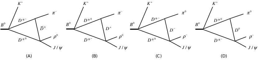
Figure 1: Triangle mechanisms (A,B) [(C,D)] for $B^{0}\to J/\psi\rho^{0}K^{+}\pi^{-}$ [$B^{0}\to J/\psi\rho^{-}K^{+}\pi^{0}$]. Triangle singularities from the diagrams (A,C,D) generate sharp peaks in $J/\psi\rho$ invariant mass ($M_{J/\psi\rho}$) distributions at $M_{J/\psi\rho}\sim 3.872,3.876$ and 3.875 GeV, respectively. In the text, the diagrams are referred to, from the left to right, as diagrams A, B, C, and D, respectively. Figures taken from Ref. sxn_x . Copyright (2020) APS.

$X(3872)$ belle_x3872_jpsi-rho is a prominent candidate of exotic hadrons, and its internal structure has been a controversial issue. The proposed ideas are such as a $D^{*0}\bar{D}^{0}$ molecule, diquark-antidiquark compact tetraquark, and an admixture the molecule with an excited charmonium. For getting closer to the correct understanding, a detailed analysis of various data relevant to $X(3872)$ would be important. In this context, an issue is whether a $X(3872)$ peak could be partly faked by a kinematical effect called the triangle singularity (TS). A triangle diagram like Fig. 1 may cause a TS at a classical-process-like condition where particles in the loop are all on-shell and they have collinear momenta with each other. The triangle amplitude for Fig. 1 is significantly enhanced by the TS, resulting in a bump in $J/\psi\rho$ and $J/\psi\rho\pi$ invariant mass distributions. The TS has been exploited to interpret spectrum bumps that may be due to $XYZ$ exotic hadrons ts_review ; ts_zc4430 ; ts_z4050 .

For $B^{0}\to J/\psi\rho^{0}K^{+}\pi^{-}$, the triangle diagram shown in Fig. 1(A)  meets the condition of a TS, and an $X(3872)$-like peak is expected in the $M_{J/\psi\rho^{0}}$ distribution ($M_{J/\psi\rho^{0}}$: $J/\psi\rho^{0}$ invariant mass) at $W\sim m_{D^{*-}}+m_{D^{*0}}$; $W$ is the $J/\psi\rho^{0}\pi^{-}$ invariant mass and $m_{x}$ refers to the mass of a particle $x$. The Belle experiment observed an $X(3872)$ peak in the $M_{J/\psi\pi^{+}\pi^{-}}$ distribution of $B^{0}\to(J/\psi\pi^{+}\pi^{-})K^{+}\pi^{-}$ belle_x3872kpi . In this work sxn_x , it is shown that TS from the diagram A creates an exactly $X(3872)$-like peak. Without adjusting any of the model parameters, this TS peak reproduces the experimentally measured $X(3872)$ mass of $\sim$0.01% precision and the tightly constrained width.

This finding means that we should take account of the TS contribution when extracting $X(3872)$ signal from $B^{0}\to J/\psi\rho^{0}K^{+}\pi^{-}$ or similar data in the TS region. According to a recent proposal guo_x3872 , the extracted $X(3872)$ signal accompanied by $X(3872)\pi$ and $X(3872)\gamma$ lineshapes can be analyzed to determine the $X(3872)$ mass. Because the non-resonant contribution from the diagram A is isospin conserving and not suppressed, an $X(3872)$-like contribution from this might be comparable to $X(3872)\to J/\psi\pi^{+}\pi^{-}$ which is suppressed by the isospin violation. For understanding the non-resonant mechanism and separating it from the $X(3872)$-pole contribution, we also study a charge analogous $B^{0}\to(J/\psi\pi^{0}\pi^{-})K^{+}\pi^{0}$ decay where triangle diagrams C and D create an $X^{-}(3876)$-like peak due to TS.

2 Model

The amplitude of the triangle diagram A for $B^{0}\to J/\psi\rho^{0}K^{+}\pi^{-}$ is given by

$$T = \int d\bm{q}\,\ {v_{J/\psi\rho^{0};D^{*0}\bar{D}^{0}}\,\ \over W-E_{D^{*0}}-E_{\bar{D}^{0}}-E_{\pi^{-}}}\Gamma_{\bar{D}^{0}\pi^{-},D^{*-}}{V_{K^{+}D^{*-}D^{*0},B^{0}}\over W-E_{D^{*-}}-E_{D^{*0}}}\,,$$ (1)

where $\bm{q}$ is a loop momentum. The energy of a particle $x$ is $E_{x}$ which depends on the particle mass ($m_{x}$), momentum ($\bm{p}_{x}$) and decay width ($\Gamma_{x}$) as $E_{x}=\sqrt{\bm{p}^{2}_{x}+m^{2}_{x}}-i\Gamma_{x}/2$; $\Gamma_{x}$ is nonzero for $D^{*}$. Similar amplitudes are given for triangle diagrams B, C, and D. The $B^{0}\to J/\psi\rho^{0}K^{+}\pi^{-}$ ($B^{0}\to J/\psi\rho^{-}K^{+}\pi^{0}$) decay amplitude includes the triangle mechanisms A and B (C and D) as a coherent sum. Due to the charge-parity invariance and isospin symmetry of the strong interaction, the triangle mechanisms A and B (C and D) exactly cancel each other if the mass and width are the same for the charged and neutral $D^{(*)}$ mesons. In the realistic situation, the TS peaks are hardly canceled while other contributions outside the TS region are significantly canceled.

The triangle diagrams A, C, and D cause TSs while the diagram B does not. This difference is caused by the fact that $D^{*0}\to D^{+}\pi^{-}$ at on-shell is forbidden and therefore the diagram B does not meet the kinematical condition for TS. Thus, in order to discuss TS from these triangle diagrams, it is essentially important to take account of mass differences between the isospin partners such as $({\pi^{\pm}},{\pi^{0}})$, $({D^{+}},{D^{0}})$, and $({D^{*+}},{D^{*0}})$. In the zero-width limit, the TSs occur from the triangle amplitudes for the diagrams A, C, and D in the kinematical region of $0<M_{J/\psi\rho}-(m_{a}+m_{b})\leq 0.2~{}{\rm MeV}$ and $0<W-(m_{D^{*-}}+m_{D^{*0}})\ \raise 1.29167pt\hbox{$<$\kern-7.5pt\lower 4.30554pt\hbox{$\sim$}}\ 1.0~{}{\rm MeV}$; $\{a,b\}=\{D^{*0},\bar{D}^{0}$}, {$D^{*0},D^{-}$}, and {$D^{*-},D^{0}$} for the diagrams A, C, and D, respectively. While TSs can be relaxed by finite widths in general, here the $D^{*-}$ and $D^{*0}$ widths are very small. Thus a very sharp TS peak is expected from the diagram A at $M_{J/\psi\pi^{+}\pi^{-}}\sim m_{D^{*0}}+m_{D^{0}}=3871.7$ MeV that looks very similar to $X(3872)$. We also expect that the diagrams C and D are coherently summed to give a sharp $X^{-}(3876)$-like peak in the $M_{J/\psi\pi^{0}\pi^{-}}$ distribution.

The $D^{*\pm}$ decay width has been measured to be $\Gamma_{D^{*\pm}}=83.4\pm 1.8$ keV pdg . Meanwhile, only an upper limit is known for the $D^{*0}$ decay width: $\Gamma_{D^{*0}}<2.1$ MeV pdg . $\Gamma_{D^{*0}}$ can be also calculated by assuming the isospin symmetry between $D^{*+}\to D^{+}\pi^{0}$ and $D^{*0}\to D^{0}\pi^{0}$, and also utilizing the branching ratio of $D^{*0}\to D^{0}\gamma$ measured experimentally. This gives $\Gamma_{D^{*0}}=55$ keV which will be adopted in our calculations.

Regarding the interaction vertices included in Eq. (1), $v_{J/\psi\rho^{0};D^{*0}\bar{D}^{0}}$ is an $s$-wave $D^{*0}\bar{D}^{0}\to J/\psi\rho^{0}$ interaction from which a $J/\psi\rho^{0}$ pair comes out with the spin-parity $J^{P}=1^{+}$, the spin-parity of $X(3872)$. An $X(3872)$-pole contribution is not included in $v_{J/\psi\rho^{0};D^{*0}\bar{D}^{0}}$. The vertex denoted by $\Gamma_{\bar{D}^{0}\pi^{-},D^{*-}}$ is for $D^{*-}\to\bar{D}^{0}\pi^{-}$. The $B^{0}\to D^{*-}D^{*0}K^{+}$ initial decay is described by $V_{K^{+}D^{*-}D^{*0},B^{0}}$. While $V_{K^{+}D^{*-}D^{*0},B^{0}}$ has a $W$-dependence, experimental information is not available. Because other processes such as $e^{+}e^{-}\to J/\psi D^{*}\bar{D}^{*}$ show significant enhancements near the $D^{*}\bar{D}^{*}$ threshold, we assume that $V_{K^{+}D^{*-}D^{*0},B^{0}}$ has a similar $W$-dependence. Each of the vertices include a dipole form factor on the momentum with a cutoff $\Lambda$; $\Lambda=1$ GeV is used unless otherwise stated. Following a standard procedure as detailed in Appendix B of Ref. 3pi , we calculate the double differential decay width $d\Gamma_{B\to J/\psi\rho^{0}K\pi}/dWdM_{J/\psi\rho}$ with the decay amplitude of Eq. (1). We then take account of the $\rho^{0}\to\pi^{+}\pi^{-}$ decay, giving $d\Gamma_{B^{0}\to J/\psi\pi^{+}\pi^{-}K^{+}\pi^{-}}/dWdM_{J/\psi\pi^{+}\pi^{-}}$.

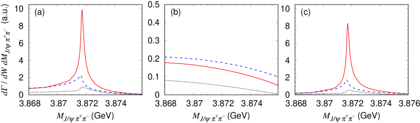
Figure 2: $J/\psi\pi^{+}\pi^{-}$ invariant mass ($M_{J/\psi\pi^{+}\pi^{-}}$) distributions for $B^{0}\to J/\psi\pi^{+}\pi^{-}K^{+}\pi^{-}$ given by the triangle diagrams of Figs. 1(A) and 1(B). $M_{J/\psi\pi^{+}\pi^{-}}$ is from $J/\psi$ and $\pi^{+}\pi^{-}$ from $\rho^{0}$ decay. The spectra at $W-(m_{D^{*0}}+m_{D^{*-}})=-1.0$, 0.0, and 1.2 MeV are shown by the black dotted, red solid, and blue dashed curves, respectively; $W$ denotes the invariant mass of the final $J/\psi\pi^{+}\pi^{-}\pi^{-}$ subsystem and $m_{D^{*0}}+m_{D^{*-}}=4017.1$ MeV. The panels (a) and (b) show the spectra from the triangle diagrams of Figs. 1(A) and 1(B), respectively; the panel (c) shows their coherent sum. Although the overall normalization of the figures is arbitrary, the relative heights among the curves in all the figures are a prediction of the model. Figures taken from Ref. sxn_x . Copyright (2020) APS.

3 Results

The double differential decay width $d\Gamma_{B^{0}\to J/\psi\pi^{+}\pi^{-}K^{+}\pi^{-}}/dWdM_{J/\psi\pi^{+}\pi^{-}}$ are shown as a function of $M_{J/\psi\pi^{+}\pi^{-}}$ in Figs. 2(a), 2(b), and 2(c) for the triangle diagrams A, B, and A+B, respectively. These spectra are for the TS region ($W\sim m_{D^{*0}}+m_{D^{*-}}$) and around. We find the outstanding peak created by the TS from the diagram A at $M_{J/\psi\pi^{+}\pi^{-}}\sim 3871.7$ MeV. The peak position seems exactly the precisely measured $X(3872)$ mass: $3871.69\pm 0.17$ MeV pdg . This peak position and the narrow width is a parameter-free prediction from the triangle diagrams A. We examined the cutoff dependence over $\Lambda=0.5-2$ GeV, and confirmed the stability of the position and shape of the TS peak. The other arbitrary parameters change the overall normalization only. The TS peak is such stable because: (i) the $D^{*}$ width is tiny and thus the TS is very close to the physical region and thus a dominant effect; (ii) details of the dynamics play little role for the TS. Figure 2 also shows that the TS peak height changes sensitively to $W$ because the TS occurs in the small $W$ window as discussed above.

Figure 2(b) shows that the triangle diagram B generates smooth lineshapes at $W\sim m_{D^{*0}}+m_{D^{*-}}$. The diagrams A and B look similar but they behave very differently. This difference is due to the fact that only the diagram A meets the TS condition. The tiny $D^{*}$ width is also a reason for this high selectivity of the TS condition. After taking the coherent sum of the diagrams A and B, as shown in Fig. 2(c), the diagram B cancel the smooth background-like contribution from the diagram A.

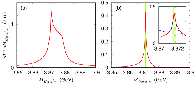
Figure 3: $M_{J/\psi\pi^{+}\pi^{-}}$ distributions given by the coherently summed triangle diagrams of Figs. 1(A) and 1(B). (a) The red solid curve is obtained by integrating the spectra in Fig. 2(c) and those in higher $W$ region with respect to $W$ over the whole $W$-region. (b) The red solid curve is obtained by the $W$-integral in the range of $-3~{}{\rm MeV}\leq W-(m_{D^{*-}}+m_{D^{*0}})\leq 4~{}{\rm MeV}$. The peak region is shown in the insert. The blue dashed curve shows the Breit-Wigner plus a background fitted to the red solid curve. The $X(3872)$ mass range from the PDG pdg is indicated by the green bands. Figures taken from Ref. sxn_x . Copyright (2020) APS.

The Belle data for $B^{0}\to J/\psi\pi^{+}\pi^{-}K^{+}\pi^{-}$ belle_x3872kpi shows a peak at $M_{J/\psi\pi^{+}\pi^{-}}\sim 3.872$ GeV in $d\Gamma_{B^{0}\to J/\psi\pi^{+}\pi^{-}K^{+}\pi^{-}}/dM_{J/\psi\pi^{+}\pi^{-}}$. This data includes the whole $W$ region allowed kinematically. We calculate a theoretical counterpart by integrating the spectra in Fig. 2(c) and also those in higher $W$ region with respect to $W$. Figure 3(a) is the obtained spectrum. While a sharp peak remains at $M_{J/\psi\pi^{+}\pi^{-}}\sim 3.872$ GeV, there is also a large shoulder near the $D^{*-}D^{+}$ threshold. This shoulder is from the threshold cusp generated by the diagram B. This spectrum is smeared with the experimental resolution and compared with the Belle data. The lineshape is found to be too broad to explain the data. Although this lineshape depends on the $W$-dependence assumed for the $B^{0}\to D^{*-}D^{*0}K^{+}$ vertex, the diagrams A and B does not seem likely to explain the Belle data.

Now the $W$-integral is limited to the TS region and around: $-3~{}{\rm MeV}\leq W-(m_{D^{*-}}+m_{D^{*0}})\leq 4~{}{\rm MeV}$. The resulting spectrum is given by the red solid curve in Fig. 3(b). A single narrow peak clearly appears. To quantify the peak position and width, we fit the spectrum with the common resonance($X$)-excitation mechanism, $B\to XK\pi$ and $X\to J/\psi\rho^{0}$. The fit gives the Breit-Wigner mass and width for $X$. A coherent background is also added with an adjustable quadratic polynomial of $M_{J/\psi\pi^{+}\pi^{-}}$. The fit result is given by the blue dashed curve in the small insert of Fig. 3(b). The fit does not work well in the tail region because: (i) the Breit-Wigner form and the spectrum shape are rather different; (ii) the background rapidly decrease near the higher end of the $M_{J/\psi\pi^{+}\pi^{-}}$ distribution due to the available phase-space. Nevertheless, the obtained Breit-Wigner mass and width still quantify the peak, and are $m_{\rm BW}=3871.68\pm 0.00$ MeV and $\Gamma_{\rm BW}=0.42\pm 0.01$ MeV, respectively; the ranges of the values are from the cutoff dependence. The Breit-Wigner mass value is larger than the $D^{*0}\bar{D}^{0}$ threshold by only a few keV. The Breit-Wigner parameters can be compared with the PDG value for $X(3872)$: $m_{\rm PDG}=3871.69\pm 0.17$ MeV and $\Gamma_{\rm PDG}<1.2$ MeV. These Breit-Wigner parameters have a very small cutoff dependence, and agree very well with the precise experimental measurement for $X(3872)$. From the above results, it is indicated that the TS peak from the diagram A might partly fake the $X(3872)$ signal in $B^{0}\to J/\psi\pi^{+}\pi^{-}K^{+}\pi^{-}$ at $W\sim m_{D^{*-}}+m_{D^{*0}}$. Thus, when applying the $X(3872)$ mass determination method of Ref. guo_x3872 to data, one needs to consider a possible contribution from the non-$X$ triangle mechanisms.

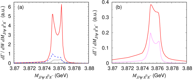
Figure 4: $M_{J/\psi\pi^{0}\pi^{-}}$ distributions for $B^{0}\to J/\psi\pi^{0}\pi^{-}K^{+}\pi^{0}$. The triangle diagrams of Figs. 1(C) and 1(D) are coherently summed to generate the spectra. $M_{J/\psi\pi^{0}\pi^{-}}$ is from $J/\psi$ paired with $\pi^{0}\pi^{-}$ from $\rho^{-}$ decay. (a) $M_{J/\psi\pi^{0}\pi^{-}}$ distributions for $W-(m_{D^{*0}}+m_{D^{*-}})=-1.0$, 0.0, and 1.2 MeV are shown by the black dotted, red solid, and blue dashed curves, respectively. (b) The spectra in the panel (a) are integrated with respect to $W$ to give the red solid curve. The integral in the limited region of $-3~{}{\rm MeV}\leq W-(m_{D^{*-}}+m_{D^{*0}})\leq 4~{}{\rm MeV}$ gives the magenta dotted curve. The overall normalization of the curves in the panel (a) is the same as those in Fig. 2. Figures taken from Ref. sxn_x . Copyright (2020) APS.

A charge analogous process, $B^{0}\to(J/\psi\pi^{0}\pi^{-})K^{+}\pi^{0}$, from the triangle diagrams C and D in Fig. 1 is now considered. Around the TS region ($W\sim m_{D^{*-}}+m_{D^{*0}}$), the triangle mechanisms generate the $M_{J/\psi\pi^{0}\pi^{-}}$ distribution as in Fig. 4(a). Each of the triangle diagrams C and D hits a TS to generate a sharp peak. Their coherent sum appears as the clear twin peaks in the figure. We see again the acute $W$ dependence of the spectra. We integrate the spectra in Fig. 4(a) and those in higher $W$ region with respect to $W$, the red solid curve in Fig. 4(b) is obtained. When we limit the $W$-integral near the TS region only, the magenta dotted curve is obtained. We find the clear peak after the $W$-integral. A future experiment could find this $X^{-}(3876)$-like peak. If the peak is observed experimentally, this would be a clear identification of TS in data because no charged and very narrow resonance is known in this energy region.

The non-resonant $X(3872)$-like peak is generated by the diagram A in the TS region. When $X(3872)$ signal is analyzed by the method of Ref. guo_x3872 to determine the $X(3872)$ mass, this TS contribution has to be eliminated in advance. We proposed a method to estimate the non-resonant contribution by studying the charge analogous process. Details are discussed in Ref. sxn_x .

References

- (1) S.K. Choi et al. (Belle Collaboration), Phys. Rev. Lett. 91, 262001 (2003).
- (2) F.-K. Guo, X.-H. Liu, and S. Sakai, Prog. Part. Nucl. Phys. 112, 103757 (2020).
- (3) S.X. Nakamura and K. Tsushima, Phys. Rev. D 100, 051502(R) (2019).
- (4) S.X. Nakamura, Phys. Rev. D 100, 011504(R) (2019).
- (5) A. Bala et al. (Belle Collaboration), Phys. Rev. D 91, 051101(R) (2015).
- (6) S.X. Nakamura, Phys. Rev. D 102, 074004 (2020).
- (7) F.-K. Guo, Phys. Rev. Lett. 122, 202002 (2019).
- (8) M. Tanabashi et al. (Particle Data Group), Phys. Rev. D 98, 030001 (2018).
- (9) H. Kamano, S.X. Nakamura, T.-S.H. Lee, and T. Sato, Phys. Rev. D 84, 114019 (2011).