A search for variable subdwarf B stars in TESS Full Frame Images
II. Variable objects in the northern ecliptic hemisphere

Abstract

We report the results of our search for pulsating subdwarf B stars in Full Frame Images collected during Year 2 of the TESS mission and covering the northern ecliptic hemisphere. This is a continuation of our effort we presented in Paper I. We found 13 likely new pulsating subdwarf B stars, 10 pulsating candidates that are identified as other hot subdwarfs, and 30 spectroscopically unclassified objects that show amplitude spectra typical of pulsating subdwarf B stars. We found 506 variable objects, most of them spectroscopically unclassified, hence their specific variability class yet to be confirmed. Eclipsing binaries with sharp eclipses sample comprises 33 systems. For 12 of them we derived precise orbital periods and checked their stabilities. We identified one known and five new candidate HW Vir systems. The amplitude spectra of the 13 likely sdB pulsators are not rich in modes, hence any further analysis is not possible. However, we selected three candidates for pulsating subdwarf B stars that show the richest amplitude spectra and we performed a mode identification deriving modal degrees of most of the detected modes. In total, in both ecliptic hemispheres, we found 15 likely pulsating pulsating subdwarf B stars, additional 10 candidates for pulsating subdwarf B stars, 66 other variable subdwarf B stars, 2076 spectroscopically unconfirmed variable stars, and 123 variable non-sdB stars.

1 Introduction

Sahoo et al. (2020, hereafter: Paper I) reported their findings in the southern ecliptic hemisphere f 1807 variable stars, including two likely new pulsating subdwarf B stars (sdBV), 26 non-pulsating sdBs, and 83 spectroscopically unclassified objects whose amplitude spectra show peaks in the sdBV g-mode region. The bulk of the variables have no spectral classification so the result of Sahoo et al. (2020) defines a catalog of objects that require spectroscopic verification.

We continued our effort to search for variable subdwarf B stars (sdB) in the northern ecliptic hemisphere observed by TESS and stored in Full Frame Images (FFI). Our main goal is to complete the census of variable sdBs in the TESS field-of-view. Many targets have been incorporated in the short cadence, either 2 min or 20 sec, monitoring, however this observing mode is limited in number of targets and therefore not all sdBV candidates will be observed. Our search is not subject to any pre-approval since we use FFI images that are stored automatically and all targets in those images are available for data processing. Handling all objects detectable in the FFIs, although desirable, is technically difficult (processing would take months if not years), hence we focus on targets listed in the sdB catalogue described by Geier (2020).

Subdwarf B (sdB) stars are identified as objects located at the blue end of the horizontal branch, often called the extreme horizontal branch (EHB), in the Hertzsprung-Russell diagram (Heber, 2016). These stars are compact in size, with surface gravities, $\log$ (g/ $\mbox{cm}\,\mbox{s}^{-2}$), of 5.0 to 5.8, which translates into radii of 0.15 – 0.35 R_☉. SdBs are blue due to their high effective surface temperature (T_eff) ranging between 20,000 and 40,000 K. The sdB stars have masses 0.47 M_☉ on average, which is sometimes called the canonical mass (Heber, 2016).

Pulsations in sdBs were discovered observationally by Kilkenny et al. (1997) and theoretically by Charpinet et al. (1997). The pulsations were found at both low and high frequencies. The low frequencies (long periods of hours) are explained by gravity modes, while the high frequencies (short periods of minutes) are explained by pressure modes (Fontaine et al., 2003). To increase a sample of known pulsating sdB (sdBV) stars, it was essential to make an effort at more discoveries. First discoveries were made from the ground and detections were limited to sdBVs showing pressure modes. They were easier to detect because of their higher observable amplitudes and shorter periods as compared to sdBVs showing gravity modes. Only a handful of sdBVs were found to be pulsating in both types of modes, with Balloon 090100001 being the best example (Baran et al., 2009). To date, there are around 130 sdBV found in both ground and Kepler space data (Holdsworth et al., 2017; Reed et al., 2018). Additional 200+ sdBVs are detected in TESS short cadence data and the full list will be reported elsewhere.

SdBVs are found in both open (Reed et al., 2012) and globular (Randall et al., 2009) clusters but mostly in the Galactic field. We still lack a complete all-sky search for sdBVs, which prevents a comprehensive analysis of pulsation properties correlated with stellar population to conclude the location of instability strip(s) or physical parameters (especially masses). An all-sky search for sdBVs, along with Gaia parallaxes would tell us about the distribution of these stars in the Galaxy and contribute toward pulsation-stellar population relationships.

We aimed at selecting sdBs and sdB candidates that were not included in the predefined target list, producing time-series data directly from FFIs and making mode identifications of the most suitable cases showing pulsations. The results we present here are based on data collected during Year 2 in Sectors 14–26. Each sector is monitored for about 27 days. In Section 2 we describe the source of our targets, the selection process and data processing. In Section 3 we present objects with found variables. Section 4 reports our mode identification effort, followed by Section 6 that summarizes our results.

2 Target selection and data processing

To select sdB candidates we used the sdB database reported by Geier (2020), which was prepared based on ESA Gaia Data Release 2 (DR2) and several ground-based multi-band photometry surveys. Geier (2020) used color indices, absolute magnitudes and reduced proper motions to select the most suitable sdB candidates. The database is limited to Gaia G mag = 19 and contains 39 800 objects. From this sample we selected 15 191 objects located in the northern ecliptic hemisphere and the TESS field of view. Using Gaia IDs and target coordinates we applied TOPCAT (Taylor, 2005) and rejected 548 targets that were assigned to be observed in the short cadence mode. Then, we used Tesscut (Brasseur et al., 2019) to collect sector information targets in our sample that will be observed in, and targets with no sector assignment were also rejected. Finally, we filtered targets observed in sectors 14-26 and we ended up with 5 816 targets. It turned out that 464 targets have no useful data, so these were also rejected from our sample, hence the final number of targets was 4 804. For completeness, we have included targets with non-sdB spectral classification as it may happen that some of these already classified objects will be reclassified as sdBs with further analysis. In addition, even if the stars will not be reclassified as sdBs, other researchers may find it useful to have these objects identified as variables.

The extraction process is exactly the same as described by Sahoo et al. (2020). First, we used the Eleanor (Feinstein et al., 2019) for downloading and processing data directly from TESS FFIs, which we downloaded from the "Barbara A. Mikulski Archive for Space Telescopes" (MAST). We specified a square target mask of 15 pixels on side and a square background mask of 31 pixels on side. Eleanor delivers raw and corrected time-series data. The raw data is a sky-subtracted simple aperture photometry, which is basically a sum of all flux within an optimal aperture for each timestamp. The corrected data account for known satellite artifacts. We extracted both data sets and have chosen the one that shows better signal-to-noise (S/N).

Then, we used lightkurve python package (Lightkurve Collaboration et al., 2018) to detrend and remove outliers from time-series data. Finally, we normalized fluxes by calculating (f/$\bar{\rm f}-$1)$\cdot$1000, where f and $\bar{\rm f}$ stands for a flux and median flux respectively, reporting amplitudes in parts per thousand (ppt). We remind the reader that the Eleanor does not account for a crowding metric correction and a flux fraction, which often results in an overestimated average flux and a diluted amplitude of a flux variation. Therefore, the amplitudes are often not realistic. In case of sdBV stars, the amplitudes are not so important, but they are for accurate modelling of eclipsing binaries or classical pulsators.

We searched for a flux variation in amplitude spectra we calculated for each target. We used a threshold of S/N ratio of 4.5 (Baran et al., 2015). The cadence of 30 min defines the Nyquist frequency at 277 ${\mu}$Hz (24 c/d). This limits our search to gravity mode sdBVs only.

3 The zoo of our findings

We detected significant flux variations in 506 objects, including 53 sdBs, 33 subdwarfs (sd), 374 not spectroscopically classified, and 46 classified as non-sdBs. To identify sdB objects we used the sdB database (Geier, 2020) and the Simbad database (Wenger et al., 2000). We listed all variable objects in Tables 1–6, including those in on-line material, which provide basic information on our findings and possible contamination. The large square pixels, 21 arcsec on side, cause serious issues in crowded regions of the sky as an optimal aperture, typically 2–3 pixels, may contain neighboring objects. In case the optimal aperture covers neighboring sources, and we are not positive about which object shows a flux variation, we made remarks according to the following rule. If an optimal aperture contains more than five objects we marked it as crowded region, if the optimal aperture is densely covered by stars, e.g. a cluster region, we marked it as very crowded region, if a few objects (< 5) were spotted, we specified the number of objects within a given radius. In case of just one neighboring object within an optimal aperture, we provided the distance to the object, and we provided its designation, if any. If we found that any of our targets is already known as a variable star, we provided a reference. Even though these targets are not new variables, we included them for completeness.

3.1 Spectroscopically confirmed sdB variables

We found 53 variable objects classified as sdBs and we list them in Table 1. This table is divided into three groups. The first group contains 13 objects with peaks above 60 $\mathrm{\mu}$Hz and we identified them as likely pulsating sdBs. Our interpretation may not be correct, since binary peaks can also be detected above 60 $\mathrm{\mu}$Hz and that is why we call this group "likely sdBV stars", as better quality data must confirm our interpretation. We show the amplitude spectra of these objects in Figure 1. All these objects show poor g-mode spectra and further analysis related to pulsations in sdBs cannot be performed. The second group contains 15 sdBs that show clear orbital flux variation and do not show any pulsation signature. We found four eclipsing binaries with sharp eclipses, four objects showing one maximum, which can be interpreted as e.g. a reflection effect, five objects showing two maxima, which can be either eclipsing and/or ellipsoidal systems, and two systems showing one asymmetric maximum that is typical of classical pulsators. We show the phased time-series data in Figure 2. Gaia DR2 4467130720760209152 shows HW Vir flux variations, while Gaia DR2 880252005422941440 was, the most likely, mistakenly classified as RR Lyrae star by Drake et al. (2014). The optimal aperture for Gaia DR2 382086995098288896 overlaps with Gaia DR2 382086995093288256, which has been reported as variable by Drake et al. (2014). The period we find is half the one cited by Drake et al. (2014) and most likely the variation we find comes from the latter object. The third group contains 25 sdBs that show flux variations that cannot be pulsations, while the phased time-series data either do not show significant variation or multiple peaks that make the phased time-series looks messy. We plot the amplitude spectra in Figure 3. Most of the time they show related peaks likely indicating a binary nature of the systems, while single peaks below 60 $\mathrm{\mu}$Hz are atypical for sdBVs. Gaia DR2 2129739699292289152 is found to be variable by Østensen et al. (2011).

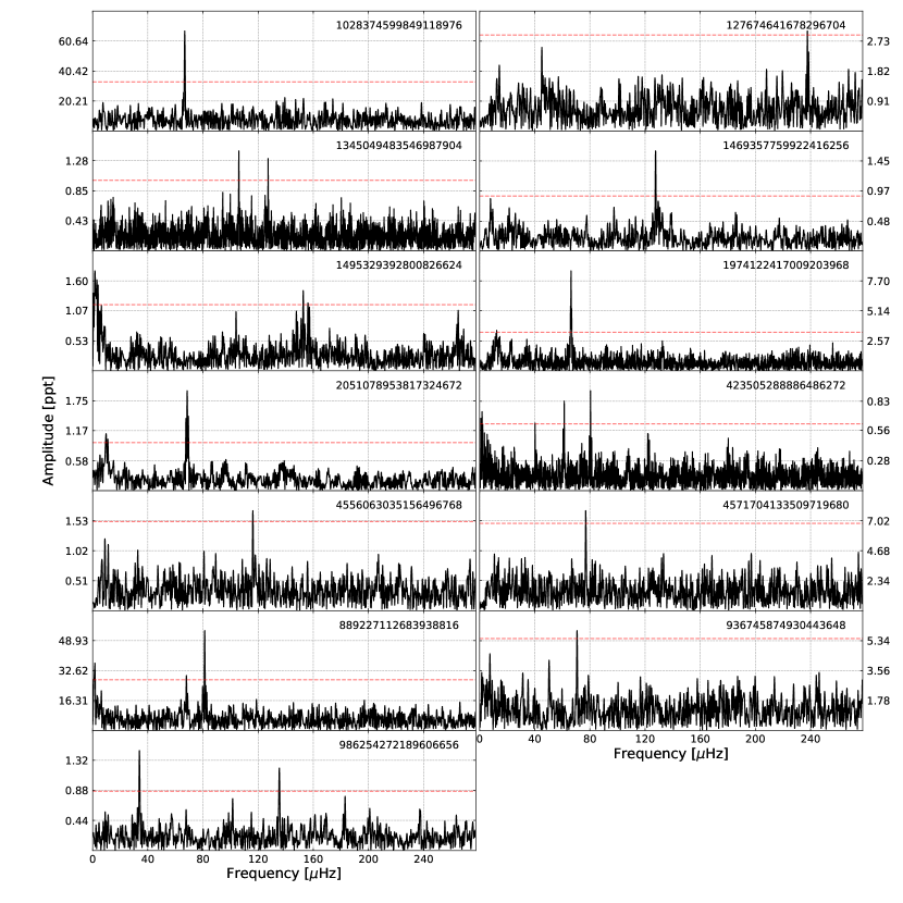
Figure 1: Amplitude spectra of 13 sdBV stars listed in the first group of Table 1. Horizontal red dashed lines indicate S/N = 4.5 detection threshold (all relevant figures). The long numbers in all figures denote Gaia DR2 numbers of specific stars.

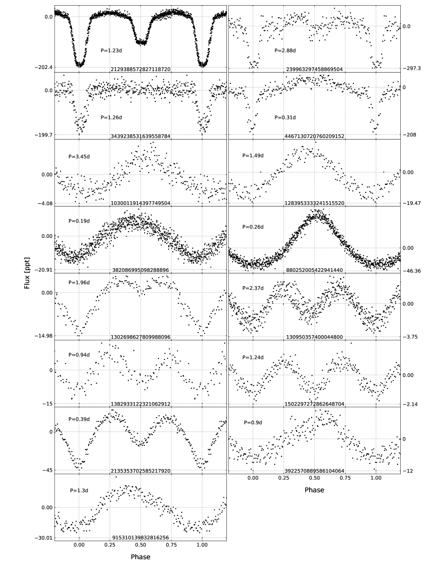
Figure 2: Phased and binned time-series data of variable sdB stars listed in the second group of Table 1.

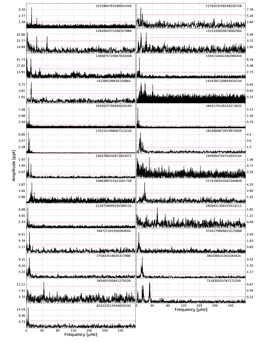
Figure 3: Amplitude spectra of variable sdB stars listed in the third group of Table 1.

Table 1: Basic information of 53 objects classified as sdBs. Time-series data or amplitude spectra of these objects are plotted in Figures 1, 2 and 3. Objects in all tables and figures are sorted by Gaia ID, not accounting for the length of the numbers.

			G		Period
Gaia DR2	TIC	Name	[mag]	Sector	[days]	Remarks
sdBVs – Figure 1
1028374599849118976	802232206	SDSS J082428.41+512601.6	18.7153	20	0.1734	-
127674641678296704	353892824	KUV 02281+2730	15.1482	18	0.0487	-
1345049483546987904	159850392	GALEX J17566+4125	14.2792	25,26	0.08 - 0.13	-
1469357759922416256	321423000	SDSS J132432.37+320420.9	16.6387	23	0.0907	-
1495329392800826624	23746001	PG 1350+372	14.3133	23	0.06 - 0.09	-
1974122417009203968	305867900	LAMOST J213911.57+453915.2	16.5692	15,16	0.1745	4 objects within 21"
2051078953817324672	122366140	SDSS J192059.78+372220.0	15.7712	14	0.1689	4 objects within 21"
423505288886486272	445380420	LAMOST J005821.83+553750.9	13.2004	17,18	0.12 - 0.35	2 bright objects within 21"
4556063035156496768	363766470	HS 1741+2133	14.0105	26	0.0996	object 7" away
4571704133509719680	1309303943	SDSS J170256.38+241757.9	19.0562	25	0.1504	5 objects within 21"
889227112683938816	741122759	LAMOST J065538.32+312339.8	17.0121	20	0.1 - 0.2	-
936745874930443648	741726760	SDSS J075937.15+541022.2	17.7817	20	0.1638	object 14" away
986254272189606656	742806233	LAMOST J073935.74+564233.2	16.6757	20	0.08 - 0.4	-
variable sdBs – Figure 2
2129388572827118720	1882909457	Kepler J19211+4759	17.6946	14,15	1.2319	-
239963297458869504	642677463	SDSS J030749.25+411401.6	17.6208	18	2.8795	-
3439238531639558784	172171754	KUV 06290+3235	16.2259	20	1.2607	-
4467130720760209152	356085716	PG 1628+181	15.3912	25	0.3094	HW Vir
1030011914397749504	802252743	SDSS J084556.15+542357.6	18.8719	20	3.4529	bright object 32" away
1283953333241515520	156692388	SDSS J142559.17+284715.2	16.7380	23	1.4896	2 objects within 30"
						Gaia DR2 382086995098288256
382086995098288896	440171028	FBS 0021+418	15.7920	17	0.1935	Drake et al. (2014) 12" away
880252005422941440	4161582	LAMOST J073756.25+311646.5	13.5824	20	0.2574	RR Lyr, Drake et al. (2014)
1302698627809988096	459285617	PG 1610+239A	13.0425	24,25	1.9579	-
130950357400044800	620408944	KUV 02226+2835	17.3505	18	2.3714	4 bright objects within 53"
1382933122321062912	29385876	FBS 1554+403	14.0505	24	0.9382	-
1502297272862648704	393911299	BSD 33-110	11.3418	16,22,23	1.2393	-
2135353702585217920	27766711	KIC 12021724	15.4766	14,15	0.3879	-
3922570889586104064	86277081	PG 1206+165	13.6527	22	0.9000	-
915310139832816256	27319282	PG 0825+428	15.0510	20	1.2956	-
variable sdBs – Figure 3
1075984763296931456	313355841	PG 1155+741	15.3427	14,20,21	0.8691	-
1270423258548105728	357500534	PG 1517+265	15.8639	24	1.0576	-
1282064372266357888	1101440486	SDSS J145634.65+300450.9	16.7505	24	0.4367	-
1313140659676082560	298336617	PG 1648+315	15.8415	25	1.0069	-
1380875729907633408	1200857883	KUV 16160+4120	17.0611	24,25	1.0133	-
1394116942282089344	155947880	PG 1524+439	15.0667	23,24	1.5255	-
142389199635140864	68156854	FBS 0255+379	14.6431	18	0.9211	-
1434391159854454144	233683336	PG 1723+603	15.5060	14-17,19-26	0.25 - 2	-
1629425796564620160	198176924	HS 1615+6341	15.8057	14-26	1.7533	-
1644174130142213632	1102460173	GALEX J15134+6454	19.6992	14-16,21-23	3.3196	-
1702141998067113216	257002616	TYC 4559-2508-1	10.1276	14-15,20-22,26	2.1527	-
1816969872879974656	219647492	KPD 2022+2033	13.6885	14	1.13872	crowded field
1904789240973843072	128784655	FBS 2238+369	14.1718	16	1.9962	-
1949954704743455104	256785606	FBS 2155+374	14.1748	15,16	0.3534	3 objects within 21"
1966389723521001728	372181885	LAMOST J213853.04+402415.7	14.4891	15,16	0.8289	object 20" away
2114190543287369856	193944889	FBS 1801+431	14.3941	25	0.5566	-
2129739699292289152	26492416	Kepler J192652+490849	15.3157	14,15	3.0976	Østensen et al. (2011)
2809421366255514112	301799840	PG 0033+266	14.2751	17	0.2180	-
346721341030064640	291885456	FBS 0156+439	15.3142	18	1.4519	4 objects within 21"
3744179869623125888	138173268	Balloon 81300002	13.8032	23	1.9374	-
375833419635317888	238627422	FBS 0048+432A	14.6036	17	1.4989	-
380338531092183424	288292938	LAMOST J002124.79+402857.1	15.5119	17	0.7905	crowded field
385493350841270528	440072535	FBS 0013+434	15.5555	17	0.2600	-
751830524767171200	450325981	CBS 129	11.2693	21	0.3 - 10	-
833223213044650240	406756832	PG 1022+459	15.8435	21	2.4213	-

3.2 Spectroscopically confirmed other subdwarf variables

We found 33 objects, which are classified by Geier (2020) as subdwarfs, showing flux variations similar to the objects reported in Section 3.1. These objects are not classified as sdBs but as sdO (14), sdOB (6), or just sd (13). The objects of the latter class require further classification to confirm the spectral type to O, B or OB. We list these objects in Table 2. It is separated into three groups in the same way as sdBs objects in Section 3.1. Most of the objects in the first group, i.e. likely pulsating sds, are single peaks, with Gaia DR2 1952553606634620928 being the richest among all sds and sdBs, having five peaks above our threshold of S/N = 4.5. We show the objects of this group in Figure 4. The first three objects in the second group (Figure 5) are eclipsing binaries, characterized by sharp eclipses, with Gaia DR2 1820963913284517504 showing an HW Vir shape of the phased time-series data, and having one of the longest orbital period among as compared to other HW Vir systems. The system was found to be planetary nebula, so the primary component is not an extreme horizontal branch star. Next two objects in Figure 5 show one symmetric maxima, the following object shows two maxima (eclipsing systems) and the two remaining ones show one asymmetric maxima. Gaia DR2 759081078102507264 has been previously found to be variable by Drake et al. (2014). The third group contains objects selected based on the same criteria as in Section 3.1. The majority of these are most likely binaries and we plot their amplitude spectra in Figure 6.

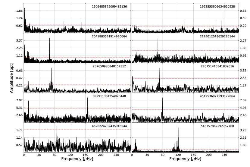
Figure 4: Amplitude spectra of 10 sd variable stars listed in the first group of Table 2.

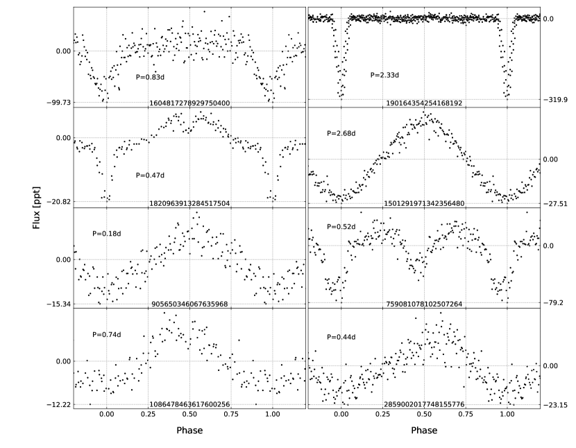
Figure 5: Phased and binned time-series data of variable sd stars listed in the second group of Table 2.

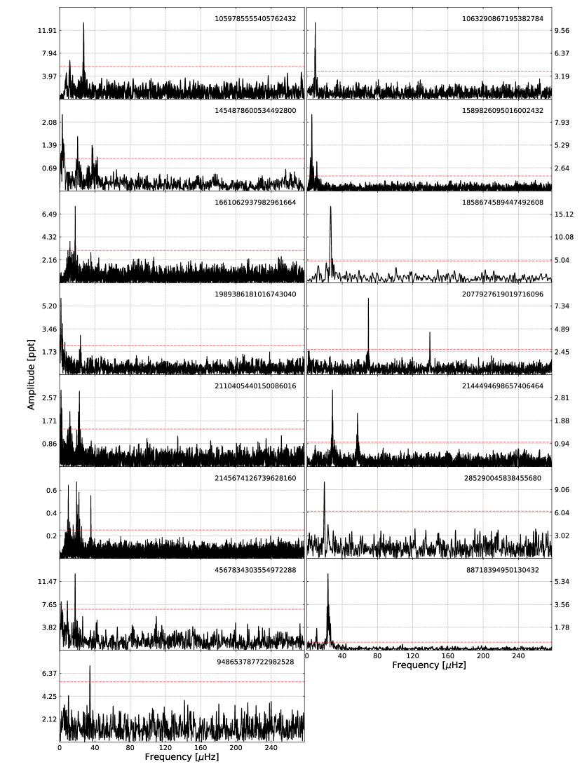
Figure 6: Amplitude spectra of variable sd stars listed in the third group of Table 2.

Table 2: Basic information of 33 objects classified as sds. Time-series data or amplitude spectra of these objects are plotted in Figs. 4,5 and 6.

			G		Period
Gaia DR2	TIC	Name	[mag]	Sector	[days]	Remarks
sdVs – Figure 4
1906485375099435136	259091223	FBS2209+354	14.3005	15,16	0.07-0.13	-
1952553606634620928	407657360	LAMOSTJ214600.31+372119.7	14.6625	15,16	0.045 - 0.1	4 objects within 32"
2041883531914920064	20688004	GALEXJ18578+3048	13.7315	14,26	0.1726	2 objects within 21"
2128012018629286144	1882679963	KeplerJ19352+4555	17.1559	14,15	0.1766	-
237650985848157312	194781979	LAMOSTJ032717.71+410344.5	10.1918	18	0.1594	-
276751410341839616	372463918	SDSSJ041536.69+560222.5	14.3548	19	0.1627	-
399911384254920448	354155298	SDSSJ012458.96+475640.9	16.9215	17,18	0.0701	2 objects within 32"
4512536977593172864	346754900	SDSSJ184336.23+183541.2	15.5500	26	0.1462	crowded field
4526224282435916544	1684677537	LAMOSTJ181102.81+173759.8	17.1021	26	0.1349	4 objects within 21"
546757862292757760	396013351	SDSSJ022718.01+733611.1	14.8957	18,19,25	0.09 - 0.2	3 objects within 21"
variable sds – Figure 5
1604817278929750400	1001259992	SDSSJ142017.21+513904.1	18.9939	16,22,23	0.8253	-
190164354254168192	426264139	LAMOSTJ054257.76+391151.2	14.9411	19	2.3316	3 objects within 21"
						Bond et al. (1978),
1820963913284517504	1842385646	PNA 6663	15.0966	14	0.4653	very crowded field
1501291971342356480	1001024276	SDSSJ133627.35+422910.90	18.5819	22,23	2.6765	object 24" away
905650346067635968	139150535	SDSSJ080327.93+342140.7	15.0617	20	0.1824	object 19" away
759081078102507264	144353046	FBS1125+345	16.1367	22	0.5228	Drake et al. (2014)
1086478463617600256	85210423	GALEXJ07354+6132	13.9744	20	0.7398	-
2859002017748155776	58105203	PG0023+298	15.0708	17	0.4415	-
variable sds – Figure 6
1059785555405762432	103802941	PG1030+665	15.4705	14,21	0.4251	-
1063290867195382784	86374556	SDSSJ093654.17+621449.5	15.8320	20,21	1.2309	-
1454878600534492800	199497852	vZ1128	14.9662	23	0.5684	crowded field
1589826095016002432	116307277	PG1447+459	14.9342	16,23	2.0965	2 objects within 21"
1661062937982961664	1001364570	PG1348+606	16.3181	15,16,22	0.6538	-
1858674589447492608	230775376	Feige114	13.5045	15	0.4302	4 bright objects within 21"
1989386181016743040	252589558	KPD2259+5149	13.8445	16,17	0.4920	crowded field
2077927619019716096	271345879	KPD1938+4220	15.5654	14,15	0.1660	4 objects within 21"
2110405440150086016	157583405	SDSSJ183620.82+405938.5	14.5125	14,26	0.5 - 10	object 13" away
2144494698657406464	48191737	O11J185046+510738	13.6951	14,15,26	0.3990	-
2145674126739628160	47670365	O11J183634+531657	12.4810	14,15,19,22,25,26	0.31 - 2	2 objects within 21"
285290045838455680	668928634	SDSSJ045912.47+605156.6	18.7139	19	0.5851	-
4567834303554972288	471013471	PG1707+214	15.6066	25	1.3179	3 bright objects within 3
88718394950130432	426419494	SDSSJ024113.47+215743.2	12.7945	18	0.9694	-
948653787722982528	742179265	SDSSJ072401.73+410320.9	19.3820	20	0.3371	4 objects within 32"

3.3 Spectroscopically unconfirmed sdBV candidates

We found 30 objects that show multi-unrelated-peak amplitude spectra, which we interpret as pulsations. We show the amplitude spectra of these objects in Figure 7. The spectra show peaks in the g-mode region of sdBVs and that is why these objects are of particular interest to us. These stars may also be $\delta$ Scuti stars, though Geier (2020) applied a color index criterion to avoid cool stars, or $\beta$ Cep stars. Geier (2020) provides detailed arguments using Gaia color indices that these targets are hot subluminous stars and occupy the region -0.7 < G_BP-G${}_{\rm RP}\lesssim$ 0.7 in the Gaia colour space. These objects are not spectroscopically classified so we are unable to make any definite conclusion about their pulsation nature, however the amplitude spectra are richer in peaks that any of likely sdBVs or sdVs we show in Figures 1 and 4. We listed these objects along with their basic information in Table 3. Of special interest are Gaia DR2 2129988841754560000, Gaia DR2 438585365733719168 and Gaia DR2 537697439806045824 since their spectra are the richest, containing enough peaks to make a mode identification by means of period spacings. Even though we are not positive the three objects are sdBVs, our suggested mode assignment may be useful if a sdB classification is confirmed by future spectroscopic analyses. We present the result of the mode identification in Section 4. Gaia DR2 2126670309505084672 was found to be a variable by Reinhold et al. (2013) and denoted KIC 9020774. The optimal aperture for Gaia DR2 2127067508079685888 overlaps with Gaia DR2 2127067542439425536 (KIC 8879964) whose variability with the same period has been reported by Reinhold et al. (2013). It is most likely that the variability comes from the latter object.

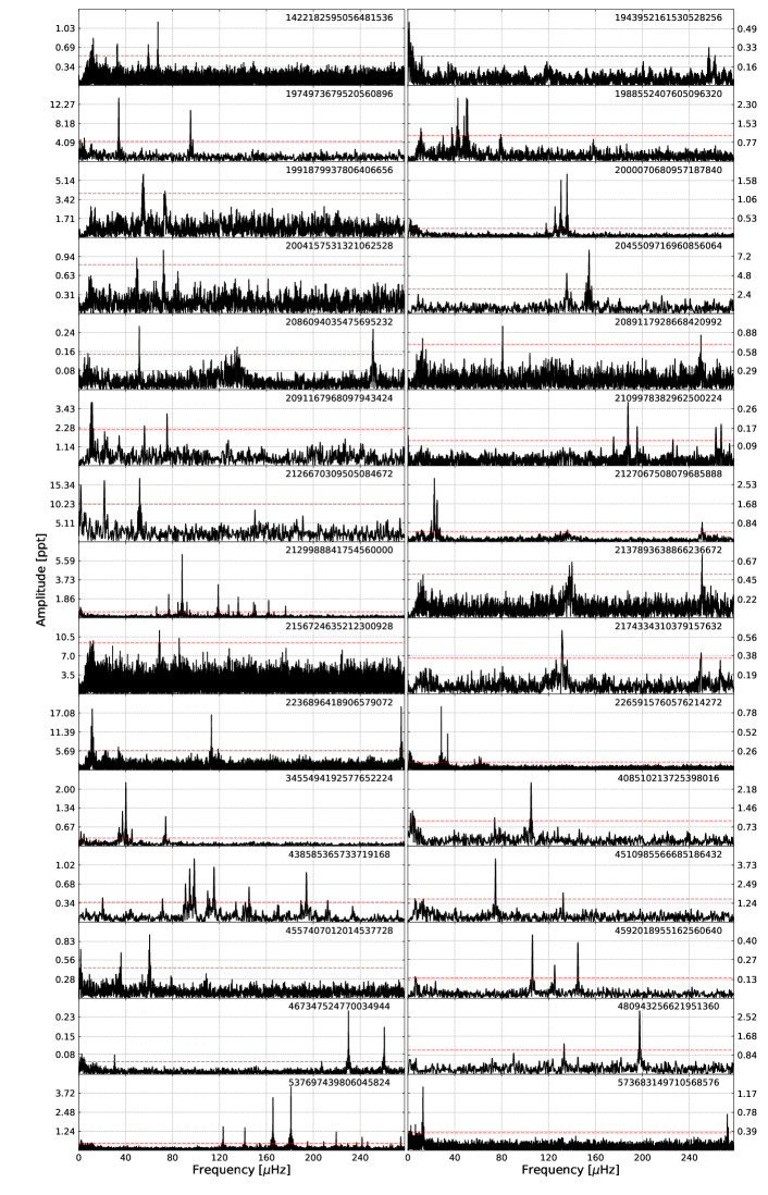
Figure 7: Amplitude spectra of sdBV candidates that are not spectroscopically classified listed in Table 3.

Table 3: Basic information of 30 sdBV candidates that are not spectroscopically classified. We show amplitude spectra of these objects in Figure 7

		G
Gaia DR2	TIC	[mag]	Sector	Remarks
1422182595056481536	320525680	13.8708	14-21,23-26	2 objects within 21"
1943952161530528256	431548978	15.6118	17,24	-
1974973679520560896	311792028	15.8844	16	4 objects within 21"
1988552407605096320	66784300	14.8772	16,17	5 bright objects within 21"
1991879937806406656	2044241813	18.4712	16,17	3 objects within 21"
2000070680957187840	2013748140	17.9850	16,17	crowded field
2004157531321062528	2014779767	17.4638	16,17	crowded field
2045509716960856064	1873643239	17.8928	14	2 bright objects within 21"
2086094035475695232	1881839953	17.9128	14,15	crowded field
2089117928668420992	364910983	16.2671	14,15,16	2 bright objects within 21"
2091167968097943424	1550027150	17.4874	26	3 objects within 21"
2109978382962500224	1550453189	17.2795	14,26	-
2126670309505084672	159722705	15.0028	15	Reinhold et al. (2013)
2127067508079685888	159108456	16.3927	14,15	KIC 8879964, Reinhold et al. (2013) 9" away
2129988841754560000	1882977987	16.5499	14,15	crowded field
2137893638866236672	1883445550	18.2584	14,15,16	-
2156724635212300928	233607898	16.0483	14-17,19-26	object 10" away
2174334310379157632	2017774400	16.2330	16,17	crowded field
2236896418906579072	236868718	17.3690	14-17,24	-
2265915760576214272	229786221	13.4680	14-17,19-23,25-26	-
3455494192577652224	116747928	11.4189	19	-
408510213725398016	623262377	18.6718	18	3 objects within 21"
438585365733719168	428055301	15.5791	18	crowded field
4510985566685186432	298514603	15.4720	26	crowded field
4557407012014537728	311431337	12.0714	25,26	-
4592018955162560640	24261156	16.0873	26	crowded field
467347524770034944	51026936	16.4141	18,19	5 bright objects within 32"
480943256621951360	328663453	16.0841	19	object 13" away
537697439806045824	407425099	16.4121	18,19,24,25	crowded field
573683149710568576	461640603	14.2553	18,20,25,26	2 bright objects within 21"

3.4 Spectroscopically unclassified variables

This sample includes all objects that are not spectroscopically classified and do not show amplitude spectra typical for sdBs.

We found 23 eclipsing binaries with sharp eclipses that are not yet spectroscopically classified. They all show distinct eclipses and are either detached or semi-detached binaries. We report the entire list of these objects in Table 4. Possible contact binaries are not included in this group. We separated these 23 objects into two groups. The first group consists of 16 objects that show only primary eclipses. This may be a consequence of a low inclination angle and/or small size of primary components with respect to the distance between them. We show phased time-series data of these objects in Figure 8. There are five candidates for HW Vir systems. They show no detectable secondary eclipses but they show a flux increase between primary eclipses that is characteristic of a reflection effect. None of these five objects has been reported thus far. The second group consists of seven objects that show both primary and secondary eclipses. We show phased time-series data of these objects in Figure 9. Gaia DR2 2126055476346353792 has been previously identified as a cataclysmic variable by Scaringi et al. (2012) and denoted KIC 7524178.

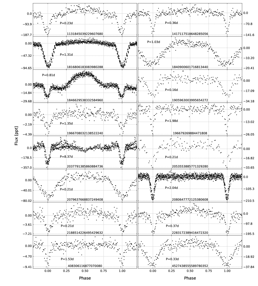
Figure 8: Phased time-series data of eclipsing binaries that show sharp primary eclipses only, and are listed in the first group of Table 4.

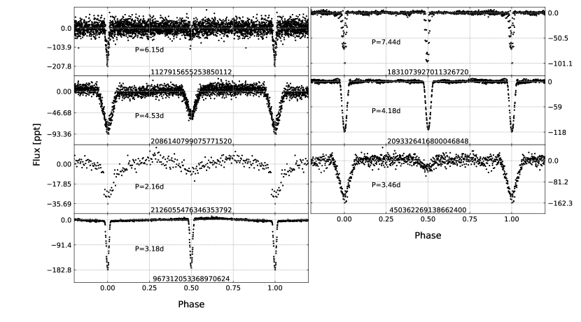
Figure 9: Phased time-series data of eclipsing binaries that show sharp both primary and secondary eclipses, and are listed in the second group of Table 4.

Table 4: Basic information of 23 spectroscopically unclassified eclipsing binaries. We show the time-series data of these objects in Figures 8 and 9.

		G		Period
Gaia DR2	TIC	[mag]	Sector	[days]	Remarks
Only primary eclipses detected – Figure 8
1131845039229607680	459182998	16.1614	14,26	0.2344	HW Vir candidate
1417117518648285056	1400704733	17.0325	14-15,17-18,20-21,23-26	0.3637	HW Vir candidate
1816806183083980288	1943324398	17.2206	14	1.3135	crowded field
1840900601716813440	1951174238	18.9249	15	1.0329	3 objects within 21"
1846629538332584960	15040115	11.8285	15	0.8099	3 objects within 32"
1905963003995654272	274852575	16.9924	16	0.1610	bright object 7" away
1966708032138522240	372019916	15.4010	15,16	1.3454	2 objects within 21"
196679269884471808	701334595	17.7576	19	1.9838	2 objects within 21"
2037791385860884736	1712396254	18.6493	14	8.3660	crowded field
2053553885771329280	137755255	15.4784	14	0.2060	3 objects within 21"
2079637668837249408	1881471898	17.4596	14,15	0.2075	4 objects within 21"
2080647772125380608	1881706041	18.5749	14,15	2.0397	3 bright objects within 32"
					HW Vir candidate
2188514226495429632	1979105817	17.5747	16,17	0.2053	5 objects within 21"
2283172389416472320	2051607908	17.6481	18,19,24,26	0.3682	HW Vir candidate
408306116877070080	623229903	18.9346	18	1.5349	crowded field
					HW Vir candidate
4527438555589780352	1684897611	17.5813	26	0.3295	3 objects within 21"
Both primary and secondary eclipses detected – Figure 9
1127915655253850112	841356486	18.5056	14,20,21,26	6.1499	object 12" away
1831073927011326720	1947381728	17.6647	14	7.4423	crowded field
2086140799075771520	1881852480	18.5450	14,15	4.5270	3 bright objects within 21"
2093326416800046848	1715372736	10.6998	14,26	4.1785	BD+36 3302 1" away
2126055476346353792	159448831	17.2137	14	2.1607	CV, Scaringi et al. (2012)
450362269138662400	623842756	16.4752	18	3.4583	4 objects within 21"
967312053368970624	704256138	16.7824	20	3.1849	-

In Table 5 we list a sample of 93 binaries that do not show sharp eclipses and are not spectroscopically classified. We divided the sample into three groups. The first group contains 63 objects that show one symmetric maximum in their phased time-series data. Such maxima can be interpreted e.g. as a reflection effect observed in binary systems with large temperature difference between two components (for example, Baran et al., 2019). Gaia DR2 893386457796229504 has been found to be a variable by Drake et al. (2014). The second group consists of 16 objects that show one asymmetric maximum in their phased-time series data. Such a shape is characteristic for classical pulsators, which can mean that the selection made by Geier (2020) is not ideal or color indices are not correct. The third group consists of 14 objects that show two maxima in their phased time-series data. Such a shape may be an indication of contact binaries, which have continuous eclipses, or ellipsoidal binaries. We refer to more details included in Paper I. Gaia DR2 1962740066464303744 is 1" away from V1942 Cyg, which is a variable star and most likely the source of the variability we find. Gaia DR2 2100480767163455360 was identified as a cataclysmic variable by Fontaine et al. (2011) and denoted KIC 4547333. We show a selection of each group in Figure 10, while plots of all objects are included in on-line material.

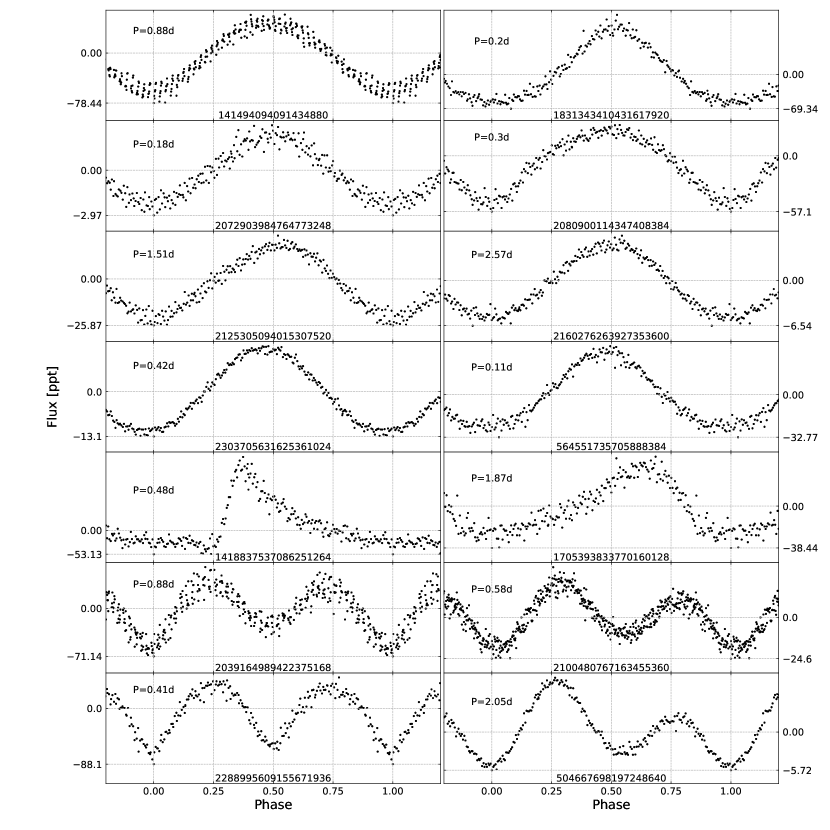
Figure 10: Phased time-series data of 14 (out of 93) spectroscopically unclassified binaries without sharp eclipses listed in Table 5. All plots are included in on-line material only.

Table 5: Basic information of 14 (out of 93) spectroscopically unclassified binaries without sharp eclipses. We show the time-series data of these objects in Figure 10. The full list of the objects in this group is included in on-line material.

		G		Period
Gaia DR2	TIC	[mag]	Sector	[days]	Remarks
One symmetric maximum detected – Figure 10
141494094091434880	67658009	13.0436	18	0.8764	-
1831343410431617920	406417817	14.7108	14	0.2010	crowded field
2072903984764773248	1879342714	17.8580	14	0.1761	crowded field
2080900114347408384	416641307	14.5962	14,15	0.3011	3 objects within 21"
2125305094015307520	21018674	13.4058	14,15,18,21,25,26	1.5079	-
2160276263927353600	233733792	12.4555	14-17,19-26	2.5694	-
2303705631625361024	397532904	12.8886	18,19,20,25,26	0.4204	-
564551735705888384	609725827	16.5793	18,19,24,25,26	0.1068	5 objects within 32"
One asymmetric maximum detected – Figure 10
1418837537086251264	1271027428	18.9619	17,20,23-26	0.4771	-
1705393833770160128	288381009	16.4297	14-26	1.8706	object 13" away
Two maxima detected – Figure 10
2039164989422375168	1712800054	16.6814	14	0.8764	crowded field
2100480767163455360	121107327	16.2609	14	0.5772	CV, Fontaine et al. (2011)
2288995609155671936	1884532373	16.5623	14-26	0.4107	-
504667698197248640	445526365	10.1176	18	2.0482	crowded field

We found 228 objects that are not spectroscopically classified and we identified neither as pulsators nor as eclipsing binary systems, presented earlier in this Section. This group includes objects that show peaks consistent with binarity but a small amplitude of a flux variation. The typical S/N is 8 or lower. We find these variations in amplitude spectra. This group also contains targets with multiple unrelated peaks in amplitude spectra, regardless of the S/N, which makes data phasing pointless. This multiplicity of peaks is typical for pulsators, however the amplitude spectra do not resemble the ones of sdBVs, since the unrelated peaks are below 60 $\upmu$Hz, and that is why we decided not to include them in Section 3.3. Gaia DR2 2105585421693855744 is identified with the cataclysmic variable V363 Lyr and reported by Scaringi et al. (2012). Gaia DR2 2127444125171341312 is very close to KIC 9278505 also reported by Scaringi et al. (2012). We provided basic information about these objects in Table 6, while we show the amplitude spectra in Figure 11.

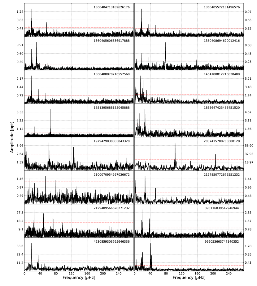
Figure 11: Amplitude spectra of 16 (out of 228) spectroscopically unclassified variables listed in Table 6. All plots are included in on-line material only.

Table 6: Basic information of 16 (out of 228) spectroscopically unclassified variables that we show in Figure 11. The full list is included in on-line material only.

		G
Gaia DR2	TIC	[mag]	Sector	Remarks
1360404713182626176	1270831583	15.8418	25,26	very crowded field
1360405572181496576	334899867	16.2057	25,26	very crowded field
1360405606536917888	1270837848	16.3565	25,26	very crowded field
1360408694620012416	334899806	16.1530	25,26	very crowded field
1360408870716557568	334899706	16.1600	25,26	very crowded field
1454780812716838400	1000656229	18.0202	23	very crowded field
1651395688155045888	1401049068	16.1897	14-25	-
1855647423465451520	1953033063	18.4158	14,15	2 bright objects within 21"
1979429038083843328	2011754031	15.2450	16	crowded field
2037415700780608128	1712233248	15.6530	14	3 bright objects within 21"
2100070954267036672	1715980555	17.7709	14	2 objects within 21"
2127850772675551232	1882665005	17.0644	15	object 19" away
2129409566628271232	290035516	16.0203	14,15	2 objects within 21"
398116839542946944	196946103	14.4348	17,18	object 16" away
4530859303765646336	1813173164	18.9596	26	5 objects within 21"
995053663747140352	444902249	10.8428	20	-

3.5 Non-sdB classified variables

Even though some of the objects in Geier (2020) are classified as non-sdB, we have included these in our search as well. These were first considered candidates for hot stars, but were identified as non-sdB objects, mostly O, B or A main sequence stars or white dwarfs. In total, we found 46 non-sdB variables. The same categories of flux variations emerged, with pulsator candidates, eclipsing binaries, reflection effect binaries, ellipsoidal variables, and classical pulsators, with the remaining objects having variability in their amplitude spectra. We present it likewise, i.e. pulsator candidates, eclipsing, reflection, ellipsoidal binaries, classical pulsator candidates, remaining objects with variability reported in their amplitude spectra. A table and figures of these objects are included in the on-line material only. The table includes basic information on each object along with additional references or contaminating objects, if any.

We found seven pulsator candidates with one being known before, i.e. Gaia DR2 2077737678383889408 reported by Reinhold et al. (2013). Among three eclipsing binaries with sharp eclipses, Gaia DR2 4322472232203849856, besides primary eclipse shows an additional flux drop between phase 0.75 and 1.0. The drop changes the phase, so it may be either two different drops or one drop that shifts from orbit to orbit. The phased time-series data do not show a secondary eclipse at phase 0.5, though a bit of a downward scatter exists. If it is a sign of the secondary eclipse the additional drop must be caused by a tertiary component. If, instead, the drop is the secondary eclipse, it shifts very quickly as a result of an apsidal motion. The extra drops phases well with both a period of 7.05325 days and its double. The Simbad database lists this object as a double or multiple star. A follow up photometry span over multiple orbits, should resolve this ambiguity. We found five more objects reported previously as variables. Four of them denoted KIC numbers have been observed with the the Kepler spacecraft and reported by Reinhold et al. (2013), while the last one is identified as an RS CVn variable by Drake et al. (2014).

4 Mode identification

We selected three objects where we are able to identify the pulsation modes by means of a rotational splitting and evenly spaced, in period, radial overtones, assuming these are g-mode sdBVs. The objects are the following, Gaia DR2 2129988841754560000, Gaia DR2 438585365733719168 and Gaia DR2 537697439806045824, and were selected since they have the richest amplitude spectra among all pulsator candidates we found.

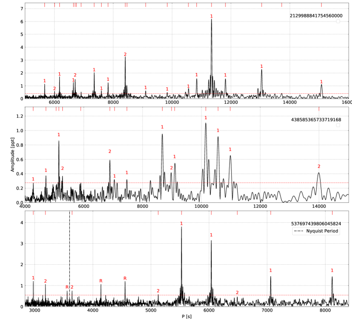
Figure 12: Amplitude spectra of three pulsators plotted in period. The red horizontal dashed lines denote $5\,\sigma$ detection threshold, which is consistent with FAP = 0.1% The modal degrees are shown on top of each detected peak. ‘R’ refers to reflection peaks across the Nyquist period.

We followed a standard prewhitening procedure by calculating an amplitude spectrum and removing consecutive peaks by fitting $A_{i}\sin(2{\pi}f_{i}t+{\phi_{i}})$ using a non-linear least-square method, where A_i is an amplitude, f_i is a frequency and $\phi_{i}$ is a phase of an i-th peak. We used our custom scripts for prewhitening. We removed all peaks down to a detection threshold of about S/N = 5. We updated this threshold level after each peak removal, hence the final threshold was calculated from the residual amplitude spectra, i.e. with all significant peaks removed. We present the lists of frequencies detected in each star in Tables 7, 8, and 9, while we show the amplitude spectra of these three stars in Figure 12.

Since stellar rotation splits pulsation modes into 2l+1 components of different m values, and often called multiplets, this splitting can be used for assigning the degree l of the split modes. One of the first examples with convincing rotationally split modes are Baran et al. (2009, 2012); Baran (2012). Besides the modal degree identification, a splitting itself is a direct measure of stellar rotation. These are two main reasons why the multiplets are so crucial for mode identification. Multiplets in sdBVs are not easily detectable. A common rotation period of sdBs is around 40 days, which means that data should cover at least 40 days, though preferentially 60 days, as was shown by Baran (2012). The three objects in our sample are two sector data only so our null result search for multiplets is of no surprise.

Another tool that has been widely used for a modal degree assignment is an asymptotic period spacing. In sdBVs, in the asymptotic regime i.e. $n\gg l$, consecutive overtones of gravity modes are equally spaced in period (e.g. Charpinet et al., 2000; Reed et al., 2011). Previous analysis of Kepler photometric data of sdBVs showed that the average period spacing of dipole modes is nearly 250 s (Reed et al., 2018). The period spacings for higher degree modes can be calculated using the following relation $\Delta$P_l = P₀/$\sqrt{l(l+1)}$.

Multiplet helps to constrain the modal degree and provides a head start for determining the asymptotic period spacing, as such three peaks are assigned l = 1 modes. In this work we could not rely on any multiplets and therefore we first focused on peaks that fit a sequence of l = 1 radial overtones. Such peaks should be separated by around 250 sec, not counting trapped modes. Peaks not satisfying our l = 1 period spacing sequence were assumed to be l = 2 modes or were unidentified l values if they have low amplitudes and do not fit the expected l = 2 spacing. We found no convincing candidates for trapped l = 1 modes. We stress though that without rotationally split modes, a modal degree assignment is not unique, since we try to fit an overtone sequence where some of the peaks may accidentally fit e.g. l = 1, while being a quadrupole mode or a higher degree mode. Besides multiplets, another help would come from a pulsation spectrum that is dense enough to complete at least the l = 1 sequence. We included the radial order and modal degree assignment in Tables 7 – 9. The average period spacings of dipole modes we estimated in these three stars are 247.22 (65) s (Gaia DR2 2129988841754560000), 208.70 (56) s (Gaia DR2 438585365733719168), 256.68 (1.02) s (Gaia DR2 537697439806045824). In the case of the first and third stars the average period spacing is close to the typical one found in sdBVs, while for the second star we found the spacing to be significantly lower. If this spacing is roughly correct it means that the core of Gaia DR2 438585365733719168 is denser comparing to a typical sdB star, which suggests a more evolved phase of its EHB evolution, with central helium abundance Y_c < 0.1.

Table 7: List of frequencies detected in an amplitude spectrum of Gaia DR2 2129988841754560000.

	Frequency	Period	Amplitude
ID	[$\upmu$Hz]	[s]	[ppt]	S/N	l	n
f1	66.327(7)	15076.8(1.7)	1.12(7)	12.4	1	60
f2	72.865(18)	13724.1(3.4)	0.45(7)	5.0	-	-
f3	76.6613(35)	13044.4(6)	2.29(7)	25.4	1	52
f4	84.658(6)	11812.2(9)	1.29(7)	14.3	1	47
f5	88.1774(13)	11340.78(17)	6.17(7)	68.5	1	45
f6	92.286(6)	10835.8(7)	1.35(7)	14.9	1	43
f7	94.737(11)	10555.5(1.2)	0.77(7)	8.5	1	42
f8	101.685(18)	9834.3(1.8)	0.44(7)	4.9	1	39
f9	109.870(15)	9101.7(1.3)	0.54(7)	6.0	1	36
f10	118.077(18)	8469.0(1.3)	0.46(7)	5.1	-	-
f11	118.9322(25)	8408.15(18)	3.29(7)	36.5	2	59
f12	127.776(6)	7826.19(36)	1.38(7)	15.4	1	31
f13	131.620(13)	7597.6(7)	0.65(7)	7.2	1	30
f14	135.9947(38)	7353.23(21)	2.14(7)	23.7	1	29
f15	144.718(17)	6910.0(8)	0.47(7)	5.2	-	-
f16	148.195(16)	6747.9(7)	0.53(7)	5.9	-	-
f17	149.1444(48)	6704.91(21)	1.72(7)	19.1	2	47
f18	150.457(6)	6646.40(27)	1.33(7)	14.8	1	26
f19	161.9192(47)	6175.92(18)	1.73(7)	19.2	1	24
f20	166.472(14)	6007.0(5)	0.58(7)	6.4	2	42
f21	176.355(7)	5670.37(24)	1.10(7)	12.2	1	22

Table 8: List of frequencies detected in an amplitude spectrum of Gaia DR2 438585365733719168.

	Frequency	Period	Amplitude
ID	[$\upmu$Hz]	[s]	[ppt]	S/N	l	n
f1	20.449(45)	48902(106)	0.42(5)	7.7	-	-
f2	71.436(46)	13998.5(9.0)	0.41(5)	7.4	2	117
f3	91.073(26)	10980.2(3.2)	0.72(5)	13.1	1	52
f4	94.650(21)	10565.3(2.3)	0.91(5)	16.6	1	50
f5	98.520(17)	10150.2(1.7)	1.14(5)	20.7	1	48
f6	110.033(34)	9088.2(2.8)	0.61(6)	11.2	1	43
f7	111.318(47)	8983.3(3.8)	0.45(6)	8.2	2	75
f8	115.338(19)	8670.2(1.5)	0.98(5)	17.8	1	41
f9	133.94(6)	7466.2(3.1)	0.34(5)	6.2	1	35
f10	141.89(6)	7047.5(2.8)	0.34(5)	6.1	1	33
f11	145.221(31)	6886.1(1.5)	0.62(5)	11.2	2	57
f12	169.58(6)	5897.0(2.1)	0.31(5)	5.6	-	-
f13	189.46(6)	5278.2(1.6)	0.34(5)	6.1	2	43
f14	194.110(22)	5151.7(6)	0.88(5)	16.0	1	24
f15	197.67(7)	5058.8(1.7)	0.29(5)	5.3	-	-
f16	212.247(48)	4711.5(1.1)	0.40(5)	7.2	1	22
f17	233.52(7)	4282.3(1.2)	0.28(5)	5.0	1	20

Table 9: List of frequencies detected in an amplitude spectrum of Gaia DR2 537697439806045824.

	Frequency	Period	Amplitude
ID	[$\upmu$Hz]	[s]	[ppt]	S/N	l	n
f1	123.167(8)	8119.0(5)	1.37(9)	12.6	1	31
f2	141.626(7)	7060.86(35)	1.56(10)	14.4	1	27
f3	154.153(22)	6487.1(9)	0.51(10)	4.7	2	43
f4	165.5908(34)	6038.98(13)	3.18(9)	29.4	1	23
f5	180.9512(29)	5526.35(9)	3.84(10)	35.4	1	21
f6	195.113(20)	5125.2(5)	0.56(10)	5.1	2	34
f7	274.501(13)	3642.97(17)	0.85(9)	7.8	2	24
f8	313.988(11)	3184.84(11)	1.00(10)	9.2	2	21
f9	336.018(9)	2976.03(8)	1.21(10)	11.2	1	11

5 Orbital period stability

In total we found 33 eclipsing binary systems with sharp eclipses. Such eclipses are very suitable for deriving an orbital period and checking its stability that provides insights into physical effects in the systems, e.g. evolutionary changes (mass loss or mass exchange between components, tidal dissipation effects, gravitational radiation, magnetic braking), light travel time variation (stellar pulsations, a shift of the secondary eclipse, additional body in a system, apsidal motion). These effects alter the orbital period on a long time scale. In eclipsing binary systems orbital periods can be calculated from mid-times of primary or secondary eclipses. To estimate the mid-times we used the method described by Kwee & van Woerden (1956). Then, we fit the orbital periods to the mid-times and calculated the Observed-minus-Calculated (O-C) diagrams. The O-C diagram is a very effective tool to measure orbital period variation, if any, and a shape of a variation helps indicate its source. The interpretation of the shape is explained by Sterken (2005).

Most of the selected eclipsing binaries in our sample show stable periods within the errors. It means that either the period does not change on a time scale comparable to the time coverage of our data or the change is too small to be detectable in the data. The typical time coverage of our data is only one month (one-sector). Out of 33 systems only in case of 12 the S/N ratio of the data is high enough to derive reasonable period estimation. We present the periods and the reference epochs, defined as a mid-time of one of the eclipses, in Table 10. In case of 10 systems the O-C diagrams show no variation within the errors, while in the case of two systems, Gaia DR2 1816806183083980288 and Gaia DR2 2086140799075771520, the variations look significant (Figure 13). We stress however that the errors of mid-times calculated using the method reported by Kwee & van Woerden (1956) are underestimated, hence the true ones can be larger making the variations insignificant. The shapes and the physical reasons of these variations, if real, are not clear and require longer coverage to make any conclusive implications.

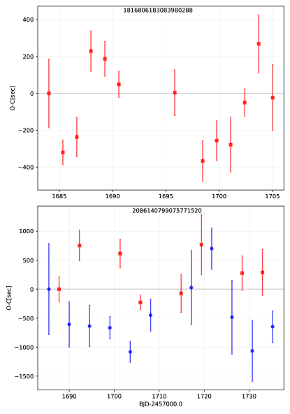
Figure 13: Top panel shows the O-C diagram of Gaia DR2 1816806183083980288. All eclipses are considered primary. Bottom panel shows the O-C analysis of Gaia DR2 2086140799075771520. Mid-times of primary eclipses are plotted with red squares, while of secondary eclipses with blue circles.

Table 10: Ephemerides of a selected sample of eclipsing binaries, calculated from mid-times of primary eclipses.

	Period	T0
Gaia DR2	[days]	[days]
2129388572827118720	1.23135725(49)	2458684.75482(12)
190164354254168192	2.34580(14)	2458817.8620(8)
1816806183083980288	1.31229(17)	2458684.0236(6)
1846629538332584960	0.8097(1)	2458711.2610(9)
2093326416800046848	4.1776590(9)	2458684.29845(44)
450362269138662400	3.4574(9)	2458792.6052(27)
967312053368970624	3.185675(7)	2458843.19265(35)
1831073927011326720	7.47899(39)	2458681.13135(50)
2086140799075771520	4.5233(5)	2458683.2089(31)
1821225425253990400	1.177035(9)	2458683.7224(12)
431584053656962816	6.3148495(40)	2458765.19978(15)
4322472232203849856	3.4800(6)	2458684.5481(18)

6 Summary

In Paper I we reported our result of the search for sdBVs in the southern ecliptic hemisphere observed by TESS satellite and we detected two convincing cases, while the remaining 26 sdBs turned out to be variable, and in most cases their binary nature causes the variations. The total number of variables found was 1807. In this work, we have continued our effort to search for sdBVs across the sky using TESS satellite. In total, we found 506 variables, among which 13 are likely sdBV stars, while another 40 sdBs show other types of variability, most from being in a binary system. One of them shows HW Vir shape of the phased time-series data. We found another five objects showing HW Vir variations among spectroscopically unclassified, bringing the final number of new HW Vir systems to seven (if all of them are confirmed to be sds). Comparing the number of new sdB variable objects, we can notice that even though the number of all objects, available in Geier (2020), and consequently the total number of new variables, was larger in the southern ecliptic hemisphere, we found more variable sdBs, including sdBVs, in the northern ecliptic hemisphere. Since, we rejected objects observed in the short cadence mode, we cannot conclude on the larger number of them in the north, but it clearly means there was still more to find.

Summing up all variable stars we found in the TESS field of view, we arrive with the following numbers: 15 likely sdBVs, 66 variable non-pulsating sdBs, 33 variable sds, 2076 spectroscopically unclassified objects (including 113 objects that show peaks in the sdBV g-mode region), 123 non-sdB variables. The ultimate goal of our work was to discover missing sdBVs to contribute to the completeness of the sdBV sample in the TESS mission. The byproduct of our findings is additional objects for the short cadence observations (either 2 min or 20 sec) during the second run of TESS in the southern and northern ecliptic hemispheres. The extra runs can deliver more precise data for further astrophysical analysis. Another byproduct will be pushing the Nyquist frequency beyond the p-mode region in sdBVs. For now, our search is limited to g-mode sdBVs, which is a consequence of the 30 min. cadence, however the search utilizes the most updated sdB database along with the all-sky space survey, allowing for the most complete sample of g-mode sdBVs currently possible. Spectroscopic classification is needed to confirm 113 objects that show sdBV-like amplitude spectra, as well as all sds variables and the massive number of other unclassified variables.

The sdBVs we found in this work are not rich in g-modes that is why are not best cases for any mode identification. However, likewise in Paper I, among objects that are not confirmed sdBs but show typical g-mode sdBV amplitude spectra, we have selected three objects best-suited for the mode identification. They show the richest amplitude spectra. We searched for multiplets and found none, therefore we used only period spacing for the modal degree assignment. The sequences of presumably same degree overtones are not too complete but the multiples of 250 sec (ish) was still found. This may be another argument for these objects being sdB stars. One of the stars shows 208 sec spacing which is either an indication of a denser core or incorrect assumption that the star is an sdB. Our identification will only be reliable if these objects are spectroscopically confirmed to be sdBs.

We selected a sample of 12 eclipsing binary systems with sharp eclipses and derived mid-times of eclipses in order to calculate O-C diagrams. We measured orbital periods and checked their stabilities. Out of 12 systems only two show significant O-C variation, within the given errors, suggesting that some period change may be present in those systems. This conclusion is uncertain as the errors are underestimated, and longer data coverage is needed to make any physical interpretations.

Data availability

The datasets were derived from MAST in the public domain archive.stsci.edu.

References

- Baran (2012) Baran A., 2012, AcA, 62, 179
- Baran et al. (2009) Baran A., et al., 2009, MNRAS, 392, 1092
- Baran et al. (2012) Baran A. S., et al., 2012, MNRAS, 424, 2686
- Baran et al. (2015) Baran A. S., Koen C., Pokrzywka B., 2015, MNRAS, 448, 16
- Baran et al. (2019) Baran A., Telting J., Jeffery C., Østensen R., Vos J., Reed M., Vučković M., 2019, MNRAS, 489, 1556
- Bond et al. (1978) Bond H. E., Liller W., Mannery E. J., 1978, ApJ, 223, 252
- Brasseur et al. (2019) Brasseur C. E., Phillip C., Fleming S. W., Mullally S. E., White R. L., 2019, Astrocut: Tools for creating cutouts of TESS images (ascl:1905.007)
- Charpinet et al. (1997) Charpinet S., Fontaine G., Brassard P., Chayer P., Rogers F. J., Iglesias C. A., Dorman B., 1997, ApJ, 483, 123
- Charpinet et al. (2000) Charpinet S., Fontaine G., Brassard P., Dorman B., 2000, ApJS, 131, 223
- Drake et al. (2014) Drake A. J., et al., 2014, The Astrophysical Journal Supplement Series, 213, 9
- Feinstein et al. (2019) Feinstein A. D., et al., 2019, Publications of the Astronomical Society of the Pacific, 131, 094502
- Fontaine et al. (2003) Fontaine G., Brassard P., Charpinet S., Green E., Chayer P., Billères M., Randall S., 2003, ApJ, 597, 518
- Fontaine et al. (2011) Fontaine G., et al., 2011, The Astrophysical Journal, 726, 92
- Geier (2020) Geier S., 2020, A&A, 635, A193
- Heber (2016) Heber U., 2016, PASP, 128, 2001
- Holdsworth et al. (2017) Holdsworth D. L., Østensen R. H., Smalley B., Telting J. H., 2017, Monthly Notices of the Royal Astronomical Society, 466, 5020
- Kilkenny et al. (1997) Kilkenny D., Koen C., O’Donoghue D., Stobie R. S., 1997, Monthly Notices of the Royal Astronomical Society, 285, 640
- Kwee & van Woerden (1956) Kwee K., van Woerden H., 1956, Bulletin of the Astronomical Institutes of the Netherlands, 12, 327
- Lightkurve Collaboration et al. (2018) Lightkurve Collaboration et al., 2018, Lightkurve: Kepler and TESS time series analysis in Python, Astrophysics Source Code Library (ascl:1812.013)
- Østensen et al. (2011) Østensen R. H., et al., 2011, MNRAS, 414, 2860
- Randall et al. (2009) Randall S., van Grootel V., Fontaine G., Charpinet S., Brassard P., 2009, A&A, 507, 911
- Reed et al. (2011) Reed M. D., et al., 2011, MNRAS, 414, 2885
- Reed et al. (2012) Reed M. D., Baran A., Østensen R. H., Telting J. H., O’Toole S. J., 2012, MNRAS, 427, 1245
- Reed et al. (2018) Reed M., et al., 2018, Open Astronomy, 27, 157
- Reinhold et al. (2013) Reinhold T., Reiners A., Basri G., 2013, A&A, 560, A4
- Sahoo et al. (2020) Sahoo S., Baran A., Sanjayan S., Ostrowski J., 2020, MNRAS, 499, 5508
- Scaringi et al. (2012) Scaringi S., Groot P. J., Verbeek K., Greiss S., Knigge C., Körding E., 2012, Monthly Notices of the Royal Astronomical Society, 428, 2207
- Sterken (2005) Sterken C., 2005, in Sterken C., ed., Astronomical Society of the Pacific Conference Series Vol. 335, The Light-Time Effect in Astrophysics. p. 3
- Taylor (2005) Taylor M. B., 2005, TOPCAT & STIL: Starlink Table/VOTable Processing Software. p. 29
- Wenger et al. (2000) Wenger M., et al., 2000, Astron. Astrophys. Suppl. Ser., 143, 9