Highly viscous electron fluid in GaAs quantum wells

Abstract

A fluid in which shear-stress transverse waves, being character for solids, can propagate is usually referred as a highly viscous fluid. Hydrodynamics of the fluid formed by conduction electrons has been recently discovered in graphene Levitov_et_al ; graphene_1 ; graphene_2 ; graphene_4 ; graphene_5 ; Polini_Geim , ultra-pure Weyl and layered metals Moll ; Gooth , and high-mobility GaAs quantum wells exps_neg_1 ; exps_neg_2 ; exps_neg_3 ; exps_neg_4 ; je_visc ; Gusev_1 ; recentest_ . Here we construct a theory of magnetotransport in a highly viscous two-dimensional (2D) electron fluid in moderate magnetic fields, accounting its viscoelastic dynamics and the memory effects in the interparticle scattering. In addition to the properties of the microwave-induced resistance oscillations (MIRO) in photoresistance explained by theories theor_1 ; theor_1_1 ; theor_2 ; joint ; Polyakov_et_al_classical_mem ; Beltukov_Dyakonov for non-interacting 2D electrons, our theory predicts an irregular shape of MIRO at certain sample sizes, a peak in photoresistance near the doubled electron cyclotron frequency, and no dependence of MIRO on the helicity of the circular polarization of radiation. These effects, which are the evidences of the excitation of the transverse magnetosonic waves, were observed in magnetotransport experiments Smet_1 ; Ganichev_1 ; exp_GaAs_ac_1 ; exp_GaAs_ac_2 ; exp_GaAs_ac_3 ; recentest_ on ultra-high-quality GaAs quantum wells. We conclude that 2D electrons in such structures in magnetic field form a highly viscous fluid.

1. Introduction. Microwave-induced resistance oscillations (MIRO) of 2D electrons in high-mobility conductors in moderate magnetic fields is an intriguing effect, whose correct explanation is, apparently, crucial for understanding of the nature of transport phenomena in such systems. MIRO was initially observed exp_1 ; exp_2 ; exp_3 and then extensively studied rev_M in GaAs quantum wells.

Originally, MIRO were attributed to transitions of non-interacting 2D electrons at high Landau levels in external dc and ac electric fields theor_1 ; theor_1_1 ; theor_2 ; joint . Such “displacement mechanism” Ryzhii ; Ryzhii_Suris is based on taking into account the radiation-assisted scattering of 2D electrons in quantized states on disorder, that result in unequal probabilities of electron transitions in the opposite directions at a dc field. Theories theor_1 ; theor_1_1 yield the correct profile of the magnetooscillations of photoresistance in not very clean samples. In Ref. theor_2 the “inelastic mechanism” was proposed in which the crucial role is played by radiation-induced redistribution of electrons by energy. Its contribution to photoresistance explains the temperature dependence of MIRO. The classical memory effects in scattering of 2D electrons on disorder also can lead to magnetooscillations in photoresistance Polyakov_et_al_classical_mem .

In Ref. Beltukov_Dyakonov a different powerful approach to the theory of MIRO was developed. It is based on a phenomenological description of the memory effects in classical dynamics of non-interacting 2D electrons, scattered on localized defects. Theory Beltukov_Dyakonov , supported by numerical experiments (their results are presented also in Ref. Beltukov_Dyakonov ), describes MIRO in a self-consistent and lucid way.

Theories theor_1 ; theor_1_1 ; theor_2 ; joint ; Polyakov_et_al_classical_mem ; Beltukov_Dyakonov have a substantial problem which is the inconsistency between an almost full lack of dependence of the effect on the sign of the circular polarization of radiation in some experiments Smet_1 ; Ganichev_1 and the need to involve special factors of experimental setup rev_M ; Savchenko or very special models of electron dynamics Mikhailov ; Chepelianskii_Shepelyansky to explain this lack in theory. Moreover, in best-quality GaAs quantum wells were observed Smet_1 ; Ganichev_1 ; exp_GaAs_ac_1 ; exp_GaAs_ac_2 peculiar features of MIRO, a non-sinusoidal profile and a giant peak near the doubled cyclotron frequency, unexplained within disorder-based theories.

In parallel with the studies of MIRO, the giant negative magnetoresistance was observed in the same high-mobility GaAs quantum wells exps_neg_1 ; exp_GaAs_ac_1 ; exps_neg_2 ; exps_neg_3 ; exps_neg_4 ; Gusev_1 ; recentest_ . In Ref. je_visc it was explained as the result of formation of a viscous fluid from 2D electrons in the quantum wells Gurzhi_Shevchenko . Later, a very similar huge negative magnetoresistance was detected in other high-quality conductors: 2D metal PdCoO₂ Moll , the 3D Weyl semimetal WP₂ Gooth , and single-layer graphene graphene_4 ; graphene_5 , for which other evidences of the hydrodynamic electron transport were already discovered.

In Refs. vis_res_1 it was pointed out that the high-frequency viscosity coefficients of 2D electrons exhibit a resonance at the twice cyclotron frequency related to the perturbations of the shear stress in the fluid. In the case of a highly viscous fluid, such “viscoelastic” resonance manifests itself via the transverse magnetosonic waves vis_res_2 ; Semiconductors . We qualitatively argued in Ref. vis_res_2 that this effect is responsible for the peak and the anomalies observed in ac magnetotransport near the doubled cyclotron frequency in the high-quality GaAs quantum wells exp_GaAs_ac_1 ; exp_GaAs_ac_2 ; exp_GaAs_ac_3 ; recentest_ .

In this work we construct a phenomenological theory of non-linear magnetotransport in a highly viscous 2D electron fluid. Following to the approaches of Refs. Beltukov_Dyakonov ; vis_res_2 , we formulate macroscopic motion equations for such fluid. They are the Drude-like viscoelastic equations of Ref. vis_res_2 supplemented by the retarded relaxation terms accounting the classical memory effects in the interparticle scattering and in the interaction energy. The calculated photoconductivity of a Poiseuille flow exhibits magnetooscillations and a peak at the doubled cyclotron frequency. The magnetooscillations can have a sinusoidal or an irregular shape depending on the sample widths. Such shape as well as the peak are induced by the viscoelastic resonance and excitation of the standing magneosonic waves. For circularly polarized radiation, the photoconductivity is independent of the helicity of the polarization. All these effects were observed in high-quality GaAs quantum wells Smet_1 ; Ganichev_1 ; exp_GaAs_ac_1 ; exp_GaAs_ac_2 ; exp_GaAs_ac_3 ; recentest_ . In this way, our results evidence that 2D electrons in best-quality GaAs quantum wells form a highly viscous fluid at moderate magnetic fields. We emphasize that microscopic structure of this highly-correlated electron phase and the condition of its realization is to be further studied.

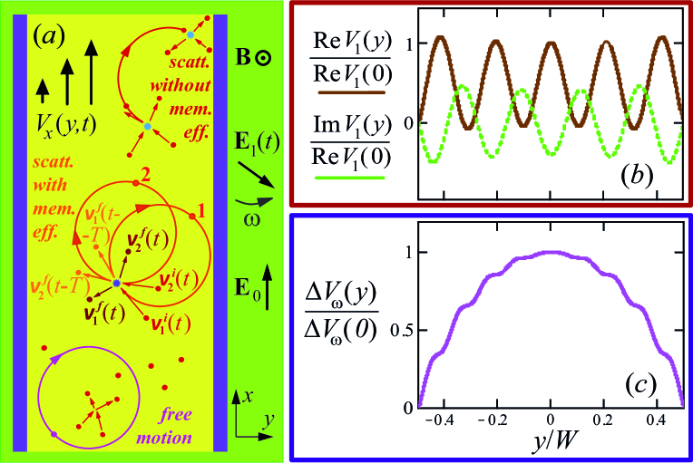
Figure 1: ($a$) Flow of a highly viscous 2D electron fluid in a long defectless sample with rough edges in a magnetic field $\mathbf{B}$, a dc electric field $\mathbf{E}_{0}$, and a circularly polarized radiation field $\mathbf{E}_{1}(t)$. Trajectories of two Fermi liquid quasiparticles in an extended collision, leading to the memory effect, as well as trajectories of a collisionless motion and of two successive collisions without the memory effect are drawn. ($b$) Ac component $V_{1}(y)\sim E_{1}$ of the fluid velocity in the long sample shown in panel (a). ($c$) Radiation-induced correction $V_{\omega}(y)\sim E_{0}E_{1}^{2}$ to the dc flow component $V_{0}(y)\sim E_{0}$ in the same sample. All curves are plotted for the parameters: $\omega\tau_{2}=40$, $\tau_{q}/\tau_{2}=0.7$, $W/L_{s}=1$, and $\omega_{c}/\omega=0.34$. The wavelength and the decay length of magnetosonic waves are: $0.21\,W$ and $1.0\,W$.

2. Model. At high frequencies, $\omega\gg 1/\tau_{2}$, a flow of a highly viscous 2D electron fluid in magnetic field is formed by magnetoplasmons related to perturbations of the electron density $n$ and by the transversal magnetosonic waves related to perturbations of the shear stress vis_res_2 . The last ones are governed by the dissipativeless part of interparticle interaction, described by the Landau interaction term within the Fermi-liquid model Semiconductors . The interparticle scattering leads to a weak relaxation of both the plasmonic and the viscoelastic flow components. The Navier-Stokes equation of the 2D electron fluid at a strong interparticle interaction (large Landau parameters, $F_{m}\gg 1$) were derived in Ref. el for zero magnetic field and in Ref. Semiconductors for a nonzero magnetic field. Apparently, the consideration of Refs. vis_res_2 ; Semiconductors is qualitatively valid also for a moderately nonideal electron fluid, in which $F_{m}\sim 1$, We even hypothesize that the viscoelastic dynamics can be realized even in flows of a weakly non-ideal Fermi gas due to the appearance of strong correlations in the motion of electrons in magnetic field. These correlations are related to the memory effects in the interparticle scattering induced by subsequent collisions of two electrons, joined in “pairs” {see Fig. 1($a$), for details see Supplemental Information SI }.

The formation of such pairs of electrons (more exactly, quasiparticles of the electron fluid) is also induces non-local by time effects in fluid dynamics. These memory effects are analogous to the subsequent “extended” collisions of non-interacting 2D electrons with localized defects in magnetic field Beltukov_Dyakonov . Here we account the memory effects in the electron fluid induced by the quasiparticle pairs by adding the non-linear retarded terms in the fluid dynamic equations. These terms are the interparticle scattering term, similar to the retarded electron-disorder scattering term from Ref. Beltukov_Dyakonov , and the perturbation term of the Landau interaction parameter $F_{2}$, accounting retarded correction of the elastic part of the interparticle interaction. The resulting equations for the density $n$, the velocity $\mathbf{V}$, and the momentum flux $\hat{\Pi}$, extending the equations from je_visc ; vis_res_2 ; Semiconductors , take the form:

$$\begin{array}[]{l}\displaystyle\partial n/\partial t\,+\,n_{0}\,\mathrm{div}\mathbf{V}\,=\,0\,,\\ \\ \displaystyle\partial V_{i}/\partial t\,=\,eE_{i}/m+\omega_{c}\epsilon_{ikz}V_{k}-(1/m)\,\partial\Pi_{ij}/\partial x_{j}\,,\\ \\ \displaystyle(1+\delta F_{2,\,ij})^{-1}\,\partial\Pi_{ij}/\partial t\,=\,2\omega_{c}\epsilon_{ikz}\Pi_{kj}\,-\\ \\ \displaystyle\;\;\quad-\Pi_{ij}/\tau_{2}-m(v_{F}^{\eta})^{2}\,V_{ij}/4-\Gamma_{ijkl}\,\Pi_{kl}(\mathbf{r},t-T)\,.\end{array}$$ (1)

Here $n_{0}=n-\delta n$ is the equilibrium density of quasiparticles; the electric field $\mathbf{E}=\mathbf{E}(\mathbf{r},t)$ consists of the applied field and the internal field induced by a non-equilibrium charge density $e\,\delta n(\mathbf{r},t)$: $\mathbf{E}(\mathbf{r},t)=\mathbf{E}^{ext}(t)+\mathbf{E}^{int}(\mathbf{r},t)$; $e$ and $m$ are the electron charge and the effective mass; $\epsilon_{ikm}$ is the antisymmetric unit tensor; $V_{ij}=\partial V_{i}/\partial x_{j}+\partial V_{j}/\partial x_{i}$; $\tau_{2}$ is the shear stress relaxation time without the memory effects; $v^{\eta}_{F}$ is the parameter defining the magnitude of the viscosity $\eta$ of a highly viscous fluid vis_res_2 : $\eta|_{B=0}=(v_{F}^{\eta})^{2}\tau_{2}/4$; $\delta F_{2,\,ij}$ are the retarded perturbations of the Landau parameter $F_{2}$; and $T=2\pi/\omega_{c}$ is the cyclotron period. The values $n_{0}$, $m$, $\tau_{2}$, and $v_{F}^{\eta}$ are expressed via the Landau parameters $F_{0}$, $F_{1}$, and $F_{2}$ Semiconductors .

The term $-\Gamma_{ijkl}(\mathbf{r},t)\Pi_{kl}(\mathbf{r},t-T)$ in Eq. (1) describes the retarded relaxation of $\Pi_{ij}$ due to the extended collisions of pairs of quasiparticles with one return to the same point [see Fig. 1($a$)]. Extended collisions are sensitive to the macroscopic motion of the fluid via the forces acting on quasiparticles from the internal field $\mathbf{E}^{int}$ and from the elastic tension. The latter one is induced by perturbations of the quasiparticle energy spectrum by nonzero $\mathbf{V}$, which is expressed via the term $-m(v_{F}^{\eta})^{2}V_{ij}/4$ el ; Semiconductors . Because of these sensitivity, the tensor $\hat{\Gamma}(\mathbf{r},t)$ depends on the variables characterizing the fluid in the past, $t^{\prime}<t$.

At rare interparticle collisions, when $\omega_{c}\tau_{2}\gg 1$, the tensor $\Gamma_{ijkl}(\mathbf{r},t)$ depends mainly on the shift of the strain tensor, $\varepsilon_{mn}=\partial u_{m}/\partial x_{n}+\partial u_{n}/\partial x_{m}$, in one cyclotron period: $\Delta_{mn}(\mathbf{r},t)=\varepsilon_{mn}(\mathbf{r},t)-\varepsilon_{mn}(\mathbf{r},t-T)$ {$\mathbf{u}(\mathbf{r},t)$ is the displacement of small fluid elements, for details see SI }. For a small-amplitude flow, the tensor $\hat{\Gamma}=\hat{\Gamma}(\hat{\Delta})$ is expanded into power series by $\hat{\Delta}$:

$$\begin{array}[]{c}\displaystyle\Gamma_{ijkl}[\mathbf{u}(\mathbf{r}^{\prime},t)^{\prime}]=\Gamma^{(0)}_{ijkl}+\alpha_{ijkl}^{mnop}\,\Delta_{mn}\,\Delta_{op}\>,\end{array}$$ (2)

where the coefficients $\Gamma^{(0)}_{ijkl}$ and $\alpha_{ijkl}^{mnop}$ are proportional to the probability $P=e^{-T/\tau_{q}}$ to make a full cyclotron rotation without collisions with other quasiparticles (here $\tau_{q}\lesssim\tau_{2}$ is the interparticle departure scattering time).

The factor $(1+\delta F_{2,ij})^{-1}$ in Eq. (1) originates from the renormalization of the quasiparticle energy spectrum by the inter-particle interaction in an electron Fermi liquid. We propose that the magnitude of the Landau interaction parameter $F_{2}$ is changed on the value $\delta F_{2,ij}=\delta F_{2,ij}[\,\mathbf{V}(\mathbf{r}^{\prime},t^{\prime})\,]\sim V^{2}$ due to a perturbation of the quasiparticle interaction energy in an inhomogeneous flow SI . For simplicity, in the left side of Eq. (1) we neglect the factor $1/(1+F_{2})$ near $\delta F_{2,ij}$ as it do not lead to qualitative changes of results SI . Owing a semi-deterministic character of particle dynamics at $t^{\prime}<t$, the value $\delta F_{2,ij}$ depends on the velocity $\mathbf{V}$ in the current moment $t$ as well as in the retarded moments $t^{\prime}=t-nT$, $n=1,2,..$, when two quasiparticles, moving by cyclotron trajectories, were located near their positions at $t=0$ with a large probability [see Fig. 1($a$)]. We account only one cyclotron returning, so we consider that $\delta F_{2,ij}^{(1)}(\mathbf{r},t)=\delta F_{2,ij}^{(1)}[\,\mathbf{V}(\mathbf{r},t-T)\,]$ SI .

The magnitude of $\delta F_{2,ij}^{(1)}$ is considered to be proportional to the energy absorbed in the moment $t^{\prime}=t-T$ by the flow from the external electric field, $W=V_{kl}\Pi_{kl}$, and other linear combinations of $\mathbf{V}$ and $\hat{\Pi}$:

$$\begin{array}[]{c}\displaystyle\delta F_{2,ij}^{(1)}[\mathbf{V}(\mathbf{r}^{\prime},t^{\prime})]=\beta_{ij}^{klps}\,V_{kl}(\mathbf{r},t-T)\Pi_{ps}(\mathbf{r},t-T)\,,\end{array}$$ (3)

where $\beta_{ij}^{klmn}$ are the coefficients, which are proportional to the probability $P$, like as the coefficients $\Gamma_{ijkl}$ SI .

In this way, we have accounted the inelastic and the elastic nonlinear effects in the fluid dynamics originating from the interparticle scattering and from the interparticle interaction energy by the terms $-\Gamma_{ijkl}\Pi_{kl}(\mathbf{r},t-T)$ [Eq. (2)] and $-\delta F_{2,ij}^{(1)}\,\partial\Pi_{ij}/\partial t$ [Eq. (3)], respectively.

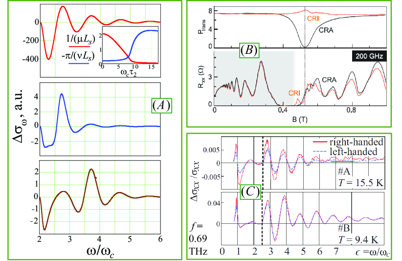
Figure 2: ($A$) Calculated relaxation contribution to photoconductivity $\Delta\sigma_{\omega}^{rel}$ due to the memory effect in the interparticle scattering for Poiseuille flows with the parameters $\omega\tau_{2}=17$; $\tau_{q}/\tau_{2}=0.7$; $W/L_{s}=5.5,\,0.85,\,0.66$ for the upper, center, and lower subpanels, respectively. Inset: the dependencies of the length of decay ($1/\mu$) and one half of the wavelength ($-\pi/\nu$) of magnetosonic waves on the value $\omega_{c}\tau_{2}\sim B$ at $\omega\tau_{2}=17$ in the diapason $0<\omega_{c}<\omega$. ($B$) Experimental data of Ref. Smet_1 on the cyclotron resonance in absorption (upper subpanel) and MIRO (lower subpanel) in an ultra-high quality GaAs quantum well with the experimental value of “mean sample mobility” $\mu=18\cdot 10^{6}$ cm${}^{2}/$V$\cdot$s. Red and black curves refer to the inactive and the active circular polarizations of radiation. ($C$) Experimental data of Ref. Ganichev_1 on oscillating photoconductivity, analogous to MIRO, for two GaAs quantum wells: with a moderate experimental mobility (sample $\#$A with $\mu=0.82\cdot 10^{6}$ cm${}^{2}/$V$\cdot$s, upper subpanel) and with a higher experimental mobility (sample $\#$B with $\mu=1.8\cdot 10^{6}$ cm${}^{2}/$V$\cdot$s, lower subpanel). Red and blue curves refers to the right and the left circular polarizations.

3. Photoconductivity of Poiseuille flow. We consider a Poiseuille flow in a defectless long sample as a minimal model to study the effect of radiation on magnetotransport in a highly viscous 2D electron fluid [see Fig. 1($a$)].

The external electric field $\mathbf{E}^{ext}(t)=\mathbf{E}_{0}+\mathbf{E}_{1}(t)$ consist of the dc field $\mathbf{E}_{0}=E_{0}\,\mathbf{e}_{x}$ induced by an applied electric bias and the radiation field $\mathbf{E}_{1}(t)=\mathbf{E}_{1}^{\pm}e^{-i\omega t}+c.c.$ with the left or the right circular polarizations: $\mathbf{E}_{1}^{\pm}=E_{1}\,(\,1/2\,,\,\pm i/2\,)$. The sample edges are supposed to be rough, thus the diffusive boundary conditions, $\mathbf{V}|_{y=\pm W/2}=0$, are applicable. The internal field $\mathbf{E}^{int}(y,t)$ in this geometry is directed along the $y$ axis, being the Hall field. For simplicity, the sample is considered to be very narrow: $W\ll l_{p}$, where $l_{p}$ is the characteristic plasmon wavelength. In such case, the field $\mathbf{E}^{int}(y,t)$ screens the $y$ component of the incident ac field $\mathbf{E}_{1}(t)$, thus the ac plasmonic flow component, related to the charge density $e\delta n(y,t)$, is suppressed and the ac component of the flow is formed mainly by the viscoelastic eigenmodes vis_res_2 ; SI . Herewith only the $x$ component of the hydrodynamic velocity $\mathbf{V}$ and the $xy$ component of the tensors $V_{ij}$ and $\varepsilon_{ij}$ presents in both the ac and the dc flow components.

Within formulated model [equations (1)-(3)], we calculate the linear, $V_{0,1}(y,t)\sim E_{0,1}$, and the nonlinear, $V_{\omega}(y)\sim E_{1}^{2}E_{0}$, responses of the fluid in the described setup on the dc and ac fields $\mathbf{E}_{0}$ and $\mathbf{E}_{1}(t)$. In Fig. 1($b$,$c$) we draw the profiles of the amplitude $V_{1}(y)$ of the ac velocity $V_{1}(y,t)=V_{1}(y)\,e^{-i\omega t}+c.c.$ and the nonlinear dc component $V_{\omega}(y)$ in a sample which is much wider than the characteristic magnetosonic wavelength $l_{s}$ and comparable with the characteristic decay length $L_{s}$. The ac-field-induced correction to the dc velocity $V_{\omega}(y)$ inherits both the oscillations of $V_{1}(y)$ by $y$, related to standing magnetosonic waves [see panel (c)], as well as the parabolic profile of the dc Poiseuille flow $V_{0}(y)\sim E_{0}[(W/2)^{2}-y^{2}]$.

The resulting mean sample photoconductivity $\Delta\sigma_{\omega}$ does not depend on the sign “$\pm$” of the circular polarization of $\mathbf{E}_{1}(t)$. Indeed, we have mentioned above that in narrow samples, $W\ll l_{p}$, the ac linear response $V_{1}(y,t)$, mainly formed by the viscoelastic contribution, is independent of the sign $\pm$ due to the screening of the $y$ component of the incident field $\mathbf{E}_{1}(t)$ by the internal field $\mathbf{E}^{int}\sim\delta n$. Thus the nonlinear components of the velocity, $V_{\omega}^{rel}$ and $V_{\omega}^{el}$, stemming from the retarded inelastic relaxation term, $\sim\Gamma_{ijkl}$, as well as from the retarded elastic interaction terms, $\sim\delta F_{2,ij}$, are also independent of the sign $\pm$.

In Fig. 2($A$) we show the contribution to photoconductivity $\Delta\sigma^{rel}_{\omega}\sim V_{\omega}^{rel}$ from the relaxation memory term $\sim\Gamma_{ijkl}$. It is seen that the magnetooscillations of $\Delta\sigma_{\omega}^{rel}$ are regular (sinusoidal with damping) in relatively wide samples: $W\gg l_{s}$, and become irregular (some oscillations have peculiar values of amplitudes) in the narrower samples, whose widths $W$ are comparable with the transversal sound wavelength $l_{s}$. These irregularities are manifestations of the “geometric” resonances related with the coincidence of $W$ with a half-integer numbers of the magnetosonic wavelengthes. For the samples shown in panel $A$ these resonances are very smeared because of not to large value of $\omega\tau_{2}$. At $\omega\tau_{2}\gg 1$ these irregularities become much sharper (see Fig. S6 in SI ).

In Fig. 3($A$) we plot contribution to the photoconductivity $\Delta\sigma^{el}_{\omega}\sim V_{\omega}^{el}$ from the elastic memory term, $\sim\delta F_{2,ij}$. It is seen that this contribution, along with magneto-oscillations, exhibits a strong resonance at the doubled cyclotron frequency $\omega=2\omega_{c}$. This is a viscoelastic resonance arising in the viscosity coefficients and reflected in the dispersion law of magnetosonic waves vis_res_2 . It manifests itself in photoresistance of the samples with the widths $W$ comparable or greater than the characteristic wavelength $l_{s}$ due to the nonlinearity of the interaction induced term $-\delta F_{2,ij}[V(y,t^{\prime})]\partial\Pi{ij}/\partial t$. Thereby, we develop a certain microscopic mechanism of manifestation of the viscoelastic resonance at $\omega=2\omega_{c}$, predicted in Refs. vis_res_1 ; vis_res_2 .

4. Comparison with experiment. In Fig. 2 we compare the calculated inelastic contribution in photoconductivity $\Delta\sigma^{rel}_{\omega}$ with experiments Smet_1 ; Ganichev_1 on measuring the MIRO effect in high-quality GaAs quantum wells. It is seen from Figs. 2($B$,$C$) that for the structure with the lower “experimental mean sample mobility” (sample $\#A$ in panel $C$) there is some dependence of the MIRO-like photoconductivity on the polarization sign of radiation, whereas this dependence is almost absent for MIRO (panel $B$) and for the MIRO-like photoconductivity (sample $\#B$ in panel $C$) in the ultra-high and the moderately high mobility samples. It is also seen that for the lower mobility sample the shape of oscillation is regular (sinusoidal with a slow damping with the increase of $1/B$), whereas for the two higher mobility samples the shapes are irregular: the amplitudes of some oscillations are too large or too small, but the other oscillations are sinusoidal with a slow damping with $1/B$. The irregular shape of magnetooscillations, as it was discussed above, can be explained by the formation of smeared standing magnetosonic waves inside the sample. The independence of $\Delta\sigma_{\omega}$ of the sign $\pm$ and the irregularities of oscillations were unexplained within theories theor_1 ; theor_1_1 ; theor_2 ; joint ; Polyakov_et_al_classical_mem ; Beltukov_Dyakonov for independent electrons in bulk disordered samples. The explanation of these properties of photoresistance and photoconductivity within our hydrodynamic theory evidences in favor of the formation of an ac flow of a highly viscous fluid. Note that experimental setup and other factors can strongly weaken the dependence of photoresistance on the sign $\pm$, but not almost eliminate it (see discussion in SI ).

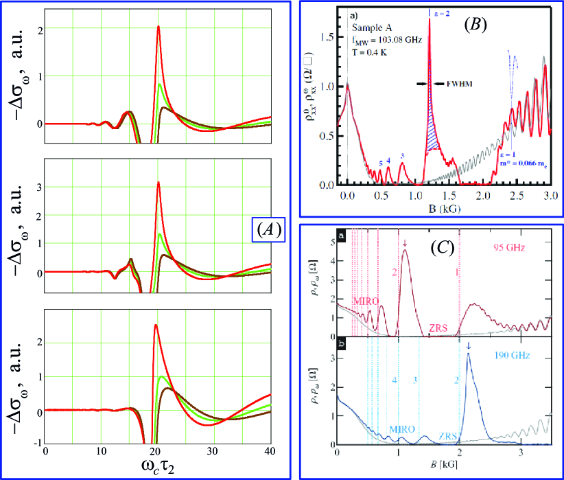
Figure 3: ($A$) Calculated elastic contribution to photoconductivity due to the memory effect in the interparticle energy for Poiseuille flows with the parameters $\omega_{c}\tau_{2}=40$; $\tau_{q}/\tau_{2}=0.5$; $W/L_{s}=4$ (top), $W/L_{s}=1.1$ (middle), $W/L_{s}=0.24$ (bottom). Curves of different colors on each of the subpanels correspond to different relative values of the amplitudes of the contributions to the photoresistance, being proportional to $\cos(2\pi\omega/\omega_{c})$ and $\sin(2\pi\omega/\omega_{c})$ and determined by the values of the coefficients $a,b,c,d$ in Eq. (S27) of SI : $b/a=-0.8$ (red curves), $b/a=-0.28$ (green curves), $b/a=0.08$ (brown curves). Herewith for all curves $c,d=0$. ($B$,$C$) Experimental data Refs. exp_GaAs_ac_1 and exp_GaAs_ac_2 on photoresistance of high-quality GaAs quantum wells for samples where both the giant negative magnetoresistance (thin grey lines), evidencing the hydrodynamic transport regime je_visc , and the $\omega=2\omega_{c}$-peak in photoresistance (red and blue lines) are observed.

In Fig. 3 we compare the calculated elastic contribution to photoconductivity, $\Delta\sigma^{el}_{\omega}$ with the photoresistance measured in GaAs quantum wells of record quality exp_GaAs_ac_1 ; exp_GaAs_ac_2 . In experimental data shown in Fig. 3($B$,$C$) a peak is observed near the doubled cyclotron frequency, $\omega=2\omega_{c}$. It is seen from experimental as well as from theoretical pictures that, depending on the specific parameters of the sample and the electron fluid, the resonance changes its shape and can disappear. In lower magnetic fields, $\omega_{c}<\omega/2$, magnetooscillations appear on both the experimental and theoretical curves. Note that there are no resonance at $\omega=2\omega_{c}$ in the contribution $\Delta\sigma^{rel}_{\omega}$ due to the difference of the $\omega$-dependent amplitudes in $\Delta\sigma^{el}_{\omega}$ and $\Delta\sigma^{rel}_{\omega}$. In this way, the resonance at $\omega=2\omega_{c}$ in photoresistance is another evidence of formation of a highly viscous fluid.

In recent work recentest_ the giant negative magnetoresistance and the peak in photoresistance near $\omega=2\omega_{c}$, similar to the ones presented at Fig. 3, were also observed in high-quality GaAs quantum wells in samples of different geometries. For medium sample widths and at low radiation powers, the irregular shape of MIRO and the $2\omega_{c}$-peak at were seen very well {Fig. 4($b$) in Ref. recentest_ , for details see SI }.

5. Conclusion. We have shown that a flow of a highly viscous 2D electron fluid at microwave radiation in magnetic field exhibits irregular magnetooscillations of photoconductivity and a peak at the doubled cyclotron frequency. These effects are due to the non-linear memory effects in the inter-particle scattering and in the interaction energy of quasiparticles of the Fermi liquid. Observation of such photoconductivity in best-quality GaAs quantum wells evidences that 2D electrons in them form a highly viscous fluid in moderate magnetic fields.

6. Methods. To find photoconductivity, first, one needs to calculate the linear responses $\mathbf{V}_{0}$ and $\mathbf{V}_{1}$ of the fluid on the dc $\mathbf{E}_{0}$ and the ac $\mathbf{E}_{1}(t)$ electric fields. The dc response $\mathbf{V}_{0}=V_{0}\mathbf{e}_{x}$ is a 2D Poiseuille flow with a parabolic profile: $V_{0}(y)=eE_{0}[\,(W/2)^{2}-y^{2}\,]/(2m\eta_{xx})$. Here $\eta_{xx}=(v^{\eta}_{F})^{2}\tau_{2}/4/(1+4\omega_{c}^{2})$ is the dc diagonal viscosity. It depends on magnetic field via the dc diagonal viscosity $\eta_{xx}\sim 1/B^{2}$ je_visc . The linear responses $\mathbf{V}_{1}=V_{1}\mathbf{e}_{x}$ on the ac field of the both polarizations $\mathbf{E}_{1}^{\pm}$ are identical that reflects the screening of $E_{1,y}(t)$. They takes the form vis_res_2 : $V_{1}(y,t)=V_{1}(y)\,e^{-i\omega t}+c.c.$, $V_{1}(y)=ieE_{1}\,[\,1-f_{\lambda}(y)\,]/(2m\omega)$, where $\lambda=\sqrt{-i\omega/\eta_{xx}}$ is the eigenvalue of the transverse magnetosonic waves, $\eta_{xx}=\eta_{xx}(\omega,\omega_{c})\sim$ is the ac diagonal viscosity SI , and $f_{\lambda}(y)=\cosh(\lambda y)/\cosh(\lambda W/2)$. In the viscoelastic regime, $\omega\sim\omega_{c}\gg 1/\tau_{2}$, the imaginary part dominates in $\eta_{xx}$ far from the resonance $\omega=2\omega_{c}$, therefore Navier-Stokes equations (1) turns out into Hooke’s equations. The wavelength and the decay length of the transverse waves at $\omega>2\omega_{c}$ are estimated as $l_{s}=v_{F}^{\eta}/\omega$ and $L_{s}=v_{F}^{\eta}\tau_{2}$ SI . The parameter $v_{F}^{\eta}$ in a strongly non-ideal Fermi liquid is much greater than the Fermi velocity $v_{F}$, thus a flow with characteristic spacescales $l_{s}\gg v_{F}/\omega$ can be described hydrodynamically vis_res_2 ; Semiconductors .

Second, to calculate the small-amplitude photoconductivity proportional the radiation power $\mathcal{W}\sim E_{1}^{2}$ we need the following contributions in the hydrodynamic velocity: $V=V_{0}+V_{1}+V_{\omega}$, where $V_{0}=V_{0}(y)$ and $V_{1}=V_{1}(y,t)$ are the linear responses presented above and $V_{\omega}=V_{\omega}(y)$ is the nonlinear dc component proportional to $E_{0}E_{1}^{2}$. The latter one is calculated in SI on the base of Eqs. (1)-(3) using the perturbation theory by the nonlinear memory inelastic, $\sim\Gamma_{ijkl}$, and elastic, $\delta F_{2,ij}$, terms which depend on the flow characteristics $\Delta_{xy}$, $V$, and $\Pi_{xy}$ corresponding to the linear response $V_{0}+V_{1}$ SI .

Based on the obtained nonlinear dc velocity $V_{\omega}(y)$, we calculate the mean sample photoconductivity by the formula $\Delta\sigma_{\omega}=en_{0}\int_{-W/2}^{W/2}V_{\omega}(y)\,dy/(WE_{0})$. For detail of calculations and for discussion of the results see Supplemental information SI .

7. Acknowledgements. We thank M. I. Dyakonov for numerous discussions of transport experiments on high-mobility electron systems, those led to this work, as well as for discussions of some of the issues raised in this work, for reading the preliminary version of the manuscript, for advice and support. We thank A. P. Dmitriev and Y. M. Beltukov for fruitful discussions. One of us (P. S. A.) thanks E. G. Alekseeva, I. P. Alekseeva, N. S. Averkiev, K. A. Baryshnikov, K. S. Denisov, I. V. Krainov, and S. M. Postolov for advice and support.

This work was financially supported by the Russian Science Foundation (Grant No. 18-72-10111).

Here we present the details of our theoretical model, of the solution of its equations, and of derivation of the properties of the resulting photoconductivity. We discuss possible extensions of our theoretical model to more general hydrodynamic-like systems in disordered samples. We also compare our results with preceding theoretical and experimental works.

S.1 1. Memory effects in scattering of 2D non-interacting electrons on localized defects

Memory effects in classical ac magnetotransport of non-interacting 2D electrons in disordered samples were considered, for example, in Refs. S1 ; S2 ; S3 ; Polyakov_et_al_classical_mem ; S12 ; Beltukov_Dyakonov .

For the scattering of 2D electrons on defects with a localized potential (“impurities”), the memory effects in a perpendicular magnetic field $\mathbf{B}$ are due to the appearance of (i) the electrons not scattering on defects (their trajectories are located between the impurities) and of (ii) the so-called “extended collisions”. The last events consist of several returns of an electron to the same impurity after a first scattering on it because of cyclotron rotation (see Fig. 2 in Ref. Beltukov_Dyakonov ). Both these effects (i) and (ii) become substantial in the classically strong magnetic fields, when the electron mean free path relative to the scattering on defects becomes longer than or comparable with the length of the cyclotron circle S1 ; S12 .

Within the approach of Ref. Beltukov_Dyakonov , such events are accounted in a phenomenological physically transparent way by the retardation term $-\hat{\Gamma}(t)\mathbf{V}(t-T)$ in the Drude-like equation for the mean velocity $\mathbf{V}(t)$:

$$\begin{array}[]{c}\displaystyle\frac{\partial\mathbf{V}}{\partial t}=\frac{e}{m}\,\mathbf{E}(t)+[\,\mathbf{V}\times\bm{\omega_{c}}\,]-\\ \\ \displaystyle\qquad\qquad-(1-P)\,\Big{[}\,\frac{\mathbf{V}}{\tau_{tr}}+\hat{\Gamma}(t)\,\mathbf{V}(t-T)\,\Big{]}\>,\end{array}$$ (S1)

where $e$ and $m$ are the electron charge and the electron mass, the electric field $\mathbf{E}(t)$ can contain dc and ac components; $\bm{\omega_{c}}=\omega_{c}\mathbf{e}_{z}$ is the vector along the magnetic field, $\omega_{c}=eB/(mc)$ is the electron cyclotron frequency, $\tau_{tr}$ is the momentum relaxation time due to the scattering on disorder in the absence of the memory effect,

$$P=e^{-T/\tau_{q}}$$ (S2)

is the probability for an electron to make a full cyclotron rotation without collisions with defects, $\tau_{q}$ is the departure scattering time due to collisions with defects, $T=2\pi/\omega_{c}$ is the cyclotron period, and $\hat{\Gamma}(t)$ is the retarded relaxation tensor due to double extended collisions.

The tensor $\hat{\Gamma}(t)$ depends on the dynamics of individual electrons in the past, $t^{\prime}<t$. At sufficiently weak flows, such dependence is accounted by a nonlinear contributions in $\hat{\Gamma}$ [being additional to the unperturbed value $\hat{\Gamma}^{(0)}$ corresponding to the limit $E,V\to 0$]. This contribution is proportional to the vector $\bm{\Delta}$ characterizing the deviation of the electron trajectories $\mathbf{r}_{0}(t)$ from the exact cyclotron circles:

$$\Gamma_{ij}(\bm{\Delta})=\Gamma_{ij}^{(0)}+\alpha\Delta^{2}\delta_{ij}+\beta\Delta_{i}\Delta_{j}\>.$$ (S3)

Here the coefficients $\hat{\Gamma}^{(0)}$, $\alpha$, and $\beta$ are the microscopic characteristics of the electron gas and the defects, being proportional to the probability $P$ (S2). The vector $\Delta$ for an Ohmic flow is the mismatch $\bm{\Delta}(t)=\bm{\varrho}(t)-\bm{\varrho}(t-T)$ of the impact scattering parameters $\bm{\varrho}(t)=\mathbf{r}_{0}(t)-\mathbf{R}_{0}$ and $\bm{\varrho}(t-T)=\mathbf{r}_{0}(t-T)-\mathbf{R}_{0}$ of an electron in two successive collisions with the same defect [here $\mathbf{R}_{0}$ is the position of the defect center; it follows from the above formulas that $\bm{\Delta}(t)=\mathbf{r}_{0}(t)-\mathbf{r}_{0}(t-T)$]. Such form of relation (S3) of the part of the tensor $\hat{\Gamma}$ related to the perturbation of the trajectories between collisions is valid when the size of defects is small: $a\ll R_{c}$. Provided this inequality, the mismatch $\bm{\Delta}(t)$ is directly related with the forces from the dc and the ac electric fields $\mathbf{E}_{0}$ and $\mathbf{E}_{1}(t)$ acting on an electron during a cyclotron period $t-T<t^{\prime}<t$. Herewith in the approximation linear by $\mathbf{E}_{0}$ and $\mathbf{E}_{1}(t)$, the corresponding value of the mismatch:

$$\bm{\Delta}(t)=\bm{\Delta}_{0}+\bm{\Delta}_{1}(t)\>,$$ (S4)

does not depend on particular parameters of a trajectory $\mathbf{r}_{0}(t)$.

Such model allowed to analytically calculate the photoconductivity of non-interacting 2D electrons in bulk samples Beltukov_Dyakonov . The obtained magnetooscillations of the photoconductivity are induced by the described extended collisions and are similar in many properties to the ones of MIRO observed in experiments.

S.2 2. Memory effects in relaxation due to interparticle scattering in highly viscous 2D electron fluid

Below we formulate and solve phenomenological dynamic equations for the case of 2D interacting electrons forming a highly viscous fluid in samples with no defects (or, more generally, in the sample regions where defects are not substantial for the flow), similar to ones presented in previous section of non-interacting electrons in sample with localized defects.

Our hydrodynamic model accounts the viscosity and the viscoelasticity effects in the ac and the dc components of a flow, respectively, as well as the memory effect in collisions between quasiparticles of the fluid. We will see that such model also leads to magnetooscillations and a peak in photoresistance, coinciding in many properties with MIRO.

For a viscous electron fluid, the motion equation must describe not only of the mean velocity $\mathbf{V}(\mathbf{r},t)$, being now inhomogeneous by $\mathbf{r}$, but also the perturbed electron density $n(\mathbf{r},t)$ and the shear stress tensor $\hat{\Pi}(\mathbf{r},t)$. The hydrodynamic equations of evolution of these values for a highly viscous 2D electron fluid without accounting for the memory effects were formulated and derived in Refs. je_visc ; vis_res_1 ; el ; vis_res_2 ; Semiconductors ; Alekseev_Dmitriev . For the case a high-frequency flow, those equations are transformed into Hooke’s equations of an almost elastic dynamics of an electron media with a weak damping due to the interparticle scattering el ; Semiconductors . In Hooke’s equations, the value that describes the state of the system is the displacement vector $\mathbf{u}(\mathbf{r},t)$, related to the strain tensor $\varepsilon_{ij}(\mathbf{r},t)$. In this work it is convenient to define $\varepsilon_{ij}$ as:

$$\varepsilon_{ij}=\frac{\partial u_{i}}{\partial x_{j}}+\frac{\partial u_{j}}{\partial x_{i}}\>.$$ (S5)

The connection between Hooke’s and the Navier-Stokes equations is based on the following relation for the hydrodynamic velocity in an almost elastic flow of the fluid:

$$\mathbf{V}(\mathbf{r},t)\approx\frac{\partial\mathbf{u}(\mathbf{r},t)}{\partial t}\>.$$ (S6)

This formula describes the absence of slipping between neighbor layers of the flow.

Generally, the dynamics of a viscous fluid with taking into account the interparticle scattering, resulting in slipping between fluid layers, is described by the full set of the hydrodynamic variables: the density $n$, the velocity $\mathbf{V}$, and the shear stress tensor $\Pi_{ij}$ vis_res_1 . Equation (S6) in this case is a formula for calculation, in the linear by $\mathbf{V}$ approximation, of the displacement $\mathbf{u}(\mathbf{r},t)$ of fluid elements. Note that $\mathbf{u}$ for a flow with the slipping of neighbour layers is not the variable sufficient for the description of the fluid dynamics.

Analogously to the dynamics of independent electrons in a sample with small-size defects, the memory effect for an electron fluid in a defectless sample in a magnetic field is due to the “extended collisions” between electron-like Fermi-liquid quasiparticles (see Fig. S1 and Fig. 1 in the main text). Indeed, if the mean free path of quasiparticles relative to their collisions is of the order or larger than the length of the cyclotron circle $2\pi R_{c}$, two quasiparticles can suffer several successive collisions with slow step-like changing of their relative impact scattering parameter $\bm{\varrho}(t)=\mathbf{r}_{0,1}(t)-\mathbf{r}_{0,2}(t)$ (see Fig. S1). This leads to the dependence of the rate of relaxation of the shear stress, $\partial\hat{\Pi}/\partial t$, in the moment $t$ on the characteristic of the fluid in the moments of previous scattering events in the extended collisions, $t-nT$, where $n=1,2,..$ is a number of successive rotations in an extended collision.

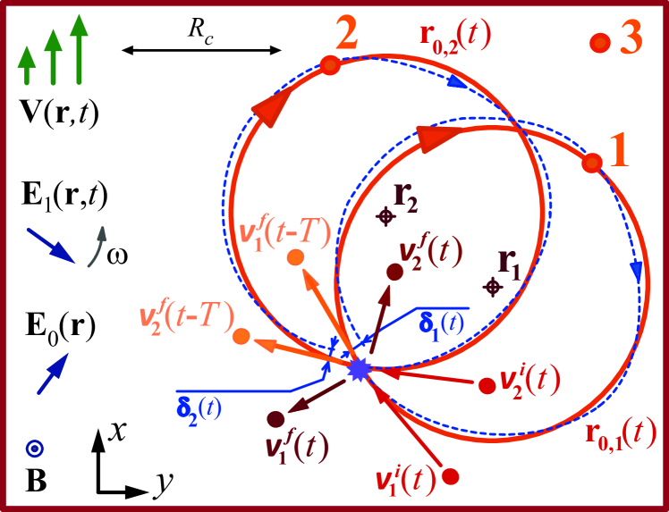
Figure S1: Sketch of the microscopic mechanism of the memory effect in collisions of electron-like quasiparticles in a 2D electron Fermi-liquid in a classical magnetic field $\mathbf{B}=B\mathbf{e}_{z}$. Motion of the fluid, averaged by dynamics of quasiparticles, is described by the hydrodynamic velocity $\mathbf{V}(\mathbf{r},t)$. It contains the components which are linear by the applied electric fields, $\mathbf{V}_{0}(\mathbf{r})\sim\mathbf{E}_{0}$ and $\mathbf{V}_{1}(\mathbf{r},t)\approx\partial\mathbf{u}(\mathbf{r},t)/\partial t\sim\mathbf{E}_{1}(t)$, as well as the nonlinear by $\mathbf{E}_{0}$ and $\mathbf{E}_{1}(t)$ components. Red solid lines are the quasiparticle trajectories at $\mathbf{E}_{0},\mathbf{E}_{1},\mathbf{V}\equiv 0$, which are exact cyclotron circles. Blue dashed lines are the trajectories accounting the elastic force, microscopically related to space-dependent perturbations of the quasiparticle energy spectrum and leading to the term $\sim V_{ij}(\mathbf{r},t)$ in Eq. (S7), as well as to the forces from the full dc and the ac fields $\mathbf{E}_{0}(\mathbf{r},t)$ and $\mathbf{E}_{1}(\mathbf{r},t)$ (S8). The profiles of $\mathbf{V}(\mathbf{r},t)$ and $\mathbf{u}(\mathbf{r},t)$ are changing weakly by $\mathbf{r}$ on the scale of $R_{c}$. The value of the relative impact scattering parameter, $\bm{\varrho}(t^{\prime})=\mathbf{r}_{0,1}(t^{\prime})-\mathbf{r}_{0,2}(t^{\prime})$, at the moment $t^{\prime}=t-T$ differ from its value at $t^{\prime}=t$ on the difference $\bm{\delta}(t)=\bm{\delta}_{1}(t)-\bm{\delta}_{2}(t)$ of the trajectory mismatches by a period: $\bm{\delta}_{p}(t)=\mathbf{r}_{0,p}(t)-\mathbf{r}_{0,p}(t-T)$, $p=1,2$. The values $\bm{\delta}_{p}(t)$ are estimated as the mean shifts of the whole fluid in the centers $\mathbf{r}_{p}$ by a period: $\bm{\delta}_{p}(t)\sim[\mathbf{u}(\mathbf{r}_{p},t)-\mathbf{u}(\mathbf{r}_{p},t-T)]$.

Generally speaking, the reason for the dependence of the fluid relaxation rate at the present moment $t$ on the fluid characteristics at previous moments, $t^{\prime}<t$, consists in a rather long collisionless motion of quasiparticles before moment $t$. Indeed, when describing the motion of a fluid by the distribution function and the corresponding quantities $V(\mathbf{r},t)$ and $\Pi(\mathbf{r},t)$, their average values, used in the theory, are established after last collisions of quasiparticles, that is, at times $t^{\prime}<t$, significantly preceding moment $t$. Accordingly, in the interval $t-nT\lesssim t^{\prime}<t$ the evolution of the fluid is deterministic, which is described by the hydrodynamic motion equations with retarded terms.

The corresponding phenomenological dynamic equations of the fluid, extending the equations from Refs. el ; Semiconductors in order to account the double collisions ($n=1$), can be written in the form:

$$\left\{\begin{array}[]{l}\displaystyle\frac{\partial n}{\partial t}+\tilde{n}_{0}\,\mathrm{div}\mathbf{V}=0\\ \\ \displaystyle\frac{\partial V_{i}}{\partial t}\,=\,\frac{e}{m}\,E_{i}(\mathbf{r},t)+\omega_{c}\epsilon_{ikz}V_{k}-\frac{1}{m}\,\frac{\partial\Pi_{ij}}{\partial x_{j}}\\ \\ \displaystyle\frac{\partial\Pi_{ij}/\partial t}{1\>+\>\delta F_{2,ij}(\mathbf{r},t)/(1+F_{2})}\,=\,2\omega_{c}\,\epsilon_{ikz}\Pi_{kj}\,-\\ \\ \displaystyle-\frac{\Pi_{ij}}{\tau_{2}}-\frac{m(v_{F}^{\eta})^{2}}{4}\,V_{ij}-\Gamma_{ijkl}(\mathbf{r},t)\,\Pi_{kl}(\mathbf{r},t-T)\end{array}\right..$$ (S7)

Here $\tilde{n}_{0}$ is the quasiparticle characteristic being analogous to the equilibrium density $n_{0}=n-\delta n$ in the case of a Fermi gas, but renormalized by the interparticle interaction Semiconductors ; $e$ is the electron charge; $m$ is the electron renormalized mass; the electric field $\mathbf{E}(\mathbf{r},t)$ contains the components from dc and ac external fields induced by the electric bias and the microwave radiation as well as from the internal dc and ac field related to the non-equilibrium charge density $e\,\delta n(\mathbf{r},t)$: $\mathbf{E}(\mathbf{r},t)=\mathbf{E}_{0}(\mathbf{r})+\mathbf{E}_{1}(\mathbf{r},t)$,

$$\begin{array}[]{c}\mathbf{E}_{0}(\mathbf{r})=\mathbf{E}_{0}^{ext}+\mathbf{E}_{0}^{int}(\mathbf{r})\>,\\ \\ \mathbf{E}_{1}(\mathbf{r},t)=\mathbf{E}_{1}^{ext}(t)+\mathbf{E}_{1}^{int}(\mathbf{r},t)\>;\end{array}$$ (S8)

$\epsilon_{ikm}$ is the antisymmetric unit tensor; $V_{ij}=V_{ij}(\mathbf{r},t)$ is the tensor of the gradients of the velocity $\mathbf{V}$:

$$V_{ij}=\frac{\partial V_{i}}{\partial x_{j}}+\frac{\partial V_{j}}{\partial x_{i}}\>;$$ (S9)

$\tau_{2}$ is the shear stress relaxation time without the memory effects; $v^{\eta}_{F}$ is the parameter defining the magnitude of the viscosity $\eta$ of a highly viscous fluid vis_res_2 :

$$\eta|_{B=0}=\,(v_{F}^{\eta})^{2}\,\tau_{2}\,/\,4\>;$$ (S10)

$\hat{\Gamma}_{ijkl}(\mathbf{r},t)$ is the tensor describing the retarded relaxation of $\Pi_{ij}$ due to the extended collisions (see Fig. S1); $T=2\pi/\omega_{c}$ is the cyclotron period; and $\delta F_{2,ij}(\mathbf{r},t)$ are the perturbations of the coefficient $F_{2}$ of the Landau function. The values $\delta F_{2,ij}$ describe the effect of the viscous motion on the quasiparticle energy spectrum.

Below in this section we discuss the inelastic contribution to the memory effect in Eqs. (S7), described by the term $\hat{\Gamma}_{ijkl}(\mathbf{r},t)\,\Pi_{kl}(\mathbf{r},t-T)$. The elastic contribution to the memory effect, $\sim\delta F_{2,ij}(\mathbf{r},t)$, will be studied in the next section.

In view of a phenomenological character of the theory, we have not presented in Eq. (S7) the Fermi-liquid renormalizations of all the parameters in an exact form. These renormalizations were studied in Ref. Semiconductors and are important for the quantitative calculations. So further we will consider that $\tilde{n}_{0}=n_{0}$, $F_{1}=0$, $F_{2}=0$.

In the latter equation of system (S7) we also omit the factor $(1-P)\sim 1$ for simplicity [compare Eqs. (S1) and (S7). In the hydrodynamic equations the value

$$P=e^{-T/\tau_{q}}\>,$$ (S11)

is the probability to make a full cyclotron rotation for a quasiparticle in a pair without collisions with other quasiparticles. The time $\tau_{q}$ in $P$ is the departure scattering time relative to interparticle collisions.

We consider that the characteristic radius $a$ of the interparticle interaction potential is much smaller than the cyclotron radius. In this case, each extended collision consists of two (or several) successive collisions of two quasiparticles in a small region (a blue star in Fig. S1) and of almost collisionless motions of these two quasiparticles far from the region of scattering. This motion is mainly determined by the magnetic field, but is also substantially affected by the full electric field $\mathbf{E}(\mathbf{r},t)$ (S8) as well as by the elastic force, related to the space-dependent change of the quasiparticle energy spectrum el ; Semiconductors and leading to the term $\sim V_{ij}(\mathbf{r},t)$ in Eq. (S7). The elastic force and the components $\mathbf{E}_{0}^{int}$ and $\mathbf{E}_{1}^{int}$ of field (S8) are inhomogeneous by $\mathbf{r}$ and are determined by the formation of the flow in the whole sample. These inhomogeneities lead to the difference of the full forces acting on two quasiparticles “1” and “2” (see Fig. S1). This difference defines the dependence of the probability of the extend collisions on the flow magnitude and shape in the current moment and in the past. For example, the probability to return to the same place for two quasiparticles is much greater for a stationary homogeneous flow than for a fast ac flow, in which the memory about positions of two quasiparticles can be lost with a large probability in one cyclotron rotation (see Fig. S1).

To describe such memory effect microscopically, one should use the Boltzmann-like kinetic equation with a generalized collision operator of the inter-quasiparticle scattering, being nonlocal by time. Such collision operator, leading to the motion equation of the type of Eqs. (S7), could be derived within some sophisticated procedure from the classical or the quantum Liuville equations for the interacting Fermi-liquid electron-like quasiparticles. Herewith some other retarded terms in the resulting effective transport equations, except the term $-\Gamma_{ijkl}(\mathbf{r},t)\Pi_{kl}(\mathbf{r},t-T)$ accounted in Eq. (S7), may be possible, for example: $A_{ij}E_{j}(\mathbf{r},t-T)$, $B_{ijkl}E_{j}(\mathbf{r},t-T)\Pi_{kl}(\mathbf{r},t-T)$, and so on S4 . However we hope that the term $-\Gamma_{ijkl}(\mathbf{r},t)\Pi_{kl}(\mathbf{r},t-T)$ is sufficient to describe the main properties of the photoconductivity induced by the memory effect in interparticle collisions.

Quantitatively, the extended inter-particle collisions are characterized by the following values. Two successive collisions are controlled by the impact relative scattering parameter of particles “1” and “2” (see Fig. S1):

$$\bm{\varrho}(t^{\prime})=\mathbf{r}_{0,1}(t^{\prime})-\mathbf{r}_{0,2}(t^{\prime})\>,\quad t^{\prime}=t,\;t-T\>.$$ (S12)

During one cyclotron period $t-T<t^{\prime}<t$, two scattered quasiparticles are moving along the trajectories $\mathbf{r}_{0,1}(t)$ and $\mathbf{r}_{0,2}(t)$ with the centers near the points $\mathbf{r}_{1}$ and $\mathbf{r}_{2}$. Their impact scattering parameter $\bm{\varrho}(t^{\prime})$ (S12) differs in the moments $t^{\prime}=t$ and $t^{\prime}=t-T$ on the value $\bm{\delta}(t)=\bm{\delta}_{1}(t)-\bm{\delta}_{2}(t)$, where $\bm{\delta}_{1}(t)$ and $\bm{\delta}_{2}(t)$ are the mismatches of the trajectories $\mathbf{r}_{0,1}(t)$ and $\mathbf{r}_{0,2}(t)$ by a cyclotron period:

$$\begin{array}[]{c}\displaystyle\bm{\delta}(t)=\bm{\varrho}(t)-\bm{\varrho}(t-T)=\bm{\delta}_{1}(t)-\bm{\delta}_{2}(t)\>,\\ \\ \bm{\delta}_{p}(t)=\mathbf{r}_{0,p}(t)-\mathbf{r}_{0,p}(t-T)\,,\quad p=1,2\,.\end{array}$$ (S13)

Nonzero values of the mismatches $\bm{\delta}_{p}(t)$ are induced by the action of the elastic force $V_{ij}(\mathbf{r},t)$ and the electric fields (S8), as it was discussed above (see also Fig. S1).

In accordance with the essence of the extended collisions, the tensor $\Gamma_{ijkl}(\mathbf{r},t)$ in the retarded relaxation term in Eq. (S7) is determined by the mismatches $\bm{\delta}(t)$ (S13) of the scattering parameters $\bm{\varrho}(t^{\prime})$ (S12), averaged by all the quasiparticle pairs near the given point $\mathbf{\mathbf{r}}$. The averaged mismatch $\langle\bm{\delta}(t)\rangle$ is apparently expressed via the macroscopic variables of the fluid in the past, generally speaking, via all variables: $n$, $\mathbf{V}$, $\hat{\Pi}$. Thus the tensor $\Gamma_{ijkl}(\mathbf{r},t)$ depends on these variables as an operator:

$$\Gamma_{ijkl}(\mathbf{r},t)=\hat{\Gamma}_{ijkl}[n(\mathbf{r}^{\prime},t^{\prime}),\mathbf{V}(\mathbf{r}^{\prime},t^{\prime}),\hat{\Pi}(\mathbf{r}^{\prime},t^{\prime})]\>,$$ (S14)

where $|\mathbf{r}-\mathbf{r}^{\prime}|\lesssim R_{c}$ and $t-T\lesssim t^{\prime}<t$.

We consider high-frequency regime when that interparticle are rare as compared with cyclotron period: $\omega,\omega_{c}\gg 1/\tau_{2}$. In this case, a collision of one of two particles during an extended collision with a third particle is a rare event, thus $P\sim 1$ (see Fig. S1). Thus the only macroscopic variable determining the mismatches $\bm{\delta}_{1}(t)$ and $\bm{\delta}_{2}(t)$ is the displacement vector $\mathbf{u}(\mathbf{r}^{\prime},t^{\prime})$ in the centers of the particle trajectories “1” and “2” (see Fig. S1):

$$\bm{\delta}_{p}(t)\sim\mathbf{u}(\mathbf{r}_{p},t)-\mathbf{u}(\mathbf{r}_{p},t-T)\>,\quad p=1,2\>.$$ (S15)

For the resulting dependence of $\hat{\Gamma}$ on the shape and the magnitude of the flow we have:

$$\begin{array}[]{c}\hat{\Gamma}_{ijkl}[\mathbf{u}(\mathbf{r}^{\prime},t^{\prime})]=\Gamma_{ijkl}\Big{(}\big{\langle}\,\bm{\delta u}(\mathbf{r}_{1},\mathbf{r}_{2},t)\,\big{\rangle}_{\mathbf{r}_{1},\mathbf{r}_{2}}\Big{)}\end{array}\>,$$ (S16)

where the brackets $\langle\,.\,\rangle_{\mathbf{r}_{1},\mathbf{r}_{2}}$ denote the averaging by $|\mathbf{r}-\mathbf{r}_{p}|\lesssim R_{c}$, $p=1,2$, and the vector $\bm{\delta u}$ is:

$$\begin{array}[]{c}\bm{\delta u}(\mathbf{r}_{1},\mathbf{r}_{2},t)=[\mathbf{u}(\mathbf{r}_{1},t)-\mathbf{u}(\mathbf{r}_{1},t-T)]-\\ \\ -[\mathbf{u}(\mathbf{r}_{2},t)-\mathbf{u}(\mathbf{r}_{2},t-T)]\end{array}\>.$$ (S17)

Here the displacement $\mathbf{u}(\mathbf{r},t)$ can consist of the ac near-elastic as well as the dc dissipative parts, both related to the ac and dc components of $\mathbf{V}(\mathbf{r},t)$ by Eq. (S6).

In the hydrodynamic regime, the characteristic spacescale of the inhomogeneity of the flow, $W$, is much larger than $R_{c}$, therefore we have:

$$u_{m}(\mathbf{r}_{1},t^{\prime})-u_{m}(\mathbf{r}_{2},t^{\prime})\approx(x_{1n}-x_{2n})\,\frac{\partial u_{m}(\mathbf{r}_{1},t^{\prime})}{\partial x_{n}}\>,$$ (S18)

where the summation by $n$ is supposed. Thus the expression $\bm{\delta u}(\mathbf{r}_{1},\mathbf{r}_{2},t)$ (S17), averaged by $\mathbf{r}_{1}$ and $\mathbf{r}_{2}$, is expressed via the shift (the “mismatch”) $\Delta_{mn}(\mathbf{r},t)$ of the strain tensor $\varepsilon_{mn}(\mathbf{r},t)$ in a cyclotron period. For the resulting $\hat{\Gamma}$ we obtain:

$$\begin{array}[]{c}\hat{\Gamma}_{ijkl}[\,\mathbf{u}(\mathbf{r}^{\prime},t^{\prime})\,](\mathbf{r},t)=\Gamma_{ijkl}\big{(}\,\Delta_{mn}(\mathbf{r},t)\,\big{)}\,,\\ \\ \Delta_{mn}(\mathbf{r},t)=\varepsilon_{mn}(\mathbf{r},t)-\varepsilon_{mn}(\mathbf{r},t-T)\>.\end{array}$$ (S19)

Expansion of $\Gamma_{ijkl}$ by $\Delta_{mn}$ up to the quadratic order is:

$$\begin{array}[]{c}\displaystyle\Gamma_{ijkl}(\Delta_{mn})=\Gamma^{(0)}_{ijkl}\,+\,\alpha^{mnop}_{ijkl}\,\Delta_{mn}\,\Delta_{op}\>,\end{array}$$ (S20)

where the tensors $\Gamma^{(0)}_{ijkl}$ and $\alpha^{mnop}_{ijkl}$ are determined by the parameters of the fluid and depend on temperature and magnetic field. The linear term $a^{mn}_{ijkl}\,\Delta_{mn}$ is absent in Eq. (S20) due to the symmetry of the relaxation processes relative to the inversion of the direction of flows.

From Eq. (S6) we obtain the expression for the mismatch of the strain tensor via the velocity gradient $V_{mn}(\mathbf{r},t^{\prime})$:

$$\Delta_{mn}(\mathbf{r},t)\approx\int_{t-T}^{t}dt^{\prime}\;V_{mn}(\mathbf{r},t^{\prime}\,)\>.$$ (S21)

Here, similarly to Eqs. (S8), the tensor $V_{mn}$ can contain both the ac component corresponding to an almost elastic dynamics and the dc component corresponding to a dissipative viscous motion.

One should expect that the tensors $\Gamma^{(0)}_{ijkl}$ and $\alpha^{mnop}_{ijkl}$ are proportional to the probability $P$ (S11) [or, possibly, $P^{2}$] to make a full rotation for a quasiparticles in a pair without collisions with other quasiparticles and to some interparticle scattering rate, apparently, the rate of the relaxation of the shear stress $1/\tau_{2}$

According to Fig. S1, the relative value of the correction to the probability of an extended collision from the deviation of the trajectories $\mathbf{r}_{0,p}(t)$ from exact cyclotron circles is proportional to the squared ratio $|\bm{\delta}(t)|/a_{B}$. Here the value

$$|\bm{\delta}(t)|\sim||\hat{\Delta}(\mathbf{r},t)||\,R_{c}$$ (S22)

is the characteristic difference of the mismatches of the trajectories of quasiparticles near the point $\mathbf{r}$ at the moment $t$ and $a_{B}$ is the Bohr radius, being the estimate for the size of the interparticle interaction potential. In this way, according to the definition of the tensors $\Gamma^{(0)}_{ijkl}$ and $\alpha^{mnop}_{ijkl}$ in Eq. (S20), we have:

$$\begin{array}[]{c}\displaystyle\Gamma^{(0)}_{ijkl}=\,A_{ijkl}\>\frac{e^{-T/\tau_{q}}}{\tau_{2}}\>,\\ \\ \displaystyle\alpha^{mnop}_{ijkl}=\,B^{mnop}_{ijkl}\>\Big{(}\,\frac{\displaystyle R_{c}}{\displaystyle a_{B}}\,\Big{)}^{2}\>\frac{e^{-T/\tau_{q}}}{\tau_{2}}\>,\end{array}$$ (S23)

where $A_{ijkl}$ and $B^{mnop}_{ijkl}$ are the numeric constants independent on the fluid parameters. We remind that for the case of the electron scattering on soft impurities, analogous formulas for the memory constants $\alpha$ and $\beta$ in the tensor (S3) were derived in Ref. Beltukov_Dyakonov and lead to the estimations of $\alpha$ and $\beta$ analogous to Eq. (S23).

Formulas (S23) lead to a definite dependence of the retarded relaxation terms on the magnetic field (via $T$ and $R_{c}$) and on the temperature $T_{e}$ of the electron fluid via the times $\tau_{2}$ and $\tau_{q}$. The departure time $\tau_{q}$ is usually somewhat smaller than the stress relaxation time $\tau_{2}$, but they has similar temperature dependencies for 2D degenerate electrons at any strength of interparticle interaction Novikov ; Alekseev_Dmitriev . Up to the logarithmic factor $\ln(\varepsilon_{F}/T_{e})$, being weakly dependent on the temperature $T_{e}$, both the rates $1/\tau_{q}$ and $1/\tau_{2}$ are the quadratic functions of $T_{e}$ Novikov ; Alekseev_Dmitriev :

$$\frac{\hbar}{\tau_{q,2}}=C_{q,2}(T)\,\frac{T_{e}^{2}}{\varepsilon_{F}}\>.$$ (S24)

Here $\varepsilon_{F}$ is the Fermi energy of the electron fluid and $C_{q,2}(T_{e})$ are the dimensionless coefficients, which are determined by the interparticle interaction parameter $r_{s}$, related to the electron density $n_{0}$, and can weakly depend on temperature via the logarithm $\ln(\varepsilon_{F}/T_{e})$.

S.3 3. Memory effects in elastic part of interparticle interaction in highly viscous 2D electron fluid

The memory effect due to the formation of pairs of quasiparticles can also lead to non-dissipative “elastic” retarded terms in the viscoelastic motion equation. Microscopically, elastic retarded terms are related to a collisionless motion of quasiparticles in a pair during several cyclotron periods, a formation of a statistical distribution of quasiparticles before the current moment (after collisions preceding the collisionless motion of pairs), and the dependence of energy of the pairs of quasiparticles on the external electric and stress fields during the previous collisions (see Fig. S2).

In this section, we develop a phenomenological description of this effect related to the appearance of the extended collisions within the Drude-like equations of the viscous transport by Eqs. (S7). Namely, we qualitatively construct the form of the corrections $\delta F_{2,ij}(\mathbf{r},t)=\delta F_{2,ij}[\mathbf{V}(\mathbf{r}^{\prime},t^{\prime})]$ to the Landau parameter $F_{2}$ entering Eqs. (S7).

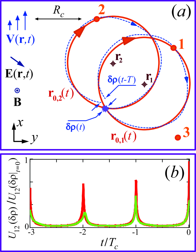
Figure S2: ($a$): A pair of quasiparticles 1 and 2 in a highly viscous electron fluid in magnetic field, undergoing an extended collision. Red curves are cyclotron circles corresponding to the absence of macroscopic fluid motion, while the blue dashed curves take into account the effect of a finite inhomogeneous velocity of the fluid flow on the quasiparticle trajectory. ($b$): Energy of the interaction of the quasiparticles 1 and 2 in the pair shown in panel ($a$) (schematically). This function has maximums at the time moments $t=t-mT$, when the distance between the quasiparticles is of the order of the interaction radius. Red and green curves correspond to smaller and larger amplitudes of the inhomogeneous hydrodynamic velocity $\mathbf{V}(\mathbf{r},t)$, leading to larger and smaller values perturbations of distance between particles $\delta\varrho(t)=|\mathbf{r}_{0,1}(t)-\mathbf{r}_{0,2}(t)|$ and, thus, their interaction energy $U_{12}(\delta\varrho)$.

The energy of the interparticle interaction in a fluid and the resulting elastic forces depend on correlations in the mutual arrangement and velocities of quasiparticles. In classical magnetic fields, correlations between the positions of particles evolve in time according to laws that take into account cyclotron rotation, approach and removal of particles those control the interaction forces, and the Fermi-liquid many-particle effects. At each moment of time, the energy of the interparticle interaction is determined primarily by the quasiparticles located at minimal distances from each other. Two such quasiparticles are shown in Fig. S2(a). At the moments of time $t^{\prime}=t-nT$ they undergo “extended” collisions, that is they approach each other at distances of the order of the radius of their interaction. If during one period many pairs of quasiparticles did not destroyed due to collisions with a third quasiparticle, their configuration one or several cyclotron revolutions ago, $t^{\prime}=t-nT$, was similar to the configuration at moment $t$. So the interaction energy of quasiparticles, which describes the effect of the distribution of quasiparticles on their energy spectrum through the Landau function, depends mainly on the distribution function of quasiparticles at the moments $t$ and $t^{\prime}=t-nT$, when the quasiparticles, the correlation between which is important at $t$, also had especially closely approached one to another.

To illustrate such a mechanism of the dependence of the elastic part of the interaction between quasiparticles on the motion of the fluid due to the formation of pairs, in Fig. S2(b) we have schematically drawn the dependence of the energy of the screened Coulomb interaction of two charged quasiparticles in a pair on time [Fig. S2(b)]. The plotted value $U_{12}(t)$ determines the characteristic scales of the perturbation of the Landau function due to the influence of a fluid motion on the correlations in the dynamics of the most important pairs.

Within our phenomenological theory, we account the perturbation of the elastic part of interparticle interaction only by a nonlocal in time perturbation of the second harmonic of the Landau function $F_{2}$. For a flow in a long sample shown in Fig.1(a) we write:

$$\delta F_{2,xx/xy}=\delta F_{2,xx/xy}^{(0)}+\delta F_{2,xx/xy}^{(1)}\>,$$ (S25)

where the values $\delta F_{2,xx/xy}^{(0)}(y,t)\ll F_{2}$ depend on the values $V(y,t)$, $\Pi_{xx}(y,t)$, $\Pi_{xx}(y,t)$, while the values $\delta F_{2,xx/xy}^{(1)}(y,t)\ll F_{2}$ are expressed via $V(y,t-T)$, $\Pi_{xx}(y,t-T)$, $\Pi_{xx}(y,t-T)$. Perturbations of the harmonic $F_{1}$, apparently, can be neglected, since $F_{1}$ is responsible for the equilibrium properties of the fluid: the renormalization of the quasiparticle mass, the zero and ordinary sound dispersions. The difference between the $xx$- and $xy$-components of the corrections in $F_{2}$ is due to the fact that a nonzero shear stress causes a breaking of the symmetry of the Fermi surface with respect to the quasiparticle velocity angle $\varphi$, therefore the Landau function $F(\varphi)$ becomes asymmetric in $\varphi$. To account only the retardation effect, we will further keep only the contribution $\delta F_{2,xx/xy}^{(1)}$.

The power of thermal energy dissipated at a given point of the viscous fluid flow is:

$$\mathcal{W}=-\,V_{ik}\,\Pi_{ik}\,/\,2\>,$$ (S26)

where summation over same indices is meant. Similarly, in a viscous inhomogeneous flow the relationship between the total energy of the fluid and the inhomogeneous part of the distribution function of quasiparticles, $\delta f_{\mathbf{p}}$, are perturbed. Thus the spectrum of quasiparticles and the Landau parameters describing the fluid energy at $\delta f_{\mathbf{p}}\neq 0$ acquire correction proportional to powers of $\delta f_{\mathbf{p}}$, $V_{ik}$, and $\Pi_{ik}$.

By analogy with Eq. (S26), for the perturbation of the second harmonic of the Landau function $F_{2}$ in the Poiseuille flow, in which only the derivative $\partial V_{x}/\partial y$ is nonzero, we write:

$$\begin{array}[]{c}\displaystyle\delta F_{2,xx}^{(1)}(y,t)=\Big{[}(\,a\>\Pi_{xx}+b\>\Pi_{xy}\,)\,\frac{\partial V}{\partial y}\Big{]}\,\Big{|}_{t^{\prime}=t-T}\,,\\ \\ \displaystyle\delta F_{2,xy}^{(1)}(y,t)=\Big{[}(\,c\>\Pi_{xx}+d\>\Pi_{xy}\,)\,\frac{\partial V}{\partial y}\Big{]}\,\Big{|}_{t^{\prime}=t-T}\,.\end{array}$$ (S27)

Apparently, all coefficients $a,b,c,d$ in this formula are nonzero due to the tensor nature of the perturbations $\delta F_{2,xx/xy}$ and the presence of magnetic field leading to non-diagonal kinetic coefficients. Within the proposed mechanism of the perturbation of the elastic part of the interparticle interaction due to formation of pairs, the coefficients $a,b,c,d$ are to be proportional to the probability for a quasiparticle to make a complete cyclotron circle without collisions with a third quasiparticle: $a,b,c,d\sim e^{-T/\tau_{q}}$.

In this way, we formulated a closed system of equations, Eqs. (S7), (S19)-(S21), and (S27), describing the dynamics of the highly viscous 2D electron fluid in a magnetic field with takin into account the memory effects in the interparticle scattering and in the interparticle interaction energy.

S.4 4. Linear responses of highly viscous electron fluid
on dc and ac electric fields

In order to study the photoresistance effect within the proposed model, first of all, we need to find the linear responses of the fluid on a dc and an ac electric fields $\mathbf{E}_{0}$ and $\mathbf{E}_{1}(t)$.

Both these fields can be written as $\mathbf{E}(t)=\mathbf{E}(\omega)\,e^{-i\omega t}+c.c.$ with $\omega=0$ and $\omega\neq 0$. The linear responses should be calculated by linearized equations (S7) applied to the $\omega$ harmonics of the hydrodynamic velocity $\mathbf{V}(\mathbf{r},t)=\mathbf{V}(\mathbf{r},\omega)e^{-i\omega t}+c.c.$, the density perturbation $\delta n(\mathbf{r},t)=\delta n(\mathbf{r},\omega)e^{-i\omega t}+c.c.$, and the shear stress tensor $\hat{\Pi}(\mathbf{r},t)=\hat{\Pi}(\mathbf{r},\omega)e^{-i\omega t}+c.c.$, corresponding to the harmonics of $\mathbf{E}(t)$.

First, we formulate the resulting equations for the amplitudes $\mathbf{V}(\mathbf{r},\omega)\sim\hat{\Pi}(\mathbf{r},\omega)\sim\mathbf{E}(\omega)$ at a general geometry of a flow.

A solution of the last of equations (S7) without the memory effect term $-\Gamma_{iklm}(\mathbf{r},t)\Pi_{lm}(\mathbf{r},t-T)$ leads to the following linear relation between the time harmonics of the momentum flux $\Pi_{ij}=\Pi_{ij}(\mathbf{r},\omega)$ and of the gradients of the harmonics of the velocity $V_{ij}(\mathbf{r},\omega)=\partial V_{i}/\partial x_{j}+\partial V_{j}/\partial x_{i}$ vis_res_1 :

$$\Pi_{ij}=m\,[\,\eta_{xx}(\omega)\,V_{ij}+\epsilon_{ikz}\eta_{xy}(\omega)\,V_{kj}\,]\>,$$ (S28)

where the ac viscosity coefficients $\eta_{xx}=\eta_{xx}(\omega)$ and $\eta_{xy}=\eta_{xy}(\omega)$ have the form vis_res_1 :

$$\begin{array}[]{c}\eta_{xx}\\ \eta_{xy}\end{array}\Big{\}}=\frac{(v^{\eta}_{F})^{2}\tau_{2}/4}{1+(4\omega_{c}^{2}-\omega^{2})\tau_{2}^{2}-2i\omega\tau_{2}}\,\Big{\{}\begin{array}[]{c}1-i\omega\tau_{2}\\ 2\omega_{c}\tau_{2}\end{array}.$$ (S29)

The second of equations (S7) with $\hat{\Pi}(\mathbf{r},\omega)$ from Eq. (S28) is transformed into the Naiver-Stokes equation for the harmonic of the velocity $\mathbf{V}=\mathbf{V}(\mathbf{r},\omega)$:

$$\begin{array}[]{c}\displaystyle-i\omega\mathbf{V}=\frac{e}{m}\,\mathbf{E}(\omega)+[\,\mathbf{V}\times\bm{\omega}_{c}\,]+\\ \\ \displaystyle+\,\eta_{xx}(\omega)\>\Delta_{L}\mathbf{V}+\,\eta_{xy}(\omega)\>\Delta_{L}\mathbf{V}\times\mathbf{e}_{z}\>,\end{array}$$ (S30)

where $\Delta_{L}=\partial^{2}/\partial x^{2}+\partial^{2}/\partial y^{2}$ is the Laplace operator.

The role of the retarded relaxation term in the last of equations (S7) for the linear response is as follows. If we choose the main part $\hat{\Gamma}^{(0)}$ of the relaxation tensor $\hat{\Gamma}(\mathbf{r},t)$ in the simplest form:

$$\Gamma_{ijkl}^{(0)}=\delta_{ik}\delta_{jl}\,\frac{1}{\tau_{2}^{\prime}}\>,$$ (S31)

we arrive to a redefinition of the relaxation rate $1/\tau_{2}$ which enters Eq. (S29) as compared with its value in the absence of the memory effects:

$$\frac{1}{\tau_{2}}\,\to\,\frac{1}{\tau_{2}}\,+\,\frac{e^{2\pi i\omega/\omega_{c}}}{\tau_{2}^{\prime}}\>.$$ (S32)

For the time $\tau_{2}^{\prime}$ here we should use estimate (S23): $1/\tau_{2}^{\prime}\sim e^{-T/\tau_{q}}/\tau_{2}$.

Further in this work we do not take into account redefinition (S32) of $\tau_{2}$ by the two reasons. First, in view of estimate (S23), the second term in this formula is much smaller than the first one on the factor $e^{-T/\tau_{q}}$, which is substantially smaller than unity at $\omega_{c}\sim\omega\gg 1/\tau_{2},1/\tau_{q}$. Second, our analysis shows that redefinition (S32) leads only to some subtle distortion of the sinusoidal dependence of a factor in the resulting photoconductivity on the ratio $\omega/\omega_{c}$. For the current work, being a first proposal of the hydrodynamic mechanism of MIRO, such detail is not substantial.

We remind that the parameter $v^{\eta}_{F}$ in Eq. (S29) for a strongly non-ideal electron Fermi liquid with large Landau parameters, $F_{m}\gg 1$, is much greater than the actual Fermi velocity $v_{F}$ vis_res_2 ; Semiconductors .

Second, we use equations (S29) and (S30) to calculate the the linear response of the electron fluid on the applied dc and the ac fields, $\mathbf{E}_{0}$ and $\mathbf{E}_{1}(t)$, in a Poiseuille-flow like geometry: a long straight sample with rough edges [see Fig. 1(a) in the main text]. We consider that the sample width $W$ is much smaller than the characteristic plasmon wavelength $l_{p}$:

$$W\ll l_{p}\>,\qquad l_{p}=s/\omega\>.$$ (S33)

Here we use the estimate of $l_{p}$ for a quantum well with a metallic gate. The value $s$ is the plasmon velocity in such structure which is usually much larger than $v_{F}$ and $v_{F}^{\eta}$. In defectless samples of such widths the dc and ac linear responses are formed mainly by a dissipative viscous flow and by standing magnetosonic waves, respectively, whereas the plasmonic contribution to the ac flow component is suppressed to the extent of the small parameter $v_{F}^{\eta}/s\ll 1$ vis_res_2 .

In such flow geometry, only the $x$ component of the velocity $\mathbf{V}$ and the $xy$ component of the velocity gradient tensor $V_{ij}$ are substantial in both the ac and dc components vis_res_2 . For the ac flow component, the density perturbation $\delta n(y,t)$ and the $y$ component of the velocity $V_{y,1}(y,t)$ are relatively small quantities being proportional to $(v_{F}^{\eta}/s)^{2}\ll 1$ vis_res_2 . However, such $\delta n$ determines the not small ac component $E^{int}_{y,1}(y,t)$ of the internal Hall field, which screens the $y$ component of the radiation fields $E_{y,1}(t)$ [see Eqs. (S8)]. For the dc flow component, $V_{y,0}\equiv 0$ and the density perturbation $\delta n(y)$ determines the dc part of the Hall field $E^{int}_{y,0}(y)$.

Thus, in order to find the velocity $\mathbf{V}=\mathbf{V}_{0}+\mathbf{V}_{1}$ we need only the $x$-component of equation (S30). For each component $\mathbf{V}_{0}$ and $\mathbf{V}_{1}$ it takes the form:

$$-i\omega V=\frac{e}{m}\,E_{x}(\omega)+\,\eta_{xx}(\omega)\>\frac{d^{2}V}{dy^{2}}\>.$$ (S34)

The both fields $E^{int}_{y,0}(y)$ and $E^{int}_{y,1}(y,t)$ are calculated from the $y$-components of equation (S30) je_visc .

The resulting response of the fluid in such sample on a dc electric field $\mathbf{E}_{0}^{ext}=E_{0}\mathbf{e}_{x}$ is the dc Poiseuille flow with a parabolic profile. From Eq. (S34) at zero frequency, $\omega=0$, with the diffusive boundary conditions:

$$V\big{|}_{y=\pm W/2}=0\>,$$ (S35)

we obtain for the dc component $V_{0}$ of the velocity $V$ je_visc :

$$V_{0}(y)=\frac{eE_{0}}{2m\eta_{xx}}\,\Big{[}\Big{(}\frac{W}{2}\Big{)}^{2}-y^{2}\,\Big{]}\>,$$ (S36)

where the dc diagonal viscosity coefficient is:

$$\eta_{xx}=\eta_{xx}(0)=\frac{(v_{F}^{\eta})^{2}\tau_{2}/4}{1+4\omega_{2}\tau_{2}^{2}}\>.$$ (S37)

The corresponding averaged sample conductivity:

$$\sigma_{0}=\frac{I_{0}}{E_{0}W}\,,\quad\;\;I_{0}=en_{0}\int_{-W/2}^{W/2}dy\,V_{0}(y)\>,$$ (S38)

and the averaged resistivity $\varrho_{0}=1/\sigma_{0}$ strongly depend on a magnetic field via the viscosity coefficient $\eta_{xx}$.

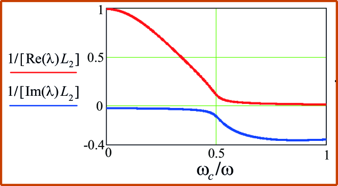
Figure S3: Reciprocal real and imaginary parts of the eigenvalue $\lambda$, describing the decay length and the wavelength of the transverse magnetosonic waves. Thes values are plotted as functions of the ratio $\omega_{c}/\omega\sim B$ at a high ac frequency, $\omega\tau_{2}=20$.

Next, we calculate the linear response of the fluid in the same long sample on the left and the right ac circularly polarized radiation fields:

$$\mathbf{E}^{ext}(t)=\mathbf{E}_{1}^{\pm}e^{-i\omega t}+c.c.\>,\quad\mathbf{E}_{1}^{\pm}=\frac{E_{1}}{2}\left(\begin{array}[]{c}1\\ \pm i\end{array}\right)\>.$$ (S39)

As in was mentioned above, at condition (S33) the response $\mathbf{V}_{1}=V_{1}\mathbf{e}_{x}$ is mainly formed by the transverse magnetosonic waves. According to Eq. (S34), the resulting velocity is almost independent on the sign “$\pm$” of the circular polarization of field (S39): $V^{\pm}_{1}(y,t)\approx V_{1}(y,t)$. From Eq. (S34) with the boundary condition (S35) we obtain $V_{1}(y,t)=V_{1}(y)\,e^{-i\omega t}+c.c.$, where:

$$V_{1}(y)=\frac{eE_{1}}{2m}\,\frac{i}{\omega}\,\Big{[}\,1-\frac{\cosh(\lambda y)}{\cosh(\lambda W/2)}\,\Big{]}\>,$$ (S40)

and $\lambda=\lambda(\omega,\omega_{c})$ is the eigenvalue corresponding to the transversal magnetosonic waves. It is seen from Eq. (S34) that:

$$\lambda=\sqrt{\frac{-i\,\omega\>\;}{\eta_{xx}(\omega)}}\>\;.$$ (S41)

The reciprocal imaginary and real parts of this eigenvalue, $1/\mathrm{Im}\,\lambda$ and $1/\mathrm{Re}\,\lambda$, provide the wavelength and the decay length of the magnetosonic waves, respectively. Their dependencies on $\omega_{c}$ at a fixed frequency $\omega\gg 1/\tau_{2}$ are drawn in Fig. S3.

Far above from the viscoelastic resonance ($\omega-2\omega_{c}\gg 1/\tau_{2}$) we obtain from Ref. (S41) the following estimates for the length of decay and the wavelength of magnetosonic waves:

$$\frac{1}{\mathrm{Re}\,\lambda}\sim L_{s}=v^{\eta}_{F}\tau_{2}\>,\quad\quad\frac{1}{\mathrm{Im}\,\lambda}\sim l_{s}=\frac{v_{F}^{\eta}}{\omega}\>,$$ (S42)

which lead to the relation $1/\mathrm{Re}\lambda\gg 1/\mathrm{Im}\lambda$. Thus, in this regime the solution $V_{1}(y,t)\sim e^{-i\omega t+\lambda y}$ is well-formed weakly decaying waves.

Far below the viscoelastic resonance ($2\omega_{c}-\omega\gg 1/\tau_{2}$), visa versa, we have:

$$\frac{1}{\mathrm{Re}\,\lambda}\sim l_{s}\,,\qquad\frac{1}{\mathrm{Im}\,\lambda}\sim L_{s}\>,$$ (S43)

thus $1/\mathrm{Re}\lambda\ll 1/\mathrm{Im}\lambda$. In this case the velocity profile $V_{1}(y,t)\sim e^{-i\omega t+\lambda y}$ is formed by exponentially decaying non-oscillating eigenmodes, and the imaginary part of $\lambda$ is not substantial.

It follows from Eqs. (S40)-(S42) that above the resonance, $\omega>2\omega_{c}$, the standing magnetosonic waves $V_{1}(y,t)\sim e^{-i\omega t+\lambda y}$ are formed. They are localized in the whole sample at the intermediate sample widths:

$$l_{s}\ll W\ll L_{s}\>,$$ (S44)

and in the near-edge regions, $W/2-|y|\lesssim L_{s}$, in the samples with the large widths (provided $L_{s}\ll l_{p}$):

$$L_{s}\ll W\ll l_{p}\>.$$ (S45)

In the last case, the flow in the central part of the sample, $W/2-|y|\gg L_{s}$, is a trivial response, $V_{1}\sim ieE_{1}^{\pm}/(2m\omega)$, of a dissipativeless homogeneous electron media on $E_{1,x}(t)$ [see Eq. (S40)].

In the samples with the widths $W\gg l_{s}$ and at the frequencies below the resonance, $\omega<2\omega_{c}$, the ac response $V_{1}(y,t)$ is located in the narrower near-edge regions, $W/2-|y|\lesssim l_{s}$ and have non-oscillation exponential profile [see Eq. (S43)].

In the narrowest samples:

$$W\ll l_{2}\>,$$ (S46)

as it follows from Eqs. (S40)-(S43), the velocity profile $V_{1}(y)$ is parabolic in both the cases $\omega>2\omega_{c}$ and $\omega<2\omega_{c}$, and its amplitude $V_{1}(0)$ decreases with the decrease of $W$ as $\sim|\lambda|^{2}W^{2}$.

In Fig. S4 we plot the energy absorbed by the Poiseuille flow $\mathcal{W}_{tot}=\int_{-W/2}^{W/2}dy\mathcal{W}(y)$, where $\mathcal{W}(y)$ is given by Eq. (S26). The evolution of the flow described above with a change in the relations between the frequencies $\omega$ and $\omega_{c}$, on the one hand, and the sample width $W$ and the eigenvalue $\lambda$, on the other hand, is reflected in the change in the dependence $\mathcal{W}_{tot}(\omega_{c})$. In particular, oscillations in $\mathcal{W}_{tot}(\omega_{c})$ at $\omega_{c}<\omega/2$ for not very wide samples are associated with the appearance of standing magnetosonic waves.

Now we are able to calculate the shift (mismatch) of the $xy$ component of strain tensor, $\Delta_{xy}(\mathbf{r},t)$ in a cyclotron period, that enters the retardation relaxation term $-\Gamma_{ijkl}[\hat{\Delta}(\mathbf{r},t)]\Pi_{kl}(\mathbf{r},t-T)$ in the motion equation (S7) for the Poiseuille flow. In the presence of both the dc and ac fields $\mathbf{E}_{0}$, $\mathbf{E}_{1}(t)$, as it takes place in the experiments of photoresistance, the shift $\Delta_{xy}(\mathbf{r},t)\equiv\Delta(y,t)$ in the linear approximation by $E_{0}$ and $E_{1}$ contains the two contributions:

$$\Delta(y,t)=\Delta_{0}(y)+\Delta_{1}(y,t)\>,$$ (S47)

from the dc dissipative and the ac almost elastic components of the linear response: $V_{lin}(y,t)=V_{0}(y)+V_{1}(y,t)$. Equations (S21), (S36), and (S40) yield:

$$\Delta_{0}(y)=\frac{2\pi}{\omega_{c}}\,\frac{dV_{0}}{dy}$$ (S48)

and $\Delta_{1}(y,t)=\Delta_{1}(y)\,e^{-i\omega t}+c.c.$, where

$$\Delta_{1}(y)=\frac{i}{\omega}\>\Big{[}\,1-e^{2\pi i\,\omega/\omega_{c}}\,\Big{]}\>\frac{dV_{1}}{dy}\>.$$ (S49)

It is noteworthy that this formula contain the factor $e^{2\pi i\,\omega/\omega_{c}}$ being periodic by the reciprocal magnetic field.

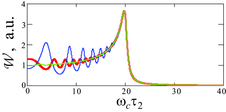
Figure S4: Energy absorbed by the flow of a highly viscous electron fluid in a long sample from an incident high-frequency field as a function of magnetic field. The calculation is made for the ac frequency $\omega\tau_{2}=40$ and the sample widths $W/l_{2}=2,4,8$ for blue, red, and green curves, respectively.

S.5 5. Non-linear response of highly viscous fluid
on dc and ac electric fields: memory effect
in relaxation at interparticle scattering

In this section we calculate the nonlinear correction to the dc flow component $V_{0}(y)$ (S36), induced by the ac component $V_{1}(y,t)$ (S40) and the memory relaxation term, $-\Gamma_{ijkl}\Pi_{kl}$, in Eqs. (S7), and the resulting mean photoconductivity $\Delta\delta\varrho_{\omega}$ of the sample.

We continue to consider the flow in a long sample with the width $W$ which is much smaller than the characteristic plasmon wavelength $l_{p}$ [see Eq. (S33)]. Similarly as for the linear component, only the $x$ component of the velocity $\mathbf{V}$ and the $xy$ components of the tensors $V_{ij}$ and $\varepsilon_{ij}$ present in the non-linear component [see Fig. 1(a) in the main text]. In such geometry, equations (S7) take the simplified form:

$$\left\{\>\begin{array}[]{l}\displaystyle\frac{\partial V}{\partial t}=\frac{e}{m}\,E^{ext}(t)-\frac{1}{m}\,\frac{\partial\Pi_{xy}}{\partial y}\\ \\ \displaystyle\frac{\partial\Pi_{xx}}{\partial t}=2\omega_{c}\Pi_{xy}-\frac{\Pi_{xx}}{\tau_{2}}-\\ \\ \displaystyle\qquad\qquad\qquad\qquad\;-\Gamma(\Delta)\,\Pi_{xx}(y,t-T)\\ \\ \displaystyle\frac{\partial\Pi_{xy}}{\partial t}=-2\omega_{c}\Pi_{xx}-\frac{\Pi_{xy}}{\tau_{2}}-\\ \\ \displaystyle\qquad\;\;-\,\,\frac{m(v^{\eta}_{F})^{2}}{4}\,\frac{\partial V}{\partial y}\,-\Gamma(\Delta)\,\Pi_{xy}(y,t-T)\end{array}\right.,$$ (S50)

where $E^{ext}(t)=E_{0}+E_{x,1}(t)$ and we used the simplest form of the retarded relaxation tensor $\Gamma_{ijkl}=\Gamma\delta_{ik}\delta_{jl}$, analogous to Eq. (S31). For the dependence of $\Gamma$ on $\Delta$, according to Eq. (S20), we write:

$$\Gamma(\Delta)=1/\tau^{\prime}_{2}-\alpha\,\Delta^{2}\>,\qquad\alpha>0\>.$$ (S51)

The positiveness of $\alpha$ corresponds to the decrease of the probability for a particle “1” to scatter again on a particle “2” with the increase of the amplitudes of the velocity $V(y,t)$, of the strain $\varepsilon_{xy}(y,t)$, and, thus, of the trajectories mismatches $\bm{\delta}_{1,2}(t)$ during a cyclotron period (see Fig. S1). Note that the same sign of the analogous parameters $\alpha$ and $\beta$ in the tensor (S3) of the memory effect in the scattering of non-interacting electrons on defects was obtained in Ref. Beltukov_Dyakonov for weak localized scatters with a smooth potential.

The mismatch $\Delta=\Delta(y,t)$ in Eqs. (S50) and (S51) is expressed via the integral of $\partial V(y,t^{\prime})/\partial y$ by Eq. (S21).

The photoconductivity and the photoresistance at small ac powers are given by the correction $I_{\omega}$ to the dc current $I_{0}$ (S38), linear by the ac power $\mathcal{W}\sim E_{1}^{2}$. Thus, together with the linear responses $I_{\omega}\sim V_{0}\sim E_{0}$ and $V_{1}\sim E_{1}$, one needs to calculate the time-independent nonlinear component $V_{\omega}(y)$ of the dc flow of the order of $\sim E_{0}E_{1}^{2}$:

$$V(y,t)=V_{0}(y)+V_{1}(y,t)+V_{\omega}(y)\>,\quad$$ (S52)

and the corresponding contribution $\hat{\Pi}_{\omega}\sim E_{0}E_{1}^{2}$ to the momentum flux tensor:

$$\hat{\Pi}(y,t)=\hat{\Pi}_{0}(y)+\hat{\Pi}_{1}(y,t)+\hat{\Pi}_{\omega}(y)\>.$$ (S53)

Here $\hat{\Pi}_{0}$ and $\hat{\Pi}_{1}$ are the linear contributions in $\hat{\Pi}$, related to $V_{0}$ and $V_{1}$ by Eq. (S28).

The equations for $\hat{\Pi}_{\omega}$ and $V_{\omega}$ are derived by the substitution of the dc and the ac linear components, $\hat{\Pi}_{0}$, $\Delta_{0}$ and $\hat{\Pi}_{1}$, $\Delta_{1}$, into the nonlinear parts of the retarded relaxation terms in Eqs. (S50) with $\Gamma(\Delta)$ (S51) and by the integration of the resulting equations for $\partial\mathbf{V}/\partial t$ and $\partial\hat{\Pi}/\partial t$ by one cyclotron period. After such procedure, we obtain:

$$\left\{\>\begin{array}[]{l}\displaystyle\frac{d\Pi_{\omega,xy}}{dy}=0\\ \\ \displaystyle\frac{\Pi_{\omega,xx}}{\tau_{2}}-2\omega_{c}\Pi_{\omega,xy}=\\ \\ \displaystyle\qquad\qquad=\alpha\,\langle\,\Delta^{2}(y,t)\,\Pi_{xx}(y,t-T)\,\rangle_{\omega}\\ \\ \displaystyle 2\omega_{c}\Pi_{\omega,xx}+\frac{\Pi_{\omega,xy}}{\tau_{2}}=-\frac{m(v^{\eta}_{F})^{2}}{4}\frac{dV_{\omega}}{dy}\,+\\ \\ \displaystyle\qquad\qquad+\,\alpha\,\langle\,\Delta^{2}(y,t)\,\Pi_{xy}(y,t-T)\,\rangle_{\omega}\end{array}\right..$$ (S54)

Here the angular brackets with the subscript “$\omega$” denote the operation of taking the contribution of the order of $\sim E_{0}E_{1}^{2}$, averaged by the last period of the ac field:

$$\langle f(t)\rangle_{\omega}=\frac{1}{T}\int_{t-T_{\omega}}^{t}dt^{\prime}\>f_{\omega}(t^{\prime})\>,$$ (S55)

where $T_{\omega}=2\pi/\omega$ is the period of the ac field and $f_{\omega}(t)=f_{12}(t)E_{0}E_{1}^{2}$ denotes the term “12” in the decomposition of the function $f(t)$ in power series by the amplitudes of the dc and the ac fields: $f(t)=\sum_{m,n=1}^{\infty}f_{mn}(t)E_{0}^{m}E_{1}^{n}$.

From the last two equations in system (S54) we obtain the expression for the nonlinear part $\hat{\Pi}_{\omega}$ of the momentum flux tensor. In particular, for its $xy$-component we have:

$$\begin{array}[]{c}\displaystyle\Pi_{\omega,xy}(y)=-m\,\eta_{xx}\frac{dV_{\omega}}{dy}+\\ \\ \displaystyle+\frac{\alpha\tau_{2}}{1+4\omega_{c}^{2}\tau_{2}^{2}}\,\big{[}\,\langle\,\Delta^{2}(y,t)\,\Pi_{xy}(y,t-T)\,\rangle_{\omega}-\\ \\ \displaystyle\qquad\quad-\,2\omega_{c}\tau_{2}\langle\,\Delta^{2}(y,t)\,\Pi_{xx}(y,t-T)\,\rangle_{\omega}\,\big{]}\>.\end{array}$$ (S56)

Here each nonlinear terms in the brackets $\langle\>..\>\rangle_{\omega}$ (S55) contain the two parts with different combinations of the dc, $V_{0}\sim\Pi_{0,ij}\sim\Delta_{0}$, and ac, $V_{1}\sim\Pi_{1,ij}\sim\Delta_{1}$, linear responses:

$$\begin{array}[]{c}\langle\,\Delta^{2}(y,t)\,\Pi_{ij}(y,t-T)\,\rangle_{\omega}=\\ \\ =\langle\,\Delta_{1}^{2}(y,t)\,\rangle\>\Pi_{0,ij}(y)\,+\\ \\ \qquad+\,\langle\,\Delta_{1}(y,t)\>\Pi_{1,ij}(y,t-T)\,\rangle\>\Delta_{0}(y)\>.\end{array}$$ (S57)

Here $ij\,=\,xx,\,xy$ and the angular brackets without a subscript denotes the operation of averaging over the last period of the ac field:

$$\langle g(t)\rangle=\frac{1}{T}\int_{t-T_{\omega}}^{t}dt^{\prime}\>g(t^{\prime})\>.$$ (S58)

The linear components of the momentum flux tensor in Eq. (S57) have the form [see Eq. (S28)]:

$$\Pi_{0,(xx/xy)}(y)=-m\,\eta_{xy/xx}\frac{dV_{0}}{dy}$$ (S59)

and

$$\Pi_{1,(xx/xy)}(y,t)=-m\,\eta_{xy/xx}\frac{dV_{1}}{dy}\,e^{-i\omega t}+c.c.\>.$$ (S60)

In view of Eq. (S49), the squared shift of the deformation $\Delta_{1}^{2}$ in Eq. (S57), averaged by $t-T_{\omega}<t^{\prime}<t$, is:

$$\langle\Delta_{1}^{2}(y,t)\rangle=\frac{4}{\omega^{2}}\sin^{2}\Big{(}\frac{\pi\omega}{\omega_{c}}\Big{)}\>\Big{|}\,\frac{dV_{1}}{dy}\Big{|}^{2}\>.$$ (S61)

Due to Eqs. (S49) and (S60), the expression under the angular brackets in the last term in Eq. (S57), averaged by $t-T_{\omega}<t^{\prime}<t$, takes the form:

$$\begin{array}[]{c}\displaystyle\langle\,\Delta_{1}(y,t)\,\,\Pi_{1,(xx/xy)}(y,t-T)\,\rangle=\\ \\ \displaystyle=\frac{2}{\omega}\>\mathrm{Re}\big{[}\,i\,\eta_{xy/xx}(\omega)\,\big{(}e^{2\pi i\omega/\omega_{c}}-1\big{)}\,\big{]}\,\Big{|}\,\frac{dV_{1}}{dy}\Big{|}^{2}\>.\end{array}$$ (S62)

Substitution of formulas (S56)-(S62) for $\Pi_{\omega,xy}$ into the first of equations (S54) leads to the final equation for the nonlinear part of the flow profile $V_{\omega}=V_{\omega}(y)$:

$$\frac{d^{2}V_{\omega}}{dy^{2}}=G(y)\>,$$ (S63)

where $G(y)$ is given by formulas (S48), (S49), and (S56)-(S62). Equation (S63) should be solved with the diffusive boundary conditions on the component $V_{\omega}(y)$: $V_{\omega}|_{y=\pm W/2}=0$. The result takes the form:

$$V_{\omega}(y)\,=\,\frac{e^{3}E_{0}E_{1}^{2}\alpha}{m^{3}(v^{\eta}_{F})^{2}}\,\frac{u+2\,\mathrm{Re}\,v}{\omega^{4}}\>J(y)\>,$$ (S64)

where $J(y)$ is the dimensionless factor determining the profile of the nonlinear flow component:

$$J(y)=\frac{|\lambda|^{2}}{|\cosh(\lambda W/2)|^{2}}\int_{|y|}^{W/2}d\tilde{y}\;\tilde{y}\;|\sinh(\lambda\tilde{y})|^{2}$$ (S65)

and the dimensionless values $u$ and $v$ contain the dependence on the frequencies $\omega$ and $\omega_{c}$:

$$u=4\sin^{2}\Big{(}\frac{\pi\omega}{\omega_{c}}\Big{)}\,(-1+4\omega_{c}^{2}\tau_{2}^{2})\>,$$ (S66)

$$\begin{array}[]{c}\displaystyle v=\frac{2\pi\omega}{\omega_{c}}\Big{[}\sin\Big{(}\frac{2\pi\omega}{\omega_{c}}\Big{)}-2i\sin^{2}\Big{(}\frac{\pi\omega}{\omega_{c}}\Big{)}\Big{]}\times\\ \\ \displaystyle\times\frac{(-1+i\omega\tau_{2}+4\omega_{c}^{2}\tau_{2}^{2})(1+4\omega_{c}^{2}\tau_{2}^{2})}{1+(4\omega_{c}^{2}-\omega^{2})\tau_{2}^{2}-2i\omega\tau_{2}}\>.\end{array}$$ (S67)

A direct calculation of the factor $J(y)$ (S65) yields:

$$\begin{array}[]{c}\displaystyle J(y)=\frac{\nu^{2}+\mu^{2}}{8\,\nu^{2}\,\mu^{2}\,\big{|}\cosh[\,(\mu-i\nu)W/2\,]\big{|}^{2}}\,\times\\ \\ \displaystyle\times\,\Big{\{}\,\mu^{2}\big{[}-\cos(\nu W)+\cos(2\nu y)\,-\\ \\ \displaystyle-\,\nu W\sin(\nu W)+2\nu y\sin(2\nu y)\,\big{]}+\\ \\ \displaystyle\quad+\,\nu^{2}\big{[}-\cosh(\mu W)+\cosh(2\mu y)\,+\\ \\ \qquad\quad+\>\mu W\sinh(\mu W)-2ty\sinh(2\mu y)\,\big{]}\,\Big{\}}\>.\end{array}$$ (S68)

where $\mu=\mathrm{Re}\,\lambda$ and $\nu=-\mathrm{Im}\,\lambda$. It is seen from Fig. S3 that both the values $\mu$ and $\nu$ are positive at any $\omega$ and $\omega_{c}$. In the limiting cases of the narrow and the wide samples, $W\ll\min(1/\mu,1/\nu)$ and $W\gg\max(1/\mu,1/\nu)$, we obtain from Eq. (S68):

$$\begin{array}[]{c}\displaystyle J(y)=\frac{(\nu^{2}+\mu^{2})^{2}}{4}\Big{[}\Big{(}\frac{W}{2}\Big{)}^{4}-y^{4}\Big{]}\end{array}$$ (S69)

and

$$\begin{array}[]{c}\displaystyle J(y)=\frac{W\,(\nu^{2}+\mu^{2})}{4\mu}\,\big{[}\,1-e^{-2\,\mu\,(\,W/2\,-\,|y|\,)}\,\big{]}\>.\end{array}$$ (S70)

In this way, in the very narrow samples the profile of the flow perturbation $V_{\omega}(y)$ is a fourth-order parabola, while in the very wide samples it is almost flat in the central region, $W/2-|y|\gg 1/\mu$, and exponentially goes to zero in the near-edge regions, $W/2-|y|\lesssim 1/\mu$. For the samples with the intermediate widths, $\min(1/\mu,1/\nu)<W<\max(1/\mu,1/\nu)$, the component $V_{\omega}(y)$ contains comparable decaying and oscillating parts [see Eq. (S68)].

The profiles $V_{\omega}(y)$ and $V_{1}(y)$ for the medium and the narrow samples are drawn in Fig. S5.

From the resulting expressions (S64)-(S68) and estimate (S23) for the coefficient in the memory term, $\alpha=B\,(R_{c}/a_{B})^{2}e^{-T/\tau_{q}}/\tau_{2}$, one can find the magnetooscillations of the velocity $V_{\omega}(y)$ at any $y$. Note that $R_{c}=v_{F}/\omega_{c}$ contains the actual Fermi velocity, unlike the viscosity coefficients containing the parameter $v_{F}^{\eta}$, $v_{F}^{\eta}\gg v_{F}$. At the strong magnetic fields and the high ac frequencies, $\omega_{c}\sim\omega\gg 1/\tau_{2}$, and far from the resonance, $|\omega-2\omega_{c}|\gg 1/\tau_{2}$, for the point $y=0$ corresponding to the typical values of $V_{\omega}(y)$ (see Fig. S3), we have:

$$V_{\omega}(0)=\sin^{2}\Big{(}\frac{\pi\omega}{\omega_{c}}\Big{)}\,V_{\omega}^{max,1}+\sin\Big{(}\frac{2\pi\omega}{\omega_{c}}\Big{)}\,V_{\omega}^{max,2}$$ (S71)

where the amplitudes of these two oscillating contributions are:

$$V_{\omega}^{max,1}=16\,\frac{e^{3}E_{0}\,E_{1}^{2}\,v_{F}^{2}}{m^{3}\,(v^{\eta}_{F})^{2}\,a_{B}^{2}}\,\frac{\tau_{2}}{\omega^{4}}\>e^{-T/\tau_{q}}\>J_{c}\>,$$ (S72)

$$\begin{array}[]{c}\displaystyle V_{\omega}^{max,2}=-\frac{4\pi\,\omega\omega_{c}}{\omega^{2}-4\omega_{c}^{2}}\>V_{\omega}^{max,1}\>,\end{array}$$ (S73)

and the dimensionless factor $J_{c}\equiv J(0)$ is:

$$J_{c}=\frac{|\lambda|^{2}}{|\cosh(\lambda W/2)|^{2}}\int\limits_{0}^{W/2}d\tilde{y}\;\tilde{y}\;|\sinh(\lambda\tilde{y})|^{2}\>.$$ (S74)

From Eq. (S68) we obtain that above the viscoelastic resonance, $\omega>2\omega_{c}$, when $\mu\ll\nu$ (see Fig. S2), the factor $J$ for different sample width is estimated as:

$$J_{c}\sim\nu^{2}W^{2}\left\{\begin{array}[]{l}\displaystyle\displaystyle\frac{1}{W\mu}\,\;,\;\;\quad W\gg 1/\mu\\ \\ \displaystyle\frac{1}{\cos^{2}(\,\nu W/2\,)}\,,\;\;1/\nu\ll W\ll 1/\mu\\ \\ \displaystyle\nu^{2}W^{2}\,,\;\;\quad W\ll 1/\nu\end{array}\right.\>.$$ (S75)

This formula for the intermediate sample widths, $1/\nu\ll W\ll 1/\mu$, is valid for the sample width far from the following condition: the coincidence of the sample width $W$ with a half-integer number of the wavelengths of transversal magnetosound vis_res_2 :

$$\nu W=\pi+2\pi l\>,$$ (S76)

where $l=0,\pm 1,\pm 2,...$. At this condition acoustic-like resonances related to standing magnetosonic modes inside the sample occur in the flow. For the sample widths, given by Eq. (S76), the denominator of $J_{c}$ in Eq. (S75) becomes zero. Therefore in the vicinities of such $\omega$ and $\omega_{c}$ one should use the exact expression for the denominator: $|\cos[\,(\nu+i\mu)\,W/2]\,|^{2}$. Thus at small values of the deviation parameter $\Delta w_{l}=\nu W/2-(\pi/2+\pi l)$, $|\Delta w_{l}|\ll 1$, and provided $\mu W\ll 1$ we have:

$$J_{c}\sim\frac{\nu^{2}W^{2}}{\Delta w_{l}^{2}+(\mu W/2)^{2}}\>.$$ (S77)

It follows from this formula that the resonances at the peculiar values of $\nu W$ (S76) can be more or less sharp depending on parameters $\omega\tau_{2}$ and $W/L_{s}$.

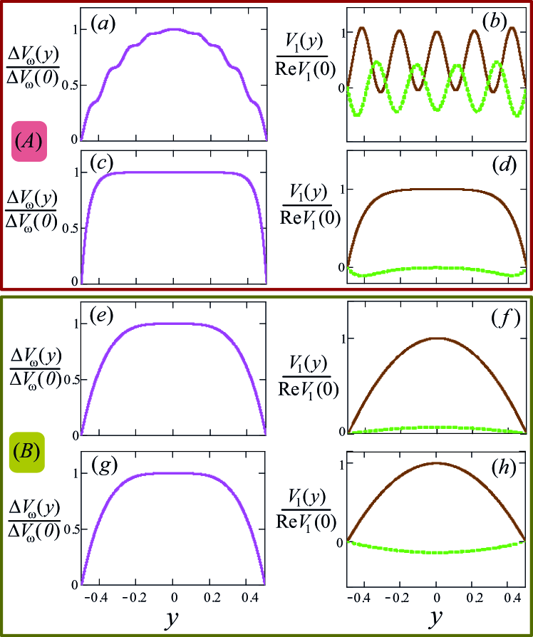
Figure S5: Profiles of the flow components $V_{\omega}(y)$ [left panels] and $V_{1}(y)$ [right panels; brown and green lines refer to $\mathrm{Re}\,V_{1}(y)$ and $\mathrm{Im}\,V_{1}(y)$, respectively]. All curves are plotted for the ac frequency $\omega\tau_{2}=40$. Panel ($A$) shows the results for a relatively wide sample, $W/L_{s}=1$, in the magnetic fields $\omega_{c}\tau_{2}=0.34$ ($a$,$b$) and $\omega_{c}\tau_{2}=0.52$ ($c$,$d$). At $\omega_{c}\tau_{2}=0.34$ the system is above the viscoelastic resonance and the wavelength and the decay length of the magnetosonic waves are: $2\pi/(L_{s}\mathrm{Im}\lambda)=0.21$ and $1/(L_{s}\mathrm{Re}\lambda)=1.004$, whereas at $\omega_{c}\tau_{2}=0.52$ the system turns out below the viscoelastic resonance that correspond to the decay length $1/(L_{s}\mathrm{Re}\lambda)=0.031$. Panel ($B$) presents the results for a narrow sample, $W/L_{s}=0.01$, at the magnetic fields $\omega_{c}\tau_{2}=0.34$ [($e$,$f$); above the resonance; $\mathrm{Im}\lambda$ and $\mathrm{Re}\lambda$ are the same as in panels ($a$,$b$)] and to $\omega_{c}\tau_{2}=0.6$ [($g$,$h$); below the resonance; $1/(L_{s}\mathrm{Re}\lambda)=0.038$].

Below the viscoelastic resonance, $\omega<2\omega_{c}$, when $\mu\gg\nu$ (see Fig. S3), one obtains from Eq. (S68):

$$J_{c}\sim\mu W\left\{\begin{array}[]{l}\displaystyle 1\,\;,\;\quad W\gg 1/\mu\\ \\ \displaystyle\mu^{3}W^{3}\,,\;\quad W\ll 1/\mu\end{array}\>.\right.$$ (S78)

From Eqs. (S42), (S43), (S74)-(S78) we estimated the amplitudes $V^{max,1/2}_{\omega}$ (S72), (S73) in an exact form for different regimes: above the viscoelastic resonance ($\omega>2\omega_{c}$) for the wide [$W\gg 1/\mu(\omega_{c})$], the medium [$1/\nu(\omega_{c})\ll W\ll 1/\mu(\omega_{c})$], and the narrow [$W\ll 1/\nu(\omega_{c})$] samples as well as below the viscoelastic resonance ($\omega<2\omega_{c}$) for the wide [$W\gg 1/\mu(\omega_{c})$] and the narrow [$W\ll 1/\mu(\omega_{c})$] samples.

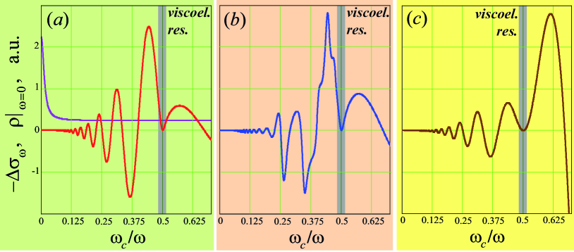
Figure S6: Photoconductivity with the inverse sign, $-\Delta\sigma_{\omega}$, for Poiseuille flows of an electron fluid with the parameters in long defectless samples. The parameters of the system are $\omega\tau_{2}=40$; $\tau_{q}/\tau_{2}=0.7$; $W/L_{s}=6,\,1.19,\,0.03$ [red, blue, and brown curves in panels ($a$-$c$), respectively]. Grey stripes schematically denote the region near the viscoelastic resonance, $\omega=2\omega_{c}$, where the fluid dynamics is mainly dissipative (in the zero approximation by $\omega\tau_{2}\gg 1$) and, thus, the elastic contribution in photoconductivity related with the perturbations of the Landau parameters $\delta F_{2,ij}$ becomes very sub (see Eq. (S7) and next Section 6). In panel ($a$) we also plotted the dc magnetoresistance $\varrho|_{\omega=0}(\omega_{c})$ (violet curve) for a sample with the same parameters of the electron fluid and some density of defects. Such magnetoresistance consists of the two contributions je_visc : the hydrodynamic one, proportional to $\eta_{xx}\sim(1+4\omega_{c}^{2}\tau_{2}^{2})^{-1}$ and dominating at $\omega_{c}\tau_{2}\lesssim 1$ ($\omega_{c}/\omega\lesssim 0.1$), and the Ohmic one, proportional to the rate of the scattering of quasiparticles on impurities, $1/\tau_{imp}$, and dominating at $\omega_{c}\tau_{2}\gg 1$ ($\omega_{c}/\omega\gg 0.1$).

We do not present all the resulting formulas for $V^{max,1/2}_{\omega}$ for these cases because of their cumbersomeness. Let us discuss in detail only the result for the most interesting regime: above the viscoelastic resonance, $\omega>2\omega_{c}\gg 1/\tau_{2}$, and for the medium sample width, $1/\nu\ll W\ll 1/\mu$, when the magnetooscillations acquire irregular shape [see Fig. 2(b) in the main text]. In this case and far from the magnetosonic resonances (S76), the velocity amplitudes (S72) and (S73) in this regimes take the form:

$$V_{\omega}^{max,1}=(\,\omega^{2}-4\omega_{c}^{2})\,V^{0}_{\omega}\,,$$ (S79)

$$V_{\omega}^{max,2}=-4\pi\,\omega\omega_{c}\,V_{\omega}^{0}\>,$$ (S80)

where

$$V_{\omega}^{0}=\frac{e^{3}E_{0}\,E_{1}^{2}\,v_{F}^{2}}{m^{3}\,(v_{F}^{\eta})^{4}\,a_{B}^{2}}\>S(\nu)\>\frac{W^{2}\,\tau_{2}}{\omega^{4}}e^{-T/\tau_{q}}$$ (S81)

and $S(\nu)\sim 1/\cos^{2}(\nu W/2)$.

Now we can find the dependencies of the radiation-induced correction $\Delta\sigma_{\omega}$ to the dc conductivity, $\sigma=\sigma_{0}+\Delta\sigma_{\omega}$, on temperature, ac frequency, and magnetic field far from the magnetosonic resonances (S76). The value $\Delta\sigma_{\omega}$ is defined as:

$$\Delta\sigma_{\omega}=\frac{I_{\omega}}{E_{0}W}\>,\qquad I_{\omega}=en_{0}\int_{-W/2}^{W/2}dy\>V_{\omega}(y)\>.$$ (S82)

Equations (S74)-(S71) and (S79)-(S81) yield for the photoconductivity $\Delta\sigma_{\omega}$ in the considered case, $1/\nu\ll W\ll 1/\mu$, when the standing magnetosonic waves are well-formed:

$$\Delta\sigma_{\omega}=(U+V)\,\Delta\sigma_{\omega}^{max}\>,$$ (S83)

where the factors $U=U(\omega/\omega_{c})$ and $V=V(\omega/\omega_{c})$ are:

$$\begin{array}[]{c}\displaystyle U=\Big{[}1-\Big{(}\frac{2\omega_{c}}{\omega}\Big{)}^{2}\Big{]}\,\sin^{2}\Big{(}\,\frac{\pi\omega}{\omega_{c}}\,\Big{)}\>,\\ \\ \displaystyle V=-\frac{4\,\pi\,\omega_{c}}{\omega}\,\sin\Big{(}\,\frac{2\pi\omega}{\omega_{c}}\,\Big{)}\>,\end{array}$$ (S84)

and the amplitude $\Delta\sigma_{\omega}^{max}=\Delta\sigma_{\omega}^{max}(\,\omega,\,\omega_{c}\tau_{q}\,)$ is:

$$\Delta\sigma_{\omega}^{max}\sim\frac{e^{4}E_{1}^{2}\,n_{0}\,v_{F}^{2}}{m^{3}\,(v_{F}^{\eta})^{4}\,a_{B}^{2}}\,\frac{W^{2}\tau_{2}}{\omega^{2}}\>{\Large e}^{-2\pi/(\omega_{c}\tau_{q})}\>.$$ (S85)

Here the relaxation times $\tau_{q}=\tau_{q}(T_{e})$ and $\tau_{2}=\tau_{2}(T_{e})$ are given by Eqs. (S24). It follows from this result that the oscillation of photoconductivity are suppressed with the increase of the temperature $T_{e}$ and the ac frequency $\omega$.

One can see from Eq. (S77) that in the vicinities of the magnetosonic resonances (S76) the value $\Delta\sigma_{\omega}^{max}\sim J_{c}$ increases as compared with Ref. (S85) in the large factor $\nu^{2}/\mu^{2}\gg 1$.

In Fig. S6 we present the averaged photoconductivity $\Delta\sigma_{\omega}$ (S82) multiplied on $-1$ (this value is presented as photoresistance in linear by the ac power $\mathcal{W}$ approximation is $\Delta\delta\varrho_{\omega}=-\Delta\sigma_{\omega}/\sigma_{0}^{2}$). The curves are plotted at a fixed ac frequency $\omega$ and the sample widths $W$ smaller, comparable, and larger than the characteristic decay length $L_{s}$. The dependence $-\Delta\sigma_{\omega}(\omega_{c})$ exhibits oscillations by the inverse magnetic field. The shape of the obtained oscillations is sinusoidal in the limiting cases $W\gg L_{s}$ and $W\ll L_{s}$, while for intermediate sample widths, $W\sim L_{s}$, it is irregular. The last property is related to the appearance of the magnetosonic resonances in the ac linear response $V_{1}(y,t)$ at the sample width satisfying conditions (S76). These resonances manifest themselves most clearly when $W\sim L_{s}$ and, thus a not too many wavelengths fit in the sample, but the damping of waves is relatively weak.

S.6 6. Non-linear response of highly viscous fluid
on dc and ac electric fields: memory effect
in elastic part of interparticle interaction

In this section, we calculate the “elastic” contribution in the nonlinear correction $V_{\omega}$ to the dc velocity $V_{0}(y)$, which originates from the retarded nonlinear by $\mathbf{V}(\mathbf{r},t)$ part of the energy of quasiparticles. This contribution is additive to the “inelastic” contribution in $V_{\omega}$ from retarded relaxation due to the memory effect in extended collisions, calculated in the previous section. The elastic contribution in $V_{\omega}$ calculated below also leads to photoresistance, whose properties however are partially different from the ones of inelastic contribution.

The equations for $\hat{\Pi}_{\omega}$ and $V_{\omega}$ are derived by the substitution of the dc and the ac linear components, $\hat{\Pi}_{0}$, $\Delta_{0}$ and $\hat{\Pi}_{1}$, $\Delta_{1}$, into the nonlinear parts of the retarded elastic terms in Eqs. (S7) with $\delta F_{2,ij}$ (S51). Herewith, for simplicity, we consider that $F_{2}=0$ in the left part of Eq. (S7). For the flat geometry of Poiseuille flow, the resulting equation become similar to Eqs. (S50) accounting the retarded relaxation via the terms $\sim\hat{\Gamma}$. Then one should integrate the resulting equations for $\partial\mathbf{V}/\partial t$ and $\partial\hat{\Pi}/\partial t$ by one cyclotron period, as it was done in the previous section. After such procedure, we obtain:

$$\left\{\>\begin{array}[]{l}\displaystyle\frac{1}{m}\frac{d\Pi_{\omega,xy}}{dy}=0\\ \\ \displaystyle\frac{\Pi_{\omega,xx}}{\tau_{2}}-2\omega_{c}\Pi_{\omega,xy}\,=\\ \\ \displaystyle\qquad\quad\quad\quad=\,\Big{\langle}F_{2,xx}^{(1)}(y,t)\,\frac{\partial\Pi_{xx}(y,t)}{\partial t}\,\Big{\rangle}_{\omega}\\ \\ \displaystyle 2\omega_{c}\Pi_{\omega,xx}+\frac{\Pi_{\omega,xy}}{\tau_{2}}=-\,\frac{m_{0}\,(v^{\eta}_{F})^{2}}{4}\frac{dV_{\omega}}{dy}\,+\\ \\ \displaystyle\qquad\quad\quad\quad\;+\,\Big{\langle}\delta F_{2,xy}^{(1)}(y,t)\,\,\frac{\partial\Pi_{xy}(y,t)}{\partial t}\,\Big{\rangle}_{\omega}\end{array}\right..$$ (S86)

In these formulas all notations are the same as in the previous section.

From the last two equations in system (S86) we obtain the expression for the nonlinear part $\hat{\Pi}_{\omega}$ of the momentum flux tensor. For the $xy$-component we have:

$$\begin{array}[]{c}\displaystyle\Pi_{\omega,xy}(y)=-m_{0}\,\eta_{xx}\frac{dV_{\omega}(y)}{dy}\,+\\ \\ \displaystyle+\,\frac{\tau_{2}}{1+4\omega_{c}^{2}\tau_{2}^{2}}\,\big{[}\,\Big{\langle}\delta F_{2,xy}^{(1)}(y,t)\,\,\frac{\partial\Pi_{xy}(y,t)}{\partial t}\,\Big{\rangle}_{\omega}-\\ \\ \displaystyle\qquad\quad-\,2\omega_{c}\tau_{2}\Big{\langle}\delta F_{2,xx}^{(1)}(y,t)\,\,\frac{\partial\Pi_{xx}(y,t)}{\partial t}\,\Big{\rangle}_{\omega}\,\big{]}\>.\end{array}$$ (S87)

Here the nonlinear terms in the brackets $\langle\>..\>\rangle_{\omega}$ (S55) again contain the two contributions with the different combinations of the dc and ac linear responses:

$$\begin{array}[]{c}\displaystyle\Big{\langle}\delta F_{2,xx}^{(1)}(y,t)\,\,\frac{\partial\Pi_{xx}(y,t)}{\partial t}\,\Big{\rangle}_{\omega}=\\ \\ \displaystyle=\Big{[}\,a\,\Big{\langle}\,\Pi_{1,xx}(y,t-T)\,\frac{\partial\Pi_{1,xx}(y,t)}{\partial t}\,\Big{\rangle}\,+\\ \\ \displaystyle+\,b\,\Big{\langle}\,\Pi_{1,xy}(y,t-T)\,\frac{\partial\Pi_{1,xx}(y,t)}{\partial t}\,\Big{\rangle}\,\Big{]}\,\frac{dV_{0}(y)}{dy}\>,\end{array}$$ (S88)

and

$$\begin{array}[]{c}\displaystyle\Big{\langle}\delta F_{2,xy}^{(1)}(y,t)\,\,\frac{\partial\Pi_{xx}(y,t)}{\partial t}\,\Big{\rangle}_{\omega}=\\ \\ \displaystyle=\Big{[}\,c\,\Big{\langle}\,\Pi_{1,xx}(y,t-T)\,\frac{\partial\Pi_{1,xy}(y,t)}{\partial t}\,\Big{\rangle}\,+\\ \\ \displaystyle+\,d\,\Big{\langle}\,\Pi_{1,xy}(y,t-T)\,\frac{\partial\Pi_{1,xy}(y,t)}{\partial t}\,\Big{\rangle}\,\Big{]}\,\frac{dV_{0}(y)}{dy}\>,\end{array}$$ (S89)

At the considered regime of high frequencies and magnetic fields, $\omega\sim\omega_{c}\gg 1/\tau_{2}$, the viscosity coefficients are related as $-i\omega\eta_{xy}(\omega)\approx 2\omega_{2}\eta_{xx}(\omega)$. After substitution if the expression for $\hat{\Pi}_{1}$ via $\mathbf{V}_{1}$ and averaging over the interval $t-T<t^{\prime}<t$, the values in Eqs. (S88) and (S89) takes the form:

$$\Big{\langle}\,\Pi_{1,ij}(y,t-T)\,\frac{\partial\Pi_{1,kl}(y,t)}{\partial t}\,\Big{\rangle}=Q_{ij,kl}\,R(y)$$ (S90)

where

$$\begin{array}[]{c}\displaystyle Q_{xx,xx}\\ \\ Q_{xy,xy}\end{array}\Bigg{\}}\,=\,-\frac{2}{\omega}\,\sin\Big{(}\frac{2\pi\omega}{\omega_{c}}\Big{)}\Bigg{\{}\begin{array}[]{c}\displaystyle 4\,\omega_{c}^{2}\\ \\ \omega^{2}\end{array}\>,$$ (S91)

$$\begin{array}[]{c}\displaystyle Q_{xx,xy}=Q_{xy,xx}=4\,\omega_{c}\,\cos\Big{(}\frac{2\pi\omega}{\omega_{c}}\Big{)}\>,\end{array}$$ (S92)

and

$$R(y)=|\eta_{xx}(\omega)|^{2}\>\Big{|}\,\frac{dV_{1}(y)}{dy}\Big{|}^{2}$$ (S93)

Substitution of formulas (S87)-(S93) for $\Pi_{\omega,xy}$ into the first of equations (S86) leads to the final equation for the nonlinear component $V_{\omega}=V_{\omega}(y)$ of the dc velocity:

$$\frac{d^{2}V_{\omega}}{dy^{2}}=H(y)\>,$$ (S94)

where $H(y)$ is given by Eqs. (S87)-(S92). Equation (S94) should be solved with the diffusive boundary conditions on the component $V_{\omega}(y)$: $V_{\omega}|_{y=\pm W/2}=0$. The result takes the form:

$$V_{\omega}(y)=\frac{e^{3}E_{0}E_{1}^{2}}{m_{0}^{3}(v^{\eta}_{F})^{2}}\>\frac{|\eta_{xx}(\omega)|^{2}}{\omega\,\eta_{xx}}\>\Phi(\omega,\omega_{c})\,J(y)\>,$$ (S95)

where the factor $J(y)=J(y,\lambda)$, determining the shape of $V_{\omega}(y)$, is the same [Eq. (S65)], as for the inelastic contribution and the factor $\Phi(\omega,\omega_{c})$ has the form:

$$\begin{array}[]{c}\displaystyle\Phi=4\>\Big{\{}\,\Big{[}-a\,\omega_{c}\tau_{2}+2d\,\Big{(}\frac{\omega_{c}}{\omega}\Big{)}^{2}\Big{]}\,\sin\Big{(}\frac{2\pi\omega}{\omega_{c}}\Big{)}+\\ \\ \displaystyle+\,\Big{[}-2b\,\omega_{c}\tau_{2}+c\,\Big{]}\,\frac{\omega_{c}}{\omega}\,\cos\Big{(}\frac{2\pi\omega}{\omega_{c}}\Big{)}\,\Big{\}}\>.\end{array}$$ (S96)

We remind that the coefficients $a,b,c,d$ are proportional to the probability $P$ (S11) for two quasiparticles in a pair to make a complete cyclotron rotation without scattering on a third quasiparticle.

The resulting dependence of the elastic contribution to the sample photoconductivty on magnetic field at fixed $\omega$ exhibits MIRO-like oscillations at $\omega_{c}<\omega/2$ and a huge peak near $\omega_{c}=\omega/2$ (see Fig. 3 in the main text). By the last feature, it differs from the inelastic contribution, which has no peak at $\omega_{c}=\omega/2$.

S.7 7. Discussion of model and results

7.1. Independence of photoresistance on the sign of circular polarization of radiation

As it was discussed in the main text, the dependencies of $\Delta\sigma_{\omega}$ and $\Delta\varrho_{\omega}$ on the polarization sign are absent for the case of purely hydrodynamic flows in the defectless and narrow samples, $W\ll l_{p}$ (S33). In this case, the viscoelastic contribution dominates in the ac flow, the component $E_{1,y}^{ext}$ of the external electric field is screened inside the sample, and the velocity $\mathbf{V}_{1}\,||\,\mathbf{e}_{x}$ becomes independent of $E_{1,y}^{ext}$ and the helicity of polarization.

For Ohmic flows in wide bulk samples the situation is totally different. In theory Beltukov_Dyakonov and other theories for disordered samples it is implied that the ac electric field acting on independent electrons in Ohmic samples is just the external radiation field $\mathbf{E}_{1}(t)$. Unlike the current hydrodynamic model, the memory term due to extended collisions of electrons with localized defects in the equation for $\partial\mathbf{V}/\partial t$ contains not the mismatch of the deformation, $\hat{\Delta}(\mathbf{r},t)$, but the mismatch of the electron position, $\mathbf{r}_{0}(t)$, after one cyclotron rotation, $\bm{\Delta}(t)=\mathbf{r}_{0}(t)-\mathbf{r}_{0}(t-T)$. Such mismatch $\bm{\Delta}\neq 0$ arises due to the force $e\mathbf{E}_{0}+e\mathbf{E}_{1}(t)$ from external electric fields, directly acting on electrons between their collisions with defects. Obviously, $\bm{\Delta}(t)$ and the resulting photoconductivity strongly depend on the sign $\pm$ of the polarization of $\mathbf{E}_{1}(t)$ Beltukov_Dyakonov ; rev_M .

Thus, the independence of the photoresistance of the sign $\pm$ of circular polarization is a necessary (but not sufficient) evidence of the formation of a high-frequency hydrodynamic flow of a viscous electron fluid. The dependence on $\pm$ can appear in sufficiently wide samples, $W\gtrsim l_{p}$, owing to the formation of a substantial plasmonic component in $V_{1}$, or at a sufficiently large strength of disorder when the main contribution to photoconductivity becomes related to the scattering of single quasiparticles on defects or the sample edges.

In Ref. rev_M the following idea about the explanation of the absence of the dependence of MIRO on the helicity of the circular polarization of an incident radiation field $\mathbf{E}_{1}^{ext}(t)$ was formulated. The difference of the polarization of the actual ac field $\mathbf{E}_{1}(\mathbf{r},t)=\mathbf{E}_{1}^{ext}(t)+\mathbf{E}_{1}^{int}(\mathbf{r},t)$, which is “felt” by 2D electrons, and the polarization of the incident field $\mathbf{E}_{1}^{ext}(t)$ can be induced by some elements of an experimental setup. This can result in an independence (more exactly, a weak dependence) of MIRO on the sign of the polarization of $\mathbf{E}_{1}^{ext}(t)$. However, it was not indicated in Ref. rev_M that this modification of the polarization can be a consequence of the screening of one of the components of the incident field $\mathbf{E}_{1}^{ext}(t)$ by the internal ac field $\mathbf{E}_{1}^{int}(\mathbf{r},t)$ originating from the redistribution of the very 2D electron fluid density $\delta n(\mathbf{r},t)$ and, thus, can be inextricably related with the mechanism of MIRO. It is noteworthy that in Ref. Savchenko it was experimentally demonstrated that particular setups of experiments (shapes of samples, designs of ac radiation sources) indeed can sufficiently change the sensitivity of the MIRO effect relative to the polarization of the external radiation $\mathbf{E}_{1}^{ext}(t)$. However, in experiment Savchenko an almost complete independence of photoresistance on the helicity of the circularly polarized radiation, which was observed, for example, in Ref. Smet_1 , was not achieved I_A_Dmitriev_private_communication .

In Refs. Mikhailov ; Chepelianskii_Shepelyansky theories of another type for 2D electron magnetotransport were developed, in which the photoresistance is associated with the ac-field-induced redistribution of the electron density near sample contacts Mikhailov or around localized defects inside a sample Chepelianskii_Shepelyansky . Although these theories lead to magnetooscillations of photoresistance with a weak dependence on the sign of the circular polarization of the incident radiation, there exist substantial problems in the comparison of other predictions of those theories with experiments on MIRO. For example, there is a discrepancy between the shapes of the predicted oscillations and of the oscillations observed in experiments. The latter ones are often sinusoidal, whereas in Refs. Mikhailov ; Chepelianskii_Shepelyansky the sinusoidal shape of magnetooscillations was not obtained.

7.2. Mixed hydrodynamic-Ohmic flows

Below we study how the particular violation of the “maximal” conditions of the applicability of the developed purely hydrodynamic model, the absence of bulk disorder and a very large strength of the interparticle interaction, can be relaxed so that the obtained above key results on photoresistance of a highly viscous fluid remain qualitative valid.

In this subsection, we estimate the parameters of a long disordered sample at which the hydrodynamic contributions to the ac and nonlinear flow components persist, despite of the dominance of the Ohmic contribution in the dc flow component.

At high magnetic fields, $\omega_{c}\tau_{2}\gg 1$, the magnitude of a purely hydrodynamic dc flow unlimitedly increases, being proportional to $\omega_{c}^{2}$ [Eqs. (S36) and (S37)]. Thus the purely hydrodynamic dc averaged resistance: $\varrho_{0}=E_{0}W/I_{0}$ strongly decreases with the increase of $\omega_{c}$ and $W$:

$$\varrho_{0}\,\propto\,1\,/\,(W\omega_{c})^{2}\>.$$ (S97)

Such divergence is limited by the formation of an Ohmic flow in central region of the sample where the scattering of quasiparticles on disorder (and/or phonons) becomes to dominate and to determine the magnitude of the current and the resistance $\varrho_{0}$ {see Refs. je_visc ; Alekseev_Dmitriev and Fig. S6(a)}.

The Ohmic contribution in the dc current $I_{0}$ dominates if the sample width is much larger than the Gurzhi length $l_{G}=l_{G}(\omega_{c})$:

$$W\gg l_{G}\>,\quad l_{G}=\sqrt{\tau_{tr}\eta_{xx}(\omega_{c})}\>,$$ (S98)

where $\tau_{tr}$ is the total momentum relaxation time due to the scattering of quasiparticles on bulk disorder and acoustic phonons. In this case, the Ohmic part of the flow is located in the central sample region:

$$-W/2+l_{G}\lesssim y\lesssim W/2-l_{G}\>,$$ (S99)

or, more precisely, $W/2-|y|\gg l_{G}$. The resulting hydrodynamic-Ohmic magnetoresistance has the form {see Fig. S6(a) and discussion in Ref. je_visc }:

$$\varrho_{0}(B)\sim\frac{\eta_{xx}(B)}{W^{2}}+\frac{1}{\tau_{tr}}\>.$$ (S100)

One can show that at the considered high-frequency regime, $\omega_{c}\sim\omega\gg 1/\tau_{2}$, the inequality (S98) is consistent with inequality (S33), which ensures the dominance of the viscoelastic pact in the ac component, provided the condition:

$$s\,\gg\,v_{F}^{\eta}\sqrt{\frac{\tau_{tr}}{\tau_{2}}}\>.$$ (S101)

Here $s$ is the velocity if plasmons for the structures with 2D electrons near a metallic gated. Although for applicability of the presented above hydrodynamic description of the viscoelastic component one needs $v_{F}^{\eta}\gg v_{F}$, these two parameters, apparently, do not differ too much at realistic electron densities $n_{0}\sim 10^{11}-10^{12}$ cm^-2 in GaAs quantum wells recentest_ ; Alekseev_Dmitriev . Herewith the plasmon velocity $s\sim n_{0}^{1/2}$ is usually far greater than $v_{F}$ Semiconductors . Thus condition (S101) can be typically fulfilled in such GaAs structures. It follows from the above conditions that for the frequencies $\omega\sim\omega_{c}$ in the interval:

$$\frac{v_{F}^{\eta}\sqrt{\tau_{tr}}}{W\sqrt{\tau_{2}}}\ll\omega\ll\frac{s}{W}\>,$$ (S102)

the dc current component $I_{0}$ is predominantly due to the Ohmic flow $V_{0}(y)\approx const$ in the central (bulk) region (S99), whereas the ac flow component is still formed mainly by the magnetosonic waves in the whole sample.

For such flows, only in the near-edge regions:

$$y\,:\;\;W/2-|y|\lesssim l_{G}\>,$$ (S103)

both the dc and ac flow components $V_{0}(y)$ and $V_{1}(y,t)$ are controlled by viscosity and viscoelasticity. In the bulk region  (S99) the dc component of the flow ia homogeneous, $V_{0}(y)=const$, thus values (S57), (S88) and (S89), determining the elastic and the inelastic parts of $V_{\omega}(y)$, are zero, and the bulk region provides no hydrodynamic contributions to photoresistance.

Now we are able to estimate the magnitude of the hydrodynamic contribution to photoconductivity $\Delta\sigma_{\omega}$ from the near-edge regions (S103), originating only from the memory effect in the interparticle scattering (see Section 2). For a rough estimate, we can use the derived above formulas for $\Delta\sigma_{\omega}$ of a Poiseuille flow, changing in them the sample width $W$ on the characteristic width of the near-edge regions, $l_{G}$ (S98). Herewith we neglect the contribution to photoconductivity from the bulk region (S99), which is controlled by disorder. Our estimations based on Eqs. (S85) for $\Delta\sigma_{\omega}|_{W=l_{G}}$ and on the formulas from Refs. rev_M and Beltukov_Dyakonov for photoconductivity due to the memory effects in scattering on disorder show that this assumption can be realistic.

In this way, when the Ohmic contribution in the dc conductivity $\sigma_{0}$ and the hydrodynamic contribution $\Delta\sigma_{\omega}$ of the near edge-layers (S103) in the nonlinear photoconductivity dominate, the averaged photoresistivity in the linear by ac power regime, $\Delta\varrho_{\omega}\sim E_{1}^{2}$, takes the form:

$$\Delta\varrho_{\omega}=-\Delta\sigma_{\omega}/\sigma_{0}^{2}\>,$$ (S104)

where $\Delta\sigma_{\omega}$ is calculated by Eqs. (S83)-(S85) and (S95), while the averaged dc conductivity $\sigma_{0}$ of a sample is close to the Ohmic conductivity of the bulk region (S99):

$$\sigma_{0}=e^{2}n_{0}\tau_{tr}/m\>.$$ (S105)

Note that the last value has no dependence on magnetic field, the electron temperature, and the sample width.

Equation (S104) leads to an estimate for the dependence of the photoresistivity on magnetic field, ac frequency, and the electron temperature.

For example, for the inelastic relaxation contribution $\Delta\sigma_{\omega}^{rel}$ due to the extended collisions of quasiparticle pairs (see Fig. S1), in the interval of the magnetic fields corresponding to the inequality $1/\nu\ll l_{G}(\omega_{c})\ll 1/\mu$ [and, thus, to the applicability of Eq. (S85)], equations (S83)-(S85), (S98), (S104), and (S105) yield:

$$\begin{array}[]{c}\displaystyle\Delta\varrho_{\omega}^{rel}=\sin^{2}\Big{(}\frac{\pi\omega}{\omega_{c}}\Big{)}\>\Delta\varrho^{max,1}_{\omega}+\\ \\ \displaystyle+\sin\Big{(}\frac{2\pi\omega}{\omega_{c}}\Big{)}\>\Delta\varrho^{max,2}_{\omega}\>,\end{array}$$ (S106)

where

$$\Delta\varrho^{max,1}_{\omega}=-\displaystyle\frac{A_{O}}{\omega^{2}\omega^{2}_{c}}\,\Big{(}\,1-\frac{4\omega_{c}^{2}}{\omega^{2}}\Big{)}\>{\displaystyle e}^{-A_{E}T_{e}^{2}/\omega_{c}}\>,$$ (S107)

and

$$\Delta\varrho^{max,2}_{\omega}=\displaystyle\frac{4\pi A_{O}}{\omega^{3}\omega_{c}}\,\>{\displaystyle e}^{-A_{E}T_{e}^{2}/\omega_{c}}\>.$$ (S108)

Here the coefficients $A_{O}$ and $A_{E}$ are independent of $\omega$, $\omega_{c}$, $T_{e}$ and are easily calculated from Eqs. (S85), (S98), and (S105). It is seen from Eqs. (S107) and (S108) that at $1<\omega/\omega_{c}<4\pi$ the first amplitude, $\Delta\varrho^{max,1}_{\omega}$, is numerically smaller than the second one, $\Delta\varrho^{max,2}_{\omega}$.

7.3. Case of weak interparticle interaction

In this subsection, we discuss the possibility of weakening of the condition about a very large strength of the interparticle interaction, which allows the simple viscoelastic equations (S7) of a highly viscous fluid.

It is known that the shear stress transversal sound can be excited in an electron fluid in zero magnetic field not only at the very low densities $n_{0}$ corresponding to $r_{s}\gg 1$ and to large Landau parameters: $F_{m}\gg 1$, but also at moderate densities, when $r_{s}\sim 1$ and $F_{m}\sim 1$ LP ; Kho . In the latter case, a high-frequency flow of the fluid is described not only by the hydrodynamic variables $n$, $\mathbf{V}$, and $\hat{\Pi}$, but by the whole distribution function $f(\mathbf{r},t,\mathbf{v})$ of the Fermi-liquid quasiparticles. A decomposition of such $f(\mathbf{r},t,\mathbf{v})$ by the angle $\varphi$ of the quasiparticle velocity $\mathbf{v}$ contains many comparable angular harmonics $e^{im\varphi}$. (We remind that the hydrodynamic description by the variables $n$, $\mathbf{V}$, and $\hat{\Pi}$ implies the predomination of the zero, the first, and the second harmonics by $\mathbf{v}$ in $f$.) The shear-stress transverse waves in 3D and 2D Fermi liquid can be excited if the Landau parameters $F_{m}$ are greater than some critical values $F_{m,c}\sim 1$ LP ; Kho . In Refs. vis_res_2 ; Semiconductors similar transverse waves in the presence of magnetic field were studied for a strongly non-ideal electron Fermi liquid, in which $F_{m}\gg 1$. Apparently, the results of Refs. vis_res_2 ; Semiconductors are qualitatively valid also for moderate interparticle interaction, when $F_{m}\sim 1$.

Possibly, formation in magnetic field of the pairs of colliding quasiparticles (see Figs. S1,S2) may additionally enhance the degree of internal coherence in the electron fluid, that is reflected in the increases of correlations in the quasiparticle dynamics and of the role of the viscoelastic effects. We hypothesize that such system may be described within some effective Fermi-liquid-like model with renormalized Landau parameter $\widetilde{F}_{1}$ and $\widetilde{F}_{2}$, which are large: $\widetilde{F}_{1,2}\gg 1$. As a consequence, the transversal magnetosonic waves may survive even when the “ordinary” one-quasiparticle Landau parameters are small: $F_{1,2}\ll 1$. In such case the excitation of magnetosonic waves may lead to the peculiar photoconductivity, similar to the one of an “ordinary” highly viscous fluid, in which $F_{1,2}\gg 1$ [the case studied in Sections 1-6].

Consideration of the last effects may be an important subject for future microscopic theories of the highly viscous electron fluid.

S.8 8. Additional comparison with experiments

8.1. Simultaneous observation of peak at doubled cyclotron frequency and giant negative magnetoresistance

First of all, we note that the strong giant negative magnetoresistance and the irregular shape of MIRO, including the peak near $\omega=2\omega_{c}$, are usually observed in the same highest mobility samples up to the lowest temperatures (see experiments Smet_1 ; Ganichev_1 ; exp_GaAs_ac_1 ; exp_GaAs_ac_2 and, especially, recent experiment recentest_ ). This fact, apparently, point out on the realization of the hydrodynamic transport regime in both the dc and ac components of a flow in 2D electron systems in the same samples. In particular, the formation of the highly viscous fluid, in which the transversal magnetosound can be exited, also manifests itself by the giant negative magnetoresistance, which was initially predicted for the flows of an ordinary viscous electron fluid je_visc ; Gurzhi_Shevchenko . This statement is illustrated in the main text by the experimental data on magnetoresistance and photoresistance [Figs. 3(B,C)] and in Fig. S6(a) by the theoretical dependence $\varrho_{0}(B)$ corresponding to Eq. (S100).

8.2. Dependencies of oscillating part of photoconductivity and photoresistance on electron temperature

The temperature and magnetic field dependencies of the amplitude of MIRO observed in Ref. Zudov_T for a high-mobility GaAs quantum very well correspond to Eq. (S108), including the absence of a temperature dependence in the pre-exponent factor $A_{O}$. The formula used in Ref. Zudov_T for fitting of the MIRO amplitude was just the same as Eq. (S108).

Herewith we note that, a substantial temperature dependence of the pre-exponent amplitude of phonotoresistance oscillations was reported in experimental works S5 ; W . This result may not contradict to the correspondence of theoretical result (S106)-(S108) to experiment Zudov_T by the following reasons. First, experiment W was performed for the GaAs structures with double quantum wells, where all the discussed effects may be quite different. Second, in Ref. S5 rather different formulas for fitting of MIRO were used, as compared with Eq. (S106) and the formulas used in Ref. Zudov_T , so the results of Ref. S5 cannot be directly compared with the results of Ref. Zudov_T and the predictions of our theory.

In this way, the results on the temperature dependence of MIRO experimentally obtained in Ref. Zudov_T can be explained by the model of a mixed Ohmic-hydrodynamic flow, developed in Section 7.2 and leading to photoresistance (S106)-(S108).

8.3. Behavior of MIRO with varying of ac frequency

With the increase of the frequency $\omega$, the shape of the oscillations of $\Delta\varrho_{\omega}$ as the function of the ratio $\omega/\omega_{c}$ is retained in our theory [see Eqs. (S106)-(S108)]. The pre-exponent factor in the larger contribution $\Delta\varrho^{max,2}_{\omega}$ (S108) at a fixed ratio $\omega/\omega_{c}$ is rapidly suppressed with $\omega$ as $\sim 1/\omega^{4}$:

$$\frac{\Delta\varrho^{max,2}_{\omega}}{(\omega/\omega_{c})\>e^{-B\,T_{e}^{2}/\omega_{c}}}=\displaystyle\frac{4\pi A_{O}}{\omega^{4}}\,\>.$$ (S109)

Beside this, the destructive “geometric” effects from inhomogeneities of the sample edges and from possible macroscopic defects inside the sample on the formation of the standing waves in the ac flow component become more and more substantial with the increase of $\omega$. Indeed, the characteristic wavelength, $l_{s}=v_{F}^{\eta}/\omega$, which should be grated than the sample inhomogeneities in order to form the standing magnetosonic waves, decreases with $\omega$. So a suppression and a smearing of the ac flow component and of its contribution to magnetooscillations of $\Delta\varrho_{\omega}$ are expected with the increase of $\omega$.

These predictions are in a good agreement with the measurements of MIRO in a high-mobility GaAs quantum well at the different frequencies $\omega$ in Ref. S5 .

8.4. Comparison of departure time $\tau_{q}$ with the shear stress relaxation time $\tau_{2}$

The departure times $\tau_{q}$ (S2) and (S11) controls the amplitude of MIRO via the probability $P=e^{-T/\tau_{q}}$. It is of interest to compare the experimental value of $\tau_{q}$ with the experimental value of the shear stress relaxation time $\tau_{2}$, which determine the magnitude and the magnetic field dependence of the viscosity coefficients $\eta_{xx,xy}|_{\omega=0}$.

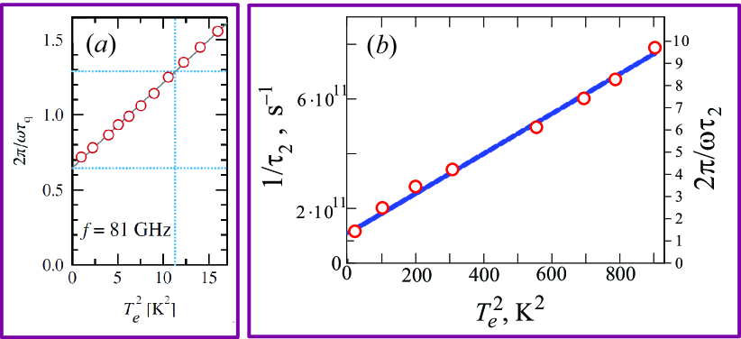
Figure S7: (a) Experimental data on the departure scattering time $\tau_{q}$ as a function of temperature $T_{e}$, obtained from the measurements of the amplitude of MIRO in a high-mobility GaAs quantum well with the 2D electron density $n_{0}=2.8\cdot 10^{11}$ cm^-2 ($r_{s}=1.05$). Thin solid line is the quadratic fit $a_{q}+b_{q}T_{e}^{2}$. The picture is taken from Ref. Zudov_T . (b) Shear stress relaxation time $\tau_{2}$ at different $T_{e}$ obtained from fitting of the giant negative magnetoresistance measured in Ref. exps_neg_4 in a high-mobility GaAs/AlGaAs quantum well with the same $n_{0}$. Blue solid line is the quadratic fit $a_{2}+b_{2}T_{e}^{2}$. Right vertical scale shows the values $1/\tau_{2}$ in the same units as in panel ($a$) [i. e., divided by the ac frequency from panel ($a$)].

In Fig. S7 we present experiential data for the GaAs quantum wells in the two different samples with the close electron densities $n_{0}$ corresponding to the intermediate interaction parameter $r_{s}\approx 1.05$. In panel ($a$) we cite the data on the departure scattering time $\tau_{q}(T_{e})$ obtained in Ref. Zudov_T from the measurements of the temperature dependence of the MIRO amplitude $\Delta\varrho_{\omega}$. This value was supposed to be proportional to $P=e^{-T/\tau_{q}}$ with the departure time being quadratic by temperature: $\tau_{q}(T_{e})\sim 1/T_{e}^{2}$. In panel ($b$) we plot experimental data on the shear stress relaxation time $\tau_{2}(T_{e})$ extracted by us from the giant negative magnetoresistance of 2D electron fluid measured in Ref. exps_neg_4 in a GaAs quantume well. To obtain the experimental values of $\tau_{2}$, we used the fitting of the negative magnetoresistance by the procedure proposed in Refs. Alekseev_Dmitriev ; je_visc . Both the rates $1/\tau_{q}(T_{e})$ and $1/\tau_{2}(T_{e})$ are indeed approximately quadratic by the electron temperature $T_{e}$ and have some residual values in the limit $T_{e}\to 0$. The temperature-dependent part of $\tau_{q}$ is in several times shorter than the one of $\tau_{2}$. This is consistent with the calculations of these times within the kinetic equation exactly accounting the interparticle scattering Novikov ; Alekseev_Dmitriev .

Comparable experimental values of $\tau_{q}$ and $\tau_{2}$ as well as the inequality $\tau_{q}<\tau_{2}$ evidence in favor of the hydrodynamic nature of the magnetoresistance and magnetoscillations of the photoresistance in the samples studied in Refs. Zudov_T ; exps_neg_4 . However, as it was mentioned in Section 7.3, for a quantitative description of the experimental data for samples with the interaction parameter $r_{s}\lesssim 1$, a more rigorous accounting of the correlations due to formation of the quasiparticle pairs is needed.

8.5. Role of disorder in narrow samples

Let us discuss the role of “residual disorder” in the relatively narrow samples, $W\ll l_{p}$, in the limit of lowest temperatures $T_{e}$, when any interparticle scattering is switched off.

At $T_{e}\lesssim 1$ K, the giant negative magnetoresistance as well as photoresistance of GaAs quantum wells retain their characteristic features, while the scattering times $\tau_{q}$ and $\tau_{2}$ obtained from fitting of experimental data attain some nonzero residual values (see Fig. S7 and Refs. Zudov_T ; rev_M ; Alekseev_Dmitriev ; je_visc ; Gusev_1 ; recentest_ ). According to the results of Refs. Alekseev_Dmitriev ; je_visc ; Gusev_1 , it is believed that at $T_{e}\to 0$ the electron transport is still hydrodynamic-like, described by equations (S7). In particular, in sufficiently narrow samples, $W\lesssim l_{G},\,l_{p}$ [ here $l_{G}=\sqrt{(\eta_{xx}\tau_{tr})|_{T_{e}=0}}$ ], the viscoelastic part of the flow is to dominate. Herewith the relaxation of the momentum flux density $\hat{\Pi}$, including the retarded relaxation, in this regime is determined by the scattering of quasiparticles on bulk disorder.

For applicability of hydrodynamics one needs the shear stress relaxation time on disorder, $\tau_{imp,2}$, is much shorter than the momentum relaxation time on the same disorder, $\tau_{imp,tr}\equiv\tau_{imp,1}$:

$$\tau_{imp,2}\ll\tau_{imp,tr}\>.$$ (S110)

This inequality follows, for example, from the condition $l_{G}|_{B=0,\,\omega=0}\gg v_{F}\tau_{imp,tr}$, which guarantees that the near-edge hydrodynamic hydrodynamic layers can be formed in wide samples, $W\gg l_{G}$. From the analysis of experimental data on the giant negative magnetoresistance it was concluded that this inequality actually is often realized in high-mobility GaAs quantum wells (see, for example, Refs. je_visc ; Alekseev_Dmitriev ; Gusev_1 ).

According to the consideration of Refs. je_visc ; Semiconductors ; vis_res_1 ; vis_res_2 , in this hydrodynamic-like regime, the same dependence of the viscosity $\eta_{xx}(\omega)$ on the frequencies $\omega$ and $\omega_{c}$ as well as the possibility of the excitation of shear stress transverse waves do retain. However the memory effects in the scattering of quasiparticles on disorder, similar in some aspects to the ones studied in Refs. Beltukov_Dyakonov ; Polyakov_et_al_classical_mem will now affect the retarded relaxation of $\hat{\Pi}$ and the nonlinear components of the flow (instead of the memory effect in the interparticle scattering studied in this work).

A detailed study of such hydrodynamic-like regime is needed for more deep understanding of magnetotransport in 2D electron fluids in the high-mobility samples at $T_{e}\to 0$ as well as for a quantitative explanation of the discussed above experiments.

8.6. Role of disorder in wide samples

We also should say that, apparently, in sufficiently wide samples, $W\gg l_{p}\,,\>l_{G}$ photoresistance and, in particular, MIRO are often controlled by the purely disorder bulk mechanisms, related to the quantum or the classical dynamics of independent 2D electrons. These mechanisms were extensively studied to date theor_1 ; theor_1_1 ; theor_2 ; joint ; Polyakov_et_al_classical_mem ; Beltukov_Dyakonov ; Chepelianskii_Shepelyansky ; rev_M . As it was mentioned in Introduction, they explain many properties of MIRO in many experimentally studied samples. For example, in some of those samples the dependence of MIRO of the sign of circular polarization of radiation, corresponding to the magnetotransport theories in disordered samples, was clearly observed. In particular, in recent work Savchenko the dependence of photoresistance on the polarization of radiation and the geometry of the setup, which determines the degree of polarization of radiation actually entering the sample, was studied in details.

Note that in the GaAs high-mobility quantum wells the macroscopic oval defects are often present oval . Apparently, they do not destroy the hydrodynamic regime in some high-quality and sufficiently wide samples (with a weak “residual” disorder between the oval defects), but modify the shape of the ac and the dc viscous viscous flows of the electron fluid. Herewith the oval defects lead to the decrease of the actual width of the fluid flows je_visc . It becomes equal not to the sample width $W$, but of the order of the mean distance between the oval defects, $W_{eff}\sim n_{d}^{-1/2}$, $W_{eff}<W$ (here $n_{d}$ is the 2D density of defects) je_visc . Apparently, the oval defects can also significantly affect the high-frequency and the dc nonlinear components of the viscous flow in a similar way, reducing the effective width of the conductive channel.

Possibly, the effects induced by macroscopic defects in dc and ac components of the flow of the 2D electron fluid were observed in recent experiment recentest_ for wide sections of examined samples.

8.7. Non-hydrodynamic and hydrodynamic mechanisms of magnetooscillations and peaks in photoresistance of 2D electrons

Let us discuss recent work peak_gr , in which photoresistance and photovoltage of 2D electrons in graphene in magnetic field were studied, together with recent work peak_gr , in which magneto- and photoresistance of 2D electrons in ultra-high quality GaAs quantum wells of different width were examined.

In experiment peak_gr a larger peak near the doubled cyclotron frequency $\omega=2\omega_{c}$ and smaller peculiarities near higher harmonics, $\omega=n\omega_{c}$, $n\geq 3$, were observed in photoresistance and photovoltage of high-quality graphene samples. These peculiarities were explained as the manifestation of the Bernstein (“cyclotron”) modes which are excited in a 2D electron gas due to nonlocality of the internal ac electric fields induced by large sharp contacts. For this purpose, a qualitative theory of such waves in a 2D electron Fermi gas in magnetic field in samples with a substantial inhomogeneity of ac electric field was developed in Ref. peak_gr .

We have the following comments on this experiments and its explanation. From the one hand, although the excitation of the Bernstein modes in samples with large sharp contacts leads to strong peaks and peculiarities at $\omega=n\omega_{c}$ in photoresistance and photovoltage peak_gr , the calculated relative magnitudes of the peaks at $n\geq 3$ (as compared with the $n=2$-peak magnitude) are sufficiently larger than it was observed in that work for graphene samples (compare Fig. 3(f) and 3(g) in Ref. peak_gr and see also Fig. S4 in its Supplemental material). From the other hand, in Ref. recentest_ it was experimentally shown that, in the ultra-high-quality GaAs quantum wells samples of medium widths, the ratios of magnitudes of the $2\omega_{c}$-peak and higher harmonic peaks, $n\geq 3$, apparently being analogous to the one observed in Ref. peak_gr , are also very large, like as these ratios for graphene samples studied in Ref. peak_gr (see Fig. 4(b) in Ref. recentest_ ).

Section 5 of Appendix of Ref. peak_gr presents experimental results on the polarization dependence of the photovoltage $\Delta V_{ph}$ of a graphene sample. The measured dependence of $\Delta V_{ph}$ on magnetic field in the region of the main harmonic of the cyclotron resonance, $\omega=\omega_{c}$, strongly depends on the sign $\pm$ of the circular polarization of radiation, while in the region near the doubled harmonic, $\omega=2\omega_{c}$, it is almost independent of the sign $\pm$. Herewith there are no visible peculiarities on the photovoltage curves at $\omega=3\omega_{c}$ and higher harmonics in Figure S6 of this section. This experimental results agree with the predictions of the hydrodynamic theory developed in this work.

In this connection, we also note that the large sharp contacts of the samples studied in Ref. peak_gr can lead not only to the formation of an inhomogeneous ac electric field, leading to the excitation of the Bernstein modes, but also to the formation of spatially inhomogeneous viscoelastic flows of the electron fluid, formed by magnetosonic transverse waves.

It is noteworthy that, when the radiation power becomes very large, the magnitudes of all the peaks $\omega=n\omega_{c}$ observed in Ref. recentest_ turn out comparable {see Fig. 4(c,d) in Ref. recentest_ }. Apparently, this is due to the destruction of the collective motion of the viscous electron fluid by the strong external electric forces, that allows only the magnetoplasmon and Bernstein waves to be excited in the system of almost independent electrons (as these waves are related to macroscopic perturbations of charge density). As it is seen from Fig. 4(c,d) in Ref. recentest_ , such regime is strongly non-linear by the radiation field power: the photoresistance amplitude becomes comparable with and larger than the values of the dc resistance, and the zero resistance states (ZRS) are formed.

Note also that, at low ac field power, for the narrowest 25 $\mu$m sample section, in which the viscoelastic contribution is to dominate, only the $\omega=2\omega_{c}$-peak is observed in Ref. recentest_ without any peculiarities at $\omega=3\omega_{c}$ and $\omega=4\omega_{c}$. It is well seen after vertical scaling of Fig. 4(b) in Ref. recentest_ . Herewith for the wider 50 $\mu$m sample section, in which the magnetoplasmon component in the ac flow is to be larger, both the $\omega=2\omega$-peak and a peculiarity at $\omega=3\omega$ are seen after vertical scaling of this figure.

Apparently, it is important that the shapes of the magnetic field dependencies of photoresistance and photovoltage can differ significantly from the ones of the absorbtion power of radiation. Therefore, in order to explain the experimental dependencies of photoresistance and photovoltage, it is necessary to calculate them within some nonlinear model of magnetotransport in a Fermi gas or a Fermi liquid, while calculating the absorbed power may be not enough. In our opinion, this conclusion follows from a comparison of the magnetic field dependencies of these quantities obtained in experiments recentest_ ; peak_gr , in the non-hydrodynamic theory of Ref. peak_gr , as well as in the hydrodynamic theory of Ref. vis_res_2 and of the present work (see Figs. 2, 3 in the main text and Fig. S4, S6).

In our opinion, from all these facts one should make the following conclusions. On the one hand, for the samples with a weakly interacting 2D Fermi gas, excitation of the Bernstein modes (due to a special sample shape or a high radiation power) lead to the appearance of the peaks and peculiarities in the measured photoresistance at $\omega=n\omega_{c}$ with the amplitudes, those decreases not so fast with the increase of $n$. On the other hand, observations in some high-quality samples of the giant peak in photoresistance near $\omega=2\omega_{c}$, being especially large as compared with the peculiarities at higher cyclotron harmonics, $n\geq 3$, together with simultaneous observations of the irregular shape of MIRO and the giant negative temperature-dependent magnetoresistance, evidence in favor of the formation of ac flows of a highly viscous 2D electron fluid and excitation of the transverse magnetosonic waves.

8.8. Conclusion and possible future microscopic theory of highly viscous fluid in realistic GaAs quantum wells
It has been shown in this work that magnetotransport in the electron fluid in ultra-high-quality GaAs quantum wells is well described within the model of an electrically charged Fermi liquid with large Landau parameters $F_{1}$ and $F_{2}$. However, at the interaction parameter $r_{s}$ of the order of unity, that is typical for many of GaAs quantum wells, these Landau parameters are considered to be not so large book . Therefore the question of the microscopic structure of the highly viscous fluid remains open.

Possibly, the appearance in magnetic field of the discussed above pairs of quasiparticles, those collide each other several times and lead to large correlations the quasiparticle dynamics (see Figs. S1 and S2), is responsible for the formation of a highly viscous 2D electron fluid. A rigorous microscopic description of such system cannot be reduced to the dynamics of the quasiparticle distribution function according to the Boltzmann kinetic equation. Highly correlated systems of quasiparticles should be described, at least, on the base of the dynamic equations for the two-particle correlation function. For example, such equations were derived in Ref. Gantsevich_Gurevich_Katilius for non-degenerate Boltzmann gas. We hope that similar equations for time evolution of the two-particle correlation function of quiasiparticles can be derived for an electron Fermi liquid and Fermi gas in a non-zero magnetic field. We hope that some simplifications of those equation may lead to macroscopic hydrodynamic equations of the type of Eq. (S7) with large effective Landau parameters $\widetilde{F}_{1}$ and $\tilde{F}_{2}$: $\tilde{F}_{1,2}\gg 1$, as well as with a large ratio of the residual [corresponding to the limit $T_{e}\to 0$] relaxation times $\tau_{imp,1}$ and $\tau_{imp,2}$: $\tau_{imp,1}/\tau_{imp,2}\gg 1$.

As we already mentioned in Section 7.3, we believe that the development of such microscopic theory of the highly viscous electron fluid in magnetic field is an interesting problem for further studies.

References

-
(1)
L. Levitov and G. Falkovich, Electron viscosity, current vortices and negative nonlocal resistance in graphene, Nature Physics
12, 672 (2016).
-
(2)
D. A. Bandurin, I. Torre, R. Krishna Kumar, M. Ben Shalom, A. Tomadin, A. Principi, G. H. Auton, E. Khestanova, K. S. NovoseIov,
I. V. Grigorieva, L. A. Ponomarenko, A. K. Geim, and M. Polini, Negative local resistance caused by viscous electron backflow
in graphene, Science 351, 1055 (2016).
-
(3)
R. Krishna Kumar, D. A. Bandurin, F. M. D. Pellegrino, Y. Cao,
A. Principi, H. Guo, G. H. Auton, M. Ben Shalom, L. A. Ponomarenko,
G. Falkovich, K. Watanabe, T. Taniguchi, I. V. Grigorieva,
L. S. Levitov, M. Polini, and A. K. Geim, Superballistic flow of
viscous electron fluid through graphene constrictions, Nature
Physics 13, 1182 (2017).
-
(4)
J. A. Sulpizio, L. Ella, A. Rozen, J. Birkbeck, D. J. Perello, D. Dutta, M. Ben-Shalom, T. Taniguchi, K. Watanabe, T. Holder,
R. Queiroz, A. Principi, A. Stern, T. Scaffidi, A. K. Geim, and S. Ilani, Visualizing Poiseuille flow of hydrodynamic electrons,
Nature 576, 75 (2019).
-
(5)
M. J. H. Ku, T. X. Zhou, Q. Li, Y. J. Shin, J. K. Shi, C. Burch, L. E. Anderson, A. T. Pierce, Y. Xie, A. Hamo, U. Vool, H. Zhang,
F. Casola, T. Taniguchi, K. Watanabe, M. M. Fogler, P. Kim, A. Yacoby, and R. L. Walsworth, Imaging viscous flow of the Dirac
fluid in graphene, Nature 583, 537 (2020).
-
(6)
M. Polini and A. Geim, Viscous electron fluids, Physics Today 73, 6, 28 (2020).
-
(7)
P. J. W. Moll, P. Kushwaha, N. Nandi, B. Schmidt, and A. P. Mackenzie, Evidence for hydrodynamic electron flow in PdCoO2,
Science 351, 1061 (2016).
-
(8)
J. Gooth, F. Menges, C. Shekhar, V. Suess, N. Kumar, Y. Sun, U. Drechsler, R. Zierold, C. Felser, and B. Gotsmann, Thermal and
electrical signatures of a hydrodynamic electron fluid in tungsten diphosphide,
Nature Communications 9, 4093 (2018).
-
(9)
A. T. Hatke, M. A. Zudov, J. L. Reno, L. N. Pfeiffer, and K. W. West, Giant negative magnetoresistance in high-mobility two-dimensional
electron systems, Phys. Rev. B 85, 081304 (2012).
-
(10)
R. G. Mani, A. Kriisa, and W. Wegscheider, Size-dependent giant-magnetoresistance in millimeter scale GaAs/AlGaAs 2D electron devices,
Scientific Reports 3, 2747 (2013).
-
(11)
L. Bockhorn, P. Barthold, D. Schuh, W. Wegscheider, and R. J. Haug, Magnetoresistance in a high-mobility two-dimensional electron gas,
Phys. Rev. B 83, 113301 (2011).
-
(12)
Q. Shi, P. D. Martin, Q. A. Ebner, M. A. Zudov, L. N. Pfeiffer, and K. W. West, Colossal negative magnetoresistance in a two-dimensional
electron gas, Phys. Rev. B 89, 201301 (2014).
-
(13)
P. S. Alekseev, Negative magnetoresistance in viscous flow of two-simensional electrons, Phys. Rev. Lett. 117, 166601
(2016).
-
(14)
G. M. Gusev, A. D. Levin, E. V. Levinson, and A. K. Bakarov, Viscous electron flow in mesoscopic two-dimensional electron gas,
AIP Advances 8, 025318 (2018).
-
(15)
X. Wang, P. Jia, R.-R. Du, L. N. Pfeiffer, K. W. Baldwin, and K. W. West,
Hydrodynamic charge transport in GaAs/AlGaAs ultrahigh-mobility
two-dimensional electron gas, arXiv:2205.10196 (2022).
-
(16)
A. C. Durst, S. Sachdev, N. Read, and S. M. Girvin, Radiation-induced magnetoresistance oscillations in a 2D electron gas,
Phys. Rev. Lett. 91, 086803 (2003).
-
(17)
M. G. Vavilov and I. L. Aleiner, Magnetotransport in a two-dimensional electron gas at large filling factors, Phys. Rev. B
69, 035303 (2004).
-
(18)
I. A. Dmitriev, A. D. Mirlin, and D. G. Polyakov, Cyclotron-resonance harmonics in the ac response of a 2D electron gas with
smooth disorder, Phys. Rev. Lett. 91, 226802 (2003).
-
(19)
I. A. Dmitriev, M. G. Vavilov, I. L. Aleiner, A. D. Mirlin, and D. G. Polyakov, Theory of microwave-induced oscillations in
the magnetoconductivity of a 2D electron gas, Phys. Rev. B 71, 115316
(2005).
-
(20)
I. A. Dmitriev, A. D. Mirlin, and D. G. Polyakov, Oscillatory ac conductivity and photoconductivity of a two-dimensional electron
gas: Quasiclassical transport beyond the Boltzmann equation, Phys. Rev. B 70, 165305 (2004).
-
(21)
Y. M. Beltukov and M. I. Dyakonov, Microwave-induced resistance oscillations as a classical memory effect, Phys. Rev. Lett.
116, 176801 (2016).
-
(22)
Y. Dai, R. R. Du, L. N. Pfeiffer, and K. W. West, Observation of a cyclotron harmonic spike in microwave-induced resistances
in ultraclean GaAsAlGaAs quantum wells, Phys. Rev. Lett. 105, 246802 (2010).
-
(23)
A. T. Hatke, M. A. Zudov, L. N. Pfeiffer, and K. W. West, Giant microwave photoresistivity in high-mobility quantum Hall systems,
Phys. Rev. B 83, 121301 (2011).
-
(24)
M. Bialek, J. Lusakowski, M. Czapkiewicz, J. Wrobel, and V. Umansky, Photoresponse of a two-dimensional electron gas at the second
harmonic of the cyclotron resonance,
Phys. Rev. B 91, 045437 (2015).
-
(25)
J. H. Smet, B. Gorshunov, C. Jiang, L. Pfeiffer, K. West, V. Umansky, M. Dressel, R. Meisels, F. Kuchar, and K. von Klitzing,
circular-polarization-dependent study of the microwave photoconductivity in a two-dimensional electron system,
Phys. Rev. Lett.
95, 116804 (2005).
-
(26)
T. Herrmann, I. A. Dmitriev, D. A. Kozlov, M. Schneider, B.
Jentzsch, Z. D. Kvon, P. Olbrich, V. V. Belkov, A. Bayer, D.
Schuh, D. Bougeard, T. Kuczmik, M. Oltscher, D. Weiss, and S. D.
Ganichev, Analog of microwave-induced resistance oscillations
induced in GaAs heterostructures by terahertz radiation, Phys.
Rev. B 94, 081301 (2016).
-
(27)
M. A. Zudov, R. R. Du, J. A. Simmons, and J. L. Reno, Shubnikov-de
Haas-like oscillations in millimeterwave photoconductivity in a
high-mobility two-dimensional electron gas,
Phys. Rev. B 64, 201311 (2001).
-
(28)
P. D. Ye, L. W. Engel, D. C. Tsui, J. A. Simmons, J. R. Wendt, G. A. Vawter, and J. L. Reno, Giant microwave photoresistance of
two-dimensional electron gas, Appl. Phys. Lett. 79, 2193 (2001).
-
(29)
R. G. Mani, J. H. Smet, K. von Klitzing, V. Narayanamurti, W. B. Johnson, and V. Umansky, Zero-resistance states induced by
electromagnetic-wave excitation in GaAs/AlGaAs heterostructures, Nature 420, 646 (2002).
-
(30)
I. A. Dmitriev, A. D. Mirlin, D. G. Polyakov, and M. A. Zudov, Nonequilibrium phenomena in high Landau levels, Rev. Mod. Phys.
84, 1709 (2012).
-
(31)
V. I. Ryzhii, Photoconductivity characteristics in thin films subjected to crossed electric and magnetic fields,
Sov. Phys. Solid State 11, 2078 (1970).
-
(32)
V. I. Ryzhii, R. A. Suris, and B. S. Shchamkhalova, Photoconductivity of a two-dimentsional electron gas in a strong magnetic field,
Sov. Phys. Semicond. 20, 1299 (1987).
-
(33)
M. L. Savchenko, A. Shuvaev, I. A. Dmitriev, S. D. Ganichev, Z. D. Kvon, A. Pimenov, Demonstration of high sensitivity of microwave-induced resistance oscillations to circular polarization, arXiv:2206.07600 (2022).
-
(34)
S. A. Mikhailov, Theory of microwave-induced zero-resistance states in two-dimensional electron systems,
Phys. Rev. B 83, 155303 (2011).
-
(35)
A. D. Chepelianskii and D. L. Shepelyansky, Floquet theory of microwave absorption by an impurity in the two-dimensional electron gas,
Phys. Rev. B 97, 125415 (2018).
-
(36)
Similar hydrodynamic mechanism for negative magnetoresistance was proposed many years ago for bulk ultra-pure metals in publication:
R. P. Gurzhi and S. I. Shevchenko, Hydrodynamic mechanism of electric conductivity of metals in a magnetic field, Soviet Physics JETP
27, 1019 (1968).
-
(37)
P. S. Alekseev, Magnetic resonance in a high-frequency flow of a two-dimensional viscous electron fluid, Phys. Rev. B 98,
165440 (2018).
-
(38)
P. S. Alekseev and A. P. Alekseeva, Transverse magnetosonic waves and viscoelastic resonance in a two-dimensional highly viscous electron
fluid, Phys. Rev. Lett. 123, 236801 (2019).
-
(39)
P. S. Alekseev, Magnetosonic Waves in a Two-Dimensional Electron Fermi Liquid, Semiconductors 53, 1367 (2019).
-
(40)
S. Conti and G. Vignale, Elasticity of an electron liquid, Phys. Rev. B 60, 7966 (1999).
-
(41)
See Supplemental information below, containing additional references S1 -Gantsevich_Gurevich_Katilius ,
for details of the proposed models and calculations of
photoresistance within them as well as for details of comparison of experiment and theory.
-
(42)
E. M. Baskin, L. N. Magarill, and M. V. Entin, Twodimensional electron-impurity system in a strong magnetic field, Sov. Phys. JETP
48, 365 (1978).
-
(43)
A. V. Bobylev, F. A. Maao, A. Hansen, and E. H. Hauge, Two-dimensional magnetotransport according to the classical Lorentz model,
Phys. Rev. Lett. 75, 197 (1995).
-
(44)
A. Dmitriev, M. Dyakonov, and R. Jullien, Classical mechanism for negative magnetoresistance in two dimensions, Phys. Rev. B
64, 233321 (2001).
-
(45)
D. S. Novikov, Viscosity of a two-dimensional Fermi liquid, arXiv:cond-mat/0603184 (2006).
-
(46)
P. S. Alekseev and A. P. Dmitriev, Viscosity of two-dimensional electrons, Phys. Rev. B 102, 241409 (2020).
-
(47)
V. V. Cheianov, A. P. Dmitriev, and V. Yu. Kachorovskii, Non-Markovian effects on the two-dimensional magnetotransport: low-field
anomaly in magnetoresistance, Phys. Rev. B 70, 245307 (2004).
-
(48)
Y. M. Beltukov, private communication.
-
(49)
I. A. Dmitriev, private communication.
-
(50)
J. Y. Khoo and I. S. Villadiego,
Shear sound of two-dimensional Fermi liquids, Phys. Rev. B 99, 075434 (2019).
-
(51)
E. M. Lifshitz and L. P. Pitaevskii, Statistical Physics, 1st ed. (Pergamon
Press, Oxford, 1981).
-
(52)
A. T. Hatke, M. A. Zudov, L. N. Pfeiffer, and K. W. West, Temperature dependence of microwave photoresistance in 2D electron systems,
Phys. Rev. Lett. 102, 066804 (2009).
-
(53)
S. Wiedmann, G. M. Gusev, O. E. Raichev, A. K. Bakarov, and J. C. Portal, Crossover between distinct mechanisms of microwave
photoresistance in bilayer systems, Phys. Rev. B 81, 085311 (2010).
-
(54)
S. A. Studenikin, A. S. Sachrajda, J. A. Gupta, Z. R. Wasilewski, O. M. Fedorych, M. Byszewski, D. K. Maude, M. Potemski,
M. Hilke, K. W. West and L. N. Pfeiffer, Frequency quenching of microwave-induced resistance oscillations in a high-mobility
two-dimensional electron gas, Phys. Rev. B 76, 165321 (2007).
-
(55)
L. Bockhorn, I. V. Gornyi, D. Schuh, C. Reichl, W. Wegscheider, and R. J. Haug, Magnetoresistance induced by rare strong scatterers
in a high-mobility two-dimensional electron gas, Phys. Rev. B 90, 165434 (2014).
-
(56)
D. A. Bandurin, E. Monch, K. Kapralov, I. Y. Phinney, K. Lindner, S. Liu, J. H. Edgar,
I. A. Dmitriev, P. Jarillo-Herrero, D. Svintsov, and S. D. Ganichev, Cyclotron resonance overtones and near-field magnetoabsorption via terahertz Bernstein modes in graphene, Nature Physics 18, 462 (2022).
-
(57)
G. Giuliani and G. Vignale, Quantum Theory of the Electron Liquid (Cambridge University Press, 2012).
- (58) S. V. Gantsevich, V. L. Gurevich, R. Katilius, Theory of Fluctuations in Nonequilibrium Electron Gas, Rivista del Nuovo Cimento 2, 1 (1979).
Supplementary information
to “Highly viscous electron fluid in GaAs quantum wells”
P. S. Alekseev and A. P. Alekseeva Ioffe Institute, Politekhnicheskaya 26, 194021, St. Petersburg, Russia