Meissner-London susceptibility of superconducting
right circular cylinders in an axial magnetic field

Abstract

Analysis of magnetic susceptibility of non-ellipsoidal samples is a long-standing problem in experimental studies of magnetism and superconductivity. Here the quantitative description of the Meissner-London response (no Abrikosov vortices) of right circular cylinders in an axial magnetic field is given. The three-dimensional adaptive finite-element modeling was used to calculate the total magnetic moment, $m$, in a wide range of London penetration depth, $\lambda$, to sample size ratios. By fitting the numerical data, the closed-form universal magnetic susceptibility is formulated involving only sample dimensions and $\lambda$, thus providing a recipe for determining the London penetration depth from the accurate magnetic susceptibility measurements. Detailed protocols of the experimental data analysis using the developed approach are given. The results can be readily extended to the most frequently used cuboid-shaped samples.

I Introduction

Magnetic susceptibility measurements are widely used to probe magnetic and superconducting materials. Real-world samples have finite volume and come in different shapes and aspect ratios, leading to the distortion of the magnetic field around them. The importance of this demagnetization correction was recognized since the inception of the theory of electromagnetic fields in the second half of the 19${}^{\textnormal{th}}$ Century, see Refs.[1-9] in Ref.[1]. It was soon realized that the simple constant demagnetizing correction is only applicable to the ellipsoids where the internal magnetic field differs from the applied but is uniform throughout the volume. In non-ellipsoidal bodies, the demagnetizing field, $H_{d}$, varies significantly on the surface and inside the sample on macroscopic scale. In addition, it was obvious that the demagnetization depends on the intrinsic magnetic susceptibility, $\chi_{0}$, of the material. To simplify the matter, the majority of works considered either a fully magnetized state with constant (saturation) magnetization density, a linear paramagnet where the local magnetization density, $M\left(r\right)$, could be defined or a perfect diamagnet with $\chi_{0}=-1$, which also formally applies to a hypothetical perfect superconductor with the London penetration depth, $\lambda=0$. The superconductor, however, presents an additional problem because it is inherently non-local in the electromagnetic sense. One cannot define the local magnetization, $M\left(r\right)$, or susceptibility, $dM/dH$ the same way it is done for linear magnetic materials simply because Meissner screening currents are macroscopic and flow around the entire sample. Therefore local susceptibility does not have any particular meaning. However, it is still possible to define the effective (integral) demagnetizing factor via the total measured magnetic moment, $m$, by writing formally, $\chi=m/\left(VH_{0}\right)$, where $H_{0}$ is an applied magnetic field far from the sample [2]. Moreover, this treatment can be extended to arbitrary London penetration depth, $\lambda$, but then the complete description of the effective magnetic response requires another quantity which we call an effective sample size, $R$, which is expressed via the dimensionless geometric correction coefficient, $\eta$.

I.1 Cylindrical sample geometry

We consider geometry, shown in Fig.1. A right circular cylinder of radius $a$ and thickness $2c$ (so it has a $2a\times 2c$ rectangular cross-section parallel to the magnetic field) is a convenient for calculations proxy of realistic samples. If $a$ is the actual sample radius in the plane perpendicular to the field, then the effective sample radius is defined as $R\left(\nu\right)=\eta\left(\nu\right)a$ where $\nu=c/a$ is the dimensionless aspect ratio with $2c$ being the sample thickness along the magnetic field. Function $\eta\left(\nu\right)$ together with the effective demagnetizing factor, $N\left(\nu\right)$, completely determine the total magnetic susceptibility, $\chi$. This paper gives practical formulas to calculate $\eta\left(\nu\right)$ and $N\left(\nu\right)$ for arbitrary aspect ratio, $\nu$, and shows how this information can be used for calibration and quantitative analysis of the experimental DC or AC magnetic susceptibility, for example, for the estimation of the London penetration depth. The cylindrical shape is chosen also, because it has a well-defined analytical solution in the limit of an infinite thickness and eliminates the sharp vertices in 3D, which may be quite problematic for the numerical work, especially with finite $\lambda$. Furthermore, cylinders are convenient to handle in cylindrical coordinates where vector London equation is just a scalar Helmholtz equation for one component of the vector potential, $A_{\varphi}$ [3].

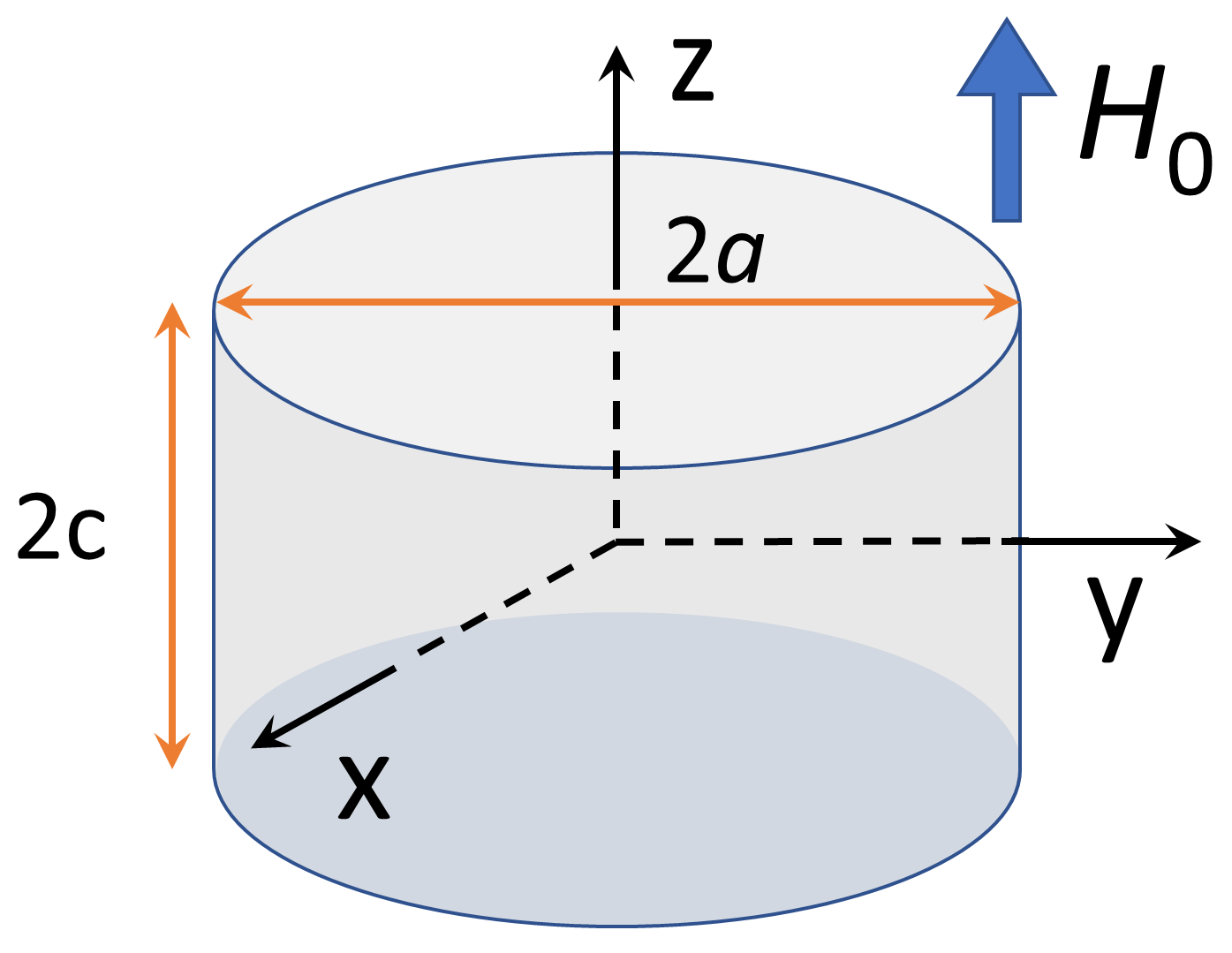
Figure 1: Geometry used in this paper: a right circular cylinder of radius $a$ and thickness $2c$ oriented as shown in a uniform axial magnetic field, $H_{0}$, produced by external sources.

Of course, real superconducting samples, especially single crystals, often have platelet shape with two parallel surfaces and polygonal in-plane cross-section, which varies from rectangles and prisms to triangles. It turns out, we can approximately map any such shape onto a cylinder by calculating the radius of an equivalent cylinder based on the volume penetrated by the magnetic field. For small $\lambda$, this volume is given by the surface area of crystal faces parallel to the magnetic field times $\lambda$. Of course, this simplification neglects top and bottom surfaces perpendicular to the field. However, for thin samples a renormalized London penetration depth can be introduced in the same manner. In other words, the penetrated volume is proportional to the product of sample thickness, penetration depth $\lambda$ and the perimeter, $P_{S\perp H}$, of the in-plane cross-section, perpendicular to the field. Therefore, one can map any cross-section shape onto a cylinder, using $P_{S\perp H}=2\pi a^{\prime}$, where $a^{\prime}$ is the radius of the “equivalent” cylinder. For example, often studied cuboidal sample with a rectangular cross-section, $2a\times 2b$, is mapped onto the equivalent right circular cylinder of radius,

$$a^{\prime}=\frac{2}{\pi}\left(a+b\right)$$ (1)

and of the same height, $2c$, along the magnetic field, as the original $2a\times 2b\times 2c$ cuboid. Therefore, there is a wide applicability of our results for quantitative calibration of the magnetic susceptibility, for example to extract the London penetration depth. The step-by-step procedures are described at the end of the paper.

I.2 The dimensionality of flux penetration

As a starting point, let us review some known analytical solutions of the London equations in different geometries paying attention to the effective dimensionality of flux penetration. For derivations, see the mathematically identical problem of the electric field polarization in conductors of various shapes solved as problems in Chapter VII of “Electrodynamics of Continuous Media”, by Landau and Lifshitz (vol. 8) [4]. Everywhere in this paper we assume isotropic superconductors.

An apparent measured magnetic susceptibility is defined as:

$$\chi=\frac{dM}{dH}=\frac{1}{V}\frac{dm}{dH}$$ (2)

where $M=m/V$ is volume magnetization, $m$ is the total magnetic moment and $V$ is the sample volume. Note that using volume-normalized $M$ does not imply spatially-uniform magnetization density. This magnetic susceptibility $\chi$ is defined only in the integral sense. For example, two samples of the same volume, but different shapes will produce two different values of $m$, therefore different $\chi$. A general discussion of the magnetic moment and its evaluation in arbitrary shaped samples is given elsewhere [2].

Let us introduce the dimensionality, $D$, of the magnetic field penetration into the specimen. This is not the geometric dimensionality of the sample itself (such as 1D wire, 2D film or 3D cube), but rather the dimensionality of the propagating magnetic flux front advancing into the sample. Assuming $\lambda\ll R$, the geometric interpretation of the magnetic susceptibility is that the value of an ideal diamagnet, $\chi=-1$, is reduced by the ratio of the volume penetrated by the magnetic field to the total volume of the sample:

$$\chi\left(1-N\right)\approx\frac{\Delta V}{V}-1$$ (3)

where $N$ is the demagnetizing factor, $V$ is sample volume and $\Delta V$ is the volume penetrated by the magnetic field. This equation follows trivially from the exact Eq.13 discussed below. Let us analyze three representative cases for which the analytic solutions of the London equation are known.

One-dimensional penetration of a magnetic field along the $x-$axis into a slab of width $2a$ and infinite in $y$ and $z$ directions. In this case we can think of a volume of a parallelepiped $L\times L\times\left(2a\right)$ with the side surface $L\times L$ parallel to the applied field. The penetrated volume is:

$$\Delta V=2\left(aL^{2}-\left(a-\lambda\right)L^{2}\right)=2aL^{2}\frac{\lambda}{a}=V\frac{\lambda}{a}$$

where a factor of $2$ in front comes from two surfaces located at $\pm a$. Here the dimensionality of flux penetration is determined by the term $\left(a-\lambda\right)$ in the first power resulting in $\chi\sim r$, therefore $D=1$. Equation 3 gives: $\chi=r-1$, where $r=\lambda/a$. Indeed, the exact solution is compatible with this small-$r$ limit [5],

$$\chi_{slab}\left(r\right)=r\tanh\frac{1}{r}-1$$ (4)

Two-dimensional penetration occurs in an infinite cylinder of radius $a$ in an axial magnetic field. Following the same logic as above we can write per length $L$ along the cylinder axis:

$$\Delta V=L\pi a^{2}-L\pi\left(a-\lambda\right)^{2}\approx 2V\frac{\lambda}{a}$$

where we only left first order in small parameter, $r=\lambda/a$, terms. Here the dimensionality of flux penetration is determined by the $\left(a-\lambda\right)^{2}$ term, so to the first order $\chi\sim 2r$, which implies $D=2$. The exact solution of the London equation for the infinite cylinder in an axial field is [4],

$$\chi_{cyl,axial}\left(r\right)=2r\frac{I_{1}\left(\frac{1}{r}\right)}{I_{0}\left(\frac{1}{r}\right)}-1$$ (5)

where $I_{\nu}\left(z\right)$ are the modified Bessel functions of the first kind. Indeed, it has a factor of 2 in front. It is interesting to note that the transverse magnetic field penetration into such cylinder has exactly the same functional form only adding a factor of $2=1/\left(1-N\right)$ from the demagnetizing factor, $N=1/2$ [4]:

$$\left(1-\frac{1}{2}\right)\chi_{cyl,perp}\left(r\right)=2r\frac{I_{1}\left(\frac{1}{r}\right)}{I_{0}\left(\frac{1}{r}\right)}-1$$ (6)

and the above arguments about $2D$ flux penetration hold in this case as well.

Three-dimensional flux penetration into a superconducting sphere of radius $a$ is accompanied by the penetrated volume:

$$\Delta V=\frac{4}{3}\pi a^{3}-\frac{4}{3}\pi\left(a-\lambda\right)^{3}\approx 3V\frac{\lambda}{a}$$

where we dropped all higher order terms in $r$. Here, following the same logic as above, the effective dimensionality is determined by the $\left(a-\lambda\right)^{3}$, giving $\chi\sim 3r$, which means $D=3$ in this case. Indeed, the exact solution for a sphere is [5],

$$\left(1-\frac{1}{3}\right)\chi\left(r\right)=3r\coth\frac{1}{r}-3r{{}^{2}}-1$$ (7)

Similar to the cylinder in transverse field, there is a pre-factor $\left(1-N\right)$ with $N=1/3$ in this case. In the first two cases of the infinite slab and cylinder, $N=0$. Clearly, the dimensionality, $D$, of the magnetic flux penetration and demagnetizing factor are not rigidly connected.

Figure 2(a) shows these analytic functions, Eqs.4-7, plotted on one graph revealing quite a substantial apparent difference at all values of $r$. Obviously, the difference is mostly due to different $D$, which determines the slope of $\chi\left(r\right)$ at small $r$. Therefore, it is convenient to re-scale the field penetration parameter $r$ to make the initial slope the same for all curves. In principle, any suitable function ($\tanh$ or Bessel functions) and any $D$ can be chosen, it is convenient to choose $D=2$ , because this is the most general case matching the dimensionality of the magnetic field itself. It penetrates general sample from two sides and is infinite in the third direction. Therefore we can write:

$$r=\frac{\lambda}{a}\rightarrow\frac{2}{D}\frac{\lambda}{a}$$ (8)

which modifies the infinite slab case to $r\rightarrow 2r$, leaves the $2D$ case unaffected, and changes the $3D$ case to $r\rightarrow 2r/3$.

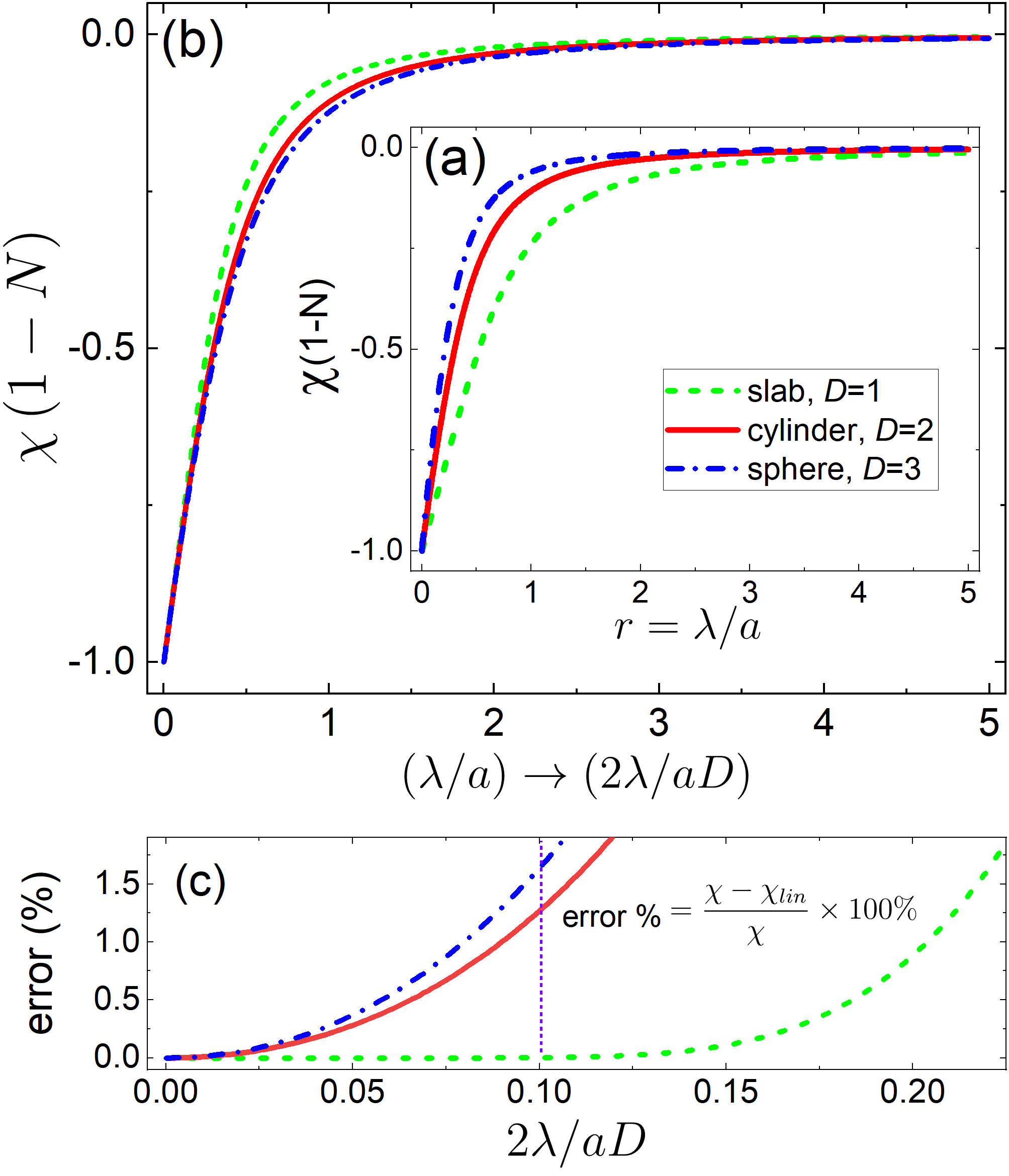
Figure 2: (a) (inset) Magnetic susceptibility of an infinite slab, an infinite cylinder (axial and perpendicular - the same curve) and of a sphere as function of $r=\lambda/R$; (b) the same curves, but in re-scaled penetration parameter, $r\rightarrow 2r/D$; (c) percentage deviation of the re-scaled curves of the full expressions, Eqs.4-7, from the linear form, Eq.9.

Figure 2(b) shows that the same curves become much closer to each other when plotted in re-scaled coordinates, Eq.8, and coincide (by design) at small values of $r$. In all cases, the initial susceptibility is apparently linear in $r=\lambda/R$ and can be written as:

$$\left(1-N\right)\chi_{lin}=D\frac{\lambda}{a}-1$$ (9)

The goal of this paper is to find numerical solutions for the magnetic susceptibility in finite right circular cylinders with rectangular cross-section and present it in the form similar to Eq.9, as

$$\left(1-N\right)\chi_{lin}=\frac{\lambda}{\eta a}-1$$ (10)

where all the effects of finite geometry and deviations from the ideal shape are absorbed in the effective demagnetizing factor, $N,$ and the response to the propagating magnetic flux, including the factor $D=2$, are reflected in the dimensionless function $\eta$, so that $R=\eta a$ can be viewed as the “effective” sample radius.

I.3 Magnitude of the London penetration depth

Before we proceed with the calculations, let us estimate at what values of $r$ the non-linearity caused by the hyperbolic functions become important. We calculate the percentage deviation as:

$$\textnormal{error}=\frac{\chi-\chi_{lin}}{\chi}\times 100\%$$ (11)

This quantity is shown in Fig.2(c) for all three cases. A quite conservative estimate is that the linear approximation, Eq.9, is good within 1% accuracy for $r\lesssim 0.1$. Let us translate this criterion into the real-world values. Consider a generic temperature-dependent London penetration depth, $\lambda\left(t\right)$=$\lambda\left(0\right)/\sqrt{1-t^{2}}$, where typical $\lambda\left(T=0\right)\lesssim 300\;\textnormal{nm}$, and typical $a\approx 500\;\mu\textnormal{m}$ for a mm - sized crystal. Here $t=T/T_{c}$ is the reduced temperature and $T_{c}$ is the superconductor transition temperature. Then the dimensionless ratio $r=0.1$ is reached at $t(r=0.1)=\sqrt{1-\left(\lambda\left(0\right)/0.1a\right)^{2}}=0.99998\approx 1-\left(2\times 10^{-5}\right)$. This is, indeed, experimentally negligible temperature distance from $T_{c}$. In fact, the range of realistically important values of $r$ is much less than $0.1.$ Even a simple estimate of a temperature at which $\lambda$ increases five fold, $\lambda\left(t_{5}\right)=5\lambda\left(0\right)$ gives $t_{5}=\sqrt{1-\left(1/5\right)^{2}}\approx 0.98$, which covers most of the superconducting domain, while this value corresponds to only $r=5\times 0.3/500=0.003$ where Eq.9 is definitely a very good approximation. Note that sometimes used two-fluid phenomenological function, $\lambda\left(t\right)=\lambda\left(0\right)/\sqrt{1-t^{4}},$gives estimates even closer to $T_{c}$. Therefore, we conclude that practically important values of $r$ are small and the linear approximation, Eq.9 is well justified in most practical situations. This also eliminates the problem of temperature-dependent demagnetizing factor (only for a superconductor!) and allows us to use the demagnetizing factor of an ideal diamagnetic sample of the same shape and volume as the sample under study.

In Section II.D we revisit these estimates, because the field penetration parameter can be significantly renormalized, especially in thinner samples. We find that even then linear approximation is applicable.

I.4 Numerical solution of the London equations in three dimensions

For numerical computations we use the AC/DC module of COMSOL 5.6 software [6] designed to solve the frequency-dependent Maxwell equations with proper boundary and initial conditions. Detailed description of the software and its capabilities can be found in the documentation [6]. Figure 3 (a) shows how the geometry of the sample, shown in Fig.1, is implemented in COMSOL. The Maxwell’s Ampère’s equation written for a material with pure imaginary electric conductivity,

$$\sigma=-\frac{i}{\mu_{0}\omega\lambda^{2}}$$ (12)

turns it into the London equation when we set the relative electric permittivity $\epsilon=0$. The critical step of the numerical analysis is the construction and optimization of the adaptive mesh that should be fine enough to resolve the exponential penetration of a magnetic field into a superconductor at distances smaller than the London penetration depth, $\lambda$, and it has to be done in a three-dimensional space. In case of a cylinder the 3D problem of a vector field, $\mathbf{B}=\left(B_{x},B_{y},B_{z}\right)$ can be mapped onto a 2D problem, $\left(B_{r},0,B_{z}\right)$, considering only one component of the vector potential in cylindrical coordinates is needed, $\mathbf{A}=\left(0,A\left(r,z\right),0\right)$. Still, full 3D distribution of the magnetic field is obtained numerically exploiting the axial symmetry of the problem. Figure 3(b) shows an example of the small part of the adaptive mesh cross-section, zooming onto a tiny area near the corner. The actual mesh is even much denser and this image would be completely black. In the calculations we used $a=100\;\mu\textnormal{m}$ and calculated $\lambda$ values starting from $0.1\;\mu\textnormal{m}$ to $500\;\mu\textnormal{m}$ which covers the realistic range of $\lambda$$\left(T\right)$ in typical superconductors. We also explored a difficult case of $c<\lambda$$\ll a$ in order to describe an important thin film limit.

To check the numerical results, different types of the adaptive mesh (e.g. tetrahedral or hexahedral) and its refinement strategies was attempted. Different sample and mesh sizes with and without boundary layers constructed. The reported finding are robust and independent on the particular choice of the mesh or algorithms. In all cases, the extrapolation of the results to the ideal diamagnet limit, $\lambda=0$, was checked for consistency. In that limit, a much simpler (and therefore easier to solve) magnetostatic problem of a linear magnetic material with $\chi=-1$, was calculated. This limit is explored elsewhere [2].

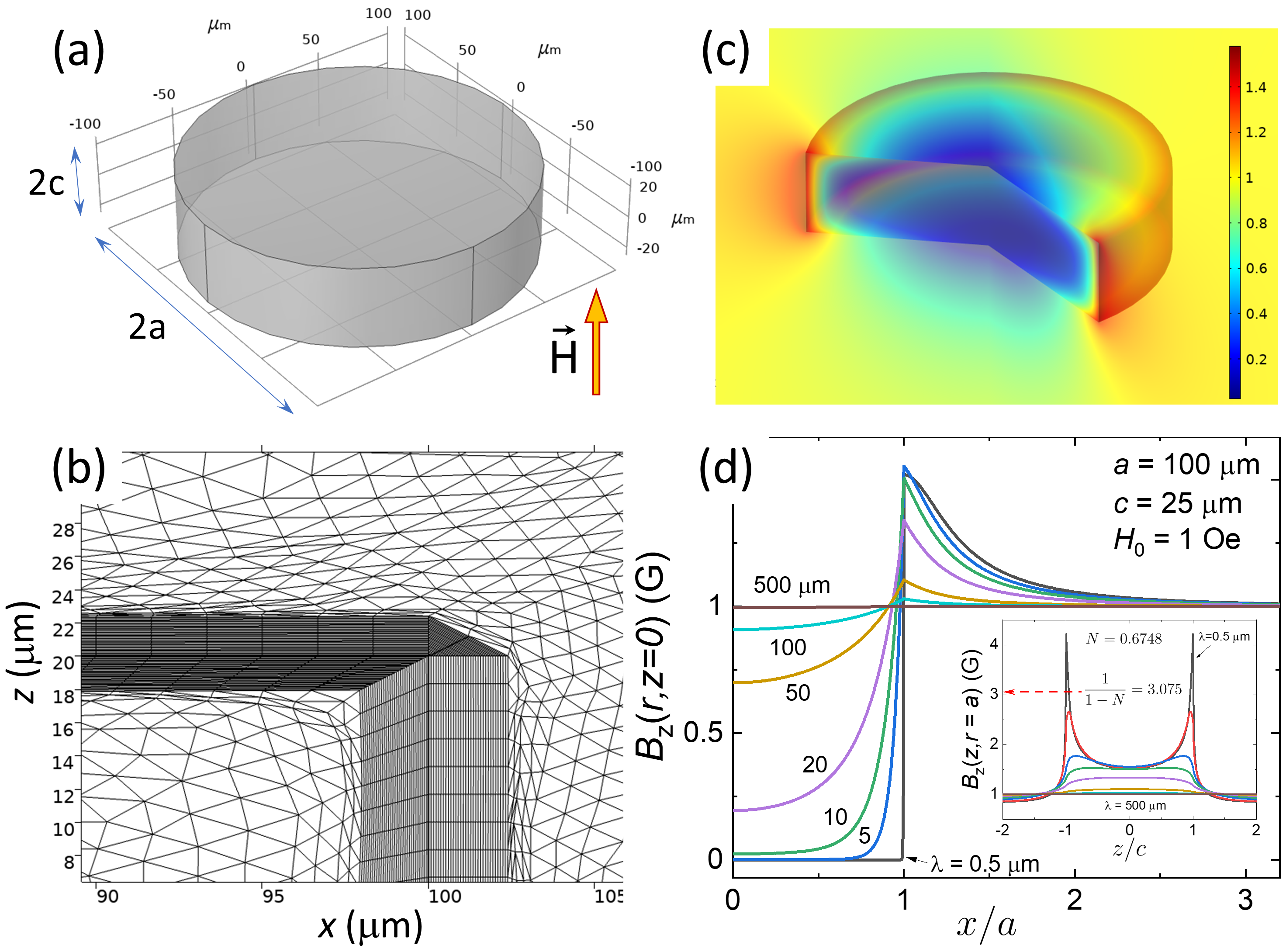
Figure 3: (a) Geometry defined in COMSOL with designation of dimensions used in this work. Compare to Fig.1. (b) Example of the adaptive mesh near the corner with mesh fine enough to resolve exponential flux distribution (note the axes scales in $\mu\textnormal{m}$); (c) COMSOL calculation example of the 3D distribution of the magnetic induction of a superconductor in an applied magnetic field, $H_{0}=1\;\textnormal{Oe}$, for a large $\lambda/a=0.2$ to make flux penetration visible. (d) Profiles of the $z-$component of the magnetic induction calculated for the sample with $a=100\;\mu\textnormal{m}$ and $c=25\;\mu\textnormal{m}$ at $\lambda=0.5,1,5,10,20,50,100,500\;\mu\textnormal{m}$. Main frame: $B_{z}(r)$ through the sample center, $z=0$; inset: $B_{z}(z)$ along the sample side, $r=a$.

Figure 3(c) shows an example of a calculated 3D distribution of the magnetic induction calculated for a particular aspect ratio, $\nu=c/a=25/100=0.25$, and the London penetration depth, $\lambda=20\;\mu\textnormal{m}$, in a static applied external magnetic field of $H_{0}=1\;\textnormal{Oe}$. Figure 3(d) shows the magnetic induction profiles calculated for the indicated values of $\lambda$. The main frame shows a radial distribution, $B_{z}\left(r\right)$, from the sample center at $z=0$, and the inset shows $B_{z}\left(z\right)$ along the sample side, at $r=a$, for the same set of $\lambda$. Note a very strong variation of the magnetic field along the surface invalidating any attempt to use the “average” demagnetizing field to map this onto an ellipsoid where this field is constant, $H=H_{0}\left(1-N\right)$.

II Results and discussion

II.1 The effective demagnetizing factor, $N$

The effective demagnetizing factor, $N$, in arbitrary-shaped samples, including finite cylinders, was discussed in detail elsewhere [2]. Here we review the results of these calculations and provide more detailed formulas for specific cylindrical geometry considered here to be used when constructing the quantity, $\chi\left(1-N\right)$ from the experimental data. There are several ways to introduce $N$ in non-ellipsoidal bodies. The total magnetic field experienced by the sample includes the demagnetizing field, $H_{total}=H_{0}+H_{d}$. In a uniformly magnetized ellipsoid with constant demagnetizing factor $N$, this field is also uniform, $H_{d}=-NM$, where $M$ is constant volume magnetization. Inspired by this general picture, different authors used various numerical, empirical and analytical methods to evaluate $\mathbf{H}_{d}\left(\mathbf{r}\right)$ and $\mathbf{M\left(r\right)}$, which are no longer uniform in the non-ellipsoidal samples, see Fig.3(d).

In this paper we calculate the total magnetic moment, $m$, in the direction of the applied magnetic field, which is only straightforward in the case of free currents of known distribution. However, it is also possible to calculate $m$ integrating the known distribution of $B_{z}\left(r\right)$, which is relatively simple numerically, but its proof in general samples is non-trivial Ref.[7, 2]. The magnetic moment (and an apparent “integral” magnetic susceptibility are given by):

$$\mathbf{m}=\alpha\intop_{V}\left(\frac{\mathbf{B}\left(\mathbf{r}\right)}{\mu_{0}}-\mathbf{H_{0}}\right)d^{3}\mathbf{r}=\chi\mathbf{H_{0}}V$$ (13)

where the coefficient $\alpha=3/2$ for the integration over the large spherical domain that includes the whole sample, whereas $\alpha=1$ is for the integration domain as a large cylinder with its axis parallel to $\mathbf{H_{0}}$. (Yes, the integral depends on the way it is evaluated! Mathematically, this is similar to finding an electric field in a uniformly charged space [2]). Then, using the definition:

$$\chi=\frac{\chi_{0}}{1+N\chi_{0}}$$ (14)

the effective (integral) demagnetizing factor is defined as,

$$N=\frac{1}{\chi}-\frac{1}{\chi_{0}}$$ (15)

where $-1\leq\chi_{0}\leq\infty$ is the material’s intrinsic magnetic susceptibility (in a sample without demagnetization). In the case of a perfect superconductor (perfect diamagnet), $\chi_{0}=-1$ and

$$N=\frac{1}{\chi}+1$$ (16)

It should be noted that historically, two effective demagnetizing factors were introduced: $N_{m,f}=\left\langle H_{d}\right\rangle_{V,S}/\left\langle M\right\rangle$_V,S, were index $V$ is for the volume averaging, and index $S$ is for the averaging of these quantities in the middle plane perpendicular to the field. The first kind is called the “magnetometric” factor, $N_{m}$, and the second is called the “fluxmetric” (or “ballistic”) demagnetizing factor, $N_{f}$, respectively. Yet another approach is to use the total magnetostatic energy, $NM^{2}/2\mu_{0}$, which can be calculated numerically [8]. With three possible orthogonal orientations of the magnetic field, along $x,y,z$, three principal demagnetizing factors are defined. Detailed calculations in finite cylinders with rectangular cross-section are given in Refs.[9, 1]. Chen, Brug, and Goldfarb give a comprehensive discussion with many references to the prior works [1]. Unfortunately, perhaps due to the intricacy of the expressions of the spatial distributions, most works also assume that the sum of the three demagnetizing factors in three principal directions, $\sum_{i}N_{i}\equiv N_{x}+N_{y}+N_{z}=1$. However, this is only true for the ellipsoidal shapes where the magnetic induction (therefore local susceptibility $\chi$) inside the sample is constant and uniform. This condition does not hold for the generalized effective demagnetizing factors, as followed from works that did not use this assumption [9, 1, 2]. The actual variation of the magnetic field in finite samples is highly non-uniform (see, e.g., Fig.3(d)), which makes the fluxmetric factor to be a very poor approach in general. With the mentioned assumption, $\sum N_{i}=1$, the magnetometric factor is also incorrect.

As a particular case, let us compare the effective demagnetizing factor of a perfectly diamagnetic circular cylinder of radius $a$ with the square cross-section in the $r-z$ plane, $2a\times 2a$, in the axial magnetic field along the $z$ axis. Our numerical result is $N=0.36569$ [2], identical value of the best fit, Eq.18, and almost the same $N=0.36576$ from what we call a “practical” fit, Eq.19. This has to be compared with $N=0.36482$ given by Brandt [10] and $N=0.3692$ by Taylor [9], apparently showing an excellent agreement between these studies. Furthermore, for the sum, Taylor finds: $N_{z}+2N_{x,y}=0.3692+2\times 0.3669=1.103>1$, in agreement with our result, $\sum N_{i}=0.36569+2\times 0.36673=1.100$. In a stark contrast, the works that do use the $\sum N_{i}=1$ assumption underestimate the demagnetizing factor, for example Sato et al. report $N_{z}=0.307054$ [8] and Arrott et al. give $N=0.311577$ [11]. The fluxmetric (ballistic) factors are much lower due to the significant underestimate of the demagnetizing field evaluated only in the middle plane where it is the smallest, e.g., Joseph et al. report $N=0.2322$ [12]. This if not unique to cylinders. For example, for a cube along three principal directions, $N_{x}=N_{y}=N_{z}=0.38919$ from our work [2] and $N=0.389667$ calculated by Pardo, Chen and Sanchez [13] showing excellent agreement despite the fact that they used quite different numerical methods. And, indeed, the sum is $\sum N_{i}=3\times 0.38919=1.1676>1$, notably exceeding 1.

II.2 Demagnetizing factor of a right circular cylinder in an axial magnetic field

Unlike the magnetometric factor mentioned above, most often used in literature, the demagnetizing factor used here involves the actual value of the applied field, not the average at the sample location quantity. This uniform magnetic field is set by the external sources far from the sample. Of many previous works, it turns out that Ernst H. Brandt has correctly calculated $N$ in this case for arbitrary aspect ratio [10]. His approximate expression for a cylinder in an axial magnetic field is:

$$\frac{1}{N}=1+\frac{3\pi\nu}{4+2\tanh\left[1.27\nu\ln\left(1+\nu^{-1}\right)\right]}$$ (17)

where $\nu=c/a$ is the aspect ratio. Figure 4 shows $N$ evaluated numerically using Eqs.13,16 in comparison with approximate expressions. Brandt’s Eq.17, shows an excellent agreement with our numerical results. This, in turn, lends further support to our calculations considering Brand’s considerable expertise in theoretical superconductivity, in particular dealing with finite size non-ellipsoidal samples. Brandt has also noted that $\sum N_{i}\neq 1$ for non ellipsoidal shapes.

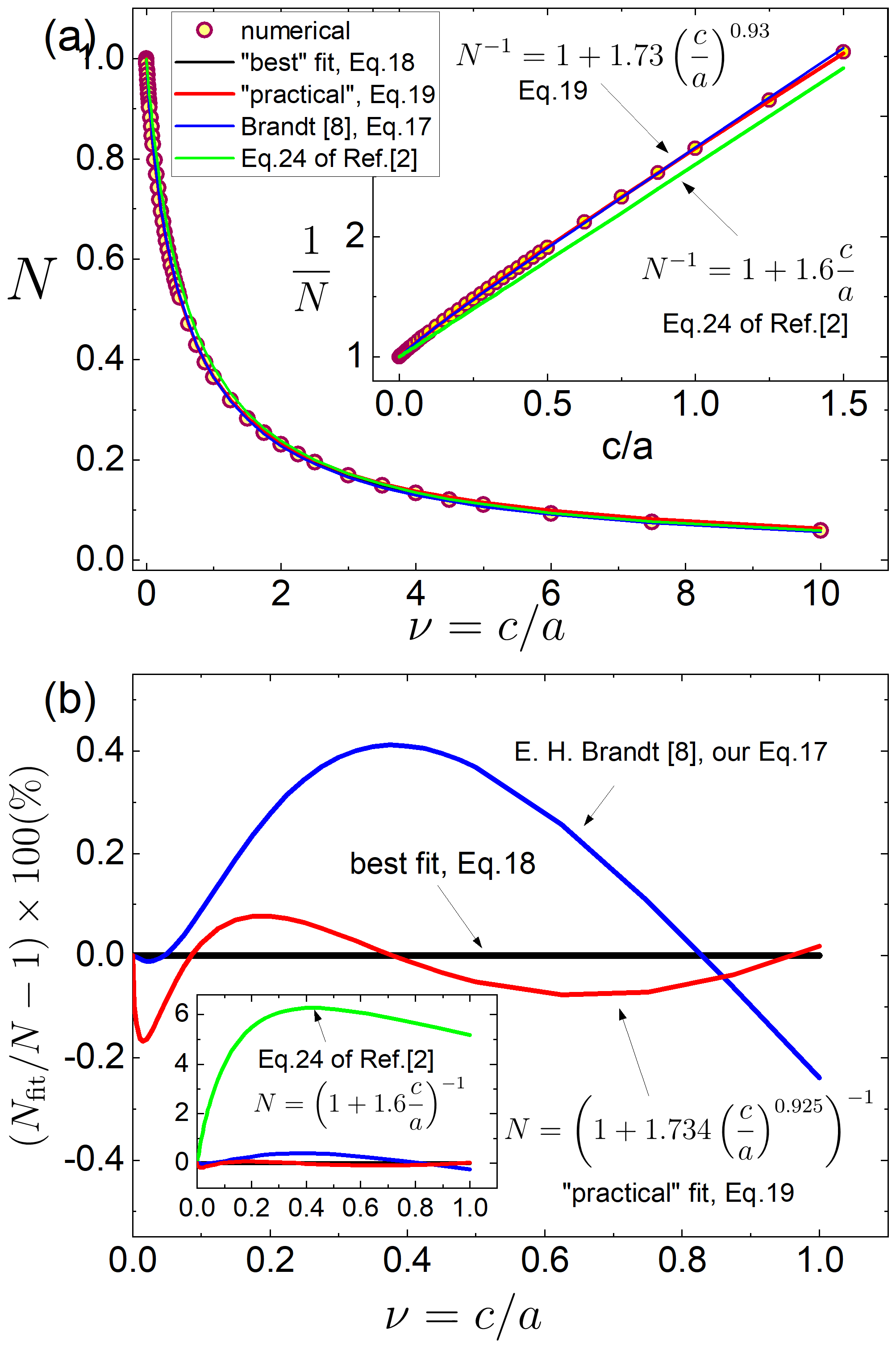
Figure 4: (a) Effective demagnetizing factor, $N$, as function of the aspect ratio, $\nu=c/a$. Symbols are the numerical results from our early work [2] and solid lines are the fits. The black solid line labeled “best fit” is Eq.18, red line “practical fit” is Eq.19 and blue line is Brand’s result, Eq.17. For comparison, a simplified curve where $1/N$ is a linear function of $\nu$ is shown by the green line, Eq.24 of Ref.[2]. (b): The percent deviation of these fitting curves from the numerical data. The inset shows a much larger deviation when linear approximation for $1/N$ is included.

To find easy to use functional form, we used TableCurve2D software that fits a given set of data points to dozens of different functions and ranks them by type and goodness of fit criterion. The best not too complicated fit of our numerical results for all values of $\nu$ is given by:

$$N=\frac{a+c\nu^{0.5}+e\nu+g\nu^{1.5}+i\nu^{2}}{1+b\nu^{0.5}+d\nu+f\nu^{1.5}+h\nu^{2}}$$ (18)

with the coefficients:

$a=$	$0.999999949328650188$
$b=$	$3.36894653579048123$
$c=$	$3.36942413926991188$
$d=$	$8.32140656517217575$
$e=$	$5.94222295811372722$
$f=$	$7.0090557033581253$
$g=$	$-0.363915848221631658$
$h=$	$7.5967537756996193$
$i=$	$0.034309628991176873$

Figure 4(b) shows the percentage deviation between the fit and the numerical results. The black curve labeled “best fit” showing a perfect agreement in the whole range from ultra-thin limit to long cylinders. Equation 18 is the most accurate choice for numerical work. However, a much simpler and concise (red curve labeled “practical”) fit also shows an agreement better that $0.2\%$ in the whole range,

$$N=\frac{1}{1+1.73401\nu^{0.92505}}$$ (19)

II.3 Magnetic susceptibility of finite right circular cylinders in an axial magnetic field

The next task is to calculate numerically the apparent magnetic susceptibility defined by Eq.2. For each value of the ratio, $\nu=c/a$, the magnetic induction distribution, $\mathbf{B}\left(\mathbf{r}\right)$, in the sample and space outside is calculated for a wide range of different values of the London penetration depth (see, for example, Fig.3(c) and d)), including the thin film limit of $c<\lambda\left(0\right)\ll a$ as well as long samples up to $c/a=2.5$. Then Eq.13 was used to obtain the total magnetic moment, $m$, from which the effective demagnetizing factor was calculated using Eq.16. It is important that we do have a perfect diamagnet limit, $\lambda=0$, from the solutions for the demagnetizing factor [2]. Therefore, we could verify that the calculated curves $\chi\left(r=\lambda/a\right)$, indeed, extrapolate to the value of $1/\left(1-N\right)$ for $r\rightarrow 0$ Therefore, all curves plotted as $\chi\left(1-N\right)$ start from the same value of $-1$. For convenience of presentation, we start from zero by plotting $\chi\left(1-N\right)+1$ in Fig.5. Each curve shows magnetic susceptibility vs. the ratio of $\lambda/a$ in the interval from $0$ to $2.5$. Each curve is calculated for a given aspect ratio, $\nu=c/a$, forty two curves total covering all practically reasonable values from very thin to a very thick limit.

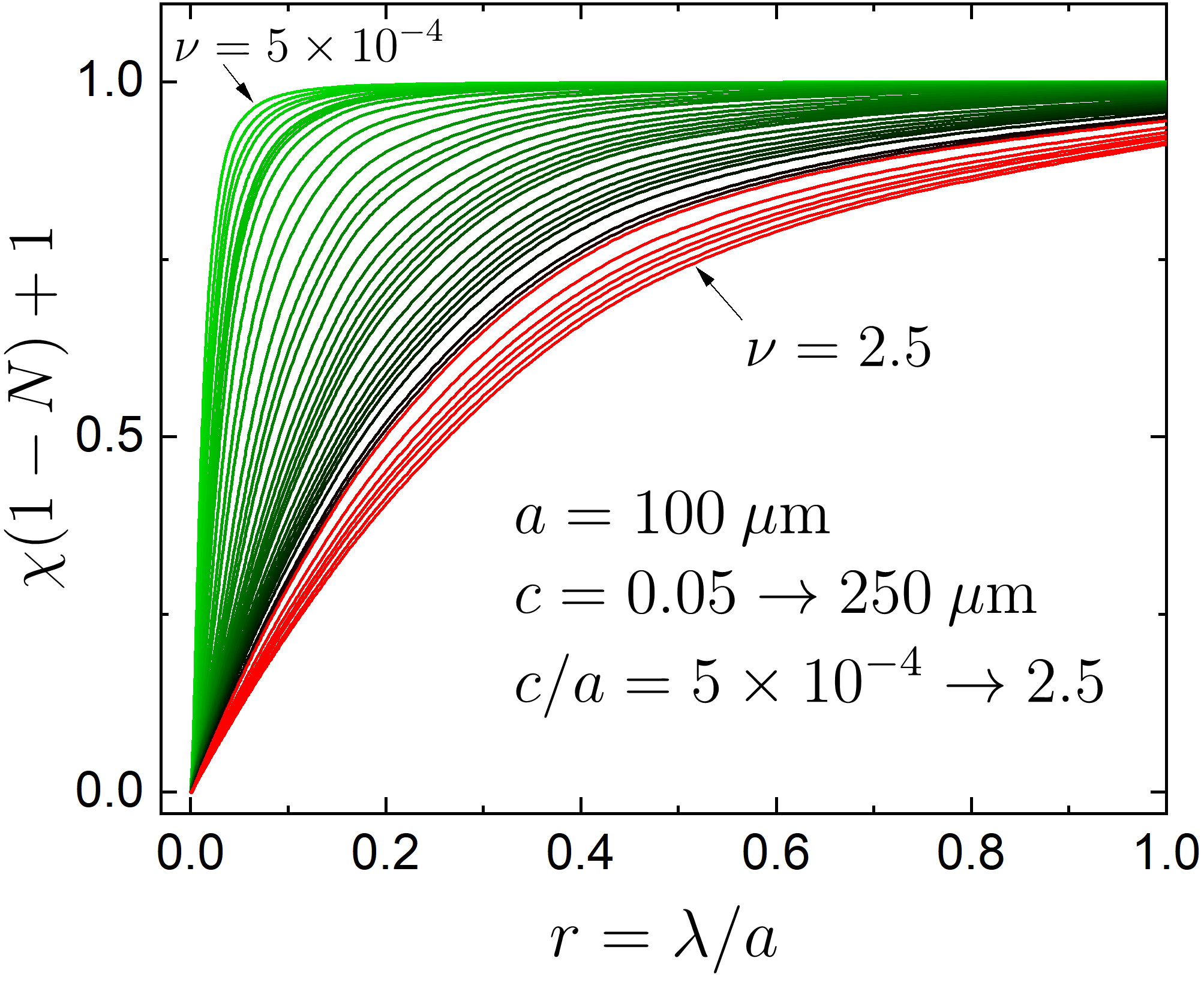
Figure 5: Calculated magnetic susceptibility of finite cylinders in axial magnetic field. Plotted is $\chi\left(1-N\right)+1$ versus the ratio $\lambda/a$. Each curve is calculated for a specific aspect ratio, $\nu=c/a$ raging from $\nu=5\times 10^{-5}$ to $\nu=2.5$, - forty two curves in total.

We note that the alternative description would be to include the finite-$\lambda$ dependence in the demagnetizing factor, $N\left(\lambda\right)$, defined from the general Eq.15. However, we prefer to separate the ideal demagnetizing factor, $N$, which depends only on the sample shape from the characteristic field-penetration parameter, $\eta\left(\nu\right)$, discussed in the next section. The problem is that at large values of $\lambda/a$ the equations become non-linear, instead of Eqs.4-7. Yet we can keep using constant $\chi-$independent $N$ and push all the correction to this parameter $\eta\left(\nu\right)$. Here we introduce the geometric correction factor, $\eta\left(\nu\right)$, that re-normalizes the $\lambda/a$ parameter depending on the sample geometry.

II.4 The geometric correction factor, $\eta\left(\nu\right)$

As a next step, the initial susceptibility, the slope of each curve in Fig.5 was fitted to Eq.9 to obtain the geometric correction coefficient, $\eta\left(\nu\right)$, that is used to remap all the curves to one with a common initial slope. The dimensionality of flux penetration was fixed to $D=2$ to ensure the correct infinitely-long cylinder limit, $\eta\left(\infty\right)=0.5$. The red solid curve in Fig.6 corresponds to the best fit, Eq.20. The symbols are the fitted data points. The simplified fit, Eq.22, is not shown in the main panel as it is hard to see behind the curves, but it practically coincides with the best fit. The discrepancy between the fits and the numerical results, $\textnormal{error}\;\%=\left(1-\eta_{\textnormal{fit}}/\eta\right)\times 100\%$, is plotted in the inset. For comparison with the previous results, the green dashed curve shows $\eta\left(\nu\right)$ suggested by us 21 years ago based on the specific analytical approximation of the spatial distribution of the magnetic induction on the sample surface (Eq.(2) of Ref.[3]) inspired by the projection of an ellipsoid onto a plane and calculating the expelled volume resulting in Eq.(6) in Ref.[3]. Back then we did not look at the thinner samples and, as a result, the suggested formula does not work at all below roughly $\nu<0.05$. Nevertheless, as can be seen in Fig.6, the dashed green curve is quite close to our new calculations approximately in the interval from $c/a=0.05$ to $0.5$. Fortunately, it covers the most practical range of experimental aspect ratios. For example, for a typical crystal of $1$ mm in diameter, the thicknesses from $50$ to $500\;\mu\textnormal{m}$ are described fairly well by Eq.(6) of Ref.[3] and these values are commonly used in the experiment. Importantly, the Eq.(6) of Ref.[3] was used extensively for the calibration of the magnetic susceptibility from sensitive frequency-domain measurements [14, 15]. In the thin limit, the previous estimate is wrong and it is important to correct that. Instead of a predicted saturation at $\eta$$\left(0\right)$=0.2, the correct curves decreases rapidly towards zero.

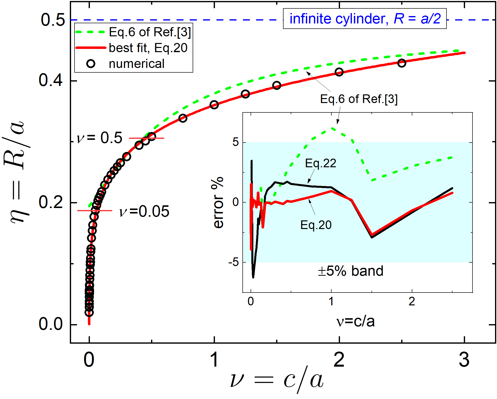
Figure 6: The geometric correction coefficient, $\eta\left(\nu\right)$ as function of the cylinder aspect ratio, $\nu=c/a$, calculated by fitting the initial slope of $\chi\left(\lambda/R\right)$ (see Fig.5) to Eq.9 with $D=2$. The solid red line shows our best fit, Eq.20 and the green line shows the plot of Eq.(6) of Ref[3]. It works not too bad in some most useful range of aspect ratios, from from approximately $c/a=0.05$ to $0.5$. The thin limit, though is wrong and it is important to correct that. The simplified fit, Eq.22, is not shown in the main panel as it is hard to see behind the curves, but it works very well as can be seen from the inset. The inset shows the relative error between the fits and the numerical data, $error\;\%=\left(\eta_{fit}/\eta-1\right)\times 100\%$. The red curve corresponds to the best fit, Eq.20. and black curve to Eq.22.

The calculated geometric correction factor, $\eta$$\left(\nu\right)$, can be well represented by the following numerical approximation (solid red curve in Fig.6):

$$\eta\left(\nu=\frac{c}{a}\right)=\frac{a+c\nu^{0.5}+e\nu+g\nu^{1.5}+i\nu^{2}}{1+b\nu^{0.5}+d\nu+f\nu^{1.5}+h\nu^{2}+j\nu^{2.5}}$$ (20)

with the coefficients:

$a=$	$-0.0281027472950638618$
$b=$	$4.58797296004528776$
$c=$	$2.875513314557569$
$d=$	$-137.801329718142642$
$e=$	$-33.7758403444390059$
$f=$	$1249.78954939821191$
$g=$	$188.948638333931676$
$h=$	$-123.317937748885354$
$i=$	$250.500066383141833$
$j=$	$138.717299394700242$

Please note, that while this equation provides a very good approximation of the calculated numerical values, it is only applicable in the calculated range of $\nu\leq 3$, which in practice covers all aspect ratios of experimental importance. At $\nu=3,$ Eq.22 gives, $\eta\left(3\right)=0.43963288651773$ while the terminal value at $\nu\rightarrow\infty$ should be $\eta\left(\infty\right)=0.5$, marked by the blue dashed line in Fig.6. For a smooth extrapolation that is valid for all values of $v$ we use Eq.20 for $\nu\leq 3$ and for $\nu>3$:

$$\eta\left(\nu\right)=0.5-\frac{0.18110134044681}{\nu}$$ (21)

We also found the simpler fitting function that works quite well for $\nu\leq 3$ :

$$\eta\left(\nu\right)=(a+b\ln\nu)^{2}$$ (22)

where the coefficients are:

$a=$	$0.6013634241567849$
$b=$	$0.05987611403976185$

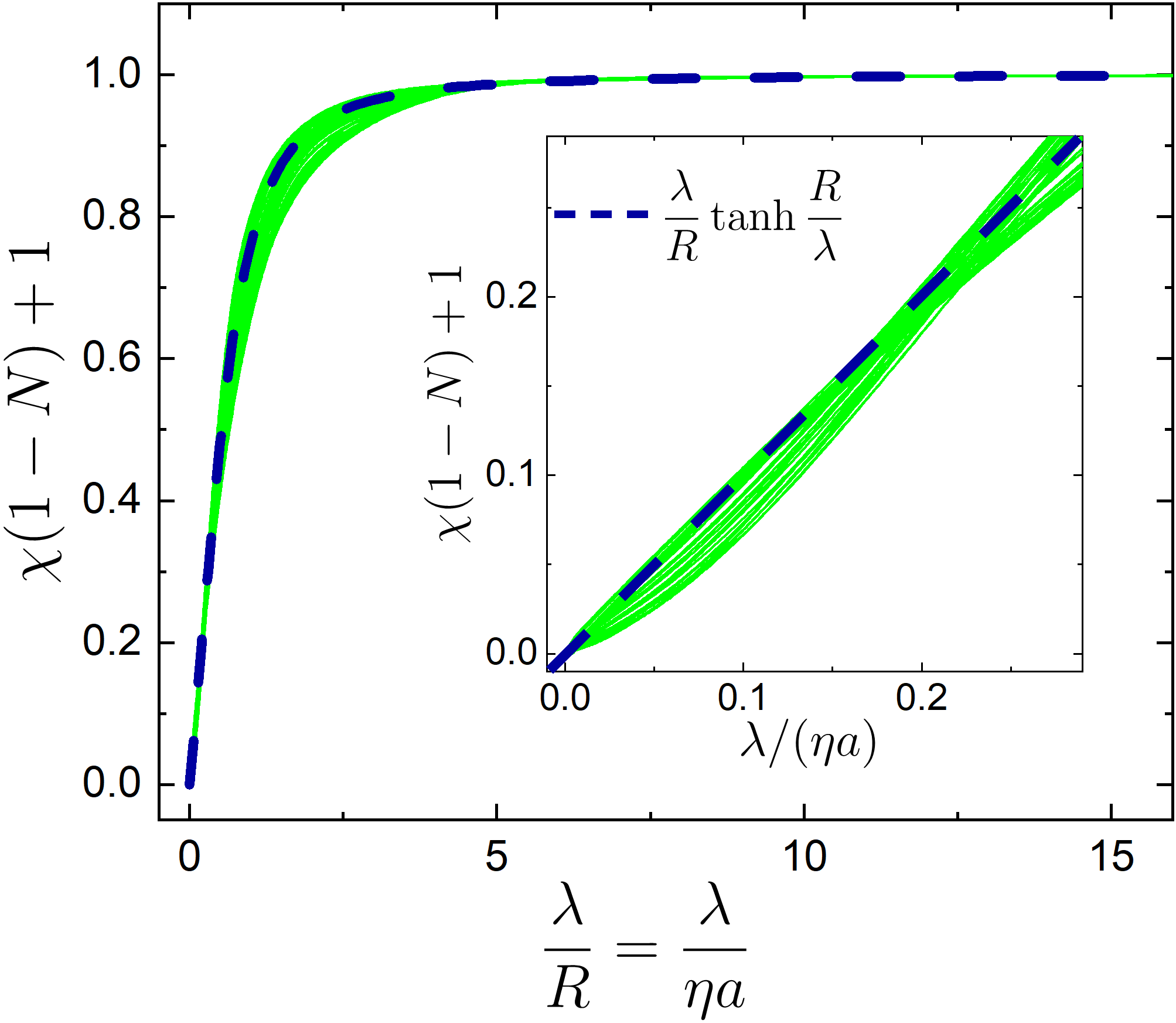
Figure 7: Scaled magnetic susceptibility, $\chi\left(1-N\right)+1$, plotted versus the scaled magnetic field penetration ratio, $\lambda/R=\lambda/\left(\eta a\right)$. Main frame is the full range and the inset shows the linear part. There are forty two curves plotted together showing the generally good trend towards the scaled behavior.

We can now use the calculated geometric correction factor, $\eta$$\left(\nu\right)$, and the demagnetizing factor, $N\left(\nu\right)$, to plot the scaled susceptibility, $\chi\left(1-N\right)$ versus the scaled field penetration ratio, $\lambda/R=\lambda/\left(\eta a\right)$. This is shown in Fig.7. Note the large expansion of this parameter range in thin samples while the calculations were done only up to $\lambda/a=2.5$. The dashed dark blue line shows analytical $\lambda/R\tanh\left(R/\lambda\right)$ function. Clearly, the scaled curves are clustered around it at all values and approach a single slope for small $\nu$. This region is zoomed at in the inset. Of course, the deviations are expected for the thinner samples due to both, technical and geometrical reasons. Technically it is difficult to build a good fine adaptive mesh in very narrow domains and, physically, the response changes when thickness becomes comparable to the London penetration depth. In fact, we can now revisit the regime of the linear behavior, Eq.9. We found above that linear approximation is applicable for up to $r\leq 0.1$. Now we need to apply it to the re-normalized quantity, $\lambda/\left(\eta a\right)\leq 0.1$. This places the upper limit on the penetration depth, $\lambda\leq 0.1\eta a$, which gives a hard cutoff when the smallest value, $\lambda\left(0\right)$, is used. With the same parameters as before, $\eta=\lambda/0.1a=0.3/\left(0.1\times 500\right)=0.006$, which is achieved at $\nu=1\times 10^{4}$ or $c=50$ nm for a 1 mm sized sample. This is a very thin film limit and clearly, our effective approach used here is no longer applicable. Perhaps, this is a good way to define an ultra-thin limit. Still, it also means that our approximation is valid in a wide domain of practical aspect ratios.

There is another way to analyze our results along the lines discussed at the end of Section II.B. Note that both, demagnetizing factor, $0\leq N\leq 1$, and the geometric correction coefficient, $0\leq\eta\leq 0.5$, are limited to the indicated intervals while the aspect ratio, $v=c/a\geq 0$ does not have an upper bound. Therefore, we can examine the function, $\eta\left(N\right)$ and see whether it has some simple representations and trends. Figure 8 shows the numerical results along with three approximations. Apparently, $\eta\left(N\right)$ is linear in the interval, $0\leq N\leq 0.93$. The best linear fit is $\eta\left(N\right)=0.5-0.34664N$ and, obviously, the simplest possible interpolation is:

$$\eta\left(N\right)=\frac{1}{2}-\frac{N}{3},\;\textnormal{for\;}0\leq N\leq 0.93$$ (23)

The whole curve is described reasonably well by the function:

$$\eta\left(N\right)=\frac{a+cN+eN^{2}}{1+bN+dN^{2}}$$ (24)

with the coefficients:

$a=$	$0.504378594750316222$
$b=$	$-0.517078267930805991$
$c=$	$-0.709566812021391927$
$d=$	$-0.446415444537349392$
$e=$	$0.205676653892788686$

It will be interesting to perform similar calculations for different geometries and see whether Eq.24 will show some universality or not.

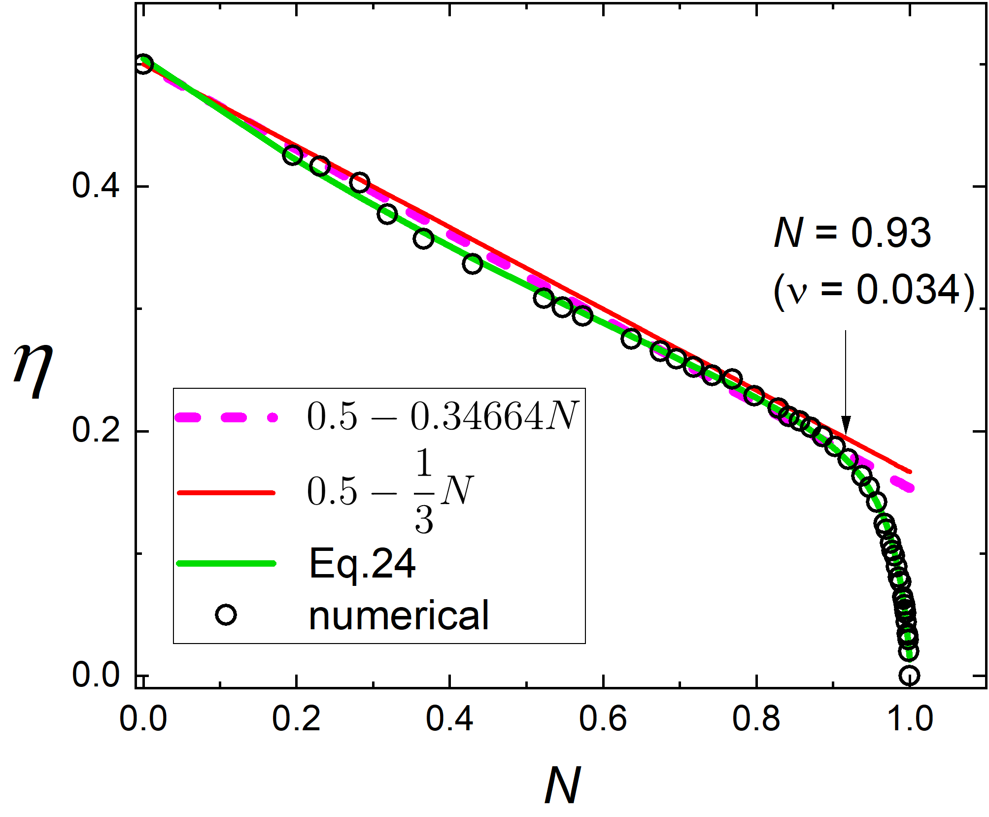
Figure 8: Geometric correction coefficient, $\eta$, as function of the demagnetizing factor, $N$. Symbols are the numerical results, dashed magenta line is the best linear fit and the red line is simple approximation, $\eta=\frac{1}{2}-\frac{N}{3}$ in the interval $0\leq N\leq 0.93$. The green curve is the reasonable fit valid at all values of $N$, see Eq.24.

III examples of practical applications

The obtained numerical results and analytical approximations can be used for general calibration of precision magnetic susceptibility measurements. Here we give two examples of practical applications.

III.1 Finding $N$ and $\eta$ without direct measurements of sample dimensions

The important utility of Eq.24 is that it gives the simple connection between $N$ and $\eta$, bypassing the need to figure out the exact dimensions of the crystal. Considering realistic shapes, calculating volume, $V$, from sample dimensions is no trivial task. On the other hand $V$ can be often estimated from the weight far more accurately than from the direct size measurements. (Material density is usually known at least from the parameters of the unit cell in crystals). Then, at the lowest temperature (as close to $\chi_{0}=-1$ as possible), one can use SQUID (or any other sensitive) magnetometer to measure the total magnetic moment, $m$, in an external magnetic field, $H_{0}$. Assuming perfect diamagnetism (which is quite accurate already below $0.98T_{c}$ as described in the introduction), the demagnetizing factor can be estimated from Eq.13 and Eq.14,

$$N=\frac{VH_{0}}{m}+1$$ (25)

Now using Eq.24 the geometric correction factor $\eta$ can be calculated. These two numbers, $N$ and $\eta$ are unique for each sample and they allow for a complete quantitative description of the magnetic properties in the Meissner-London state. Indeed, one can check the result by evaluating $N$ and $\eta$ using sample dimensions and compare the result. Whether Eq.24 has some universality or scaling in different shapes remains to be seen. It requires conducting similar calculations for other shapes, for example cuboids. If we compare demagnetizing factor for a cube, $N_{cube}\left(\nu=1\right)=0.38919$ with the demagnetizing factor for a cylinder with square cross-section, $N_{cylinder}\left(\nu=1\right)=0.36569$ they are both greater than that of a spheroid (sphere in this case) $N_{sphere}=1/3$, but the limiting case of all three for infinite $v$ is the same, $N_{\infty}=0$. For the cylinder with the square cross-section, $\eta_{cylinder}\left(\nu=1\right)=0.35714$ and for the sphere, by the definition of the re-scaling discussed in Section I.A, $\eta_{sphere}\left(\nu=1\right)=2/3=0.6(6)$, and therefore, it is more likely that the curves are different for each geometry. However, it is still possible that these curves for different shapes will only differ by a simple factor, because the general form of Fig.8 will be similar due to the bounds of $N$ and $\eta$.

III.2 Measurements of the London penetration depth

Suppose some quantity, $f,$ proportional to the magnetic susceptibility is measured. This can be the frequency of a tunnel-diode resonator or of a resonant microwave cavity, or the AC voltage of a sensitive susceptometer or, the DC voltage of a SQUID circuit with flux transformer. When a sample is inserted into the coil that provides an excitation magnetic field, $H_{0},$ (AC or DC depending on the method) small enough to stay in the Meissner state (no Abrikosov vortices), the measured quantity changes by some amount, $\varDelta f$. The maximum possible change, $\varDelta f_{0}$, is induced when an ideal diamagnet $(\lambda=0)$ of the sample size and shape is inserted. Therefore, the actual magnetic susceptibility is

$$\left(1-N\right)\chi=-\frac{\varDelta f}{\varDelta f_{0}}=\frac{\lambda}{R}-1$$ (26)

where the effective sample dimension, $R=\eta\left(\nu\right)a$. The quantity $\varDelta f_{0}$ can be measured directly by pulling the sample out of the coil at the base temperature. (Yes, one of our cryostats is equipped with a mechanical pulley of a spring-loaded sample holder, thus we can measure $\varDelta f_{0}$ directly and compare with the calculations). Alternatively, it can be calculated using the demagnetization factor described above. For example, in the case of a resonant circuit frequency shift,

$$\varDelta f_{0}=\frac{f_{0}V}{2V_{c}\left(1-N\right)}$$ (27)

where $V$ is sample volume and $V_{c}$ is volume of the coil. See Refs.[3, 16] for detailed discussion and derivation of Eqs.26 and 27. Now one can use Eq.18 or 19 to calculate $\varDelta f_{0}$. The next step is to extract the London penetration depth, $\lambda$, which is the final goal of this calibration procedure. In reality, the uncertainty of macroscopic dimensions compared to $\lambda$ is so large that it is only possible to precisely measure the relative changes with respect to the base temperature value, roughly speaking $\varDelta\lambda=\lambda\left(T\right)-\lambda\left(0\right)$, see detailed discussion in Ref.[16]. In other words, Eq.26 becomes:

$$\delta f\left(T\right)\equiv\varDelta f\left(T\right)-\varDelta f_{0}=\varDelta f_{0}\frac{\varDelta\lambda\left(T\right)}{R}$$ (28)

The measured quantity, $\delta\left(T\right)$ now gives the change in the London penetration depth,

$$\varDelta\lambda\left(T\right)=\frac{R}{\varDelta f_{0}}\delta f\left(T\right)=G\delta f\left(T\right)$$ (29)

where $R=\eta\left(\nu\right)a$ is the effective sample dimension calculated from Eq.20 (or approximately from Eq.22). For example, in the case of a tunnel-diode resonator, $f_{0}\sim 10\;\textnormal{MHz},$$\varDelta f_{0}\sim 5\;\textnormal{kHz}$ for typical sub-mm sized crystals with $R\sim 100\;\mu\textnormal{m}$. This gives the calibration constant $G=R/\varDelta f_{0}\sim 20\;\textnormal{nm}/\textnormal{Hz}$. The smallest frequency changes practically detected are about $\delta f\sim 0.02\;\textnormal{Hz}$ (giving $2$ parts per $10^{9}$ sensitivity of this technique!) resulting in resolving $\varDelta\lambda\left(T\right)\sim 0.4\;\textnormal{\AA}$ which is small enough to study the anisotropy of the superconducting gap [14, 15]. The full London penetration depth requires another measurement of the absolute value at least at one temperature [16].

IV Conclusions

In conclusion, a systematic quantitative description of the magnetic susceptibility of superconducting right circular cylinders of arbitrary aspect ratio, $\nu=c/a$, in an axial magnetic field is outlined for finite London penetration depth. It includes two independently computed quantities. (1) The demagnetizing factor, $N\left(\nu\right)$, of the ideal diamagnetic sample of the same shape and volume as the sample of interest and (2) the geometric correction factor, $0\leq\eta\left(\nu\right)\leq 0.5$, which takes into account the penetration of the magnetic field from all sides, including top and bottom surfaces, thus effectively reducing the relevant effective dimension, $R=\eta\left(\nu\right)a$, where $a$ is the radius of the cylinder. A simple connection between $N$ and $\eta$ valid for not too thin samples, $\nu\gtrsim 0.03$, is given by: $\eta\left(N\right)=0.5-N/3$. It may be helpful for a quick estimate of the geometric factor determining the effective flux penetration. With these quantities, the universal magnetic susceptibility is given approximately by:

$$\left(1-N\right)\chi=\frac{\lambda}{R}\tanh\frac{R}{\lambda}-1$$ (30)

The developed approach can be used for the quantitative analysis of the magnetic susceptibility data to extract the London penetration depth, $\lambda$, and these results can be extended to the cuboid-shaped samples for the approximate estimates.