Hierarchical Reinforcement Learning for Air-to-Air Combat

Abstract

Artificial Intelligence (AI) is becoming a critical component in the defense industry, as recently demonstrated by DARPA’s AlphaDogfight Trials (ADT). ADT sought to vet the feasibility of AI algorithms capable of piloting an F-16 in simulated air-to-air combat. As a participant in ADT, Lockheed Martin‘s (LM) approach combines a hierarchical architecture with maximum-entropy reinforcement learning (RL), integrates expert knowledge through reward shaping, and supports modularity of policies. This approach achieved a $2^{nd}$ place finish in the final ADT event (among eight total competitors) and defeated a graduate of the US Air Force’s (USAF) F-16 Weapons Instructor Course in match play.

I Introduction

The Air Combat Evolution (ACE) program, formed by DARPA, seeks to advance and build trust in air-to-air combat autonomy. In deployment, air-combat autonomy is currently limited to rule-based systems such as autopilots and terrain avoidance. Within the fighter pilot community, learning within visual range combat (dogfighting) encompasses many of the basic flight maneuvers (BFM) necessary for becoming a trusted wing-mate. In order for autonomous systems to be effective in more complex engagements such as suppression of enemy air defenses, escorting, and point protection, BFMs need to first be mastered. For this reason, ACE selected the dogfight as a starting point to build trust in advanced autonomous systems. The ACE program culminates in a live flight exercise on full-scale aircraft.

The AlphaDogfight Trials (ADT) were created as a precursor to the ACE program to mitigate risk. For ADT, eight teams were selected, with approaches varying from rule based systems to fully end-to-end machine learned architectures. Through the trials the teams were tested in 1 vs 1 simulated dogfights in a high-fidelity F-16 flight dynamics model. These scrimmages were held against a variety of adversarial agents: DARPA provided agents enacting different behaviors (e.g. fast level flight, mimicking a missile interception mission), other competing team agents, and an experienced human fighter pilot.

In this paper, we will present the environment, our agent design, discuss the results from the competition, and outline our planned future work to further develop the technology. Our approach uses hierarchical reinforcement learning (RL) and leverages an array of specialized policies that are dynamically selected given the current context of the engagement. Our agent achieved $2^{nd}$ place in the final tournament and defeated a graduate of the USAF F-16 Weapons Instructor Course in match play (5W - 0L).

II Related Work

Since the 1950s, research has been done on how to build algorithms that can autonomously perform air combat[1]. Some have approached the problem with rule-based methods, using expert knowledge to formulate counter maneuvers to employ in different positional contexts [2]. Other explorations have codified the air-to-air scenario in various ways as an optimization problem to be solved computationally[2][3][4][5][6].

Some research relies on game theory approaches, building out utility functions over a discrete set of actions[5][6], while other approaches employ dynamic programming (DP) in various flavors[3][4][7]. In many of these papers, trade offs are made in the environment and algorithm complexity to reach approximately optimal solutions in reasonable time [5][6][3][4][7]. A notable work used Genetic Fuzzy Trees to develop an agent capable of defeating a USAF weapon school graduate in an AFSIM environment[8].

More recently, deep reinforcement learning (RL) has been applied to this problem space[9] [10] [11] [12] [13][14]. For example, [12] trained an agent in a custom 3-D environment that selected from a collection of 15 discrete maneuvers and was capable of defeating a human. [9] evaluated a variety of learning algorithms and scenarios in an AFSIM environment. In general, many of the deep RL approaches surveyed either leveraged low fidelity/dimension simulation environments or abstracted the action space to high level behaviors or tactics [9] [10] [11] [12] [13][14].

The ADT simulation environment is uniquely high fidelity in comparison to many other works. The environment provides a flight dynamics model of a F-16 aircraft with six degrees of freedom and accepts direct inputs to the flight control system. The model runs in JSBSim, open-source software that is generally considered to be very accurate for modeling aerodynamics [15][16]. In this work, we outline the design of a RL agent that demonstrates highly competitive tactics in this environment.

III Background

III-A Reinforcement Learning

Broadly speaking, an agent can be defined as “anything that can be viewed as perceiving its environment through sensors and acting upon that environment through actuators” [17]. A reinforcement learning (RL) agent is concerned about learning what to do and what actions to take to maximize a numerical reward signal [18]. Reward signals are provided by the environment and the learning is performed in an iterative way by trial-and-error. Therefore, reinforcement learning is different from both supervised and unsupervised learning. Supervised learning is performed on a training set of labeled examples provided by an external supervisor. Unsupervised learning does not work with labels but instead looks to find some hidden structure in the data [19]. Reinforcement learning is like supervised learning in that the learning samples are labeled, however, they are done so dynamically by recording interactions with the simulation environment as the agent learns.

One of the main challenges in reinforcement learning is to manage the trade-off between exploration and exploitation. As the RL agent interacts with the environment through actions, it starts to learn the choices that eventually return high reward. Naturally, to maximize the reward it receives, the agent should exploit what it already learned by selecting the actions that resulted in high rewards. However, to discover the optimal actions, the agent has to take the risk and explore new actions that may lead to higher rewards than the current best-valued actions. The most popular approach is the $\epsilon$-greedy strategy, in which the agent selects an action at random with probability $0<\epsilon<1$, or greedily selects the highest valued action with probability $1-\epsilon$. Intuitively, the agent should explore more at the beginning and, as the training progresses, it should start exploiting more. However, knowing the best way to explore is non-trivial, environment-dependent, and is still an active area of research [20]. Another interesting yet challenging aspect of RL is that actions may affect not only the immediate but the subsequent rewards. Thus, an RL agent must learn to trade-off immediate and delayed rewards.

III-B Markov Decision Processes

A Markov decision process (MDP) provides the mathematical formalism to model the sequential decision making problem. An MPD is comprised by a set of states $S$, a set of actions $A$, a transition function $T$ and a reward function $R$, forming a tuple $<S,A,T,R>$ [21]. Given any state $s\in S$, selecting an action $a\in A$ will lead the environment to a new state $s^{\prime}\in S$ with transition probability $T(s,a,s^{\prime})\in[0,1]$ and return a reward $R(s,a)$. A stochastic policy $\pi:S\rightarrow A$ is a mapping from states to probabilities of selecting each possible action, where $\pi(a|s)$ represents the probability of choosing action $a$ given state $s$. The goal is to find the optimal policy $\pi^{*}$ that provides the highest expected sum of rewards:

$$\pi^{*}=\operatorname*{arg\,max}_{\pi}\operatorname{\mathbb{E}}_{\pi}\left\{\sum_{t}^{H}{\gamma^{t}r_{t+1}|s_{0}=s}\right\},$$ (1)

where $\gamma\in[0,1]$ is the discount factor, $H$ is the time horizon, and $r_{t}$ is a short-hand for $R(s=s_{t},a=a_{t})$. The value function is defined as the expected future reward at state $s$ following a policy $\pi$, $V_{\pi}(s)=\operatorname{\mathbb{E}}_{\pi}\left\{\sum_{t}^{H}{\gamma^{t}r_{t+1}|s_{0}=s}\right\}$. Small $\gamma$ values lead the agent to focus on short-term rewards, while larger values, on long-term rewards. The horizon $H$ refers to the number of steps in the MDP, where $H=\infty$ indicates an infinite-horizon problem. If the MDP terminates at a particular goal, called an episodic task, the last state is called $terminal$, and $\gamma$ values close to 1 are recommended.

An important concept associated with the value function is the action-value function, defined as:

$$Q_{\pi}(s,a)=\operatorname{\mathbb{E}}_{\pi}\left\{\sum_{t}^{H}{\gamma^{t}r_{t+1}|s_{0}=s,a_{0}=a}\right\}.$$ (2)

Estimating the Q-function is said to be a model-free approach since it does not require knowing the transition function to compute the optimal policy, and is a key component in many RL algorithms.

The optimal policy as well as the associated optimal value function can be estimated using Dynamic Programming (DP) if a complete model of the environment, i.e. reward and transition probabilities, is available. Otherwise, for finite-horizon episodic tasks, Monte Carlo (MC) methods can be used to estimate the expected rewards, however they would require simulating the entire episode in order to estimate the value function and update the policy, which may require a huge amount of samples to converge. In RL, the MDP is traditionally solved using the approach called temporal difference (TD) [22], in which the value function is estimated step-by-step, like in DP, and directly from raw data, like with MC, without requiring the transition function.

III-C Maximum Entropy Reinforcement Learning

As discussed previously, finding the optimal way to explore new actions during learning is non-trivial. The maximum entropy RL theory provides a principled way to address this particular challenge, and it has been a key element in many of the recent RL advancements [23][24], [25] [26] [27] [28]. Like in a standard MDP problem, the maximum entropy RL goal is to find the optimal policy $\pi^{*}$ that provides the highest expected sum of rewards, however, it additionally aims to maximize the entropy of each visited state [28].

$$\pi^{*}=\operatorname*{arg\,max}_{\pi}\operatorname{\mathbb{E}}_{\pi}\left\{\sum_{t}^{H}{r_{t+1}+\alpha\mathcal{H}(\pi)|s_{0}=s}\right\},$$ (3)

where $\alpha$ is the temperature parameter that controls the stochasticity of the optimal policy, and $\mathcal{H}(\pi)$ represents the entropy of the policy. The intuition behind this is to find the policy that returns the highest cumulative reward while providing the most diverse distribution of actions, this is what ultimately promotes exploration. Interestingly, this approach allows a state-wise balance between exploitation and exploration. For states with high reward, a low entropy policy is permitted while, for states with low reward, high entropy policies are preferred, leading to greater exploration. The discount factor $\gamma$ is omitted in the equation for simplicity since it leads to a more complex expression for the maximum entropy case [23]. But it is required for the convergence of infinite-horizon problems, and it is included in our final algorithm.

Maximum entropy RL has conceptual and practical advantages. The entropy term leads the policy to explore more widely, and it also allows near-optimal behaviors. For instance, the agent will bias towards two equally attractive actions (higher entropy) rather than a single action that restricts exploration. In practice, improved exploration and faster learning have been reported in many prior works [24] [25].

III-D Actor-Critic Methods

In the RL literature, there are two main types of agent training algorithms, value- and policy-based methods. In the first group, we have algorithms such as Q-learning [29] and deep Q-networks (DQN) [30], in which the optimal policies are estimated by first computing the respective Q-functions using TD. In DQN, deep neural networks (DNN) are used as non-linear Q-function approximators over high-dimension state spaces. Computing the optimal policy from the Q-function is straightforward in discrete cases, however can be impractical in a continuous action space, since it involves an additional optimization step. In policy-based methods, the optimal policy is directly estimated by defining an objective function and maximizing it through its parameters. Thus, they are also known as policy gradient methods, since they involve the computation of gradients to iteratively update the parameters. In this category, we have REINFORCE [31], deterministic policy gradient (DPG) [32], trust region policy optimization (TRPO) [33], proximal policy optimization (PPO) [34], and many others.

Actor-Critic (AC) is a policy gradient method that combines the benefits of both value- and policy-based approaches. The parametric policy model is known as the “actor”, and it is responsible for selecting the actions. While, the estimated value function is the “critic”, which criticises the actions made by the actor. In standard policy gradient methods like REINFORCE, model parameters are updated by weighting the policy distribution with the actual cumulative reward $G_{t}$ obtained by playing the entire episode (“rolling-out”), $\theta\leftarrow\theta+\upeta\gamma^{t}G_{t}\nabla_{\theta}\ln\pi_{\theta}(a_{t}|s_{t})$, where $\theta$ represents the model parameters. In actor-critic methods, the weighting $G_{t}$ is replaced by $Q(s,a)$, $V(s)$, or an ‘advantage’ function $A(s,a)=Q(s,a)-V(s)$ depending on the particular variant. Importantly, this modification allows to iteratively and efficiently update the policy and value-function parameters. Deep deterministic policy gradient (DDPG) [35] is one of the most popular and successful AC methods. DDPG is a model-free and off-policy method (parameter updates are performed using samples unrelated to the current policy), where two neural networks (policy and value-function) are estimated. Like DQN methods, DDPG uses a replay buffer to stabilize parameter updating but it learns policies with continuous action spaces, and it is closely related to the soft actor-critic presented in the next section.

III-E Soft Actor-Critic

Soft Actor-Critic (SAC) [26] is one of the most successful maximum entropy based methods and, since its creation, it became a common baseline algorithm in most of the RL libraries, outperforming state-of-the-art methods such as DDPG and PPO in many environments [26][27]. Like the DDPG approach, SAC is a model-free and off-policy method in which the policy and value functions are approximated using neural networks, but in addition it incorporates the policy entropy term into the objective function encouraging exploration, similar to soft Q-learning [25]. SAC is known to be sample efficient and a stable method compared to DDPG.

As expressed in Equation 3, the SAC policy/actor is trained with the objective of maximizing the expected cumulative reward and the action entropy at a particular state. The critic is the soft Q-function and, following the Bellman equation, it is expressed by:

$$Q(s_{t},a_{t})=r_{t}+\gamma\operatorname{\mathbb{E}}_{\rho_{\pi}(s)}[V(s_{t+1})],$$ (4)

where, $\rho_{\pi}(s)$ represents the state marginal induced by the policy, $\pi(a|s)$, and the soft value function is parameterized by the Q-function:

$$V(s_{t+1})=\operatorname{\mathbb{E}}_{a_{t}\sim\pi}[Q(s_{t+1},a_{t+1})-\alpha\log\pi(a_{t+1}|s_{t+1})].$$ (5)

The soft Q-function is trained to minimize the following objective function given by the mean squared error between predicted and observed state-action values:

$$J_{Q}=\operatorname{\mathbb{E}}_{(s_{t},a_{t})\sim\mathcal{D}}[\frac{1}{2}\big{(}Q(s_{t},a_{t})-(r_{t}+\gamma\operatorname{\mathbb{E}}_{\rho_{\pi}(s)}[\bar{V}(s_{t+1})])\big{)}^{2}],$$ (6)

where $(s_{t},a_{t})\sim\mathcal{D}$ denote state-action sampled from the replay buffer, $\bar{V}$ is the target value function [30].

Finally, the policy is updated by minimizing the KL-divergence between the policy and the exponentiated state-action value function (this guarantees convergence), and it can be expressed by:

$$J_{\pi}=\operatorname{\mathbb{E}}_{s_{t}\sim\mathcal{D}}\left[\operatorname{\mathbb{E}}_{a_{t}\sim\pi}[\alpha\log\pi(a_{t}|s_{t})-Q(s_{t},a_{t})]\right],$$ (7)

where the idea is to minimize the divergence between the action and state-action distribution.

The SAC algorithm is sensitive to the $\alpha$ temperature changes depending on the environment, reward scale and training stage, as shown in the initial paper [26]. To address this issue, an important improvement was proposed by the same authors to automatically adjust the temperature parameter [27]. The problem is now formulated as maximum entropy RL optimization but satisfying a minimum entropy constraint. Thus, the optimization is performed using a dual objective approach, maximizing the expected cumulative return while minimizing the expected entropy. In practice, the soft Q-function and policy networks are updated as described earlier, and the $\alpha$ temperature function is approximated by a neural network with the objective:

$$J_{\alpha}=\operatorname{\mathbb{E}}_{a_{t}\sim\pi_{t}}[-\alpha\log\pi_{t}(a_{t}\mid s_{t})-\alpha\mathcal{H}_{0}],$$ (8)

where $\mathcal{H}_{0}$ is the desired minimum expected entropy. Further details can be found in [27]. The SAC algorithm can be summarized by the following steps:

Initialize Q, policy and $\alpha$ network parameters;

Initialize the target Q-network weights;

Initialize the replay buffer $\mathcal{D}$;

for each episode do

       for each environment step do

             Sample the action from the policy $\pi(a_{t}|s_{t})$, get the next state $s_{t+1}$ and reward $r_{t}$ from the environment, and push the tuple $(s_{t},a_{t},r_{t},s_{t+1})$ to $\mathcal{D}$;

            

       end for

      for each gradient step do

             Sample a batch of memories from $\mathcal{D}$ and update the Q-network (Equation 6), the policy (Equation 7), the temperature parameter $\alpha$ (Equation 8), and the target network weights (soft-update).

       end for

      

end for

Algorithm 1 Soft Actor Critic

III-F Hierarchical Reinforcement Learning

Dividing a complex task into smaller tasks is at the core of many approaches going from classic divide-and-conquer algorithms to generating sub-goals in action planning [36]. In RL, temporal abstraction of state sequence is used to treat the problem as a semi-Markov Decision Process (SMDP) [37]. Basically, the idea is to define macro-actions (routines), composed by primitive actions, which allow for modeling the agent at different levels of abstraction. This approach is known as hierarchical RL [38][39], it has a parallel with the hierarchical structure of human and animal learning [40], and has generated important advancements in RL such as option-learning [41], universal value functions [42], option-critic [43], FeUdal networks [44], data-efficient hierarchical RL known as HIRO [45], among many others. The main advantages of using hierarchical RL are transfer learning (to use previously learned skills and sub-tasks in new tasks), scalability (decompose large into smaller problems, avoiding the curse of dimensionality in high-dimensional state spaces) and generalization (the combination of smaller sub-tasks allows generating new skills, avoiding super-specialization) [46].

Our approach of using a policy selector resembles options learning algorithms [41], and it is closely related to the methods presented by [47], in which sub-policies are hierarchically structured to perform a new task. In [47], sub-policies are primitives that are pre-trained in similar environments but with different tasks. Our policy selector (likened to the master policy in [47]) learns to optimize a global reward given a set of pre-trained specialized policies, which we call them low-level policies. However, unlike previous work [47] which focused on meta-learning, our main goal is to learn to dog-fight optimally against different opponents, by dynamically switching between the low-level policies. Additionally, given the complexity of the environment and the task, we don’t iterate between the training of the policy selector and the sub-policies, i.e. the sub-policy agents’ parameters are not updated while training the policy selector.

IV ADT Simulation Environment

The environment provided for the dogfighting scenario was developed by the Johns Hopkins University Applied Physics Lab (JHU-APL) as an OpenAI gym environment. The physics of the F-16 aircraft are simulated with JSBSim, a high-fidelity open-source flight dynamics model [48]. A rendering of the environment is shown in Figure 1.

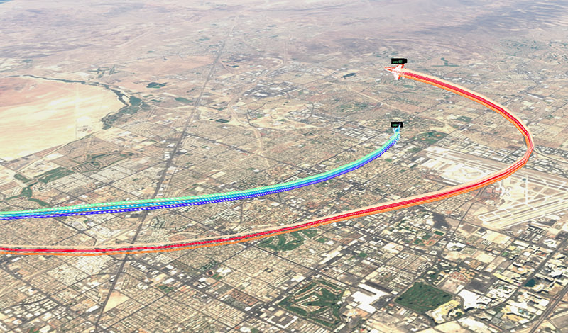
Figure 1: Rendering of the simulation environment

The observation space for each agent includes information about ownship aircraft (fuel load, thrust, control surface deflection, health), aerodynamics (alpha and beta angles), position (local plane coordinates, velocity, and acceleration), and attitude (Euler angles, rates, and accelerations). The agent also gets the position (local plane coordinates and velocity), and attitude (Euler angles and rates) information of its opponent as well as its opponents health. All state information from the environment is provided without modeled sensor noise.

Actions are input 50 times per simulation second. The agent’s actions are continuous and map to the inputs of the F-16’s flight control system (aileron, elevator, rudder, and throttle). The reward given by the environment is based on the agent’s position with respect to its adversary, and its goal is to position the adversary within its Weapons Engagement Zone (WEZ).

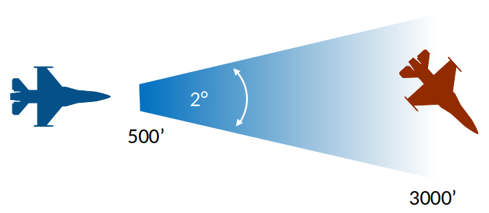
Figure 2: Weapon Engagement Zone (WEZ)

The WEZ is defined as the locus of points that lie within a spherical cone of 2 degree aperture, which extends out of the nose of the plane, that are also 500-3000 ft away (Figure 2). Though the agent isn’t truly taking shots on its opponent, throughout this paper we will call attaining this geometry getting a “gun snap”.

The damage per second to the adversary in the WEZ is given by

$$d_{wez}=\left\{\begin{array}[]{ll}0&r>3000ft\\ \frac{3000-r}{2500}&500ft\leq r\leq 3000ft\\ 0&r<500ft\\ \end{array}\right.$$

where $d_{wez}$ is the damage incurred by being in the WEZ and $r$ is the distance between the aircraft.

The reward given to the agent by the environment is calculated as the area under the opponent’s damage over time curve,

$$r_{t}=\left\{\begin{array}[]{ll}\mathds{E}_{t^{\prime}\in[0,T]}[d_{opp}(t^{\prime})]&d_{self}<1\\ 0&otherwise\\ \end{array}\right.$$

where $r_{t}$ is the reward at time step $t$, $d_{self}$ is the damage to the agent, $d_{opp}$ is the damage to the opponent (Figure 3), and $T=300$, the maximum duration of an engagement.

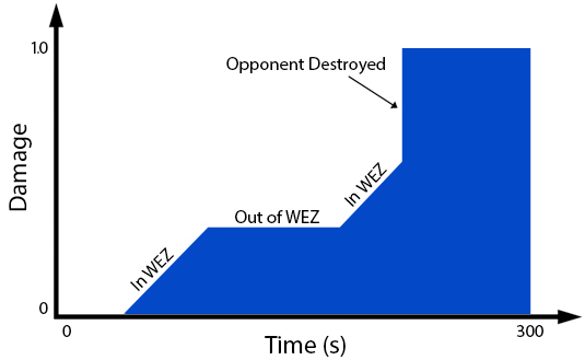
Figure 3: Example of damage calculated over the course of an episode

The engagement starts with both aircraft having full health (health = 1.0) and ends when one or both of the aircraft reach zero health or once the duration of the simulation reaches 300 seconds. An agent ‘wins‘ when its opponent‘s health reaches zero. This can happen when either the opponent dips below the minimum altitude (hard deck) of 1000 ft. or when the opponent incurs sufficient damage through gun snaps. The fight ends in a draw if the engagement times out.

V Agent Architecture

Our agent, PHANG-MAN (Policy Hierarchy for Adaptive Novel Generation of MANeuvers), is composed of a 2-layer hierarchy of policies. On the low level, there is an array of policies that have been trained to excel in a particular region of the state space. At the high level, a single policy selects which low-level policy to activate given the current context of the engagement. Our architecture is shown in Figure 4.

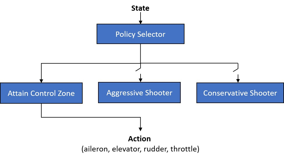
Figure 4: High-level architecture of PHANG-MAN agent

V-A Low Level Policies

All low-level policies are trained with the Soft Actor-Critic (SAC) algorithm [49]. Since SAC is an off-policy RL algorithm in which the actor aims to maximize the expected reward while also maximizing entropy, exploration is maximized alongside performance. Each low-level policy ingests the same state values and has an identical three-layer multilayer perceptron (MLP) architecture. The low-level policies are evaluated and new actions input to the environment at the maximum simulation frequency, 50 Hz. What distinguishes the low-level policies are the range of initial conditions used in training and their respective reward functions. The reward function of each low-level policy is the sum of a variety of independent components, each designed to encourage a specific behavior. A description of the reward function components is given below:

• $R_{\text{$relative$ $position$}}$ rewards the agent for positioning itself behind the opponent with its nose pointing at the opponent. It also penalizes the agent when the opposite situation occurs.

• $R_{\text{$track$ $\theta$}}$ penalizes the agent for having a non-zero track angle (angle between ownship aircraft nose and the center of the opponent aircraft), regardless of its position relative to the opponent.

• $R_{closure}$ rewards the agent for getting closer to the opponent when pursuing and penalizes it for getting closer when being pursued.

• $R_{gunsnap(blue)}$ is a reward given when the agent achieves a minimum track angle and is within a particular range of distances, similar to WEZ damage in the environment.

• $R_{gunsnap(red)}$ is a penalty given when the opponent achieves a minimum track angle and is within a particular range of distances, similar to WEZ damage in the environment.

• $R_{deck}$ penalizes the agent for flying below a minimum altitude threshold.

• $R_{\text{$too$ $close$}}$ penalizes the agent for violating a minimum distance threshold within a range of adverse angles (angle between the opponent’s tail and the center of the ownship aircraft) and is meant to discourage overshooting when pursuing.

An overview of each of the three low-level polices follows:

Control Zone (CZ): The CZ policy will try to attain a pursuit position behind the opponent and occupy a region of the state space that makes it virtually impossible for the opponent to escape, which is also called the “control zone”. The CZ policy was trained with the widest range of initial conditions of any of the low-level policies. The initial conditions were composed of uniformly random positions, Euler angles, and body-frame velocities. Domain knowledge from retired fighter pilots was leveraged to design the CZ policy’s multi-dimentional reward function. The function is dependent on track angle, adverse angle, distance to opponent, height above the hard deck, and closure rate. The CZ reward function is given by $R_{total}=R_{\text{$relative$ $position$}}+R_{closure}+R_{gunsnap(blue)}+R_{gunsnap(red)}+R_{deck}+R_{\text{$too$ $close$}}$. Select surfaces of the CZ policy’s reward function are shown in Figure 5.

Figure 5: $R_{\text{$relative$ $position$}}$, $R_{closure}$, and $R_{gunsnap(blue)}$ components of the CZ policy’s reward function

Aggressive shooter (AS): Unlike the CZ policy, the AS policy is encouraged to take aggressive shots from the side and head on. Gun snap rewards are greater in magnitude at closer distances like the WEZ damage function of the environment. As a result, the AS policy often takes shots that will yield the most damage but leave it susceptible to counter maneuvers. On defense, the AS policy avoids gun snaps from close range more than those from farther away, making it a relatively less aggressive evader. The AS policy was trained with initial conditions that place either the opponent or ownship aircraft within the WEZ, maximizing the time spent learning effective offensive and defensive gun snap maneuvers. The AS reward function is given by $R_{total}=R_{\text{$track$ $\theta$}}+R_{gunsnap(blue)}+R_{gunsnap(red)}+R_{deck}$. Select surfaces of the AS policy’s reward function are shown in Figure 6 (top).

Conservative shooter (CS): The CS policy leveraged the same initial conditions during training and has a similar reward function as the AS policy. The notable difference is the plateau region of the gun snap components in the CS reward function. As a result, the CS policy learned to value gun snaps from near and far equally, resulting in behavior that effectively maintains an offensive scoring position, even though the magnitude of the points scored may be low. On the defensive end, the CS policy avoids gun snaps equally from all distances, making it equally sensitive to all damage and a relatively aggressive evader. The CS reward function is given by $R_{total}=R_{\text{$track$ $\theta$}}+R_{gunsnap(blue)}+R_{gunsnap(red)}+R_{deck}$. The $R_{gunsnap(blue)}$ component of the CS policy’s reward function is shown in Figure 6 (bottom).

Figure 6: $R_{gunsnap(blue)}$ and $R_{gunsnap(red)}$ components of the AS policy’s reward function (top) and $R_{gunsnap(blue)}$ component of the CS policy’s reward function (bottom)

V-B Policy Selector

At the top level of our hierarchy, the policy-selector network identifies the best low-level policy given the current context of the engagement. Our approach is similar to options learning [41], however we do not estimate the terminal conditions directly. Instead, a new selection is made periodically at a frequency of 10 Hz. Unlike the option-critic architecture [50], the selectable policies are trained separately and their parameters are frozen. This enables policy selector training without the complications associated with non-stationary policies [45]. This simplifies the learning problem and permits training and re-use of agents in a modular fashion.

Figure 7: Illustration of agent selection during a single episode. Policy selector (PS) with a team of 3 agents: CZ, CS, and AS. Opponents: CS (top) and CZ (bottom)

The policy selector is implemented using the same SAC algorithm. Although a SAC implementation for discrete actions is viable for choosing low-level policies [51], the continuous version of SAC combined with argmax demonstrated better performance.

The reward function used to train the policy selector closely resembles the WEZ damage function of the environment, which is sparse. To facilitate learning, we also include a reward that is proportional to track angle at every step.

In Figure 7, we show an example of how different agents are dynamically selected depending on the current state. We plot the track angle as a representation of what is happening in this episode. In the match against the CS policy (top), the policy selector agent exploits the initial positional advantage (smaller track angle), closes the distance while reducing the track angle, it overshoots once (step 500) but gets persistent gun snaps (steps 1100 to 1300) and ends the episode with a win.

During policy selector training, in each episode the percent utilization of each low-level policy is computed. When plotted over training episodes, it is observed that the selector learns unique and effective strategies for each opponent. Figure 8 shows how the normalized utilization of selected low-level policies significantly differs when playing against an an intelligent agent such as itself (top) and an agent with random movements, Randy (bottom).

Figure 8: Normalized utilization of low-level policies vs. PHANG-MAN (self-play) and Randy (random maneuver agent)

We observed that the performance of the policy selector against any individual opponent was at least as good as that of the highest performing low-level policy against the same opponent. Additionally, across several opponents, the performance of the policy selector was significantly greater than that of any individual low-level policy, indicating it was able to effectively leverage the strengths of the low-level policies and generate unique complementary strategies.

Hyperparameters for the low-level policies and policy selector are given in Table 1.

TABLE I: List of common hyper-parameters used in the SAC training.

Parameter	Value
Optimizer	Adam
Replay buffer size	5.0e6
Number of hidden layers	1
Number of hidden neurons	7168 (Policy Selector)
	12288 (CZ, AS, CS)
Batch size	256
Learning rate	2.0e-4
Discount factor $\gamma$	0.99
Soft $\tau$	1.0e-3
Entropy target $\tau$	-3 (Policy Selector)
	-4 (CZ, AS, CS)
Activation function	ReLU
Target update interval	1

VI PHANG-MAN at the ADT Final Event

The ADT final event was completed over 3 days of competition. On Day 1, competitors faced agents developed by JHU-APL in collaboration with DARPA. Day 2 involved a Round Robin tournament, in which each team played against all others in a best of 20 match. On Day 3, the top 4 teams at the end of day 2 played in a single elimination championship tournament.

These teams also had the opportunity to play against a graduate of the USAF F-16 Weapons Instructor Course in a best of 5 match.

Our agent finished the initial 2 days of the competition in $2^{nd}$ place, qualifying for the championship tournament. On Day 3, PHANG-MAN won its semi-final round and in the finals was defeated by Heron Systems’ agent, finishing the competition in $2^{nd}$ place overall. The tournament bracket and results are shown in Figure 9. The semi-finals and finals can be viewed online.

In the championship round, we faced a very aggressive, highly accurate, and impressive adversary from Heron Systems. In most cases, PHANG-MAN did not survive the initial exchange of nose-to-nose gun snaps and matches would end with Heron emerging victorious but having very little health remaining. Although we scored 7% more total shots against Heron’s agent, our average shot was from farther away and thus our average damage was lower. Our agent would disengage its offense inside of 800 ft. in favor of better positioning for the next exchange, while Heron’s agent would continue to aggressively pursue head on. As a result of this aggression, when surviving the initial exchange PHANG-MAN was able to attain a commanding offensive position.

We suspect that this bias toward future positioning over immediate scoring is the result of a strategy we used during training in which we artificially inflated the health of the agents by a factor of 10. Additionally, by not providing a reward that was proportional to the opponents remaining health or a reward for fully depleting our opponent’s health, we may have inadvertently allowed our agent to learn to give away near victories.

Overall, PHANG-MAN demonstrated strategic use of aggressive and conservative tactics. We believe it has the potential to be a trustworthy co-pilot or wingman that can effectively execute real-world tactics in which self-preservation is paramount.

For the matches between the top competitors and the human Air Force pilot, a high-fidelity VR enabled cockpit was provided by the DARPA and JHU-APL team (Figure 10). This allowed the human pilot to visually track the opponent AI as he typically would in a real engagement. A dashboard was displayed for the pilot providing a simplified view of pertinent information (e.g track angle, relative distance to opponent, altitude, fuel, etc). As an additional visual assist, an icon pointing out the opponent direction to the pilot, when outside his vision was provided along with a red flashing overlay of the entire pilot’s view when he received a gun snap.

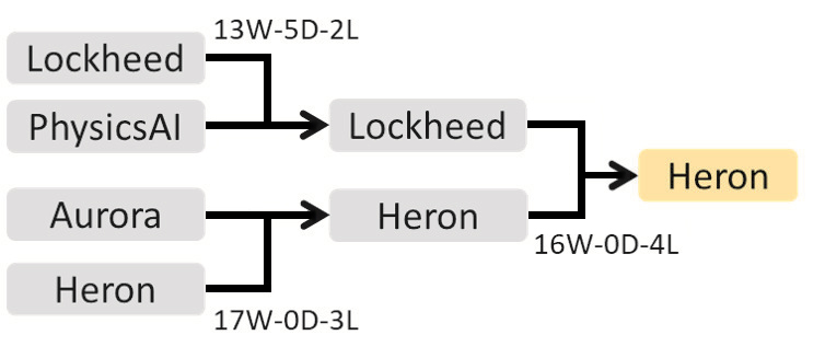
Figure 9: Day 3 tournament results

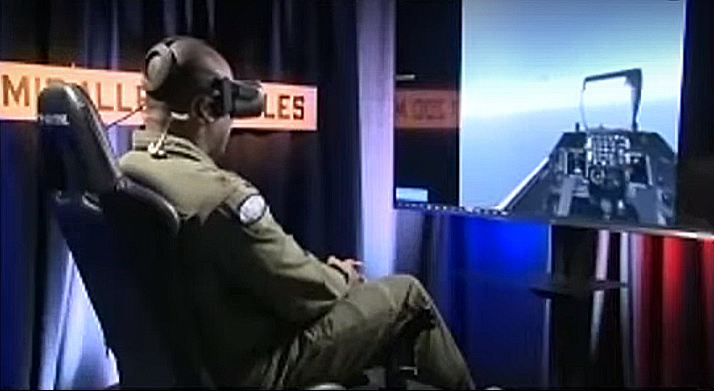
Figure 10: VR enabled cockpit for human vs. AI matchups

PHANG-MAN was one of four agents to emerge victorious (5W - 0L) in its five-game match with the USAF Weapons Instructor pilot. The match-ups were characterized by PHANG-MAN taking aggressive shots from head on and the side, while also capitalizing on any mistakes that the human pilot made that gave up their control zone.

VII Future Work

The quick paced, one-year timeline of ADT provided many new avenues of future research in this problem space. To this end Lockheed Martin is making significant investments to further research and develop this work.

Alongside deeper algorithmic research specific to the air-to-air domain we are adapting our current efforts with the goal of full-scale deployment. Enhancing the simulation environment is the first step in this direction: modification and additions to the observation space (incorporating domain randomization techniques [52], imperfect information, partial/estimated knowledge, etc.) and incorporating different platform aerodynamics models (quad-copter, small fixed-wing unmanned aerial vehicles, F-22, etc.). This will allow for smoother transition as we deploy on sub-scale and eventually full-scale aircraft.

VIII Conclusion

The AlphaDogfight Trials sought to challenge competitors to develop high performing AI agents that can excel in air-to-air combat. We developed a hierarchical agent that succeeded in competition, ranking $2^{nd}$ place overall and defeating a graduate of the US Air Force Weapons School’s F-16 Weapons Instructor Course. LM intends to continue investing in this research and fully explore the potential of these algorithms and their path to deployment.

References

- [1] R. Isaacs, Games of Pursuit,” RAND Corporation, Santa Monica. RAND Corporation, 1951.
- [2] G. H. Burgin and L. Sidor, “Rule-based air combat simulation,” Titan Systems Inc La Jolla CA, Tech. Rep., 1988.
- [3] J. S. McGrew, J. P. How, B. Williams, and N. Roy, “Air-combat strategy using approximate dynamic programming,” Journal of guidance, control, and dynamics, vol. 33, no. 5, pp. 1641–1654, 2010.
- [4] E. Y. Rodin and S. M. Amin, “Maneuver prediction in air combat via artificial neural networks,” Computers & mathematics with applications, vol. 24, no. 3, pp. 95–112, 1992.
- [5] K. Virtanen, J. Karelahti, and T. Raivio, “Modeling air combat by a moving horizon influence diagram game,” Journal of guidance, control, and dynamics, vol. 29, no. 5, pp. 1080–1091, 2006.
- [6] F. Austin, G. Carbone, M. Falco, H. Hinz, and M. Lewis, “Game theory for automated maneuvering during air-to-air combat,” Journal of Guidance, Control, and Dynamics, vol. 13, no. 6, pp. 1143–1149, 1990.
- [7] J. McManus and K. Goodrich, “Application of artificial intelligence (ai) programming techniques to tactical guidance for fighter aircraft,” in Guidance, Navigation and Control Conference, 1989, p. 3525.
- [8] N. Ernest, D. Carroll, C. Schumacher, M. Clark, K. Cohen, and G. Lee, “Genetic fuzzy based artificial intelligence for unmanned combat aerial vehicle control in simulated air combat missions,” Journal of Defense Management, vol. 6, no. 1, pp. 2167–0374, 2016.
- [9] L. A. Zhang, J. Xu, D. Gold, J. Hagen, A. K. Kochhar, A. J. Lohn, and O. A. Osoba, Air Dominance Through Machine Learning: A Preliminary Exploration of Artificial Intelligence: Assisted Mission Planning. Santa Monica, CA: RAND Corporation, 2020.
- [10] Y. Chen, J. Zhang, Q. Yang, Y. Zhou, G. Shi, and Y. Wu, “Design and verification of uav maneuver decision simulation system based on deep q-learning network,” in 2020 16th International Conference on Control, Automation, Robotics and Vision (ICARCV). IEEE, 2020, pp. 817–823.
- [11] J. Xu, Q. Guo, L. Xiao, Z. Li, and G. Zhang, “Autonomous decision-making method for combat mission of uav based on deep reinforcement learning,” in 2019 IEEE 4th Advanced Information Technology, Electronic and Automation Control Conference (IAEAC), vol. 1. IEEE, 2019, pp. 538–544.
- [12] Q. Yang, J. Zhang, G. Shi, J. Hu, and Y. Wu, “Maneuver decision of uav in short-range air combat based on deep reinforcement learning,” IEEE Access, vol. 8, pp. 363–378, 2019.
- [13] W. Kong, D. Zhou, Z. Yang, Y. Zhao, and K. Zhang, “Uav autonomous aerial combat maneuver strategy generation with observation error based on state-adversarial deep deterministic policy gradient and inverse reinforcement learning,” Electronics, vol. 9, no. 7, p. 1121, 2020.
- [14] Z. Wang, H. Li, H. Wu, and Z. Wu, “Improving maneuver strategy in air combat by alternate freeze games with a deep reinforcement learning algorithm,” Mathematical Problems in Engineering, vol. 2020, 2020.
- [15] T. Vogeltanz, “A survey of free software for the design, analysis, modelling, and simulation of an unmanned aerial vehicle,” Archives of Computational Methods in Engineering, vol. 23, pp. 449–514, 2016.
- [16] X. Chen, Y. Chen, and J. Chase, Mobile robots-state of the art in land, sea, air, and collaborative missions, 2009.
- [17] S. J. Russell and P. Norvig, Artificial Intelligence: A Modern Approach (2nd Edition), 3rd ed. Prentice Hall, December 2009.
- [18] R. S. Sutton and A. G. Barto, Reinforcement Learning: An Introduction. Cambridge, MA, USA: A Bradford Book, 2018.
- [19] T. M. Mitchell, Machine Learning. New York: McGraw-Hill, 1997.
- [20] Z.-W. Hong, T.-Y. Shann, S.-Y. Su, Y.-H. Chang, T.-J. Fu, and C.-Y. Lee, “Diversity-driven exploration strategy for deep reinforcement learning,” in Advances in Neural Information Processing Systems, S. Bengio, H. Wallach, H. Larochelle, K. Grauman, N. Cesa-Bianchi, and R. Garnett, Eds., vol. 31. Curran Associates, Inc., 2018.
- [21] M. L. Puterman, Markov decision processes: discrete stochastic dynamic programming. John Wiley & Sons, 1994.
- [22] R. S. Sutton, “Learning to predict by the methods of temporal differences,” Mach. Learn., vol. 3, no. 1, p. 9–44, 1988. [Online]. Available: https://doi.org/10.1023/A:1022633531479
- [23] P. Thomas, “Bias in natural actor-critic algorithms,” in Proceedings of the 31st International Conference on Machine Learning, ser. Proceedings of Machine Learning Research, E. P. Xing and T. Jebara, Eds., vol. 32, no. 1. Bejing, China: PMLR, 22–24 Jun 2014, pp. 441–448.
- [24] J. Schulman, P. Abbeel, and X. Chen, “Equivalence between policy gradients and soft q-learning,” CoRR, vol. abs/1704.06440, 2017. [Online]. Available: http://arxiv.org/abs/1704.06440
- [25] T. Haarnoja, H. Tang, P. Abbeel, and S. Levine, “Reinforcement learning with deep energy-based policies,” in Proceedings of the 34th International Conference on Machine Learning, ser. Proceedings of Machine Learning Research, D. Precup and Y. W. Teh, Eds., vol. 70. International Convention Centre, Sydney, Australia: PMLR, 06–11 Aug 2017, pp. 1352–1361.
- [26] T. Haarnoja, A. Zhou, P. Abbeel, and S. Levine, “Soft actor-critic: Off-policy maximum entropy deep reinforcement learning with a stochastic actor,” in Proceedings of the 35th International Conference on Machine Learning, ser. Proceedings of Machine Learning Research, J. Dy and A. Krause, Eds., vol. 80. Stockholmsmässan, Stockholm Sweden: PMLR, 10–15 Jul 2018, pp. 1861–1870. [Online]. Available: http://proceedings.mlr.press/v80/haarnoja18b.html
- [27] T. Haarnoja, A. Zhou, K. Hartikainen, G. Tucker, S. Ha, J. Tan, V. Kumar, H. Zhu, A. Gupta, P. Abbeel, and S. Levine, “Soft actor-critic algorithms and applications,” CoRR, vol. abs/1812.05905, 2018. [Online]. Available: http://arxiv.org/abs/1812.05905
- [28] B. D. Ziebart, “Modeling purposeful adaptive behavior with the principle of maximum causal entropy,” Ph.D. dissertation, Machine Learning Dpt., Carnegie Mellon University, Pittsburgh, PA, 2010.
- [29] C. J. C. H. Watkins and P. Dayan, “Technical note: q -learning,” Mach. Learn., vol. 8, no. 3–4, p. 279–292, 1992. [Online]. Available: https://doi.org/10.1007/BF00992698
- [30] V. Mnih, K. Kavukcuoglu, D. Silver, A. A. Rusu, J. Veness, M. G. Bellemare, A. Graves, M. Riedmiller, A. K. Fidjeland, G. Ostrovski, S. Petersen, C. Beattie, A. Sadik, I. Antonoglou, H. King, D. Kumaran, D. Wierstra, S. Legg, and D. Hassabis, “Human-level control through deep reinforcement learning,” Nature, vol. 518, pp. 529–533, 2015. [Online]. Available: http://dx.doi.org/10.1038/nature14236
- [31] R. J. Williams, “Simple statistical gradient-following algorithms for connectionist reinforcement learning,” Mach. Learn., vol. 8, no. 3–4, p. 229–256, 1992.
- [32] D. Silver, G. Lever, N. Heess, T. Degris, D. Wierstra, and M. Riedmiller, “Deterministic policy gradient algorithms,” in Proceedings of the 31st International Conference on Machine Learning, ser. Proceedings of Machine Learning Research, E. P. Xing and T. Jebara, Eds., vol. 32, no. 1. Bejing, China: PMLR, 22–24 Jun 2014, pp. 387–395.
- [33] J. Schulman, S. Levine, P. Abbeel, M. Jordan, and P. Moritz, “Trust region policy optimization,” in Proceedings of the 32nd International Conference on Machine Learning, ser. Proceedings of Machine Learning Research, F. Bach and D. Blei, Eds., vol. 37. Lille, France: PMLR, 07–09 Jul 2015, pp. 1889–1897.
- [34] J. Schulman, F. Wolski, P. Dhariwal, A. Radford, and O. Klimov, “Proximal policy optimization algorithms,” CoRR, vol. abs/1707.06347, 2017. [Online]. Available: http://arxiv.org/abs/1707.06347
- [35] T. P. Lillicrap, J. J. Hunt, A. Pritzel, N. Heess, T. Erez, Y. Tassa, D. Silver, and D. Wierstra, “Continuous control with deep reinforcement learning,” in 4th International Conference on Learning Representations, (ICLR 2016), Y. Bengio and Y. LeCun, Eds., 2016.
- [36] J. Schmidhuber, “Learning to generate subgoals for action sequences,” in IJCNN-91-Seattle International Joint Conference on Neural Networks, vol. ii, 1991, pp. 453 vol.2–.
- [37] R. S. Sutton, D. Precup, and S. Singh, “Between mdps and semi-mdps: A framework for temporal abstraction in reinforcement learning,” Artif. Intell., vol. 112, no. 1–2, p. 181–211, 1999.
- [38] P. Dayan and G. E. Hinton, “Feudal reinforcement learning,” in Advances in Neural Information Processing Systems, S. Hanson, J. Cowan, and C. Giles, Eds., vol. 5. Morgan-Kaufmann, 1993.
- [39] A. G. Barto and S. Mahadevan, “Recent advances in hierarchical reinforcement learning,” Discrete Event Dynamic Systems, vol. 13, no. 1–2, p. 41–77, 2003.
- [40] M. M. Botvinick, “Hierarchical reinforcement learning and decision making,” Current Opinion in Neurobiology, vol. 22, no. 6, pp. 956–962, 2012, decision making.
- [41] G. Comanici and D. Precup, “Optimal policy switching algorithms for reinforcement learning,” in Proceedings of the 9th International Conference on Autonomous Agents and Multiagent Systems (AAMAS 2010), 2010, pp. 709–714.
- [42] T. Schaul, D. Horgan, K. Gregor, and D. Silver, “Universal value function approximators,” in Proceedings of the 32nd International Conference on Machine Learning, ser. Proceedings of Machine Learning Research, F. Bach and D. Blei, Eds., vol. 37. Lille, France: PMLR, 07–09 Jul 2015, pp. 1312–1320.
- [43] P.-L. Bacon, J. Harb, and D. Precup, “The option-critic architecture,” in Proceedings of the Thirty-First AAAI Conference on Artificial Intelligence, ser. AAAI’17. AAAI Press, 2017, p. 1726–1734.
- [44] A. S. Vezhnevets, S. Osindero, T. Schaul, N. Heess, M. Jaderberg, D. Silver, and K. Kavukcuoglu, “Feudal networks for hierarchical reinforcement learning,” in Proceedings of the 34th International Conference on Machine Learning - Volume 70, ser. ICML’17. JMLR.org, 2017, p. 3540–3549.
- [45] O. Nachum, S. Gu, H. Lee, and S. Levine, “Data-efficient hierarchical reinforcement learning,” Advances in Neural Information Processing Systems, pp. 3303–3313, 2018.
- [46] Y. Flet-Berliac, “The promise of hierarchical reinforcement learning,” The Gradient, 2019.
- [47] K. Frans, J. Ho, X. Chen, P. Abbeel, and J. Schulman, “Meta learning shared hierarchies,” in 6th International Conference on Learning Representations, (ICLR 2018). OpenReview.net, 2018. [Online]. Available: https://openreview.net/forum?id=SyX0IeWAW
- [48] J. Berndt, “Jsbsim: An open source flight dynamics model in c++,” in Modeling and Simulation Technologies Conference and Exhibit. American Institute of Aeronautics and Astronautics, 2004.
- [49] T. Haarnoja, A. Zhou, P. Abbeel, and S. Levine, “Soft actor-critic: Off-policy maximum entropy deep reinforcement learning with a stochastic actor,” in Proceedings of the 35th International Conference on Machine Learning. PMLR, 2018, pp. 1861–1870.
- [50] P. Bacon, J. Harb, and D. Precup, “The option-critic architecture,” in Proceedings of the Thirty-First AAAI Conference on Artificial Intelligence (AAAI’17). Palo Alto, California: AAAI Press, 2017, pp. 1726–1734.
- [51] P. Christodoulou, “Soft actor-critic for discrete action settings,” 2019, arXiv preprint arXiv:1910.07207.
- [52] J. Tobin, R. Fong, A. Ray, J. Schneider, W. Zaremba, and P. Abbeel, “Domain randomization for transferring deep neural networks from simulation to the real world,” in 2017 IEEE/RSJ international conference on intelligent robots and systems (IROS). IEEE, 2017, pp. 23–30.
- [53] J. Ide, P. Shenoy, A. Yu, and C. Li, “Bayesian prediction and evaluation in the anterior cingulate cortex,” The Journal of Neuroscience : the Official Journal of the Society for Neuroscience, vol. 35, pp. 2039–2047, 2013.