Tempered positive Linnik processes and their representations

Abstract

We study several classes of processes associated with the tempered positive Linnik (TPL) distribution, in both the purely absolutely-continuous and mixed law regimes. We explore four main ramifications. Firstly, we analyze several subordinated representations of TPL Lévy processes; in particular we establish a stochastic self-similarity property of positive Linnik (PL) Lévy processes, connecting TPL processes with negative binomial subordination. Secondly, in finite activity regimes we show that the explicit compound Poisson representations gives rise to innovations following novel Mittag-Leffler type laws. Thirdly, we characterize two inhomogeneous TPL processes, namely the Ornstein-Uhlenbeck (OU) Lévy-driven processes with stationary distribution and the additive process generated by a TPL law. Finally, we propose a multivariate TPL Lévy process based on a negative binomial mixing methodology of independent interest. Some potential applications of the considered processes are also outlined in the contexts of statistical anti-fraud and financial modelling.

Keywords: Tempered positive Linnik processes, subordinated Lévy processes, stochastic self-similarity, Ornstein-Uhlenbeck processes, additive processes, multivariate Lévy processes, Mittag-Leffler distributions

MSC 2010 classification:

1 Introduction

In recent years, a large body of literature has been devoted to the tempering of heavy-tailed laws – in particular, stable laws – which prove to be extremely useful in applications to finance and physics (for a recent introduction to the topic, see the monograph by Grabchak, 2016). Indeed, even if heavy-tailed distributions are well-motivated models in a probabilistic setting, extremely bold tails are not realistic for most real-world applications. This drawback has led to the introduction of models which are morphologically similar to the original distributions even if they display lighter tails. The initial case for adopting models that are similar to a stable distribution and with lighter tails is introduced in physics by Mantegna and Stanley, (1994) and Koponen, (1995), and subsequently in economics and finance by the seminal papers of Boyarchenko and Levendorskiï, (2000) and Carr et al., (2002). For recent accounts on tempered distributions, see e.g. Fallahgoul and Loeper, (2021) and Grabchak, (2019).

From a static distributional standpoint the tempered (or “tilted”) version $X$ of a random variable (r.v.) $Y$ by a parameter $\theta>0$ is obtained through the Laplace transform

$$L_{X}(s)=\frac{L_{Y}(\theta+s)}{L_{Y}(\theta)}\text{ .}$$ (1.1)

From this expression it is apparent that the original r.v. and its tempered version have distributions which are practically indistinguishable for real applications when $\theta$ is small, even if their tail behaviour is radically different in the sense that the former may have infinite expectation, while the latter has all the moments finite.

This methodology is particularly well-adapted to the case in which $Y$ follows an infinitely-divisible distribution, since in that case $X$ is also infinitely-divisible and expression (1.1) only involves a simple manipulation of characteristic exponents. Furthermore, the Lévy measure $\nu_{X}(dt)$ of $X$ is itself a tilted version of that of $Y$, meaning that $\nu_{X}(dt)=e^{-\theta t}\nu_{Y}(dt)$. The described tempering procedure may therefore be easily embedded in the theory of L’evy processes. The relationship on Lévy measures highlights that a tempered Lévy process is one whose small jumps occurrence is essentially indistinguishable from that of the base process, but whose large jumps are much more rare events. Additionally, tempering retains a natural interpretation in terms of equivalent measure changes in probability spaces. Let a measure $P_{\theta}$ be defined by means of the following martingale density

$$dP_{\theta}=e^{-\theta Y_{t}+\phi_{Y}(\theta)t}dP\text{ ,}$$ (1.2)

where $\phi_{Y}$ is the characteristic (Laplace) exponent of $Y$, which goes under the name of Esscher transform. Under $P_{\theta}$, the Lévy process associated to the infinitely-divisible r.v. $Y$ coincides with that associated to $X$. This result is of great importance in application fields where the analysis of the process dynamics under equivalent transformation of measures is of relevance, e.g. option pricing (see Hubalek and Sgarra, 2006).

In the context of tempering of probability laws, Barabesi et al., 2016a introduce the tempered positive Linnik (TPL) distribution as a tilted version of the positive Linnik (PL) distribution considered in Pakes, (1998) and inspired by the classic paper of Linnik, (1963). The PL law has received increasing interest since it constitutes a generalization of the gamma law and recovers the positive stable (PS) law as a limiting case (for details, see Christoph and Schreiber, 2001). Hence, its tempered version is suitable for modelling real data. In addition, the tempering substantially extends the parameter range of the PL law and accordingly gives rise to two distinct regimes embedding positive absolutely-continuous distributions, as well as mixtures of positive absolutely-continuous distributions and the Dirac mass at zero. The latter regime may be useful for modelling zero-inflated data. Finally, the tempered positive stable (TPS) law (or “Tweedie distribution”), which is central in many recent statistical applications, see e.g. Barabesi et al., 2016b , Fontaine et al., 2020, Khalin and Postnikov, 2020, Ma et al., 2018, can also be recovered as a limiting case of the TPL law. A discrete version of the TPL law is suggested in Barabesi et al., 2018a , while computational issues dealing with the TPL and TPS laws are discussed in Barabesi, (2020) and Barabesi and Pratelli, (2014, 2015, 2019).

Regarding the theoretical findings on the TPL law, Barabesi et al., 2016a obtain closed formulas of the probability density function and the conditional probability density function (under the two regimes, respectively) of the TPL random variable in terms of the Mittag-Leffler function and outline the infinite-divisible and self-decomposable character of the corresponding L’evy measures – as well as their representation as a mixture of TPS laws with a gamma mixing density. Kumar et al., 2019b study the gamma subordinated representation of the tempered Mittag-Leffler subclass of TPL L’evy process, its moment and covariance properties and provide alternative derivations of the associated L’evy densities and supporting equations for the probability density function. Leonenko et al., (2021) explore in detail the large deviation theory for TPL processes. Kumar et al., 2019a instead analyze Linnik processes – not necessarily increasing – and their generalizations.

In this paper, we focus on a number of stochastic processes naturally arising from the TPL distribution and illustrate their representations and properties. First of all we provide a detailed account of the infinite divisibility property and unify and clarify the Lévy-Khinctine structure of a TPL law. We also prove additional properties of TPL laws, such as geometric infinite divisibility. We then study the subordinated structure of the TPL Lévy process, showing that besides the defining characterization as a gamma-subordinated law, such laws enjoy numerous representations in terms of a negative binomial subordination. This is in turn connected to the stochastic self-similarity property – as introduced by Kozubowski et al., (2006) – of the PL subordinator with respect to the negative binomial subordinator. We further make clear the role of the tail parameter $\gamma$ in determining two distinct regimes for the processes associated to the TPL distribution. Whenever $\gamma\in(0,1]$, the TPL law is absolutely continuous and an infinite activity process occurs. In contrast, when $\gamma<0$, the TPL has a mixed absolutely-continuous and point mass expression. We then find that the corresponding Lévy process is a compound Poisson process which we show to feature increments of “logarithmic” Mittag-Leffler type. The absolutely-continuous case instead corresponds to a self-decomposable family distributions to which using classic theory (Barndorff-Nielsen, 1997, Sato, 1991) we are able to associate an Ornstein-Uhlenbeck (OU) Lévy-driven process with TPL stationary distribution and an additive TPL process. We characterize such processes. In particular, the Lévy driving noise of the OU process with TPL stationary distribution is a compound Poisson process with tempered Mittag-Leffler distribution, a probability law which as far as the authors are aware has not been considered before. Finally, we concentrate on the multivariate TPL Lévy process constructed from a TPL Lévy process with independent marginals subordinated to a negative binomial subordinator. Such a construction makes again critical use of the stochastic self-similarity property, and can be easily generalized to different subordinand processes. Furthermore, it encompasses some well-known multivariate distributions of common use in the statistical environment.

The paper is organized as follows. In Section 2 – after reviewing some basic known properties – we discuss the infinite divisibility and the L’evy-Khintchine representation, as well as the self-decomposability and geometric infinite divisibility, of the TPL law. Section 3 is devoted to TPL L’evy subordinators and their various representations. In Section 4, we consider the OU L’evy-driven processes with stationary TPL distribution and the additive process generated by a TPL law. In Section 5, we propose the natural multivariate version of the TPL law, and the connected L’evy process. Finally, in Section 6, applications for statistical anti-fraud are considered.

2 The tempered positive Linnik distribution

If $X$ represents a positive random variable (r.v.) on a probability space $(\Omega,\mathcal{F},P)$, we denote its Laplace transform $L_{X}(s)=\mathrm{E}[e^{-sX}]$, for all values of $s\in\mathbb{C}$ for which such expectation exists.

The PL family of laws PL$(\gamma,\lambda,\delta)$ was introduced by Pakes, (1998), on the basis of the original suggestion of Linnik, (1963). A PL r.v. $V$ is characterized by the Laplace transform

$$L_{V}(s)=\left(\frac{1}{1+\lambda s^{\gamma}}\right)^{\delta},\quad\text{Re}(s)>0,$$ (2.1)

$(\gamma,\lambda,\theta)\in\times(0,1]\times\mathbb{R}_{+}\times\mathbb{R}_{+}$. For details on Linnik-type laws see e.g. Christoph and Schreiber, (2001), or more recently Korolev et al., (2020) and references therein.

Barabesi et al., 2016a propose a new family of distributions which is a tempered version of the PL family. By slightly modifying the parametrization thereby proposed, the TPL r.v. $X$ is defined as a member of the four-parameter family TPL$(\gamma,\lambda,\delta,\theta)$ with Laplace transform given by

$$L_{X}(s)=\left(\frac{1}{1+\text{sgn}(\gamma)\lambda((\theta+s)^{\gamma}-\theta^{\gamma})}\right)^{\delta},\quad\text{Re}(s)>0,$$ (2.2)

with parameter space for $(\gamma,\lambda,\delta,\theta)$ given by

$$S=\{(-\infty,1]\setminus\{0\}\times\mathbb{R}_{+}\times\mathbb{R}_{+}\times\mathbb{R}_{+}\}\cup\{(0,1]\times\mathbb{R}_{+}\times\mathbb{R}_{+}\times\{0\}\}.$$ (2.3)

The terminology is motivated by the fact that the genesis of this distribution for $\gamma\in(0,1)$ is that of tempering PL random variables in a way analogous to the classic tempering of stable laws. If $V$ is PL$(\gamma,\lambda,\delta)$ and $\theta>0$ then

$$L_{X}(s)=\frac{L_{V}(\theta+s)}{L_{V}(\theta)}=\left(\frac{1}{1+\lambda^{\prime}((\theta+s)^{\gamma}-\theta^{\gamma})}\right)^{\delta}$$ (2.4)

with $\lambda^{\prime}=\lambda/(1+\lambda\theta^{\gamma})$. See Subsection 2.2 further on for more on this analogy.

The TPL family encompasses the PL law for $\theta=0$, the Mittag-Leffler law proposed by Pillai, (1990) for $\delta=1$ and $\theta=0$, and the gamma law for $\gamma=1$, or – alternatively – for $\gamma\in(0,1]$ and $\lambda\theta^{\gamma}=1$. Furthermore, a TPS$(\gamma,\lambda,\theta)$ can be obtained as a limit in distribution of a TPL$(\gamma,\delta\lambda,\delta,\theta)$ as $\delta\rightarrow\infty$. In addition from (2.2) we see that the TPL family is closed under convolution. More precisely let $(X_{k})_{k\in\mathbb{N}}$ be a sequence of independent r.v.s with TPL$(\gamma,\lambda,\delta_{k},\theta)$ distribution; then $\sum_{k=1}^{n}X_{k}$ has TPL$\left(\gamma,\lambda,\sum_{k=1}^{n}\delta_{k},\theta\right)$ distribution.

The fact that in (2.2) the parameter $\gamma$ is allowed to be negative has many implications and is one of the central aspects of this paper. To begin with, the two parameters subsets $(-\infty,0)$ and $(0,1]$ for $\gamma$ determine distinct regimes in the Lebesgue decomposition of the law of a TPL variable.

Denote with $E_{a,b}^{c}(z)$, $z\in\mathbb{C}$, the Prabhakar, (1971) three-parameter Mittag-Leffler function

$$E_{a,b}^{c}(z)=\sum_{k=0}^{\infty}\frac{(c)_{k}z^{k}}{k!\Gamma(ak+b)},\qquad\text{Re}(a)>0,\quad\text{Re}(b)>0,\quad c\in\mathbb{C},$$ (2.5)

where $(c)_{k}=c(c+1)\ldots(c+k-1)$ is the Pochhammer symbol. The classic one and two-parameter Mittag-Leffler functions $E_{a}$ and $E_{a,b}$ coincide with $E_{a,1}^{1}$ and $E_{a,b}^{1}$ respectively. In Barabesi et al., 2016a it is shown that for $\gamma\in(0,1)$ a TPL random variable $X$ has probability density function (p.d.f.) $f_{X}$ given by

$$f_{X}(x;\gamma,\lambda,\delta,\theta)=\frac{e^{-\theta x}x^{\gamma\delta-1}}{\lambda^{\delta}}E^{\delta}_{\gamma,\gamma\delta}\left(\frac{\lambda\theta^{\gamma}-1}{\lambda}x^{\gamma}\right)\mathds{1}_{\{x>0\}}.$$ (2.6)

In the case $\theta=0$, forcing $\gamma\in(0,1]$, this collapses to the p.d.f. of a PL law, known since Linnik, (1963). However, the authors observe that when instead $\gamma\in(-\infty,0)$ the distribution is not absolutely continuous. Nevertheless, the conditional p.d.f. on the event $\{X>0\}$ is available. For more details on PL and TPL families of laws see Barabesi et al., 2016a and Barabesi et al., 2016b .

2.1 Infinite divisibility and Lévy-Khintchine representation

A key property of the TPL distribution is its infinite divisibility. We recall that a positive random variable $X$ is said to be infinitely-divisible if for all $n=1,2\ldots$, there exist $n$ i.i.d. random variables $X_{k,n}$, $k=1,\ldots,n,$ such that $X=^{d}X_{1,n}+\ldots+X_{n,n}$. Infinite divisibility of a positive r.v. $X$ is equivalent to require that the logarithm of $L_{X}$ is a Bernstein function (Schilling et al., 2012, Lemma 5.8). This means that there exists a positive measure $\nu$ supported on $\mathbb{R}_{+}$ such that $\int_{0}^{\infty}(1\wedge x)\nu(dx)<\infty$ and constants $a,b>0$ such that

$$\phi_{X}(s):=-\log(L_{X}(s))=a+bs+\int_{(0,\infty)}(1-e^{-st})\nu(dt).$$ (2.7)

Equation (2.7) above is called the Lévy-Khintchine decomposition of $X$ and $(a,b,\nu)$ is referred to as the triplet of Lévy characteristics with Lévy measure $\nu$, and the Bernstein function $\phi_{X}$ as the characteristic (Laplace) exponent (see e.g. Sato, 1999).

If $f$ and $g$ are Bernstein functions then so is $f\circ g$ (Schilling et al., 2012, Corollary 3.8, $iii$). Therefore, if $Y$ and $Z$ are independent positive r.v.s then $\phi_{Z}\circ\phi_{Y}$ is the characteristic exponent of some positive infinitely divisible random variable $X$. Moreover, if $(a,b,\mu)$ and $(\alpha,\beta,\rho)$ are the Lévy characteristics triplets respectively of $Y$ and $Z$ the Lévy triplet of $X$ is given by $(\phi_{Z}(a),b\beta,\eta)$, where for all Borel sets $B$

$$\eta(B)=\int_{(0,\infty)}\mu^{Y}_{t}(B)\rho(dt)+b\mu(B),$$ (2.8)

where $(\mu^{Y}_{t})_{t\geq 0}$ is the convolution semigroup of probability measures associated to $\phi_{Y}$ (Schilling et al., 2012, Theorem 5.27). Equation (2.8) has the statistical interpretation of $X$ being a mixture of $Y$ over the mixing density $Z$, and the dynamic interpretation of a subordination of increasing Lévy processes (Sato, 1999, Chapter 30).

We recall that for $(\lambda,\delta)\in\mathbb{R}^{2}_{+}$ the characteristic exponent $\phi_{Z}$ and Lévy density $u_{Z}$ of a gamma $G(\lambda,\delta)$ r.v. $Z$, whose p.d.f. is given by

$$f_{Z}(x;\lambda,\delta)=\frac{x^{\lambda-1}}{\Gamma(\lambda)\delta^{\lambda}}e^{-x/\delta}\mathds{1}_{\{x>0\}},$$ (2.9)

are respectively

$$\phi_{Z}(s) =\delta\log(1+\lambda s),\qquad\text{Re}(s)>-1/\lambda,$$ (2.10)

$$u_{Z}(x) =\delta\frac{e^{-x/\lambda}}{x}\mathds{1}_{\{x>0\}}.$$ (2.11)

The characteristic exponent and Lévy density of a $\text{TPS}(\gamma,\lambda,\theta)$ r.v. $Y$ for $(\gamma,\lambda,\theta)\in\pi^{\delta}(S)$, where $\pi^{\delta}$ is the projection on the $\delta=0$ subspace of $\mathbb{R}^{4}$, is:

$$\phi_{Y}(s) =\text{sgn}(\gamma)\lambda((\theta+s)^{\gamma}-\theta^{\gamma}),\qquad\text{Re}(s)>0,$$ (2.12)

$$u_{Y}(x) =\frac{|\gamma|\lambda}{\Gamma(1-\gamma)}\frac{e^{-\theta x}}{x^{\gamma+1}}\mathds{1}_{\{x>0\}}$$ (2.13)

and for $\gamma\in(0,1)$, the r.v. $Y$ admits the series representation

$$f_{Y}(x;\gamma,\lambda,\theta)=\frac{e^{-\theta x+\lambda\theta^{\gamma}}}{x}\,\sum_{k=1}^{\infty}\frac{1}{k!\Gamma(-k\gamma)}\,\left(-\frac{x^{\gamma}}{\lambda}\right)^{-k}\mathds{1}_{\{x>0\}},$$ (2.14)

which can be obtained by exponentially tilting with parameter $\theta>0$ the series representation given in Sato, (1999, p.88) of the PS $(\gamma,\lambda)$ law.

The following result has been established in Barabesi et al., 2016a by considering limits of the probability measures as $t$ tends to zero. For $\gamma\in(0,1)$ a proof using (2.8) is offered in Kumar et al., 2019b . In the Proposition below, we summarize these results and extend them to the case $\gamma<0$.

Proposition 2.1.

Let $Y$ and $Z$ be independent r.v.s distributed respectively according to a $\text{{ TPS}}(\gamma,\lambda,\theta)$ and a $G(1,\delta)$ law. Then the r.v. $X$ whose characteristic exponent $\phi_{X}$ is given by

$$\phi_{X}(s)=\phi_{Z}(\phi_{Y}(s))$$ (2.15)

has $\text{{TPL}}(\gamma,\lambda,\delta,\theta)$ distribution. As a consequence any TPL r.v. $X$ is infinitely-divisible with triplet $(0,0,\nu)$, where $\nu$ is an absolutely-continuous measure. Furthermore if

$$(\gamma,\lambda,\delta,\theta)\in\{\gamma<0\}\cup\{0<\gamma<1,\lambda\theta^{\gamma}<1\}\subset S$$ (2.16)

then $\nu$ has density $u_{X}$ given by

$$u_{X}(x)=|\gamma|\delta\frac{e^{-\theta x}}{x}\left(E_{|\gamma|}\left(c_{\gamma,\lambda,\theta}\,x^{|\gamma|}\right)-\mathds{1}_{\{\text{{sgn}}(\gamma)=-1\}}\right)\mathds{1}_{\{x>0\}}$$ (2.17)

with

$$c_{\gamma,\lambda,\theta}:=\left(\frac{\lambda\theta^{\gamma}-\text{{sgn}}(\gamma)}{\lambda}\right)^{\text{{sgn}}(\gamma)}.$$ (2.18)

Proof.

Equation (2.15) is straightforward from (2.2), (2.10) and (2.12), and $X$ is infinitely-divisible because both $Z$ and $Y$ are.

Let us now assume $\gamma\in(0,1)$. We can apply (2.8) with $\mu_{t}^{Y}$ being the absolutely-continuous measures given by the densities $f_{Y}(x;\gamma,t\lambda,\theta)$ from (2.14) and the Lévy triplet $(0,0,\delta\frac{e^{-t}}{t}\mathds{1}_{\{t>0\}}dt)$ characterizing $Z$. Whenever $\lambda\theta^{\gamma}<1$ this gives for $x>0$ a uniformly-integrable series, which we can integrate term by term to get the following Lévy density for $X$

$$u_{X}(x) =\delta\frac{e^{-\theta x}}{x}\sum_{k=1}^{\infty}\frac{1}{k!\Gamma(-k\gamma)}\,\left(-\frac{x^{\gamma}}{\lambda}\right)^{-k}\int_{0}^{\infty}t^{k-1}e^{\left(\lambda\theta^{\gamma}-1\right)t}dt$$

$$=\delta\frac{e^{-\theta x}}{x}\sum_{k=1}^{\infty}\frac{1}{k\Gamma(-k\gamma)}\,\left(\frac{\lambda\theta^{\gamma}-1}{\lambda}x^{\gamma}\right)^{-k}$$

$$=-\gamma\delta\frac{e^{-\theta x}}{x}\sum_{k=1}^{\infty}\frac{1}{\Gamma(1-k\gamma)}\,\left(c_{\gamma,\lambda,\theta}\,x^{\gamma}\right)^{-k}$$

$$=\gamma\delta\frac{e^{-\theta x}}{x}E_{\gamma}\left(c_{\gamma,\lambda,\theta}\,x^{\gamma}\right)$$ (2.19)

after having applied Haubold et al., (2011), Equation (9.2), in the second to last line.

If instead $\gamma<0$ we observe that we can rewrite

$$\phi_{Y}(s)=\lambda\theta^{\gamma}\left(1-\left(\frac{1}{1+s/\theta}\right)^{-\gamma}\right)=\lambda\theta^{\gamma}(1-e^{-\phi_{Z}(s)}),$$ (2.20)

where $Z$ has law $G(-\gamma,1/\theta)$. Therefore $Y$ is in distribution a compound Poisson process with Lévy density $\lambda\theta^{\gamma}f_{Z}$ where $f_{Z}$ is the p.d.f. of $Z$, and the measures $\mu^{Y}_{t}$ are the laws of $Y$ with intensity $\lambda\theta^{\gamma}$ and i.i.d. excursions $Z$. It is well-known (e.g. Sato, 1999) that $\mu^{Y}_{t}$ have the Lebesgue decomposition, for any Borel set $B$:

$$\mu^{Y}_{t}(B) =e^{-\lambda\theta^{\gamma}t}\delta_{0}(B)+\sum_{k=1}^{\infty}\frac{e^{-\lambda\theta^{\gamma}t}}{k!}(\lambda\theta^{\gamma}t)^{k}\int_{B}f^{*k}_{{Z}}(x)dx$$

$$=e^{-\lambda\theta^{\gamma}t}\delta_{0}(B)+\sum_{k=1}^{\infty}\frac{e^{-\lambda\theta^{\gamma}t}}{k!}(t\lambda)^{k}\int_{B}\frac{x^{-\gamma k-1}}{\Gamma(-\gamma k)}e^{-\theta x}dx$$ (2.21)

with the usual convolution notation and where $\delta_{0}$ is the Dirac distribution concentrated in 0. According to (2.8) we have the uniformly integrable series:

$$u_{X}(x) =\delta\frac{e^{-\theta x}}{x}\sum_{k=1}^{\infty}\frac{x^{-\gamma k}}{k!\Gamma(-\gamma k)}\lambda^{k}\int_{0}^{\infty}t^{k-1}e^{-\left(\lambda\theta^{\gamma}+1\right)t}dt$$

$$=\delta\frac{e^{-\theta x}}{x}\sum_{k=1}^{\infty}\frac{1}{k\Gamma(-\gamma k)}\left(\frac{\lambda}{\lambda\theta^{\gamma}+1}x^{-\gamma}\right)^{k}$$

$$=-\gamma\delta\frac{e^{-\theta x}}{x}\left(E_{-\gamma}\left(c_{\gamma,\lambda,\theta}\,x^{-\gamma}\right)-1\right).$$ (2.22)

Combining (2.1) and (2.1) yields (2.17). ∎

The case $\theta=0$ recovers the Lévy measure of the PL distribution as given in e.g. Barndorff-Nielsen, (2000).

Equation (2.17) serves as a starting point for the analysis of the processes based on a TPL a law. Furthermore, it provides the structure of the cumulants of a TPL distribution. The following result is new.

Proposition 2.2.

Under the parameters restrictions and in the notation of Proposition 2.1 and assuming additionally $\theta\neq 0$, for $n\in\mathbb{N}$ let $\kappa^{+}_{n}$ and $\kappa^{-}_{n}$ be the cumulants of the TPL distribution respectively in the regimes $\gamma\in(0,1)$ and $\gamma\in(-\infty,0)$. We have

$$\kappa^{\pm}_{n}=\frac{|\gamma|\delta}{\theta^{n}}g_{n-1}^{\pm}\left(\frac{c_{\gamma,\lambda,\theta}}{\theta^{|\gamma|}}\right)$$ (2.23)

where $g^{\pm}_{n}(x)$ satisfy the recursion

$$g^{\pm}_{n}(x)=x|\gamma|\frac{d}{dx}g^{\pm}_{n-1}(x)+ng^{\pm}_{n-1}(x).$$ (2.24)

with, for $|x|<1$,

$$g^{+}_{0}(x)=\frac{1}{1-x},\qquad g^{-}_{0}(x)=\frac{x}{1-x}.$$ (2.25)

Proof.

By differentiating the characteristic function, the cumulants of a positive infinitely-divisible distribution can be seen to be given by the $n$-th moment integral (modulo adding the linear characteristic when $n=1$) of the Lévy measure. In our case, recalling (2.8), we have when $\gamma\in(0,1)$:

$$\kappa^{+}_{n} =\int_{0}^{\infty}x^{n}u_{X}(x)dx=\gamma\delta\int_{0}^{\infty}e^{-\theta x}\sum_{k=0}^{\infty}\frac{1}{\Gamma(k\gamma+1)}\,c_{\gamma,\lambda,\theta}^{k}x^{\gamma k+n-1}dx$$

$$=\gamma\delta\sum_{k=0}^{\infty}\frac{1}{\Gamma(k\gamma+1)}\,c_{\gamma,\lambda,\theta}^{k}\int_{0}^{\infty}x^{\gamma k+n-1}e^{-\theta x}dx$$

$$=\frac{\gamma\delta}{\theta^{n}}\sum_{k=0}^{\infty}\frac{\Gamma(k\gamma+n)}{\Gamma(k\gamma+1)}\,\left(\frac{c_{\gamma,\lambda,\theta}}{\theta^{\gamma}}\right)^{k}=\frac{\gamma\delta}{\theta^{n}}\sum_{k=0}^{\infty}\left(\frac{c_{\gamma,\lambda,\theta}}{\theta^{\gamma}}\right)^{k}(k\gamma+1)_{n-1}$$ (2.26)

which is a convergent series. The generating function of $g^{+}_{n}(x)=\sum_{k=0}^{\infty}(k\gamma+1)_{n}x^{k}$ of the sequence $a_{k}=(\gamma k+1)_{n}$ when $n$ is fixed can be treated as follows

$$\sum_{k=0}^{\infty}(k\gamma+1)_{n}x^{k} =\sum_{k=0}^{\infty}k\gamma(k\gamma+1)_{n-1}x^{k}+n\sum_{k=0}^{\infty}(k\gamma+1)_{n-1}x^{k}$$

$$=\gamma x\frac{d}{dx}\left(\sum_{k=0}^{\infty}(k\gamma+1)_{n-1}x^{k}\right)+n\sum_{k=0}^{\infty}(k\gamma+1)_{n-1}x^{k}$$ (2.27)

Since $g^{+}_{0}(x)=1/(1-x)$, (2.24) follows in the positive $\gamma$ regime.

If instead $\gamma<0$ we have

$$\kappa^{-}_{n} =\int_{0}^{\infty}x^{n}u(x)dx=-\gamma\delta\int_{0}^{\infty}e^{-\theta x}\sum_{k=1}^{\infty}\frac{1}{\Gamma(-k\gamma+1)}\,c_{\gamma,\lambda,\theta}^{k}x^{-\gamma k+n-1}dx$$

$$=-\gamma\delta\sum_{k=1}^{\infty}\frac{1}{\Gamma(k\gamma+1)}\,c_{\gamma,\lambda,\theta}^{k}\int_{0}^{\infty}x^{-\gamma k+n-1}e^{-\theta x}dx$$

$$=-\frac{\gamma\delta}{\theta^{n}}\sum_{k=1}^{\infty}\frac{\Gamma(-k\gamma+n)}{\Gamma(-k\gamma+1)}\,\left(c_{\gamma,\lambda,\theta}\,\theta^{\gamma}\right)^{k}=\frac{(-\gamma)\delta}{\theta^{n}}\sum_{k=1}^{\infty}\left(c_{\gamma,\lambda,\theta}\,\theta^{\gamma}\right)^{k}(-k\gamma+1)_{n-1}$$ (2.28)

and the series again converges for all the admissible parameters values. Setting $g^{-}_{n}(x)=\sum_{k=1}^{\infty}(-k\gamma+1)_{n}x^{k}$ applying (2.1) and observing $g^{-}_{0}(x)=x/(1-x)$ completes the proof. ∎

From (2.23) we find the mean and variance of a TPL r.v. $X$ to be

$$\mathrm{E}[X]=|\gamma|\delta\lambda\theta^{\gamma-1},\qquad\mathrm{Var}[X]=\frac{\mathrm{E}[X]}{\delta}\left(\frac{1-\gamma}{\theta}+\mathrm{E}[X]\right)$$ (2.29)

which correspond to those calculated in Barabesi et al., 2016a (albeit in a different parametrization).

2.2 Self-decomposability and geometric infinite divisibility

A further property of an infinitely-divisible distribution is self-decomposability. A random variable $X$ is said to be self-decomposable if for all $\alpha\in(0,1)$ there exists a r.v. $X_{\alpha}$ independent from $X$ such that $X=^{d}\alpha X+X_{\alpha}$. A self-decomposable distribution is known to be infinitely divisible, and absolutely continuous with an absolutely continuous Lévy density (Steutel and Van Harn,, 2004). Several stochastic processes can be canonically constructed starting from a self-decomposable law, something that we shall exploit in Section 4 once the self-decomposable nature of a TPL r.v. is established.

Another property stronger than infinite divisibility is geometric infinite divisibility introduced by Klebanov et al., (1985). A random variable $X$ is said to be geometrically infinitely-divisible (g.i.d.) if for any $p\in(0,1)$, there exists a geometric random variable $G_{p}$ with probability mass function (p.m.f.)

$$P(G_{p}=k)=p^{k-1}(1-p),\qquad k=1,2,\ldots,$$ (2.30)

and i.i.d. r.v.s $Z_{n,p}$, $n=1,2,\ldots,$ such that

$$X=^{d}\sum_{n=1}^{G_{p}}Z_{n,p}.$$ (2.31)

For example a Mittag-Leffler random variable is g.i.d., as shown in Lin, (1998) Remark 2. For other properties of the g.i.d. random variables see Klebanov et al., (1985), Kalashnikov, (1997) and Kozubowski and Rachev, (1999).

Proposition 2.3.

A TPL$(\gamma,\lambda,\delta,\theta)$ r.v. with $\gamma\in(0,1]$ is self-decomposable. A TPL$(\gamma,\lambda,1,\theta)$ random variable is g.i.d. for all admissible values of $\gamma$.

Proof.

Regarding self-decomposability, according to Steutel and Van Harn, (2004) Proposition V.2.14, it is sufficient to check the case $\theta=0$, i.e. to show self-decomposability of a PL law. This is well-known (see e.g. Christoph and Schreiber, 2001, Section 1.2).

To show geometric infinite-divisibility observe that as observed by Klebanov et al., (1985), Theorem 2, a distribution is g.i.d. if and only if its characteristic function $\psi_{X}(z)$ is such that $1-1/\psi_{X}(z)$ is a characteristic Fourier exponent $\phi_{R}(-iz)=-\log(L_{R}(-iz))$, $z\in\mathbb{C}$, of an infinitely-divisible r.v. $R$. However, if $X$ has distribution TPL$(\gamma,\lambda,1,\theta)$ we have

$$1-\frac{1}{L_{X}(-iz)}=\text{sgn}(\gamma)\lambda((\theta-iz)^{\gamma}-\theta^{\gamma})$$ (2.32)

which is the Fourier characteristic exponent of a TPS$(\gamma,\lambda,\theta)$ law. ∎

If $\gamma<0$ then a TPL r.v. is not self-decomposable since it is not absolutely continuous. The proposition above together with (2.4) clarifies the interpretation of TPL laws as “geometric” analogues of TPS laws, or their “geometric versions”, in the terminology of Sandhya and Pillai, (1999).

In analogy with stable laws one may wish to investigate the stability condition for $p\in(0,1)$ and some $\alpha>0$

$$X=^{d}p^{1/\alpha}\sum_{n=1}^{G_{p}}Z_{n,p}$$ (2.33)

(see Kalashnikov, 1997) where $X$ has $Z_{1,p}$ distribution. A r.v. satisfying (2.33) is said to be geometrically strictly stable (Klebanov et al., 1985, Definition 2). Applying Lin, (1998) Remark 2 shows that PL$(\gamma,\lambda,1)$ (i.e. Mittag-Leffler) r.v.s satisfy (2.33). However, a TPL$(\gamma,\lambda,1,\theta)$ r.v. with $\theta>0$ does not. Indeed (2.33) is very close to characterizing Linnik distributions, and does in fact characterize symmetric or positive ones (Lin, 1994, Lin, 1998).

3 TPL Lévy subordinators and their representation

Being the set of the TPL distributions an infinitely-divisible class, by the general theory for a given TPL$(\gamma,\lambda,\delta,\theta)$ law on $(\Omega,\mathcal{F},P)$ there exists a unique in law increasing Lévy process (Lévy subordinator) $X=(X_{t})_{t\geq 0}$ supported on some filtered probability space $(\Omega,\mathcal{F},\mathcal{F}_{t},P)$ such that $X_{1}$ has one such prescribed law. Furthermore

$$L_{X_{t}}(s)=\mathrm{E}[e^{-sX_{t}}]=e^{-t\phi_{X}(s)}$$ (3.1)

and therefore the r.v.s $X_{t}$ have TPL$(\gamma,\lambda,t\delta,\theta)$ distribution.

The Laplace exponent of the Lévy subordinator is by definition the Laplace exponent of its unit time marginal. Henceforth, when we refer to a Lévy process using a distribution, we mean the Lévy process having such distribution as unit time margin. The Lévy measure of a process is the Lévy measure of its unit time margin. Unless otherwise stated, when we write equality of processes we mean equality of the finite-dimensional distributions.

The TPL process $X$ enjoys a plethora of different representations. The main one is provided directly by Proposition 2.1 and is given by Lévy subordination. Since the characteristic exponent of $X$ is the composition of the characteristic exponents of a gamma law and a TPS law then for all $t$:

$$L_{X_{t}}(s)=e^{-t\phi_{Z}(\phi_{Y}(s))}$$ (3.2)

and therefore by a familiar conditioning argument

$$X_{t}=^{d}Y_{Z_{t}}.$$ (3.3)

In other words $X$ can be represented as a TPS$(\gamma,\lambda,\theta)$ process $Y=(Y_{t})_{t\geq 0}$ (a tempered stable subordinator) subordinated to an independent $G(1,\delta)$ subordinator $Z=(Z_{t})_{t\geq 0}$. We indicate subordination of a process $Y$ to $Z$ with $X=Y_{Z}$.

Remark 3.1.

Associating differently the scale parameter, a fully equivalent representation in distribution for the TPL process is of the form $X=Y^{\prime}_{Z^{\prime}}$ where $Y^{\prime}$ is a TPS$(\gamma,1,\theta)$ process and $Z^{\prime}$ a $G(\lambda,\delta)$ independent subordinator.

From (2.12) we have that $\int_{0}^{\infty}\nu^{Y}(dx)=\infty$ or $\int_{0}^{\infty}\nu^{Y}(dx)<\infty$ depending on whether $\gamma<0$ or $\gamma\in(0,1]$. In the latter case the process $Y$ is of finite activity, that is, $Y$ is a compound Poisson process (CPP). Furthermore, as already observed:

$$\phi_{Y}(s)=\lambda\theta^{\gamma}(1-e^{-\phi_{Z}(s)})$$ (3.4)

where $Z$ is a $G(-\gamma,1/\theta)$ r.v.. Thus $Y$ is a CPP that can be written explicitly as

$$Y_{t}=\sum_{n=0}^{N_{t}}Z_{n},$$ (3.5)

where $Z_{n}$, $n\geq 0$ are i.i.d. with same distribution as $Z$ and $(N_{t})_{t\geq 0}$ is a Poisson process of rate $\lambda\theta^{\gamma}$ independent of the $Z_{n}$s.

The case $\gamma<0$ is of particular interest for data modelling (see e.g. Barabesi et al., 2016b ). In such a case $Y$ is of finite activity and the representation above holds we shall write $Y_{-}$, and $Y_{+}$ when instead $\gamma\in(0,1]$. Correspondingly we define $X_{-}$ and $X_{+}$. Although these Lévy process have different path properties representation (3.3) holds in both cases.

3.1 Compound Poisson representation and the logarithmic Mittag-Leffler distribution

Since $Y_{-}$ is a driftless CPP process, then equation (2.8) and Fubini’s Theorem imply that $X_{-}$ must be a CPP too. In the following we explicitly identify its structure.

In applications the following class of functions is of interest

$$p(x;a,b,c,\alpha,\beta)=x^{a-1}E_{\alpha,\beta}(cx^{b}),\qquad x,a,b>0,\;c\in\mathbb{R},\;\text{Re}(\alpha),\text{Re}(\beta)>0,$$ (3.6)

which are often seen to appear in connection with the solution of fractional differential problems. We can express the Laplace transform $L(\cdot;x,s)$, Re$(s)>0$, of (3.6) in terms of the Fox-Wright function (e.g. Wright, 1935) as follows (Mathai and Haubold, 2008, equation 2.2.22):

$$L(p(x;a,b,c,\alpha,\beta);x,s)= \int_{0}^{\infty}e^{-sx}x^{a-1}E_{\alpha,\beta}(cx^{b})dx=\sum_{k=0}^{\infty}\frac{\Gamma(ak+b)}{\Gamma(\alpha k+\beta)}\frac{c^{k}}{s^{ak+b}}$$

$$= \frac{1}{s^{b}}\phantom{c}_{2}\Psi_{1}\left[\begin{array}[]{cc}(1,1)&(b,a)\\ (\beta,\alpha)&\end{array};\frac{c}{s^{a}}\right],\qquad|c|<|s^{a}|.$$ (3.9)

This latter expression is not always the transform of a probability function. For example in

$$L(p(x;a,b,-1,a,b);x,s)=\frac{s^{a-b}}{s^{a}+1},$$ (3.10)

a function which is pivotal to fractional calculus and its applications (e.g. Haubold et al., 2011), we have that as $s\rightarrow 0$, then $L(p(x;a,b,-1,b,1),x,s)\rightarrow 1$ if and only if $a=b$, in which case the associated distribution is the Mittag-Leffler distribution.

However we can exponentially temper (3.6) by $\theta>0$ obtaining, with slight notation abuse,

$$p(x;a,b,c,\alpha,\beta,\theta)=e^{-\theta x}x^{a-1}E_{\alpha,\beta}(cx^{b}),\qquad x,a,b,\theta>0,\,c\in\mathbb{R},\,\text{Re}(\alpha),\,\text{Re}(\beta)>0,$$ (3.11)

which in turn after applying the shifting rule determines the Laplace transform

$$L(p(x;a,b,c,\alpha,\beta,\theta);x,s)=\frac{1}{(s+\theta)^{b}}\phantom{c}_{2}\Psi_{1}\left[\begin{array}[]{cc}(1,1)&(b,a)\\ (\beta,\alpha)&\end{array};\frac{c}{(s+\theta)^{a}}\right],\qquad|c|<|(s+\theta)^{a}|.$$ (3.14)

As $s\rightarrow 0$ the limit of the expression of the above is always finite, so after appropriate normalization, $p(x;a,b,c,\alpha,\beta,\theta)$ determines a probability distribution. In particular if we let $a=b=\alpha$, $\beta=a+1$, $|c|<\theta^{a}$ we have:

$$L(p(x;a,a,c,a,a+1,\theta),x,s) =\frac{1}{ac}\sum_{k=0}^{\infty}\frac{1}{k+1}\left(\frac{c}{(\theta+s)^{a}}\right)^{k+1}$$

$$=-\frac{1}{ac}{\log\left(1-c(s+\theta)^{-a}\right).}$$ (3.15)

Therefore, defining the normalizing constant

$$n(a,c,\theta)=-\frac{ac}{\log\left(1-c\theta^{-a}\right)},$$ (3.16)

we conclude that $n(a,c,\theta)p(x;a,a,c,a,a+1,\theta)$ is a p.d.f. of known Laplace transform. Calculating this product explicitly we can introduce the following probability distribution.

Definition 3.1.

The logarithmic Mittag-Leffler (LML) distribution is the absolutely-continuous family of distributions LML$(a,c,\theta)$, $a,\theta>0$, $|c|<\theta^{a}$, such that an LML r.v. $W$ has p.d.f.

$$f_{W}(x;a,c,\theta)=-\frac{ac}{\log\left(1-c\theta^{-a}\right)}e^{-\theta x}x^{a-1}E_{a,a+1}(cx^{a})\mathds{1}_{\{x>0\}}$$ (3.17)

and Laplace transform

$$L_{W}(s)=\frac{\log\left(1-c(s+\theta)^{-a}\right)}{\log\left(1-c\theta^{-a}\right)},\qquad\text{{Re}}(s)>0.$$ (3.18)

The terminology is motivated by the similitude of the Laplace transform of this distribution with that of the discrete logarithmic probability law. This distribution is not a generalization of the Mittag-Leffler law as it does not admit it as a particular case, nor does it admit the degenerate case $\theta=0$. Hence it is structurally different from a TPL law. As it turns out, the LML law arises naturally in the CPP structure of $X_{-}$.

Proposition 3.2.

The process $X_{-}$ admits the CPP representation

$$X_{-_{\,t}}=\sum_{n=0}^{N_{t}}J_{n}$$ (3.19)

where $(N_{t})_{t\geq 0}$ is a Poisson process of rate $\delta\log(1+\lambda\theta^{\gamma})$ and $(J_{n})_{n\geq 0}$, is an i.i.d. sequence of random variables having LML$(-\gamma,c_{\gamma,\lambda,\theta},\theta)$ distribution, where $c_{\gamma,\lambda,\theta}$ is given by (2.18).

Proof.

Because of (2.8) $X_{-}$ is driftless, being the gamma subordination of the driftless CPP in (3.5). Using Haubold et al., (2011) Theorem 5.1 in the negative determination of (2.17), we have the equivalent expression for the Lévy density of $X_{-}$:

$$u_{X_{-}}(x)=-\gamma\delta c_{\gamma,\lambda,\theta}e^{-\theta x}x^{-\gamma-1}E_{-\gamma,-\gamma+1}(c_{\gamma,\lambda,\theta}x^{-\gamma})\mathds{1}_{\{x>0\}}.$$ (3.20)

But $c_{\gamma,\lambda,\theta}\theta^{\gamma}<1$ so that from (3.20) and (3.17) we have

$$u_{X_{-}}(x)=\delta\log(1+\lambda\theta^{\gamma})f_{W}(x;-\gamma,c_{\gamma,\lambda,\theta},\theta)\mathds{1}_{\{x>0\}}$$ (3.21)

which proves the proposition. ∎

Another type of tilted Mittag-Leffler distribution following the construction outlined in this section will appear in Section 4.

3.2 Stochastic self-similarity and negative binomial subordination

The TPL processes subordinated structure is extremely rich and and, for reasons which we shall shortly explore, mostly revolves around the negative binomial subordinator. We introduce a lattice-valued version of the Lévy subordinator $B=(B_{t})_{t\geq 0}$ with unit time distribution in the family of laws NB$(\pi,\kappa,\alpha,\mu)$ given by the Laplace transform

$$L_{B}(s)=\left(\frac{\pi}{1-(1-\pi)e^{-\alpha s}}\right)^{\kappa}e^{-\mu s},\qquad\pi\in(0,1),\kappa,\alpha>0,\mu\in\mathbb{R},\text{Re}(s)>0.$$ (3.22)

The above law is a scale-location modification of the negative binomial law, and it thus gives raise to an infinitely-divisible distribution. Taking the logarithm of $L_{B}$ and considering the corresponding characteristic exponent we see that $B$ is such that $B_{t}$ has NB$(\pi,\kappa t,\alpha,\mu)$ distribution and it can be represented as a CPP with drift as follows:

$$B_{t}=\sum_{n=0}^{N_{t}}J_{n}+\mu t$$ (3.23)

with the $J_{n}$ being i.i.d distributed r.v.s with lattice-valued logarithmic probability mass function

$$P(J_{n}=\alpha k)=\frac{(1-\pi)^{k}}{-k\log\pi},\qquad k=1,2,\ldots,$$ (3.24)

and $N=(N_{t})_{t\geq 0}$ is an independent Poisson process of intensity $-\kappa\log\pi$. For these and other properties of the negative binomial subordinator see Kozubowski and Podgórski, (2009).

Negative binomial processes appear naturally in connection to the concept of stochastic self-similarity introduced in Kozubowski et al., (2006), Definition 4.1. Let $X=(X_{t})_{t\geq 0}$ be any stochastic process and assume that there exists a family of processes $T^{c}=\{(T^{c}_{t})_{t\geq 0},c>1\}$ almost surely increasing and diverging as $t\rightarrow\infty$ such that

$$X_{T^{c}_{t}}=^{d}c^{H}X_{t}$$ (3.25)

for some $H>0$. Then $X$ is said to be stochastically self-similar of index $H$ with respect to $T^{c}$.

Stochastic self-similarity is intimately related to geometric infinite-divisibility and in particular to the stability property. Based on this relationship we establish a general invariance property of the PL processes which extends Kozubowski et al., (2006), Proposition 4.2, and which in particular implies that Linnik processes are stochastically self-similar with respect to families of negative binomial processes (see also Barndorff-Nielsen et al., 2001, Example 2.2).

Proposition 3.3.

Let $X=(X_{t})_{t\geq 0}$ be a PL$(\gamma,\lambda,\delta)$ Lévy process, let $H>0$ and let $B^{c}=\{(B^{c}_{t})_{t\geq 0},c>1\}$ be a family of NB$(c^{-H},\kappa,1/\delta,\kappa/\delta)$ subordinators independent of $X$. Then $Y=X_{B^{c}}$ is a PL$(\gamma,\lambda c^{H},\kappa)$ process for all $c>1$. In particular, $X$ is stochastically self-similar for all indices $H>0$ with respect to $B^{c}$.

Proof.

The first claim is equivalent to $\phi_{B^{c}}(\phi_{X}(s))=\phi_{Y}(sc^{H})$ for all Re$(s)>0$ and $c>1$. Composing the exponents and using (3.22)

$$\phi_{B^{c}}(\phi_{X}(s)) =-\kappa\log\left(\frac{c^{-H}e^{-\phi_{X}(s)/\delta}}{1-(1-c^{-H})e^{-\phi_{X}(s)/\delta}}\right)=-\kappa\log\left(\frac{c^{-H}(1+\lambda s^{\gamma})^{-1}}{1-(1-c^{-H})(1+\lambda s^{\gamma})^{-1}}\right)$$

$$=\kappa\log\left(1-c^{H}+c^{H}(1+\lambda s^{\gamma})\right)=\kappa\log\left(1+c^{H}\lambda s^{\gamma}\right)$$ (3.26)

Stochastic self-similarity follows setting $\kappa=\delta$. ∎

Using the subordinated structure of the TPL Lévy process, the distributional invariance part of the proposition above can be extended to $X_{+}$, although stochastic self-similarity does not hold because PL and TPL processes scale differently.

Corollary 3.4.

Let $X$ be a TPL$(\gamma,\lambda,\delta,\theta)$ Lévy process and $B^{\pi}=\{(B^{\pi}_{t})_{t\geq 0},\pi\in(0,1)\}$ be a family of NB$(\pi,\kappa,1/\delta,\kappa/\delta)$ subordinators independent of $X$. Then $X^{\pi}=X_{B^{\pi}}$ is a TPL$(\gamma,\lambda\pi^{-1},\kappa,\theta)$ Lévy process for all $\pi\in(0,1)$.

Proof.

Using Remark 3.1 we recall $X=Y_{Z}$ where $Y$ is a TPS${(\gamma},1,\theta)$ subordinator and $Z$ is a gamma $G(\lambda,\delta)$ process. Applying Proposition 3.3 with $\gamma=H=1$, $c=\pi^{-1}$ we have that $Z^{\pi}:=Z_{B^{\pi}}$ is a $G(\lambda\pi^{-1},\kappa)$ gamma process. Using independence we have the equalities

$$X^{\pi}_{t}=^{d}(Y_{Z})_{B^{\pi}_{t}}=^{d}Y_{Z^{\pi}_{t}}$$ (3.27)

and the conclusion follows using again Remark 3.1 . ∎

Unit scale negative binomial subordinators provide an additional representation for non-degenerate ($\theta>0$) TPL Lévy processes $X_{+}$ and $X_{-}$ as subordinated gamma processes seemingly unrelated to the results above.

Proposition 3.5.

For $\gamma\in(-\infty,0)\cup(0,1)$, $\theta>0$, let $Z$ be a gamma $G(\theta,|\gamma|)$ Lévy process and $B^{\pi}_{+}$ and $B_{-}^{\pi}$ to be two negative binomial processes independent of $Z$ respectively of unit marginals NB$(\pi,\delta,1,\delta)$ and NB$(\pi,\delta,1,0)$. Then if $\gamma\in\mathbb{(}0,1)$

$$X_{+}^{\pi}:=Z_{B_{+}^{\pi}}$$ (3.28)

is a TPL $(\gamma,\theta^{\gamma}\pi^{-1},\delta,\theta^{-1})$ Lévy process. If $\gamma<0$

$$X_{-}^{\pi}:=Z_{B_{-}^{\pi}}$$ (3.29)

is a TPL$(\gamma,\theta^{-\gamma}(\pi^{-1}-1),\delta,\theta^{-1})$ Lévy process.

Proof.

For $X_{+}^{\pi}$ we have

$$\phi_{B_{+}^{\pi}}(\phi_{Z}(s)) =-\delta\log\left(\frac{\pi e^{-\phi_{Z}(s)}}{1-(1-\pi)e^{-\phi_{Z}(s)}}\right)=-\delta\log\left(\frac{\pi(1+\theta s)^{-\gamma}}{1-(1-\pi)(1+\theta s)^{-\gamma}}\right)$$

$$=\delta\log\left(1-\frac{1}{\pi}+\frac{1}{\pi}(1+\theta s)^{\gamma}\right)=\delta\log\left(1+\frac{\theta^{\gamma}}{\pi}((\theta^{-1}+s)^{\gamma}-\theta^{-\gamma})\right)$$ (3.30)

whereas for $X_{-}^{\pi}$

$$\phi_{B_{-}^{\pi}}(\phi_{Z}(s)) =-\delta\log\left(\frac{\pi}{1-(1-\pi)e^{-\phi_{Z}(s)})}\right)=\delta\log\left(1+\frac{1-\pi}{\pi}\left(1-(1+\theta s)^{\gamma}\right)\right)$$

$$=\delta\log\left(1-\theta^{-\gamma}\frac{1-\pi}{\pi}\left((\theta^{-1}+s)^{\gamma}-\theta^{-\gamma}\right)\right).$$ (3.31)

∎

Notice that the negative binomial representation of $X_{-}$ is obtained applying a driftless CPP to the infinite activity process $Z$ which correctly determines finite activity. In contrast, the one for $X_{+}$ features a CPP with drift which maintains the infinite activity of the subordinand process $Y_{+}$.

3.3 A connection with potential theory

There exists an interesting connection between gamma-subordinated Lévy processes and the potential measure. Following Sato, (1999), Chapter 6, define for any Borel set $B\subset\mathbb{R}$ the $q$-th potential measure of a process $X=(X_{t})_{t\geq 0}$ with probability laws $\mu^{X}_{t}$ as

$$V^{q}(B)=\int_{0}^{\infty}e^{-qu}\mu^{X}_{u}(B)du.$$ (3.32)

Now, by (2.8) for $q>0$ the laws $\mu^{Y,q}_{t}$ of $Y^{q}:=X_{Z^{q}}$, where $Z^{q}$ is a $G(1/q,1)$ gamma process independent of $X$, write as

$$\mu^{Y,q}_{t}(B)=\frac{q^{t}}{\Gamma(t)}\int_{0}^{\infty}\mu^{X}_{u}(B)u^{t-1}e^{-qu}du.$$ (3.33)

Clearly the law of $Y^{q}_{1}$ coincides with $qV^{q}$, $q>0$ . Therefore, the knowledge of the unit time law of $Y^{q}$ completely determines the $q$-th potential measure of $X$. But TPL processes are a particular case of gamma-subordinated Lévy process whose probability laws are known. According to the above, this means that the whole $q$-potential structure, $q>0$, of a TPS$(\gamma,\lambda,\theta)$ law can be made explicit. A simple computation shows the following:

Proposition 3.6.

Let $Y$ be a TPS$(\gamma,\lambda,\theta)$ subordinator. The $q>0$ potential measures of $Y$ are absolutely continuous, and the potential densities $v^{q}(x)$ are given by

$$v^{q}(x)=e^{-\theta x}x^{\gamma-1}E_{\gamma,\gamma}\left((\theta^{\gamma}-q)x^{\gamma}\right).$$ (3.34)

The $0$-th potential measure (the potential measure tout court) of tempered stable subordinators has been calculated using contour integration methods by Kumar and Verma, (2020).

4 Inhomogeneous TPL processes

We discuss two non-homogeneous (non-Lévy) Markovian TPL processes: the Lévy-driven OU process with TPL stationary distribution and the self-similar process with independent increments (Sato process) with unit time TPL marginal. The existence of these processes essentially stem from the self-decomposability property of the TPL distribution whenever $\gamma\in(0,1]$.

4.1 The OU process with stationary TPL distribution

A Lévy-driven OU process is the solution $X=(X_{t})_{t\geq 0}$ on $(\Omega,\mathcal{F},\mathcal{F}_{t},P)$ of the stochastic differential equation (SDE)

$$X_{t}=X_{0}-\alpha\int_{0}^{t}X_{u}du+\int_{0}^{t}dZ_{u}^{\alpha}$$ (4.1)

given by

$$X_{t}=e^{-\alpha t}X_{0}+\int_{0}^{t}e^{-\alpha(t-u)}dZ_{u}^{\alpha}$$ (4.2)

for some adapted Lévy process $Z^{\alpha}=(Z^{\alpha}_{t})_{t\geq 0}$, $\alpha>0$. The theory of OU Lévy-driven SDEs and their applications is fully detailed in Barndorff-Nielsen, (1997), Barndorff-Nielsen et al., (2002) and Barndorff-Nielsen and Shephard, (2001) using prior results of Jurek and Vervaat, (1983) and Wolfe, (1982).

The law of $X$ is clearly determined by that of $Z^{\alpha}$. Conversely, under some conditions, for any self-decomposable distribution $D$ there exists a Lévy process $Z^{\alpha}$ of known Lévy triplet, such that (4.1) admits a stationary solution $X$ with law $D$.

In order to study the process $Z^{\alpha}$ determining a TPL stationary solution $X$ to (4.1), we begin by introducing the tempered Mittag-Leffler (TML) distribution distribution. A TML distribution is obtained by exponentially tempering with $\theta>0$ the survival function of Pillai, (1990) Mittag-Leffler distribution. We illustrate such a family in the following result.

Proposition 4.1.

A TML r.v. $U$ with TML$(a,c,\theta)$, distribution where $(a,c,\theta)\in(0,1]\times\mathbb{R}\times\mathbb{R}_{+}$, is a positive distribution defined by the cumulative distribution function (c.d.f.)

$$F_{U}(x;a,c,\theta)=\left(1-e^{-\theta x}E_{a}(-cx^{a})\right)\mathds{1}_{\{x\geq 0\}},$$ (4.3)

with p.d.f.

$$f_{U}(x;a,c,\theta) =e^{-\theta x}(\theta E_{a}(-cx^{a})+c\,x^{a-1}E_{a,a}(-c\,x^{a}))\mathds{1}_{\{x\geq 0\}}$$ (4.4)

and Laplace transform

$$L_{U}(s)=\frac{\theta(s+\theta)^{a-1}+c}{(s+\theta)^{a}+c},\qquad\text{{Re}}(s)>0.$$ (4.5)

Furthermore, $U$ is infinitely-divisible.

Proof.

Using the properties of the Mittag-Leffler function, that $F_{U}$ is a positively-supported c.d.f. is clear. By differentiating in $x$ we have

$$f_{U}(x;a,c,\theta) =e^{-\theta x}\left(\theta E_{a}\left(-cx^{a}\right)-x^{a-1}\sum_{k=0}^{\infty}a(k+1)(-c)^{k+1}\frac{x^{ak}}{\Gamma(ak+a+1)}\right)$$

$$=e^{-\theta x}\left(\theta E_{a}(-cx^{a})+c\,x^{a-1}\sum_{k=0}^{\infty}\frac{(-c\,x^{a})^{k}}{\Gamma(ak+a)}\right)$$ (4.6)

which yields (4.4). Using (3.14) with the appropriate parameters on both terms in (4.4) we have

$$L_{U}(s)=\theta\frac{(s+\theta)^{a-1}}{(s+\theta)^{a}+c}+\frac{c}{(s+\theta)^{a}+c}$$ (4.7)

and (4.5) follows. To show that the TML distribution is infinitely-divisible is necessary and sufficient to show that the logarithmic derivative of $-L_{U}$ is a completely monotone function (e.g. Gorenflo et al., 2020, Chapter 9). But for $s>0$

$$-\frac{d}{ds}\log(L_{U}(s)) =(s+\theta)^{a-1}\left(\frac{\theta(1-a)}{c(s+\theta)+\theta(s+\theta)^{a}}+\frac{a}{c+(s+\theta)^{a}}\right)$$ (4.8)

which is a product of positive linear combinations of completely monotone functions, and hence is itself completely monotone (Schilling et al., 2012, Corollary 1.6). ∎

The TML distribution dictates the activity of the CPP process $Z^{\alpha}$ when $X$ is a stationary solution to (4.1). The next Proposition closely mirrors Proposition 3.2.

Proposition 4.2.

Let $X$ have TPL$(\gamma,\lambda,\delta,\theta)$ with $\gamma\in(0,1]$, and $\lambda\theta^{\gamma}<1$. Then $X$ is the law of the stationary solution to (4.1) with

$$Z^{\alpha}_{t}=\sum_{n=0}^{N_{t}^{\alpha}}U_{n}$$ (4.9)

where $N^{\alpha}=(N_{t}^{\alpha})_{t\geq 0}$ is a Poisson process of intensity $\alpha\delta\gamma$ while $(U_{n})_{n\geq 0}$ is an i.i.d. sequence of r.v.s independent of $N^{\alpha}$ with common distribution $\text{{TML}}(\gamma,-c_{\gamma,\lambda,\theta},\theta)$ and $c_{\gamma,\lambda,\theta}$ is given by (2.18). Moreover

$$\phi_{\alpha}(s):=\phi_{Z^{\alpha}}(s)=\alpha\delta\gamma\frac{\lambda s(\theta+s)^{\gamma-1}}{1+\lambda((\theta+s)^{\gamma}-\theta^{\gamma})}.$$ (4.10)

Proof.

According to Proposition 2.3 whenever $\gamma\in\mathbb{(}0,1]$, the r.v. $X$ is self-decomposable. According to e.g. Barndorff-Nielsen, (1997) Theorem 2.2, it holds $\phi_{\alpha}(s)=\alpha s\phi^{\prime}_{X}(s)$ so long as this latter expressions is continuous in zero. Such calculation produces (4.10) and continuity is easily checked. Moreover, it is easy to show that

$$\phi_{\alpha}(s)=\alpha\delta\gamma\left(1-\frac{\theta(\theta+s)^{\gamma-1}-c_{\gamma,\lambda,\theta}}{(\theta+s)^{\gamma}-c_{\gamma,\lambda,\theta}}\right)$$ (4.11)

and in the second term inside the parentheses we recognize the Laplace transform (4.5) with the required parameters. This characterizes the law of $Z^{\alpha}$ as that of the CPP in (4.9). ∎

The CPP structure of the Lévy driving noise is typical for a large class of self-decomposable distributions $D$. It is known (Steutel and Van Harn, 2004, Theorem V.6.12) that $u_{D}(x)$ must be such that $k(x):=xu_{D}(x)$ is non-increasing. On the other hand, as observed in e.g. Barndorff-Nielsen and Shephard, (2001), equations (16)–(17), we have

$$\int_{x}^{\infty}u_{Z^{\alpha}}(u)du=\alpha xu_{D}(x)=\alpha k(x).$$ (4.12)

Assume now that $k(x)$ is differentiable and finite in zero. From (4.12) it follows

$$u_{Z^{\alpha}}(x)=-\alpha k^{\prime}(x).$$ (4.13)

and setting $x=0$ in (4.12) shows that $Z^{\alpha}$ is a CPP and the p.d.f. of the increments equals $-k^{\prime}(x)/\alpha k(0+)$. This argument does provide an alternative proof of Proposition (4.2): from (2.17) specifying

$$k(x)=\gamma\delta e^{-\theta x}E_{\gamma}\left(c_{\gamma,\lambda,\theta}\,x^{\gamma}\right)\mathds{1}_{\{x>0\}},$$ (4.14)

differentiating and substituting in (4.13) recovers the Lévy density of the CPP in (4.9).

In the case $\gamma=1$ or $\lambda\theta^{\gamma}=1$ we fall back to two instances of the popular gamma OU Lévy-driven model discussed in Barndorff-Nielsen and Shephard, (2001), Barndorff-Nielsen et al., (2001) with respectively $G(\lambda,\delta)$ and $G(1/\theta,\delta\gamma)$ stationary solution. Accordingly, in such a case the TML increments reduce to exponential variables of parameter $\lambda$ (resp. $1/\theta$). Furthermore, we have the notable particular case $\theta=0$ in which the stationary OU solution with PL distribution has Mittag-Leffler driving noise. The PL stationary OU Lévy-driven process can be thus seen as the natural modification of a gamma stationary OU process upon introduction of the $\gamma$ tail parameter.

The OU representation of a stationary TPL process is very well-suited for numerical schemes of Euler type, where the innovation $U_{i}$ can be treated by inverse-CDF sampling using equation (4.3). We exemplify this in Figure 4.1 where we simulate both the stationary gamma OU Lévy-driven model and its TPL counterpart with same random variate drawings. The former is attained from the latter by using same parameters but changing $\gamma$ to 1. In the TPL model $\gamma$ and $\theta$ govern the tail of the TML jumps: the smaller such parameters the biggest the incidence of large upward jumps in the OU process, a feature which is particularly appealing for modeling financial returns volatility.

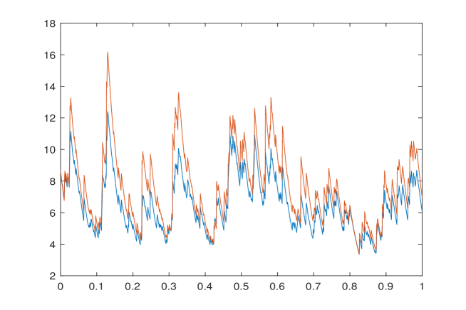
Figure 1: In blue a trajectory of the OU gamma stationary model and in red a trajectory of its TPL extension from the same random drawing. The parameters are $\alpha=25$, $\delta=20$, $\lambda=\theta=0.5$, $\gamma=0.7$.

Another classic application of Lévy driven SDEs is the explicit construction of a stationary process with (quasi) long-range dependence, which can be attained using a superposition of the SDEs (4.1) as explained in Barndorff-Nielsen, (1997), Theorem 4.1 .

4.2 Self-similar TPL processes with independent increments

As shown by Sato, (1991), for all $H>0$ to any self-decomposable distribution $D$ we can associate a self-similar process with Hurst exponent $H$ with independent increments (s.s.i.i.) having $D$ as unit time marginal. Unless $D$ is a stable distribution, such process will not be the same one as the Lévy process with unit time law $D$. As it turns out, when $D$ is TPL all the marginals of the TPL s.s.i.i. process remain TPL and we thus have an explicit representation for its law and Lévy measure.

Proposition 4.3.

Let $H>0$ and $X$ be a TPL$(\gamma,\lambda,\delta,\theta)$ r.v. with $\gamma\in(0,1)$. There exists a stochastically-continuous s.s.i.i. process $X^{H}=(X_{t}^{H})_{t\geq 0}$ of Hurst index $H$ with independent increments such that $X_{1}^{H}$ has the same distribution as $X$, and whose triplet of the integrated semimartingale characteristics is $(0,0,U^{H}(dt,dx))$ with $U^{H}(dt,dx)$ having density

$$u^{H}_{X}(t,x)=\gamma\delta\frac{e^{-\theta t^{-H}x}}{x}E_{\gamma}\left(c_{\gamma,\lambda,\theta}(t^{-H}x)^{\gamma}\right).$$ (4.15)

In particular $X^{H}_{t}$ has $\text{{TPL}}(\gamma,\delta,\lambda t^{H\gamma},\theta t^{-H})$ distribution. Furthermore we have the subordinated representation

$$X^{H}=Y^{H}_{Z}$$ (4.16)

where $Y^{H}$ is the s.s.i.i. process associated to a TPS$(\gamma,\lambda,\theta)$ law which is such that $Y_{t}^{H}$ has TPS$(\gamma,\lambda t^{H\gamma},\theta t^{-H})$ distribution, and $Z$ is a $G(1,\delta)$ independent gamma Lévy process.

Proof.

The existence of $X^{H}$ for a given unit time self-decomposable marginal $X$, and its characterization in terms of the integrated semimartingale characteristic triplet is provided in Sato, (1991). In particular the integrated Lévy measure of $X^{H}$ is absolutely continuous and its density is given by

$$u^{H}_{X}(t,x)=t^{-H}u_{X}(t^{-H}x).$$ (4.17)

Remembering (2.17) and the density (4.15) follows.

To prove the second statement consider the s.s.i.i. process with independent increments $Y_{t}^{H}$ and combine the substitution in (4.17) with the Lévy density (2.12) which determines the integrated Lévy density $u^{H}_{Y}(t,x)$ of $Y_{t}^{H}$ as

$$u^{H}_{Y}(t,x)=\frac{\gamma\lambda t^{-H}}{\Gamma(1-\gamma)}\frac{e^{-\theta t^{-H}x}}{{(xt^{-H})}^{\gamma+1}}\mathds{1}_{\{x>0\}}dx=\frac{\gamma\lambda t^{\gamma H}}{\Gamma(1-\gamma)}\frac{e^{-\theta t^{-H}x}}{{x}^{\gamma+1}}\mathds{1}_{\{x>0\}}dx$$ (4.18)

showing that $Y^{H}_{t}$ has TPS$(\gamma,\lambda t^{H\gamma},\theta t^{-H})$ law. Now using (4.17) in (2.15) implies

$$\phi_{X^{H}}(s)=\phi_{X}(st^{H})=\phi_{Z}(\phi_{Y}(st^{H}))=\phi_{Z}(\phi_{Y^{H}}(s))$$ (4.19)

which terminates the proof. ∎

We observe that as $t\rightarrow\infty$ tempering tends to zero and $X^{H}_{t}$ approaches a large scale PL variable.

Self-similarity is a property which is often observed in financial returns time series. Using additive processes in place of Lévy ones in finance has also benefits for valuation of derivative securities. It is recognized that normalized cumulants of risk-neutral distributions implicit in option prices do not decrease with time to expiration of contracts, or at least not as rapidly as the linear rate of decay predicted by Lévy process, a behaviour which is corrected by removing the assumption of returns stationarity.

5 Multivariate TPL processes

Stochastic self-similarity with respect to the negative binomial subordinator of the gamma process can be exploited for generating multivariate TPL Lévy processes in a natural way, which we illustrate in the following. Multivariate g.i.d. laws are studied in Mittnik and Rachev, (1991): recently, multivariate Mittag-Leffler distributions have been explored in Albrecher et al., (2021) and Khokhlov et al., (2020).

Let $d\in\mathbb{N}$ and $X=(X_{t})_{t\geq 0}$ with $X_{t}=(X^{1}_{t},\ldots,X_{t}^{d})$ be an independent multivariate TPL$(\gamma_{i},\lambda_{i},1,\theta_{i})$ Lévy process i.e. $X$ is such that for all $t$, $X^{i}_{t}$ is independent from $X^{j}_{t}$ whenever $i\neq j$. Let $B^{\pi}$ be a negative binomial process NB$(\pi,\delta,1,\delta)$ independent of $X$. According to Corollary 3.4 the subordinate multivariate Lévy process $X^{\pi}=(X^{\pi}_{t})_{t\geq 0}$ with

$$X^{\pi}_{t}=(X^{\pi,1}_{t},\ldots,X_{t}^{\pi,d}):=(X^{1}_{B^{\pi}_{t}},\ldots,X^{d}_{B^{\pi}_{t}})$$ (5.1)

is such that $X^{\pi,i}=(X^{\pi,i})_{t\geq 0}$ has $\text{TPL}(\gamma_{i},\lambda_{i}\pi^{-1},\delta,\theta_{i})$ law. Therefore $X^{\pi}$ is a multivariate Lévy process with correlated TPL marginals, conditionally independent on $B^{\pi}$, and the success probability $\pi$ plays the role of a dependence parameter with the degenerate case $\pi=1$ amounting to the independent case ($B^{\pi}$ being pure drift in such a case). According to the general properties of TPL laws illustrated in Section 2, depending on whether $\gamma_{i}\in(0,1]$ or $\gamma_{i}<0$ the marginal processes can be either infinite activity with nonintegrable Lévy marginal measure and absolutely-continuous law, or CPPs, whose law has a point mass in zero.

A useful alternative representation of $X^{\pi}$ can also be provided. By virtue of Remark 3.1 for all $i=1,\ldots,d$, we can interpret the marginal processes $X^{i}$ as $X^{i}=Y^{i}_{Z^{i}}$, for two independent multivariate Lévy processes $Y^{i}$ and $Z^{i}$, where $Y^{i}$ is a TPS$(\gamma_{i},1,\theta_{i})$ process and $Z^{i}$ is a gamma $G(\lambda_{i},1)$ process independent of $Y^{i}$ and therefore

$$X_{t}=^{d}\left(Y^{1}_{Z^{1}_{t}},\ldots,Y^{d}_{Z^{d}_{t}}\right).$$ (5.2)

Choosing further $Y^{j}$, $Y^{i}$ and $Z^{i}$, $Z^{j}$ to be independent whenever $i\neq j$, we can introduce two independent multivariate Lévy processes $Y=(Y^{1}_{t},\ldots,Y_{t}^{d})$ and $Z=(Z^{1}_{t},\ldots,Z_{t}^{d})$ with independent marginals and (5.2) has the interpretation of a multivariate subordination of $Y$ to $Z$, as detailed Barndorff-Nielsen et al., (2001). We shall denote multivariate subordination in the same way as the standard one, and therefore (5.2) implicates $X=Y_{Z}$. Furthermore, by Proposition 3.3 it holds

$$X^{\pi}_{t}=^{d}\left(\left(Y^{1}_{{Z^{1}}}\right)_{B^{\pi}_{t}},\ldots,\left(Y^{d}_{{Z^{d}}}\right)_{B^{\pi}_{t}}\right)=^{d}\left(Y^{1}_{Z^{\pi,1}_{t}},\ldots,Y^{d}_{Z^{\pi,d}_{t}}\right),$$ (5.3)

where $Z^{\pi,i}=Z^{i}_{B^{\pi}}$ are $G(\lambda_{i}\pi^{-1},\delta)$ processes, making $Z^{\pi}=(Z^{\pi}_{t})_{t\geq 0}$ given by

$$Z^{\pi}_{t}=(Z^{\pi,1}_{t},\ldots,Z^{\pi,d}_{t})$$ (5.4)

into a multivariate gamma subordinator with dependent marginals. Therefore, $X^{\pi}$ enjoys the multivariate subordinated representation

$$X^{\pi}=Y_{Z^{\pi}}.$$ (5.5)

In order to further investigate $X^{\pi}$ we first compute the Lévy density of $Z^{\pi}$, which is also of independent interest. Notice that unlike $X^{\pi}$, $Z^{\pi}$ is a multivariate process attained by ordinary subordination.

Proposition 5.1.

The process $Z^{\pi}$ is a multivariate Lévy subordinator with zero drift and Lévy measure

$$\rho^{\pi}(dt_{1}\ldots dt_{d})=\delta\left(\prod_{i=1}^{d}\frac{e^{-t_{i}\pi/\lambda_{i}}-e^{-t_{i}/\lambda_{i}}}{t_{i}}dt_{1}\ldots dt_{d}+\sum_{i=1}^{d}\frac{e^{-t_{i}/\lambda_{i}}}{t_{i}}dt_{i}\right)\mathds{1}_{\{t_{i}>0\}}.$$ (5.6)

Proof.

By using the p.m.f. (3.24) one can show that the Lévy measure $r^{\pi}$ of $B^{\pi}$ is (e.g. Kozubowski and Podgórski, 2009)

$$r^{\pi}=\delta\sum_{k=1}^{\infty}\frac{(1-\pi)^{k}}{k}\delta_{k},$$ (5.7)

where $\delta_{k}$ is the Dirac measure concentrated in $k$. With a slight abuse of notation, we write the multivariate Lévy density of $Z$ as

$$u_{Z}(dt_{1}\ldots dt_{d})=\sum_{i=1}^{d}\frac{e^{-t_{i}/\lambda_{i}}}{t_{i}}\mathds{1}_{\{t_{i}>0\}}dt_{i}$$ (5.8)

and the multivariate independent gamma law $\mu^{Z}_{t}$ as

$$\mu^{Z}_{t}=\prod_{i=1}^{d}f_{Z^{i}}(t_{i};\lambda_{i},t)dt_{1}\ldots dt_{d}=\prod_{i=1}^{d}\frac{t_{i}^{t-1}}{\Gamma(t)\lambda_{i}^{t}}e^{-t_{i}/\lambda_{i}}\mathds{1}_{\{t_{i}>0\}}dt_{1}\ldots dt_{d}.$$ (5.9)

Using the multivariate version of the (ordinary) subordination integral (2.8) (Sato, 1999, Chapter 30) with triplets $(0,0,u_{Z}(dt_{1}\ldots dt_{d}))$ and $(0,\delta,r^{\pi})$, and probability law $\mu^{Z}_{t}$ we have, applying monotone convergence to interchange integration in $du$ and the series

$$\rho^{\pi}(dt_{1}\ldots dt_{d}) =\delta\sum_{k=1}^{\infty}\frac{(1-\pi)^{k}}{k}\int_{(0,\infty)}\left(\prod_{i=1}^{d}\frac{t_{i}^{u-1}}{\Gamma(u)\lambda_{i}^{u}}e^{-t_{i}/\lambda_{i}}dt_{1}\ldots dt_{d}\right)\delta_{k}(du)+\delta\sum_{i=1}^{d}\frac{e^{-t_{i}/\lambda_{i}}}{t_{i}}\mathds{1}_{\{t_{i}>0\}}dt_{i}$$

$$=\delta\prod_{i=1}^{d}\frac{e^{-t_{i}/\lambda_{i}}}{t_{i}}\mathds{1}_{\{t_{i}>0\}}\sum_{k=1}^{\infty}\left(\frac{t_{i}(1-\pi)}{\lambda_{i}}\right)^{k}\frac{1}{k!}dt_{1}\ldots dt_{d}+\delta\sum_{i=1}^{d}\frac{e^{-t_{i}/\lambda_{i}}}{t_{i}}\mathds{1}_{\{t_{i}>0\}}dt_{i}$$

$$=\delta\prod_{i=1}^{d}\frac{e^{-t_{i}/\lambda_{i}}}{t_{i}}\mathds{1}_{\{t_{i}>0\}}\left(\frac{e^{t_{i}(1-\pi)/\lambda_{i}}}{t_{i}}-1\right)dt_{1}\ldots dt_{d}+\delta\sum_{i=1}^{d}\frac{e^{-t_{i}/\lambda_{i}}}{t_{i}}\mathds{1}_{\{t_{i}>0\}}dt_{i},$$ (5.10)

which proves (5.6). ∎

Together with the foregoing discussion, Proposition 5.1 allows the identification of the Lévy structure of $X^{\pi}$.

Theorem 5.2.

The process $X^{\pi}$ is a multidimensional Lévy subordinator with multivariate characteristic exponent, for Re$(s_{i})>0$, $i=1,\ldots,d$ given by

$$\phi_{X^{\pi}}(s_{1},\ldots,s_{d})=\delta\log\left(1+\frac{1}{\pi}-\frac{1}{\pi}\prod_{i=1}^{d}\left(1+\text{{sgn}}(\gamma_{i})\lambda_{i}((\theta_{i}+s_{i})^{\gamma_{i}}-\theta_{i}^{\gamma_{i}})\right)\right).$$ (5.11)

Furthermore $X^{\pi}$ has zero drift, and Lévy density

$$u^{\pi}_{X}(x_{1},\ldots,x_{d})=\delta\sum_{A\subseteq\{1,\ldots,d\}}(-1)^{|A|}\prod_{i\in A}|\gamma_{i}|\frac{e^{-\theta_{i}x_{i}}}{x_{i}}\left(E_{|\gamma_{i}|}\left(c_{{\gamma_{i}},\lambda_{i},\theta_{i}}x_{i}^{|\gamma_{i}|}\right)-\mathds{1}_{\{\text{{sgn}}(\gamma_{i})=-1\}}\right)$$

$$\phantom{xxxxxxx}\ \times\prod_{i\in A^{c}}|\gamma_{i}|\frac{e^{-\theta_{i}x_{i}}}{x_{i}}\left(E_{|\gamma_{i}|}\left(c_{{\gamma_{i}},\pi\lambda_{i},\theta_{i}}x_{i}^{|\gamma_{i}|}\right)-\mathds{1}_{\{\text{{sgn}}(\gamma_{i})=-1\}}\right)$$

$$\phantom{xxxxxxx}+\delta\sum_{i=1}^{d}|\gamma_{i}|\frac{e^{-\theta_{i}x_{i}}}{x_{i}}\left(E_{|\gamma_{i}|}\left(c_{{\gamma_{i}},\lambda_{i},\theta_{i}}x_{i}^{|\gamma_{i}|}\right)-\mathds{1}_{\{\text{{sgn}}(\gamma_{i})=-1\}}\right)$$ (5.12)

for $x_{i}>0$, and zero otherwise, with $(\gamma_{i},\lambda_{i},\delta_{i},\theta_{i})\in S$ for all $i=1,\ldots,d$, where the constants $c_{{\gamma_{i}},\lambda_{i},\theta_{i}}$ and $c_{{\gamma_{i}},\pi\lambda_{i},\theta_{i}}$ are given by (2.18) with the appropriate parameter modifications.

Proof.

By definition of $X^{\pi}$ and independence

$$\phi_{X^{\pi}}(s_{1},\ldots,s_{d})=\phi_{B^{\pi}}(\phi_{X}(s_{1},\ldots,s_{d}))=\phi_{B^{\pi}}(\phi_{X}(s_{1})\ldots\phi_{X}(s_{d}))$$ (5.13)

and (5.11) is then clear from (2.2) and (3.22).

We indicate with $\mu^{Y}_{t_{1},\ldots,t_{n}}$ the probability law of the random vector $(Y^{1}_{t_{1}},\ldots Y^{d}_{t_{d}})$ and by $\rho^{\pi}$ the Lévy measure of $Z^{\pi}$ given in Proposition 5.1. By virtue of (5.5) we can apply Barndorff-Nielsen et al., (2001) Theorem 3.3, and we see that $X^{\pi}$ has Lévy triplet $(0,0,\eta^{\pi})$ with

$$\eta^{\pi}(B)=\int_{\mathbb{R}_{+}^{d}}\mu^{Y}_{t_{1},\ldots,t_{n}}(B)\rho^{\pi}(dt_{1}\ldots dt_{n})$$ (5.14)

for Borel sets $B\subseteq\mathbb{R}^{d}_{+}$. Now by independence we have the product measure

$$\mu^{Y}_{t_{1},\ldots,t_{n}}=\prod_{i=1}^{d}\mu^{Y^{i}}_{t_{i}}$$ (5.15)

where $\mu^{Y^{i}}_{t}$ indicates the law of $Y_{t}^{i}$. Substituting (5.6) and (5.15) in (5.14) and using Proposition 2.1 in the second summand of (5.6), we obtain the density for $x_{i}>0$,

$$u^{\pi}_{X}(x_{1},\ldots,x_{d})=\delta\int_{\mathbb{R}_{+}^{d}}\prod_{i=1}^{d} f_{Y^{i}}(x_{i};\gamma_{i},\theta_{i},t_{i})\frac{e^{-t_{i}\pi/\lambda_{i}}-e^{-t_{i}/\lambda_{i}}}{t_{i}}dt_{1}\ldots dt_{d}$$

$$+\delta\sum_{i=1}^{d}|\gamma_{i}|\frac{e^{-\theta_{i}x_{i}}}{x_{i}}\left(E_{|\gamma_{i}|}\left(c_{{\gamma_{i}},\lambda_{i},\theta_{i}}x_{i}^{|\gamma_{i}|}\right)\mathds{1}_{\{\text{{sgn}}(\gamma_{i})=-1\}}\right)$$ (5.16)

where $f_{Y^{i}}(x_{i};\gamma_{i},\theta_{i},t_{i})$ is given by (2.14) if $\gamma_{i}\in(0,1)$, or the absolutely continuous part of (2.1) if $\gamma_{i}<0$. Now observe the additive expansion:

$$\prod_{i=1}^{d}\frac{e^{-t_{i}\pi/\lambda_{i}}-e^{-t_{i}/\lambda_{i}}}{t_{i}}=\sum_{A\subseteq\{1,\ldots,d\}}(-1)^{|A|}\exp\left(-\sum_{i\in A}\frac{t_{i}}{\lambda_{i}}-\pi\sum_{i\in A^{c}}\frac{t_{i}}{\lambda_{i}}\right)\prod_{i=1}^{d}t_{i}^{-1}$$ (5.17)

where $|A|$ denotes the cardinality of the subset $A$. In view of (5.17) we can rewrite the first term in (5) as

$$\int_{\mathbb{R}_{+}^{d}} \prod_{i=1}^{d}f_{Y^{i}}(x_{i};\gamma_{i},\theta_{i},t_{i})\frac{e^{-t_{i}\pi/\lambda_{i}}-e^{-t_{i}/\lambda_{i}}}{t_{i}}dt_{1}\ldots dt_{d}$$

$$=\sum_{A\subseteq\{1,\ldots,d\}}(-1)^{|A|}\left(\prod_{i\in A}\int_{\mathbb{R}_{+}}f_{Y^{i}}(x_{i};\gamma_{i},\theta_{i},t_{i})\frac{e^{-t_{i}/\lambda_{i}}}{t_{i}}dt_{i}\prod_{i\in A^{c}}\int_{\mathbb{R}_{+}}f_{Y^{i}}(x_{i};\gamma_{i},\theta_{i},t_{i})\frac{e^{-\pi t_{i}/\lambda_{i}}}{t_{i}}dt_{i}\right)$$ (5.18)

with the product term corresponding to the empty set being one. Replicating the integrations in Proposition 2.1 we finally arrive at (5.2). ∎

The Lévy measure of $X^{\pi}$ thus decomposes in an independent multivariate TPL measure plus a combinatorial expression of one-dimensional TPL Lévy measures depending on $\pi$ accounting for the dependence across the marginals, which increasingly gains weight as $\pi$ decreases from one to zero. In the case $\gamma_{i}=1$ for all $i$ we notice from (5.11) that $X^{\pi}_{t}$ follows the multivariate gamma law discussed in Gaver, (1970) and generalizing Kibble, (1941), which is widely popular for applications.

6 Potential for statistical anti-fraud applications

One major motivation for our interest in the univariate TPS and TPL laws is their ability to model international trade data, with particular reference to imports into (and exports from) the Member States of the European Union (EU). Due to the combination of economic activities and normative constraints, the empirical distribution of traded quantities and traded values in imports and exports is often markedly skewed with heavy tails, featuring a large number of rounding errors in small-scale transactions due to data registration problems, and structural zeros arising because of confidentiality issues related to national regulations within the EU. While such features are not easy to be combined into a single statistical model, Barabesi et al., 2016b and Barabesi et al., 2016a show that in the univariate case both the TPS and TPL distributions do provide reliable models for the monthly aggregates of import quantities of several products of interest.

The main operational target of the research line on international trade data sketched above is the construction of sound statistical methods for the detection of customs frauds, such as the under-valuation of import duties, and the investigation of other trade-related infringements, such as money laundering and circumvention of regulatory measures. In this framework flexible statistical models that can accurately describe the distribution of traded quantities and values for a very large number of products is of paramount importance for several reasons. Firstly, such models could provide direct support to policy makers, e.g. in the form of tools for monitoring the effect of policy measures and for providing factual background for the official communications on trade policy. Another goal, which is perhaps even more prominent from a statistical standpoint, is their use in model-based assessments of the performance of methods used for finding relevant signals of potential fraud.

Most of the fraud detection tools adopted in the context of international trade look for anomalies in the data. Therefore, they typically make use of outlier detection methods for multivariate and regression data, such as those described in Cerioli, (2010) and Perrotta et al., 2020a , as well as of robust clustering techniques (see e.g. Cerioli and Perrotta,, 2014). All of these techniques assume that the available data have been generated by an appropriate contamination model, which in the context of international trade typically involves at least two variables, in view of the basic economic relationship that yields the value of an individual import (export) transaction as the product of the traded amount and the unit price. Any parameter of the distribution that models the “genuine” part of the data must then be estimated in a robust way, in order to avoid the well-known masking and swamping effects due to the anomalies themselves (see e.g. Cerioli et al., 2019b, ). Relying on the theory of robust high-breakdown estimation, that typically assumes elliptical symmetry of the uncontaminated data-generation process, it is very difficult to derive analytical results for such methods when skewed distributions should be used for realistic modeling of economic processes. The available methods need thus to be compared, evaluated and eventually tuned on a large number of data sets artificially generated with known statistical properties, which must reflect the distributions observed in real-world trade data. Cerioli and Perrotta, (2014) show a first attempt in this direction under a rather specialized ad-hoc model. The class of multivariate TPL processes described in Section 5 provides instead a very natural and general reference model, extending the framework suggested by Barabesi et al., 2016a to the simultaneous description of (at least) traded quantities and traded values. Reliable inferential results for anti-fraud diagnostics computed on trade data could then be obtained by simulation from this class of processes following a model-based Monte Carlo scheme, in the spirit e.g. of Besag and Diggle, (1977), Bladt and Sørensen, (2014) and Guerrier et al., (2019).

A similar requirement holds for an alternative approach to fraud detection which has recently attracted considerable attention also in international trade and which rests on the development of powerful and accurate conformance tests of Benford’s law (Barabesi et al., 2018b, ; Cerioli et al., 2019a, ; Barabesi et al.,, 2021). This approach aims at unveiling serial fraudsters and has proven to be especially effective for the analysis of individual customs declarations, instead of monthly aggregates of them. A variety of statistical procedures are compared by Cerioli et al., 2019a and Barabesi et al., (2021, Section 7.2) through a bootstrap algorithm that generates pseudo-observations mimicking a national database of one calendar-year customs declarations, after appropriate anonymization that makes it impossible to infer the features of individual operators. The class of multivariate TPL processes can again provide a suitable reference framework for such comparisons when a model-based approach replicating international trade conditions is deemed desirable.

Figure 2 displays one sample of 5.000 observations from a bivariate TPL process simulated using representation (5.3). The parameters of the marginal processes are $\gamma_{1}=\gamma_{2}=-2.2$, $\lambda_{1}=\lambda_{2}=10$, $\theta_{1}=\theta_{2}=0.5$, while $\delta=1$ and $\pi=0.01$ is the success probability relating $X^{\pi,1}$ and $X^{\pi,2}$. The visual similarity between the simulated scatter and the scatter shown in Perrotta et al., 2020b (, Section 4, p. 10) for a homogeneous sample from a fraud-sensitive commodity is striking and confirms the potential of multivariate TPL processes for describing the joint distribution of relevant variables arising in international trade. Therefore, we argue that suitably tuned versions of $X^{\pi}$ could lead to reliable simulation inference for outlier labeling rules and other anti-fraud diagnostics in trade data structures, when the distributional assumption of symmetry for individual uncontaminated observations, typically implied by such methods, is not met. This is an important research goal for anti-fraud applications and international trade analysis, also foreseen in Barabesi et al., (2021, Section 7.2).

Figure 2: Simulated sample from a multivariate TPL process with $d=2$, $\delta=1$, $\pi=0.01$ and marginal parameters given in the text.

Acknowledgments

This research has financially been supported by the Programme “FIL-Quota Incentivante” of the University of Parma and co-sponsored by Fondazione Cariparma. The authors thank Peter Carr and Luca Pratelli for the helpful discussions on a previous draft. They are also grateful to Domenico Perrotta and Francesca Torti of the Joint Research Centre of the European Commission for inspiring the anti-fraud applications of the tempered processes described in this work.

References

- Albrecher et al., (2021) Albrecher, H., Bladt, M., and Bladt, M. (2021). Multivariate matrix Mittag–Leffler distributions. Annals of the Institute of Statistical Mathematics, 73:369–394.
- Barabesi, (2020) Barabesi, L. (2020). The computation of the probability density and distribution functions for some families of random variables by means of the Wynn- accelerated Post-Widder formula. Communications in Statistics – Simulation and Computation, 49:1331–1351.
- (3) Barabesi, L., Becatti, C., and Marcheselli, M. (2018a). The tempered discrete Linnik distribution. Statistical Methods and Applications, 27:45–68.
- (4) Barabesi, L., Cerasa, A., Cerioli, A., and Perrotta, D. (2016a). A new family of tempered distributions. Electronic Journal of Statistics, 10:3871–3893.
- (5) Barabesi, L., Cerasa, A., Cerioli, A., and Perrotta, D. (2018b). Goodness-of-fit testing for the Newcomb-Benford law with application to the detection of customs fraud. Journal of Business and Economic Statistics, 36:346–358.
- Barabesi et al., (2021) Barabesi, L., Cerasa, A., Cerioli, A., and Perrotta, D. (2021). On characterizations and tests of Benford’s law. Journal of the American Statistical Association. DOI: 10.1080/01621459.2021.1891927.
- (7) Barabesi, L., Cerasa, A., Perrotta, D., and Cerioli, A. (2016b). Modeling international trade data with the Tweedie distribution for anti-fraud and policy support. European Journal of Operational Research, 248:1031–1043.
- Barabesi and Pratelli, (2014) Barabesi, L. and Pratelli, L. (2014). A note on a universal random variate generator for integer-valued random variables. Statistics and Computing, 24:589–596.
- Barabesi and Pratelli, (2015) Barabesi, L. and Pratelli, L. (2015). Universal methods for generating random variables with a given characteristic function. Journal of Statistical Computation and Simulation, 85:1679–1691.
- Barabesi and Pratelli, (2019) Barabesi, L. and Pratelli, L. (2019). On the properties of a Takács distribution. Statistics and Probability Letters, 148:66–73.
- Barndorff-Nielsen, (1997) Barndorff-Nielsen, O. E. (1997). Processes of normal inverse Gaussian type. Finance and Stochastics, 2:41–68.
- Barndorff-Nielsen, (2000) Barndorff-Nielsen, O. E. (2000). Probability densities and Lévy densities. Technical Report MPS–RR 2000–18, Aarhus University, Centre for Mathematical Physics and Stochastics (MaPhySto).
- Barndorff-Nielsen et al., (2002) Barndorff-Nielsen, O. E., Nicolato, E., and Shephard, N. (2002). Some recent developments in stochastic volatility modelling. Quantitative Finance, 2:11–23.
- Barndorff-Nielsen et al., (2001) Barndorff-Nielsen, O. E., Pedersen, J., and Sato, K. (2001). Multivariate subordination, self-decomposability and stability. Advances in Applied Probability, 33:160–187.
- Barndorff-Nielsen and Shephard, (2001) Barndorff-Nielsen, O. E. and Shephard, N. (2001). Non-Gaussian Ornstein–Uhlenbeck-based models and some of their uses in financial economics. Journal of the Royal Statistical Society: Series B, 63:167–241.
- Besag and Diggle, (1977) Besag, J. and Diggle, P. (1977). Simple Monte Carlo tests for spatial pattern. Journal of the Royal Statistical Society. Series C (Applied Statistics), 26:327–333.
- Bladt and Sørensen, (2014) Bladt, M. and Sørensen, M. (2014). Simple simulation of diffusion bridges with application to likelihood inference for diffusions. Bernoulli, 20:645–675.
- Boyarchenko and Levendorskiï, (2000) Boyarchenko, S. I. and Levendorskiï, S. Z. (2000). Option pricing for truncated Lévy processes. International Journal of Theoretical and Applied Finance, 3:549–552.
- Carr et al., (2002) Carr, P., Geman, H., Madan, D. B., and Yor, M. (2002). The fine structure of asset returns: an empirical investigation. Journal of Business, 75:305–332.
- Cerioli, (2010) Cerioli, A. (2010). Multivariate outlier detection with high-breakdown estimators. Journal of the American Statistical Association, 105:147–156.
- (21) Cerioli, A., Barabesi, L., Cerasa, A., Menegatti, M., and Perrotta, D. (2019a). Newcomb-Benford law and the detection of frauds in international trade. Proceedings of the National Academy of Sciences, 116:106–115.
- (22) Cerioli, A., Farcomeni, A., and Riani, M. (2019b). Wild adaptive trimming for robust estimation and cluster analysis. Scandinavian Journal of Statistics, 46:235–256.
- Cerioli and Perrotta, (2014) Cerioli, A. and Perrotta, D. (2014). Robust clustering around regression lines with high density regions. Advances in Data Analysis and Classification, 8:5–26.
- Christoph and Schreiber, (2001) Christoph, G. and Schreiber, K. (2001). Positive Linnik and discrete Linnik distributions. In Balakrishnan, N., Ibragimov, I. V., and Nevzorov, V. B., editors, Asymptotic Methods in Probability and Statistics with Applications, pages 3–17. Birkhäuser, Boston.
- Fallahgoul and Loeper, (2021) Fallahgoul, H. and Loeper, G. (2021). Modelling tail risk with tempered stable distributions: an overview. Annals of Operations Research, 299:1253–1280.
- Fontaine et al., (2020) Fontaine, S., Yang, Y., Qian, W., Gu, Y., and Fan, B. (2020). A unified approach to sparse Tweedie modeling of multisource insurance claim data. Technometrics, 62:339–356.
- Gaver, (1970) Gaver, D. P. (1970). Multivariate gamma distributions generated by mixture. Sankhy, Series A, pages 123–126.
- Gorenflo et al., (2020) Gorenflo, R., Kilbas, A. A., Mainardi, F., and Rogosin, S. (2020). Mittag-Leffler Functions, Related Topics and Applications. Second Edition. Springer, Berlin.
- Grabchak, (2016) Grabchak, M. (2016). Tempered Stable Distributions: Stochastic Models for Multiscale Processes. Springer, Cham.
- Grabchak, (2019) Grabchak, M. (2019). Rejection sampling for tempered Lévy processes. Statistics and Computing, 29:549–558.
- Guerrier et al., (2019) Guerrier, S., Dupuis-Lozeron, E., Ma, Y., and Victoria-Feser, M.-P. (2019). Simulation-based bias correction methods for complex models. Journal of the American Statistical Association, 114:146–157.
- Haubold et al., (2011) Haubold, H. J., Mathai, A. M., and Saxena, R. K. (2011). Mittag-Leffler functions and their applications. Journal of Applied Mathematics. Article ID 298628.
- Hubalek and Sgarra, (2006) Hubalek, F. and Sgarra, C. (2006). Esscher transforms and the minimal entropy martingale measure for exponential Lévy models. Quantitative Finance, 6:125–145.
- Jurek and Vervaat, (1983) Jurek, Z. J. and Vervaat, W. (1983). An integral representation for selfdecomposable Banach space valued random variables. Zeitschrift für Wahrscheinlichkeitstheorie und verwandte Gebiete, 62:247–262.
- Kalashnikov, (1997) Kalashnikov, V. V. (1997). Geometric Sums: Bounds for Rare Events with Applications. Springer, Dordrecht.
- Khalin and Postnikov, (2020) Khalin, A. A. and Postnikov, E. B. (2020). A wavelet-based approach to revealing the Tweedie distribution type in sparse data. Physica A, 553:124653.
- Khokhlov et al., (2020) Khokhlov, Y., Korolev, V., and Zeifman, A. (2020). Multivariate scale-mixed stable distributions and related limit theorems. Mathematics, 8:749.
- Kibble, (1941) Kibble, W. F. (1941). A two-variate gamma type distribution. Sankhy, 5:137–150.
- Klebanov et al., (1985) Klebanov, L. B., Maniya, G. M., and Melamed, I. A. (1985). A problem of Zolotarev and analogs of infinitely divisible and stable distributions in a scheme for summing a random number of random variables. Theory of Probability and its Applications, 29:791–794.
- Koponen, (1995) Koponen, I. (1995). Analytic approach to the problem of convergence of truncated Lévy flights towards the Gaussian stochastic process. Physical Review E, 52:1197–1199.
- Korolev et al., (2020) Korolev, V., Gorshenin, A., and Zeifman, A. (2020). On mixture representations for the generalized Linnik distribution and their applications in limit theorems. Journal of Mathematical Sciences, 246:503–518.
- Kozubowski et al., (2006) Kozubowski, T. J., Meerschaert, M. M., and Podgórski, K. (2006). Fractional Laplace motion. Advances in Applied Probability, 38:451–464.
- Kozubowski and Podgórski, (2009) Kozubowski, T. J. and Podgórski, K. (2009). Distributional properties of the negative binomial Lévy process. Probability and Mathematical Statistics, 29:43–71.
- Kozubowski and Rachev, (1999) Kozubowski, T. J. and Rachev, S. T. (1999). Univariate geometric stable laws. Journal of Computational Analysis and Applications, 1:177–217.
- (45) Kumar, A., Maheshwari, A., and Wylomanska, A. (2019a). Linnik Lévy process and some extensions. Physica A, 529:121539.
- (46) Kumar, A., Upadhye, N. S., Wylomanska, A., and Gajda, J. (2019b). Tempered Mittag-Leffler Lévy processes. Communications in Statistics – Theory and Methods, 48:396–411.
- Kumar and Verma, (2020) Kumar, A. and Verma, H. (2020). Potential theory of normal tempered stable process. Technical Report 2004.02267, arXiv.
- Leonenko et al., (2021) Leonenko, N., Macci, C., and Pacchiarotti, B. (2021). Large deviations for a class of tempered subordinators and their inverse processes. Proceedings of the Royal Society of Edinburgh. Section A: Mathematics. In press.
- Lin, (1994) Lin, G. D. (1994). Characterizations of the Laplace and related distributions via geometric compound. Sankhy, Series A, 56:1–9.
- Lin, (1998) Lin, G. D. (1998). A note on the Linnik distributions. Journal of Mathematical Analysis and Applications, 217:701–706.
- Linnik, (1963) Linnik, Y. V. (1963). Linear forms and statistical criteria, I, II. Selected Translations in Mathematical Statistics and Probability, 3:1–90.
- Ma et al., (2018) Ma, R., Yan, G., and Hasan, M. T. (2018). Tweedie family of generalized linear models with distribution-free random effects for skewed longitudinal data. Statistics in Medicine, 37:3519–3532.
- Mantegna and Stanley, (1994) Mantegna, R. N. and Stanley, H. E. (1994). Stochastic process with ultraslow convergence to a Gaussian: the truncated Lévy flight. Physical Review Letters, 73:2946–2949.
- Mathai and Haubold, (2008) Mathai, A. M. and Haubold, H. J. (2008). Special Functions for Applied Scientists. Springer, New York.
- Mittnik and Rachev, (1991) Mittnik, S. and Rachev, S. T. (1991). Alternative multivariate stable distributions and their applications to financial modeling. In Cambanis, S., Samorodnitsky, G., and Taqqu, M. S., editors, Stable Processes and Related Topics, pages 107–119. Birkäuser, Boston.
- Pakes, (1998) Pakes, A. G. (1998). Mixture representations for symmetric generalized Linnik laws. Statistics and Probability Letters, 37:213–221.
- (57) Perrotta, D., Cerasa, A., Torti, F., and Riani, M. (2020a). The robust estimation of monthly prices of goods traded by the European Union. Technical Report KJ-NA-30188-EN-N (online), Publications Office of the European Union, Luxembourg. DOI: 10.2760/635844 (online).
- (58) Perrotta, D., Checchi, E., Torti, F., Cerasa, A., and Arnes Novau, X. (2020b). Addressing price and weight heterogeneity and extreme outliers in surveillance data. Technical Report KJ-NA-30431-EN-N (online), Publications Office of the European Union, Luxembourg. DOI: 10.2760/817681 (online).
- Pillai, (1990) Pillai, R. N. (1990). On Mittag-Leffler functions and related distributions. Annals of the Institute of Statistical Mathematics, 42:157–161.
- Prabhakar, (1971) Prabhakar, T. R. (1971). A singular integral equation with a generalized Mittag Leffler function in the kernel. Yokohama Mathematical Journal, 19:7–15.
- Sandhya and Pillai, (1999) Sandhya, E. and Pillai, R. N. (1999). On geometric infinite divisibility. Journal of the Kerala Statistical Association, 10:1–7. Retrivable at: arXiv:1409.4022.
- Sato, (1991) Sato, K. (1991). Self-similar processes with independent increments. Probability Theory and Related Fields, 89:285–300.
- Sato, (1999) Sato, K. (1999). Lévy Processes and Infinitely Divisible Distributions. Cambridge University Press, Cambridge.
- Schilling et al., (2012) Schilling, R. L., Song, R., and Vondraček, Z. (2012). Bernstein Functions: Theory and Applications. Second Edition. De Gruyter, Berlin.
- Steutel and Van Harn, (2004) Steutel, F. W. and Van Harn, K. (2004). Infinite Divisibility of Probability Distributions on the Real Line. Dekker, New York.
- Wolfe, (1982) Wolfe, S. J. (1982). On a continuous analogue of the stochastic difference equation . Stochastic Processes and Their Applications, 12:301–312.
- Wright, (1935) Wright, E. M. (1935). The asymptotic expansion of the generalized hypergeometric function. Journal of the London Mathematical Society, 10:286–293.