The $pp\to W(\to l\nu)+\gamma$ process at next-to-next-to-leading order

Abstract

We present details of the calculation of the $pp\to W(\to l\nu)\gamma$ process at next-to-next-to-leading order in QCD, calculated using the jettiness slicing method. The calculation is based entirely on analytic amplitudes. Because of the radiation zero, the NLO QCD contribution from the $gq$ channel is as important as the contribution from the Born $q\bar{q}$ process, disrupting the normal counting of leading and sub-leading contributions. We also assess the importance of electroweak (EW) corrections, including the EW corrections to both the six-parton channel $0\to\bar{u}d\nu e^{+}\gamma g$ and the five-parton channel $0\to\bar{u}d\nu e^{+}\gamma$. Previous experimental results have been shown to agree with theoretical predictions, taking into account the large experimental errors. With the advent of run II data from the LHC, the statistical errors on the data will decrease, and will be competitive with the error on theoretical predictions for the first time. We present numerical results for $\sqrt{s}=7$ and $13$ TeV. Analytic results for the one-loop six-parton QCD amplitude and the tree-level seven-parton QCD amplitude are presented in appendices.

1 Introduction

The process $pp\to W(\to l\nu)+\gamma$ occupies a special place amongst the high-energy processes sensitive to triple coupling of three vector bosons. Of all the vector-boson pair-production processes which are sensitive to the triple gauge boson coupling, it has the largest cross section. The discovery, some forty years ago, of the radiation zero Mikaelian:1979nr ; Brown:1979ux in the leading-order prediction for this process indicates a high amount of destructive interference between the contributing sub-amplitudes. This characteristic interference pattern, even though attenuated by higher-order corrections, still implies that this process is a particularly sensitive test of the gauge structure, allowing incisive probes of the three-boson coupling.

On the theoretical side, early calculations of the QCD radiative corrections Smith:1989xz ; Ohnemus:1992jn ; Baur:1993ir showed that the radiation zero, which manifests itself in $pp$ collisions as a dip in the centre-of-mass rapidity of the photon at $y_{\gamma}^{*}=0$, persists in the NLO theory, but with diminished importance. With the advent of spinor techniques, compact analytic expressions became available for the one-loop $u\bar{d}\to W\gamma$ amplitudes Dixon:1998py . For a review of the status at the dawn of the LHC era, see Campbell:2011bn where results for NLO processes implemented in MCFM are reported. More recently NLO $W\gamma$ production in hadronic collisions has been interfaced to a shower generator according to the POWHEG prescription in such a way that the contribution arising from hadron fragmentation into photons is fully modelled Barze:2014zba .

The large correction in passing from leading order to next-to-leading order, caused by the radiation zero, hints at the potential importance of a NNLO calculation. A NNLO calculation has been achieved in refs. Grazzini:2016hai ; Grazzini:2015nwa using a $q_{T}$ slicing method. Subsequently this process has been treated in a unified framework by the MATRIX program Grazzini:2017mhc , where the matrix elements are calculated using the OpenLoops procedure Cascioli:2011va . A further development is the calculation of electroweak effects Accomando:2001fn and their combination with both NLO QCD calculations Denner:2014bna and NNLO QCD calculations Kallweit:2019zez . The results presented in this paper are similar in spirit, but different in detail from the results of refs. Grazzini:2017mhc ; Kallweit:2019zez :

1. Instead of the $q_{T}$ slicing method, we use the $N$-jettiness slicing method, which has been successfully implemented in MCFM for the following processes, $pp\to H+X$, $pp\to W^{\pm}$, $pp\to Z$, $pp\to WH$, $pp\to ZH$, $pp\to\gamma\gamma$ Boughezal:2016wmq , $pp\to Z\gamma$ Campbell:2017aul , $pp\to Z+$ jet Boughezal:2015ded , $pp\to H+$ jet Campbell:2019gmd .

2. All amplitudes and hence matrix elements entering our NNLO QCD calculation are implemented using analytic formulae. We believe this will have benefits for both the stability and speed of the code. Thus for example our NNLO calculation needs the one-loop contribution to the six-parton process. The first complete one-loop analytic result for this process is presented in an appendix to this paper. Part of this result is derivable from Ref. Bern:1997sc . As usual these one-loop processes are calculated using analytic unitarity methods Britto:2004nc ; Forde:2007mi ; Mastrolia:2009dr . They are further manipulated and simplified by means of high-precision floating-point reconstruction DeLaurentis:2019phz .

3. Our code can accommodate a non-diagonal CKM matrix. While this is known to give quite small modifications, its inclusion eliminates an entirely avoidable theoretical error.

4. We have studied the impact of electroweak corrections, including for the first time the $O(\alpha_{s})$ gluon-quark initiated process, which is numerically as important as the quark-antiquark initiated process.

On the experimental side, the $W\gamma$ process was first observed at the Tevatron Abe:1994fx ; D0:1995mca with a handful of events and larger-statistics studies were later performed both by CDF Acosta:2004it and D0 Abazov:2005ni ; Abazov:2011rk . However, even with the largest statistics available at the Tevatron, the experimental errors were larger than the theoretical errors presented in these papers. Table 1 presents a compilation of results from both the Tevatron and the LHC at various energies and with various accumulated integrated luminosities. Also indicated are the predictions for the theoretical cross sections, presented in the papers cited by the experimental collaborations. For the most part the experimental results are fiducial cross sections for the process $p\bar{p}\to\ell^{\pm}\nu\gamma$ or $pp\to\ell^{\pm}\nu\gamma$ with differing cuts, and as such they are not directly comparable, even at the same energy. The exception is Ref. D0:1995mca which gives the $W\gamma$ cross section. The experimental result Sirunyan:2021zud in the penultimate row of Table 1 reports the sum of the four cross sections, ($e^{-}\nu\gamma$, $e^{+}\bar{\nu}\gamma$, $\mu^{-}\nu\gamma$, $\mu^{+}\bar{\nu}\gamma$) where these event categories include feed-down from $\tau$-decays. In some cases the value of the cross section is reported in an extended fiducial region beyond the actual region of measurement by performing an acceptance correction. The experiments impose a separation between the lepton and the photon, $R_{l\gamma}>0.7$, except for Ref. Sirunyan:2021zud which has $R_{l\gamma}>0.5$. For the experimental measurements the errors are statistical, followed by systematic error and in some cases the luminosity error. The column labelled theoretical cross section also indicates the provenance of the theory prediction.

In all but the most recent measurement Sirunyan:2021zud the experimental errors are bigger than the theoretical errors. However in Ref. Sirunyan:2021zud where the errors in experiment and in theory are commensurate, two results are presented for the theoretical prediction which are only marginally consistent with one another, as shown in Table 1.

Experiment	$\int Ldt$	$\sqrt{s}$	$E_{Tmin}^{\gamma}$	Experimental	Theoretical
	fb-1	[TeV]	[GeV]	cross section [pb]	cross section [pb]
CDF Abe:1994fx	0.020	1.8	7	$13.2\pm 4.2\pm 1.3$	$18.6\pm 2.8$ Baur:1989gk
D0 D0:1995mca	0.0138	1.8	10	$138^{+51}_{-38}\pm 21$	$112\pm 10$ Baur:1989gh
CDF Acosta:2004it	0.200	1.96	7	$18.1\pm 3.1$	$19.3\pm 1.4$ Baur:1989gk ; Baur:1992cd
D0 Abazov:2005ni	0.162	1.96	8	$14.8\pm 1.6\pm 1.0\pm 1.0$	$16.0\pm 0.4$ Baur:1989gk
D0 Abazov:2011rk	4.2	1.96	15	$7.6\pm 0.4\pm 0.6$	$7.6\pm 0.2$ Baur:1989gk
CMS Chatrchyan:2011rr	0.036	7	10	$56.3\pm 5.0\pm 5.0\pm 2.3$	$49.4\pm 3.8$ Baur:1993ir
ATLAS Aad:2011tc	0.035	7	15	$36.0\pm 3.6\pm 6.2\pm 1.2$	$36.0\pm 2.3$ Baur:1993ir
ATLAS Aad:2012mr	1.02	7	15	$4.60\pm 0.11\pm 0.64$	$3.70\pm 0.28$ Campbell:2010ff
CMS Chatrchyan:2013fya	5	7	15	$37.0\pm 0.8\pm 4.0\pm 0.8$	$31.8\pm 1.8$ Campbell:2011bn ; Campbell:1999ah
CMS Sirunyan:2021zud	137.1	13	25	$15.58\pm 0.05\pm 0.73\pm 0.15$	$15.4\pm 1.2\pm 0.1$ Alwall:2014hca ; Frederix:2012ps
					$22.4\pm 3.2\pm 0.1$ Barze:2014zba

Table 1: Experiments at various energies with $p\bar{p}$ and $pp$ on the $l^{\pm}\nu\gamma$ process.

It therefore seems opportune to us to re-examine the theoretical status of the $W\gamma$ process. This is particularly important now that the statistical precision of the Run 2 data at $\sqrt{s}=13$ TeV approaches the precision of theoretical calculations. We encourage the LHC collaborations to perform the necessary analyses with the full run 2 data set.

In section 2 we outline the structure of our calculation of the $W(\to l\nu)+\gamma$-process. In section 3 we provide a brief review of the $N$-jettiness method for calculating NNLO cross sections. In section 4 we describe the setup which we will use for numerical results and take a first look at results at $\sqrt{s}=13$ TeV. Section 5 describes how we have incorporated the electroweak corrections. Section 6 presents our detailed numerical results for $\sqrt{s}=7$ and $13$ TeV. Definitions of spinor products and analytic results for the 6- and 7-parton QCD processes are provided in the appendices.

2 Ingredients of the calculation

In order to perform a calculation of the $pp\to W(\to l\nu)+\gamma$ process at NNLO in QCD the following amplitudes are necessary ($g=\sqrt{4\pi\alpha_{s}}$ is the QCD coupling constant),

• 5-parton, $0\rightarrow\bar{u}(p_{1})+d(p_{2})+\nu_{e}(p_{3})+e^{+}(p_{4})+\gamma(p_{5})~{}\text{calculated at orders}~{}1,g^{2},g^{4}$

• 6-parton, $0\rightarrow\bar{u}(p_{1})+d(p_{2})+\nu_{e}(p_{3})+e^{+}(p_{4})+\gamma(p_{5})+g(p_{6})~{}\text{calculated at orders}~{}g,g^{3}$

• 7-parton, $0\rightarrow\bar{u}(p_{1})+d(p_{2})+\nu_{e}(p_{3})+e^{+}(p_{4})+\gamma(p_{5})+g(p_{6})+g(p_{7})~{}\text{calculated at order}~{}g^{2}$

• 7-parton, $0\rightarrow\bar{u}(p_{1})+d(p_{2})+\nu_{e}(p_{3})+e^{+}(p_{4})+\gamma(p_{5})+q(p_{6})+\bar{q}(p_{7})~{}\text{calculated at order}~{}g^{2}$

In the last 7-parton process in the above list, $q$ and $\bar{q}$ represent any of the five quarks $(d,u,s,c,b)$. In addition, in all processes $\bar{u}$ can be replaced by $\bar{c}$, and $d$ by $s$ or $b$.

In this section we report on tree graph amplitudes. These are simple to calculate using spinor techniques and are included here to establish our notation.

2.1 5-parton amplitude

2.1.1 Structure of the 5-parton amplitude

Our calculation includes contributions where the photon is radiated off the positron, so it is really a misnomer to call it $W+\gamma$ production. However, it is a convenient way to refer to the Born-level 5-parton process which we shall employ throughout this paper. The amplitude for the five-parton process is,

$$\mathcal{A}^{(0)}(1^{+}_{\bar{u}},2^{-}_{d},3^{-}_{\nu},4^{+}_{{e}},5^{h_{5}}_{\gamma}) = i\,\sqrt{2}eg_{W}^{2}\,\cdot A^{(0)}(5^{h_{5}}_{\gamma})\,.$$ (1)

In the naming of the amplitudes, the arguments $1^{+}_{\bar{u}},2^{-}_{d},3^{-}_{\nu},4^{+}_{{e}}$ will be omitted, except where they are needed (mainly for crossing relations).

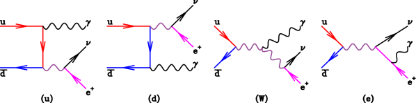
Figure 1: Topologies of diagrams included at lowest order, shown for the specific case of $u\bar{d}\to\gamma\nu_{e}e^{+}$. Note that diagrams (u) and (d) are proportional to $Q_{u}$ and $Q_{d}$ respectively, whereas diagrams, (W) and (e) are proportional to $Q_{u}-Q_{d}$.

The lowest-order graphs are shown in Fig. 1. We separate the sub-amplitudes into contributions that are sensitive to individual electric charges,

$$A^{(0)}(5_{\gamma}^{h_{5}}) = \left(Q_{u}\,A^{u}_{\mathrm{tree}}(5_{\gamma}^{h_{5}})+Q_{d}\,A^{d}_{\mathrm{tree}}(5_{\gamma}^{h_{5}})\right)P(s_{34})$$

$$+(Q_{u}-Q_{d})\,\left(A^{e}_{\mathrm{tree}}(5_{\gamma}^{h_{5}})+A^{W}_{\mathrm{tree}}(5_{\gamma}^{h_{5}})P(s_{34})\right)P(s_{345})\,,$$

where we have also pulled out factors of the $W$-boson propagator defined by,

$$P(s)=\frac{1}{s-m_{W}^{2}}=\frac{1}{s-M_{W}^{2}+iM_{W}\Gamma_{W}},$$ (3)

and $m_{W}^{2}=M_{W}^{2}-iM_{W}\Gamma_{W}$ indicates that we are working in the complex-mass scheme. These sub-amplitudes are clearly not individually gauge invariant in the electroweak sector.

2.1.2 Tree-level amplitudes

The components of the tree-level Born amplitude are,

$$A^{u}_{\mathrm{tree}}(5_{\gamma}^{-}) = 0,\;\;\;A^{d}_{\mathrm{tree}}(5_{\gamma}^{-})=\frac{\left[14\right]^{2}\left\langle 43\right\rangle}{\left[15\right]\left[25\right]},\;\;\;A^{W}_{\mathrm{tree}}(5_{\gamma}^{-})=\frac{\left[14\right]^{2}\left\langle 43\right\rangle\left\langle 25\right\rangle}{\left[15\right]},$$

$$A^{e}_{\mathrm{tree}}(5_{\gamma}^{-}) = \frac{\left[14\right]^{2}\left\langle 32\right\rangle}{\left[15\right]\left[45\right]},$$ (4)

$$A^{u}_{\mathrm{tree}}(5_{\gamma}^{+}) = \frac{\left\langle 23\right\rangle^{2}\left[34\right]}{\left\langle 15\right\rangle\left\langle 25\right\rangle},\;\;\;A^{d}_{\mathrm{tree}}(5_{\gamma}^{+})=0,\;\;\;A^{W}_{\mathrm{tree}}(5_{\gamma}^{+})=\frac{\left\langle 23\right\rangle^{2}\left[43\right]\left[15\right]}{\left\langle 25\right\rangle},$$

$$A^{e}_{\mathrm{tree}}(5_{\gamma}^{+}) = \frac{\left\langle 23\right\rangle^{2}\left[31\right]}{\left\langle 25\right\rangle\left\langle 45\right\rangle}.$$ (5)

For all of the sub-amplitudes except for the one in which the photon is radiated from the positron in the $W$-boson decay, $A^{e}$, there is a simple rule for flipping the helicities of the photon,

$$A^{u}_{\mathrm{tree}}(1_{\bar{u}}^{+},2_{d}^{-},3_{\nu}^{-},4_{{e}}^{+},5_{\gamma}^{-h_{5}}) = A^{d}_{\mathrm{tree}}(2_{\bar{u}}^{+},1_{d}^{-},4_{\nu}^{-},3_{{e}}^{+},5_{\gamma}^{h_{5}})\,\bigl{\{}\langle\rangle\leftrightarrow[]\bigr{\}}\,,$$ (6)

$$A^{W}_{\mathrm{tree}}(1_{\bar{u}}^{+},2_{d}^{-},3_{\nu}^{-},4_{{e}}^{+},5_{\gamma}^{-h_{5}}) = -A^{W}_{\mathrm{tree}}(2_{\bar{u}}^{+},1_{d}^{-},4_{\nu}^{-},3_{{e}}^{+},5_{\gamma}^{h_{5}})\,\bigl{\{}\langle\rangle\leftrightarrow[]\bigr{\}}\,.$$ (7)

Complete amplitudes for the charge-conjugate process,

$$0\rightarrow u(p_{1})+\bar{d}(p_{2})+e^{-}(p_{3})+\bar{\nu}_{e}(p_{4})+\gamma(p_{5})$$ (8)

are given by a transformation on the entire amplitude similar to the one given above for flipping helicities,

$$\mathcal{A}^{(0)}(1^{+}_{u},2^{-}_{\bar{d}},3^{-}_{{e}},4^{+}_{\nu},5^{-h_{5}}_{\gamma})=\mathcal{A}^{(0)}(2^{+}_{\bar{u}},1^{-}_{d},4^{-}_{\nu},3^{+}_{{e}},5^{h_{5}}_{\gamma})\,\bigl{\{}\langle\rangle\leftrightarrow[]\bigr{\}}\,.$$ (9)

2.1.3 One-loop amplitude

Five-parton results at one loop are taken from Ref. Dixon:1998py and supplemented with the contributions from radiation in decay. They could equivalently be taken from Ref. Gehrmann:2011ab and we have checked explicitly that the two forms are identical numerically.

2.1.4 Two-loop amplitude

Genuine two-loop contributions for Drell-Yan type processes were pioneered in Ref. Matsuura:1988sm . The $W\gamma$ results that we use in our calculation are taken from Ref. Gehrmann:2011ab , where the two-loop amplitude after UV renormalization at $\mu^{2}=s_{34}$, is presented as the finite term remaining after extraction of the predicted IR singularity structure at two loops Catani:1998bh :

$$\Omega = \Omega^{(0)}+\left(\frac{\alpha_{s}(\mu^{2})}{2\pi}\right)\Omega^{(1)}+\left(\frac{\alpha_{s}(\mu^{2})}{2\pi}\right)^{2}\Omega^{(2)}+O(\alpha_{s}^{3})$$ (10)

$$= \Omega^{(0)}+\left(\frac{\alpha_{s}(\mu^{2})}{2\pi}\right)(\Omega^{(1),f}+\Omega^{(0)}\boldsymbol{I}_{1}(\epsilon))$$

$$+\left(\frac{\alpha_{s}(\mu^{2})}{2\pi}\right)^{2}(\Omega^{(2),f}+\Omega^{(1),f}\boldsymbol{I}_{1}(\epsilon)+\Omega^{(0)}(\boldsymbol{I}_{1}(\epsilon)^{2}+\boldsymbol{I}_{2}(\epsilon)))\,.$$

The finite parts $\Omega^{(1),f},\Omega^{(2),f}$ differ by finite terms from the hard function, $H$. The construction of the hard function from the results for the one- and two-loop amplitude is spelled out in refs. Becher:2013vva ; Campbell:2016yrh ,

$$H = H^{(0)}+\frac{\alpha_{s}(\mu^{2})}{2\pi}H^{(1)}+\left(\frac{\alpha_{s}(\mu^{2})}{2\pi}\right)^{2}H^{(2)}\,,$$ (11)

$$H^{(0)} = \Omega^{(0)}\,,$$

$$H^{(1)} = \Omega^{(1),f}+\boldsymbol{J}^{(1)}\Omega^{(0)}\,,$$

$$H^{(2)} = \Omega^{(2),f}+\boldsymbol{J}^{(1)}\Omega^{(1),\text{f}}+\boldsymbol{J}^{(2)}\Omega^{(0)}\,,$$ (12)

where the $\boldsymbol{J}$ are finite functions formed by combining the perturbative expansion of the Catani singularity structure and the perturbative expansion of the inverse of the $\boldsymbol{Z}$ matrix,

$$\boldsymbol{Z}^{-1}=1+\boldsymbol{Z}^{(1)}(\epsilon)\frac{\alpha_{s}(\mu^{2})}{2\pi}+\boldsymbol{Z}^{(2)}(\epsilon)\left(\frac{\alpha_{s}(\mu^{2})}{2\pi}\right)^{2}+\ldots$$ (13)

Explicitly,

$$\boldsymbol{J}^{(1)}=\boldsymbol{I}^{(1)}(\epsilon)+\boldsymbol{Z}^{(1)}(\epsilon),\;\;\;\boldsymbol{J}^{(2)}=\boldsymbol{I}^{(2)}(\epsilon)+\left(\boldsymbol{I}^{(1)}(\epsilon)+\boldsymbol{Z}^{(1)}(\epsilon)\right)\boldsymbol{I}^{(1)}(\epsilon)+\boldsymbol{Z}^{(2)}(\epsilon)\,,$$ (14)

resulting in,

$$\boldsymbol{J}^{(1)} = -\frac{C_{F}}{2}(L^{2}+3L-\zeta_{2})\,,$$ (15)

$$\boldsymbol{J}^{(2)} = \frac{C_{F}^{2}}{32}[4L^{4}+24L^{3}+36L^{2}-8\zeta_{2}L^{2}-24\zeta_{2}L+10\zeta_{4}]$$

$$+\frac{C_{F}T_{R}n_{f}}{18}[2L^{3}+19L^{2}+30L+3\zeta_{2}L+2\zeta_{2}+3\zeta_{3}]$$

$$-\frac{C_{F}C_{A}}{144}[44L^{3}+466L^{2}-72\zeta_{2}L^{2}+804L-150\zeta_{2}L+32\zeta_{2}+66\zeta_{3}+45\zeta_{4}],$$

where $n_{f}$ is the number of active flavours and

$$C_{F}=\frac{4}{3},\;\;N=3,\;\;T_{R}=\frac{1}{2},\;\;\zeta_{2}=\frac{\pi^{2}}{6},\;\;\zeta_{3}\approx 1.20206,\;\;\zeta_{4}=\frac{\pi^{4}}{90},\;\;L=\ln\frac{\mu^{2}}{-s_{12}-i0}\,.$$ (17)

2.2 6-parton amplitude

2.2.1 Structure of the 6-parton amplitude

We calculate the one-loop helicity amplitudes for,

$$0\rightarrow\bar{u}(p_{1})+d(p_{2})+\nu_{e}(p_{3})+e^{+}(p_{4})+\gamma(p_{5})+g(p_{6})\,.$$ (18)

Our calculation includes contributions where the photon is radiated of the positron. The reduced amplitude, $A^{(0)}$, is defined as,

$$\mathcal{A}^{(0)}(1^{+}_{\bar{u}},2^{-}_{d},3^{-}_{\nu},4^{+}_{{e}},5^{h_{5}}_{\gamma},6^{h_{6}}_{g}) = i\sqrt{2}\,eg_{W}^{2}g_{s}\,t^{a_{6}}_{i_{2}i_{1}}\cdot A^{(0)}(5^{h_{5}}_{\gamma},6^{h_{6}}_{g})\,,$$ (19)

with $\mathop{\rm tr}\nolimits(t^{a}t^{b})=\delta^{ab}$. Furthermore, it is useful to further separate the sub-amplitudes into contributions that are sensitive to individual electric charges,

$$A^{(0)}(5_{\gamma}^{h_{5}},6_{g}^{h_{6}}) = \left(Q_{u}\,A^{u}_{\mathrm{tree}}(5_{\gamma}^{h_{5}},6_{g}^{h_{6}})+Q_{d}\,A^{d}_{\mathrm{tree}}(5_{\gamma}^{h_{5}},6_{g}^{h_{6}})\right)P(s_{34})$$

$$+(Q_{u}-Q_{d})\,\left(A^{e}_{\mathrm{tree}}(5_{\gamma}^{h_{5}},6_{g}^{h_{6}})+A^{W}_{\mathrm{tree}}(5_{\gamma}^{h_{5}},6_{g}^{h_{6}})P(s_{34})\right)P(s_{345})\,.$$

2.2.2 Tree-level amplitudes

The components of the tree-level amplitude for a photon and a gluon both of positive helicity are,

$$A^{u}_{\mathrm{tree}}(5_{\gamma}^{+},6_{g}^{+}) = \frac{\left\langle 12\right\rangle\left\langle 23\right\rangle^{2}\left[43\right]}{\left\langle 15\right\rangle\left\langle 16\right\rangle\left\langle 25\right\rangle\left\langle 26\right\rangle}\,,$$ (21)

$$A^{d}_{\mathrm{tree}}(5_{\gamma}^{+},6_{g}^{+}) = 0\,,$$ (22)

$$A^{e}_{\mathrm{tree}}(5_{\gamma}^{+},6_{g}^{+}) = \frac{\left\langle 23\right\rangle^{2}\langle 2|(4+5)|3]}{\left\langle 16\right\rangle\left\langle 25\right\rangle\left\langle 26\right\rangle\left\langle 45\right\rangle}\,,$$ (23)

$$A^{W}_{\mathrm{tree}}(5_{\gamma}^{+},6_{g}^{+}) = \frac{\left\langle 23\right\rangle^{2}\left[43\right]\langle 2|(1+6)|5]}{\left\langle 16\right\rangle\left\langle 25\right\rangle\left\langle 26\right\rangle}\,.$$ (24)

For the case where the photon has negative helicity and the gluon positive helicity we have,

$$A^{u}_{\mathrm{tree}}(5_{\gamma}^{-},6_{g}^{+}) = -\frac{\left\langle 23\right\rangle\left[16\right]\langle 5|(2+3)|4])}{\left[15\right]\left\langle 16\right\rangle s_{234}}\,,$$ (25)

$$A^{d}_{\mathrm{tree}}(5_{\gamma}^{-},6_{g}^{+}) = -\Big{[}\frac{\langle 2|(1+6)|4]\langle 3|(2+5)|1]}{\left[15\right]\left\langle 16\right\rangle\left[25\right]\left\langle 26\right\rangle}+\frac{\left[14\right]\left\langle 25\right\rangle\langle 3|(1+4)|6]}{\left[25\right]\left\langle 26\right\rangle s_{134}}\Big{]}\,,$$ (26)

$$A^{e}_{\mathrm{tree}}(5_{\gamma}^{-},6_{g}^{+}) = -\frac{\left[14\right]\langle 2|(1+6)|4]\left\langle 23\right\rangle}{\left\langle 16\right\rangle\left\langle 26\right\rangle\left[15\right]\left[45\right]}\,,$$ (27)

$$A^{W}_{\mathrm{tree}}(5_{\gamma}^{-},6_{g}^{+}) = -\frac{\langle 2|(1+6)|4](\left\langle 25\right\rangle\left\langle 34\right\rangle\left[14\right]+\left\langle 26\right\rangle\left\langle 35\right\rangle\left[16\right])}{\left\langle 16\right\rangle\left\langle 26\right\rangle\left[15\right]}\,.$$ (28)

For all of the sub-amplitudes except for the one in which the photon is radiated from the positron in the $W$-boson decay, $A^{e}$, there is a simple rule for flipping the helicities of the photon and gluon,

$$A^{u}_{\mathrm{tree}}(1_{\bar{u}}^{+},2_{d}^{-},3_{\nu}^{-},4_{{e}}^{+},5_{\gamma}^{-h_{5}},6_{g}^{-h_{6}}) = A^{d}_{\mathrm{tree}}(2_{\bar{u}}^{+},1_{d}^{-},4_{\nu}^{-},3_{{e}}^{+},5_{\gamma}^{h_{5}},6_{g}^{h_{6}})\,\bigl{\{}\langle\rangle\leftrightarrow[]\bigr{\}}\,,$$ (29)

$$A^{W}_{\mathrm{tree}}(1_{\bar{u}}^{+},2_{d}^{-},3_{\nu}^{-},4_{{e}}^{+},5_{\gamma}^{-h_{5}},6_{g}^{-h_{6}}) = -A^{W}_{\mathrm{tree}}(2_{\bar{u}}^{+},1_{d}^{-},4_{\nu}^{-},3_{{e}}^{+},5_{\gamma}^{h_{5}},6_{g}^{h_{6}})\,\bigl{\{}\langle\rangle\leftrightarrow[]\bigr{\}}\,.$$ (30)

For the remaining amplitudes we have,

$$A^{e}_{\mathrm{tree}}(5_{\gamma}^{-},6_{g}^{-}) = \frac{\left[14\right]^{2}\langle 3|4+5|1]}{\left[26\right]\left[15\right]\left[16\right]\left[45\right]}\,,$$ (31)

and,

$$A^{e}_{\mathrm{tree}}(5_{\gamma}^{+},6_{g}^{-}) = -\frac{\langle 2|(4+5)|1]\langle 3|(2+6)|1]}{\left[26\right]\left[16\right]\left\langle 25\right\rangle\left\langle 45\right\rangle}\,.$$ (32)

Complete amplitudes for the charge-conjugate process,

$$0\rightarrow u(p_{1})+\bar{d}(p_{2})+e^{-}(p_{3})+\bar{\nu}_{e}(p_{4})+\gamma(p_{5})+g(p_{6})$$ (33)

are given by a transformation on the entire amplitude similar to the one given above for flipping helicities,

$$\mathcal{A}^{(0)}(1^{+}_{u},2^{-}_{\bar{d}},3^{-}_{{e}},4^{+}_{\nu},5^{-h_{5}}_{\gamma},6^{-h_{6}}_{g})=\mathcal{A}^{(0)}(2^{+}_{\bar{u}},1^{-}_{d},4^{-}_{\nu},3^{+}_{{e}},5^{h_{5}}_{\gamma},6^{h_{6}}_{g})\,\bigl{\{}\langle\rangle\leftrightarrow[]\bigr{\}}\,.$$ (34)

The $W$-boson component of this amplitude can be isolated by partial fractioning

$$P(s_{34})P(s_{345})=\frac{1}{s_{345}-s_{34}}\,\Big{[}P(s_{34})-P(s_{345})\Big{]}$$ (35)

and dropping all terms not containing $P(s_{34})$. The result in this limit is given in Ref. Dixon:1998py .

2.2.3 One-loop amplitude

We extract a similar factor at the one-loop level,

$$\mathcal{A}^{(1)}(5^{h_{5}}_{\gamma},6_{g}^{h_{6}})=\quad i\sqrt{2}\,eg_{W}^{2}g_{s}^{3}\,c_{\Gamma}\;t^{a_{6}}_{i_{2}i_{1}}\bigg{\{}N_{c}\,A^{(1)}_{\mathrm{lc}}(5^{h_{5}}_{\gamma},6^{h_{6}}_{g})+\frac{1}{N_{c}}\,A^{(1)}_{\mathrm{sl}}(5_{\gamma}^{h_{5}},6_{g}^{h_{6}})\bigg{\}}\,,$$ (36)

where this time, in addition, we have performed a decomposition into leading- (‘$\mathrm{lc}$’) and subleading-colour (‘$\mathrm{sl}$’) components. We work in dimensional regularization with $d=4-2\epsilon$, resulting in the overall factor $c_{\Gamma}$ given by,

$$c_{\Gamma}=\frac{1}{(4\pi)^{2-\epsilon}}\frac{\Gamma(1+\epsilon)\Gamma^{2}(1-\epsilon)}{\Gamma(1-2\epsilon)}=\frac{1}{(4\pi)^{2-\epsilon}}\frac{1}{\Gamma(1-\epsilon)}+O(\epsilon^{3})\,.$$ (37)

Furthermore, it is useful to further separate the sub-amplitudes into contributions that are sensitive to individual electric charges,

$$A^{(1)}_{\mathrm{lc}}(5_{\gamma}^{h_{5}},6_{g}^{h_{6}}) = \left(Q_{u}\,A^{u}_{\mathrm{lc}}(5_{\gamma}^{h_{5}},6_{g}^{h_{6}})+Q_{d}\,A^{d}_{\mathrm{lc}}(5_{\gamma}^{h_{5}},6_{g}^{h_{6}})\right)P(s_{34})$$

$$+(Q_{u}-Q_{d})\,\left(A^{e}_{\mathrm{lc}}(5_{\gamma}^{h_{5}},6_{g}^{h_{6}})+A^{W}_{\mathrm{lc}}(5_{\gamma}^{h_{5}},6_{g}^{h_{6}})P(s_{34})\right)P(s_{345})\,,$$

(and similarly for $A^{(1)}_{\mathrm{sl}}$). Note that the individual terms in this separation are not invariant under electroweak or QCD gauge transformations. Full analytic results for $A_{\mathrm{lc}}$ and $A_{\mathrm{sl}}$ are given in Appendix C. We have checked numerically that our results agree perfectly with those provided by OpenLoops Cascioli:2011va , but are faster by at least a factor of four.

2.3 7-parton amplitude

2.3.1 Two-quark two-gluon processes

We can decompose the amplitude for the two-gluon process $0\rightarrow\bar{u}(p_{1})+d(p_{2})+\nu_{e}(p_{3})+e^{+}(p_{4})+\gamma(p_{5})+g(p_{6})+g(p_{7})$ into two colour-ordered sub-amplitudes,

$$\mathcal{A}^{(0)}(1^{+}_{\bar{u}},2^{-}_{d},3^{-}_{\nu},4^{+}_{{e}},5^{h_{5}}_{\gamma},6^{h_{6}}_{g},7^{h_{7}}_{g})=i\,\sqrt{2}\,eg_{W}^{2}g_{s}^{2}$$ (39)

$$\times \,\left[\left(t^{a_{6}}t^{a_{7}}\right)_{i_{2}i_{1}}\cdot A^{67}(5^{h_{5}}_{\gamma},6^{h_{6}}_{g},7^{h_{7}}_{g})+\left(t^{a_{7}}t^{a_{6}}\right)_{i_{2}i_{1}}\cdot A^{76}(5^{h_{5}}_{\gamma},6^{h_{6}}_{g},7^{h_{7}}_{g})\right]\,.$$

Full analytic results for the colour-ordered trees are presented in subsection (D.1). Squaring the amplitude and summing over the colours of the gluons, we obtain,

$$\sum_{a_{6},a_{7}}\sum_{h_{5},h_{6},h_{7}}\big{|}\mathcal{A}^{(0)}(1^{+}_{\bar{u}},2^{-}_{d},3^{-}_{\nu},4^{+}_{{e}},5^{h_{5}}_{\gamma},6^{h_{6}}_{g},7^{h_{7}}_{g})\big{|}^{2}=2e^{2}g_{W}^{4}g_{s}^{4}(N^{2}-1)$$ (40)

$$\times \sum_{h_{5},h_{6},h_{7}}\Big{[}N\left(\big{|}A^{67}(5^{h_{5}}_{\gamma},6^{h_{6}}_{g},7^{h_{7}}_{g})\big{|}^{2}+\big{|}A^{76}(5^{h_{5}}_{\gamma},6^{h_{6}}_{g},7^{h_{7}}_{g})\big{|}^{2}\right)$$

$$- \frac{1}{N}\big{|}A^{67}(5^{h_{5}}_{\gamma},6^{h_{6}}_{g},7^{h_{7}}_{g})+A^{76}(5^{h_{5}}_{\gamma},6^{h_{6}}_{g},7^{h_{7}}_{g})\big{|}^{2}\Big{]}\,.$$

2.3.2 Four-quark processes

In a similar fashion the amplitude for the process, $0\rightarrow\bar{u}(p_{1})+d(p_{2})+\nu_{e}(p_{3})+e^{+}(p_{4})+\gamma(p_{5})+q(p_{6})+\bar{q}(p_{7})$ for the simple case of $q$ and $\bar{q}$ consisting of non-identical flavours can be written as,

$$\mathcal{A}^{(0)}(1^{+}_{\bar{u}},2^{-}_{d},3^{-}_{\nu},4^{+}_{{e}},5^{h_{5}}_{\gamma},6^{h_{6}}_{q},7^{h_{7}}_{\bar{q}})=i\,\sqrt{2}\,eg_{W}^{2}g_{s}^{2}\,\sum_{a}t^{a}_{i_{7}i_{1}}\,t^{a}_{i_{8},i_{2}}\,\mathcal{A}^{(0)}(5^{h_{5}}_{\gamma},6^{h_{6}}_{q},7^{h_{7}}_{\bar{q}})\,.$$ (41)

Many other needed amplitudes are related to the amplitude in Eq. (41) by crossing. Full analytic results are presented in subsection (D.2). Performing the colour sums, the squared amplitude is written as,

$$\sum_{h_{5}}\Big{|}\mathcal{A}^{(0)}(1^{+}_{\bar{u}},2^{-}_{d},3^{-}_{\nu},4^{+}_{{e}},5^{h_{5}}_{\gamma},6^{+}_{q},7^{-}_{\bar{q}})\Big{|}^{2}=2e^{2}g_{W}^{4}g_{s}^{4}(N^{2}-1)\sum_{h_{5}}\Big{|}\mathcal{A}^{(0)}(5^{h_{5}}_{\gamma},6^{+}_{q},7^{-}_{\bar{q}})\Big{|}^{2}\,.$$ (42)

The case for identical quarks is slightly more complicated, but can be easily derived from the results presented.

3 $N$-jettiness method for NNLO cross sections

3.1 Jettiness

A collision of partons $a$ and $b$ with momentum fractions $x_{a,b}$, originating from the incoming-beam protons with momenta $p_{a,b}$, can potentially produce a final state including $N$ jets with momenta $\{p_{i}\}$. The jettiness of parton $j$ with momentum $q_{j}$ is defined as

$${\cal T}_{N}(q_{j})=\min_{i=a,b,1,\ldots,N}\left\{\frac{2\,p_{i}\cdot q_{j}}{{P_{i}}}\right\}\ .$$ (43)

We denote by $E_{i}$ the jet or beam energy. $P_{i}$ is a measure of the jet/beam hardness. In our numerical results we set this equal to twice the jet/beam energy, $P_{i}=2E_{i}$ Stewart:2010tn . We can now define the event jettiness, or $N$-jettiness, as the sum over all the $M$ final-state parton-jettiness values

$${\cal T}_{N}=\sum_{j=1}^{M}{\cal T}_{N}(q_{j})=\sum_{j=1}^{M}\min_{i=a,b,1,\ldots,N}\left\{\frac{2\,p_{i}\cdot q_{j}}{{P_{i}}}\right\}\ .$$ (44)

For Leading Order (LO) events we have $\{q_{i}\}=\{p_{i}\}$ and the event jettiness is zero. Beyond LO extra particles are emitted ($M>N$), the event jettiness goes to zero only in the soft/collinear limit. The event $N$-jettiness can be used in a non-local subtraction approach where we can isolate the doubly unresolved region of the phase space by demanding ${\cal T}_{N}<{\cal T}_{N}^{cut}$ Boughezal:2011jf ; Gaunt:2015pea .

3.2 Colour singlet final states

For the case at hand we have no coloured final-state partons at leading order. We can therefore use the event shape variable ${\cal T}_{0}$ to regulate the initial-state radiation. By demanding ${\cal T}_{0}<{\cal T}_{0}^{cut}$ one isolates the doubly unresolved regions of phase space. In this region the jettiness has simple factorization properties derivable using soft-collinear effective theory. We exploit the fact that the matrix elements in the soft/collinear approximation can be analytically integrated over this region and added to the virtual contributions. The regions of phase space where ${\cal T}_{0}>{\cal T}_{0}^{cut}$ are integrated over numerically.

In the context of MCFM, the application of the $N$-jettiness method to the particular case of processes involving the production of a colour-singlet final state at the Born level has been described in a series of papers Boughezal:2016wmq ; Campbell:2016yrh ; Campbell:2017aul . In particular refs. Boughezal:2016wmq ; Campbell:2017aul contain details of the construction of the soft function and of the modifications to the two-loop matrix elements needed to construct the hard function.

For the process studied in this paper the cut that defines the below-cut and above-cut contributions is expressed in terms of a dimensionless variable $\epsilon$ that is defined by,

$${\cal T}_{0}^{cut}=\epsilon\times m_{\ell\nu\gamma}\,,$$ (45)

where $m_{\ell\nu\gamma}^{2}=(p_{\ell}+p_{\nu}+p_{\gamma})^{2}$. Compared to a fixed (dimensionful) value of the cut this yields better numerical stability and aids an automatic fitting of the ${\cal T}_{0}^{cut}$ dependence that can be used to extrapolate the ${\cal T}_{0}^{cut}\to 0$ result.

4 Setup of numerical results for $W(\to e\nu)+\gamma$ cross section

4.1 Parameter setup

We investigate the processes $pp\to e^{-}\bar{\nu}_{e}\gamma$ and $pp\to e^{+}\nu_{e}\gamma$, using the parameters shown in Table 2. The parton distributions sets used are the sets, ’NNPDF30_xx_as_0118’ with xx=lo,nlo,nnlo according to the order calculated Buckley:2014ana . In all three cases the value of the strong coupling is taken to be $\alpha_{s}(M_{z})=0.118$. The electromagnetic coupling $\alpha$ is a derived parameter, calculated with the definition shown in Table 2. The complex-mass scheme is used, so that the Weinberg angle is also complex. In this section our parameter choices are made so as to agree with the choices made in Ref. Grazzini:2017mhc .

$M_{W}$	80.385 GeV	$\Gamma_{W}$	2.0854 GeV
$M_{Z}$	91.1876 GeV	$\Gamma_{Z}$	2.4952 GeV
$G_{\mu}$	$1.166390\times 10^{-5}$ GeV-2
$m_{W}^{2}=M_{W}^{2}-iM_{W}\Gamma_{W}$	$(6461.748225-167.634879\,i)$ GeV2
$m_{Z}^{2}=M_{Z}^{2}-iM_{Z}\Gamma_{Z}$	$(8315.17839376-227.53129952\,i)$ GeV2
$\cos^{2}\theta_{W}={m_{W}^{2}}/{m_{Z}^{2}}$	$(0.7770725897054007+0.001103218322282256\,i)$
$\alpha=\frac{\sqrt{2}G_{\mu}}{\pi}M_{W}^{2}(1-\frac{M_{W}^{2}}{M_{Z}^{2}})$	$7.56246890198475\times 10^{-3}$ giving $1/\alpha\approx 132.23\ldots$

Table 2: Input and derived parameters used for our numerical estimates.

We construct an explicitly unitary, CP-conserving CKM matrix in the standard form Zyla:2020zbs with $(c_{ij}=\cos\theta_{ij},s_{ij}=\sin\theta_{ij}$)

$$V_{CKM}=\left(\begin{matrix}c_{12}c_{13}&c_{13}s_{12}&s_{13}\\ -c_{23}s_{12}-c_{12}s_{13}s_{23}&c_{12}c_{23}-s_{12}s_{13}s_{23}&c_{13}s_{23}\\ s_{12}s_{23}-c_{12}c_{23}s_{13}&-c_{12}s_{23}-c_{23}s_{12}s_{13}&c_{13}c_{23}\end{matrix}\right)\,.$$ (46)

Starting with the following values for four of the measurements $V_{ud}=0.97417$, $V_{us}=0.22480$, $V_{ub}=0.00409$, $V_{cb}=0.04050$, and the following definitions for the angles

$$s_{12} = \frac{V_{us}}{\sqrt{V_{ud}^{2}+V_{us}^{2}}},\;\;\;s_{23}=\frac{V_{cb}}{V_{us}}{s_{12}},\;\;\;s_{13}=V_{ub}\,,$$ (47)

we obtain a unitary CKM matrix of the following form,

$$V_{CKM}=\left(\begin{matrix}0.97438&0.22485&0.00409\\ -0.22483&0.97356&0.04051\\ 0.00513&-0.04039&0.99917\end{matrix}\right)\,.$$ (48)

The third row in Eq. (48) involving couplings to the top is irrelevant for the current calculation.

We estimate the scale variation by varying the renormalization $(\mu_{R}=\kappa_{R}\mu_{0})$ and factorization $(\mu_{F}=\kappa_{F}\mu_{0})$ scales independently by a factor $\kappa_{R,F}$ about the central scale $\mu_{0}$,

$$\mu_{0}=\sqrt{M_{W}^{2}+(p_{T}^{\gamma})^{2}}.$$ (49)

We choose $\kappa_{R,F}=\frac{1}{2}$ or $2$. This gives us eight possible scale variations about the central scale $(1,1)$, or six variations if we drop the choices where $\kappa_{F}$ and $\kappa_{R}$ differ by a factor of 4,

$$\text{7-point}:(\kappa_{R},\kappa_{F}) = (1,1),(\frac{1}{2},1),(1,\frac{1}{2}),(2,1),(1,2),(\frac{1}{2},\frac{1}{2}),(2,2)\,;$$

$$\text{9-point}:(\kappa_{R},\kappa_{F}) = (1,1),(\frac{1}{2},1),(1,\frac{1}{2}),(2,1),(1,2),(\frac{1}{2},\frac{1}{2}),(2,2),(\frac{1}{2},2),(2,\frac{1}{2})\,.$$ (50)

The assigned error is the maximum of the deviation from the value at the central scale $(1,1)$ in both the up and down directions. We note that although the 7-point variation has become a somewhat standard procedure, the extension to the 9-point variation for our process is motivated by an accidental cancellation between renormalization and factorization scale dependence observed at NLO Campbell:2011bn .

4.2 Photon isolation

Rather than performing a calculation that implements the effects of photon fragmentation, necessitating the use of data-derived fragmentation functions, we pursue a simpler approach that is readily applied in the NNLO case. We use a “smooth cone” isolation procedure Frixione:1998jh to avoid infrared singularities arising from the emission of photons from partons. In this method one defines a cone of radius $R=\sqrt{(\Delta\eta)^{2}+(\Delta\phi)^{2}}$ around the photon, where $\Delta\eta$ and $\Delta\phi$ are the pseudorapidity and azimuthal angle difference between the photon and any parton. The total partonic transverse energy inside a cone with radius $R$ is then constrained according to,

$$E_{T}^{had}(R)<\epsilon_{s}\,E_{T}^{\gamma}\left(\frac{1-\cos R}{1-\cos R_{s}}\right)^{n}\,,$$ (51)

for all cones $R<R_{s}$, where $E_{T}^{\gamma}$ is the transverse photon energy, and $\epsilon_{s}$, $R_{s}$ and $n$ are parameters.

In addition, one can also choose to further impose an additional fixed-cone isolation that more closely mimics the experimental sensitivity to photon isolation effects, resulting in a so-called “hybrid isolation” scheme Siegert:2016bre ; Chen:2019zmr . The form of this additional cut is,

$$E_{T}^{had}(R)<\epsilon_{f}\,E_{T}^{\gamma}+E_{T}^{f}\qquad\mbox{for~{}}R<R_{f}\,.$$ (52)

We shall make use of an additional cut of this form in Section 6.

4.3 A first look at results at $\sqrt{s}=13$ TeV

We first perform a comparison with the MATRIX results given in Ref. Grazzini:2017mhc , that are computed at $\sqrt{s}=13$ TeV and using the cuts shown in Table 3.

Electron cuts	$p_{T,e}>25$ GeV, $|\eta_{e}|<2.47$
Neutrino cuts	$p_{T}^{\rm missing}>35$ GeV
Photon cuts	$p_{T,\gamma}>15$ GeV, $|\eta_{\gamma}|<2.47$
Separation cuts	$\Delta_{ej}>0.3,\Delta_{\gamma j}>0.3,\Delta_{e\gamma}>0.7$
Photon Isolation	Isolation with $n=1$, $\epsilon_{s}=0.5$, $R_{s}=0.4$, c.f. Eq. (51)
Jet definition	Anti-$k_{T}$ algorithm with R=0.4, $p_{T,j}>30$ GeV, $|\eta_{j}|<4.4$

Table 3: Cuts used for the cross-section results in section 4.3.

The results of the MCFM calculation in this setup are shown in Table 4, indicating the cross sections obtained at each order of perturbation theory up to NNLO, both with and without the effects of the CKM matrix. We have run the NNLO calculation to ensure that the Monte Carlo uncertainty on the result at $\epsilon=10^{-4}$, as defined in Eq. (45), is at the 2 per-mille level. An automated fit to the $\tau$ dependence is performed using the known form of the residual power-corrections to the SCET factorization formula Campbell:2019dru ,

$$\sigma=\sigma_{0}+a\epsilon\log^{3}\epsilon+b\epsilon\log^{2}\epsilon\,.$$ (53)

The result (with the CKM matrix included) is illustrated in Fig. 2, yielding a correction to the $\epsilon=10^{-4}$ result of around 1%, with a corresponding uncertainty of about 3 per-mille. The difference between the result using a diagonal CKM matrix, and the result with the CKM matrix of Eq. (48) included, is about $0.8\%$ at LO but decreases to about $0.3\%$ at NLO and NNLO. Note that because of the unitarity of the CKM matrix, parton processes involving $gq$ or $g\bar{q}$ are approximately unchanged by including a non-diagonal CKM matrix. At NLO $gq$ and $g\bar{q}$ initial states contribute $39\%$ of the cross section, which explains the reduced effect of a non-diagonal CKM matrix.

Our results with a diagonal CKM matrix are in perfect agreement within mutual uncertainties with those from MATRIX (reported in Table 6 of Ref. Grazzini:2017mhc ) which are,

$$\sigma^{\rm extrap}_{{\rm MATRIX}}(pp\to e^{+}\nu_{e}\gamma) = 2671(35)^{+3.8\%}_{-3.6\%}\,{\rm fb},$$ (54)

$$\sigma^{\rm extrap}_{{\rm MATRIX}}(pp\to e^{-}\bar{\nu}_{e}\gamma) = 2256(15)^{+3.7\%}_{-3.5\%}\,{\rm fb}.$$ (55)

We note that the uncertainty in the result, stemming from the fit (or, equivalently, the extrapolation performed in MATRIX) is smaller in our case.

Process	$\sigma_{\text{LO}}$ [fb]	$\sigma_{\text{NLO}}$ [fb]	$\sigma_{\text{NNLO}}^{\epsilon=10^{-4}}$ [fb]	$\sigma_{\text{NNLO}}^{\rm fit}$ [fb]
$pp\to e^{+}\nu_{e}\gamma$ (no CKM)	861.6	$2187^{+6.6\%}_{-5.3\%}$	2689(5)	$2668(8)^{+3.9\%}_{-3.7\%}$
$pp\to e^{+}\nu_{e}\gamma$ (with CKM)	854.6	$2181^{+6.6\%}_{-5.3\%}$	2681(5)	$2661(8)^{+3.9\%}_{-3.7\%}$
$pp\to e^{-}\bar{\nu}_{e}\gamma$ (no CKM)	726.2	$1849^{+6.6\%}_{-5.3\%}$	2260(4)	$2240(7)^{+3.7\%}_{-3.5\%}$
$pp\to e^{-}\bar{\nu}_{e}\gamma$ (with CKM)	720.1	$1843^{+6.6\%}_{-5.3\%}$	2252(4)	$2228(7)^{+3.7\%}_{-3.5\%}$

Table 4: Cross-section results with the cuts of Table 3. The theoretical error is estimated by a 7-point scale variation. Parentheses indicate the residual error resulting from numerical integration of the NNLO result (this error is beyond the indicated number of digits at NLO).

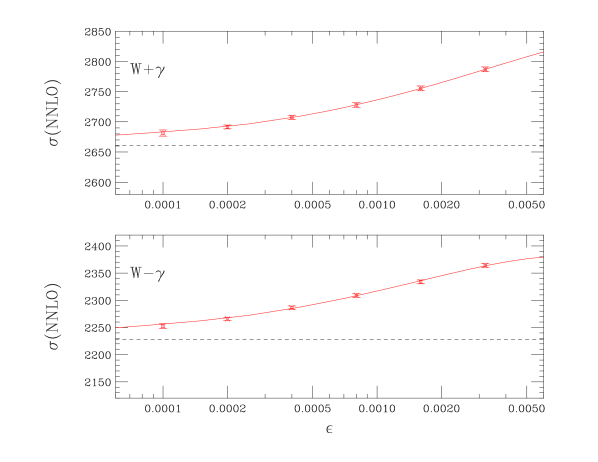
Figure 2: $\tau$-cut dependence of the NNLO cross sections for $W^{+}\gamma$ (upper) and $W^{-}\gamma$ (lower) production using our setup. The solid lines indicate the results of a fit to the points using the expected form of power corrections given in Eq. (53). The asymptotic value of the NNLO cross section as $\epsilon\to 0$ (i.e. $\sigma_{0}$) is indicated by the dashed line.

Finally, we comment on the size of the higher-order corrections reported in Table 4, where the NLO cross-sections are larger than the LO ones by a factor of about 2.5. This is due in part to the filling of the radiation zero that is present at LO, but is also the result of significant contributions from corrections in which a gluon is present in the initial state, as discussed above. Further corrections at NNLO are more modest, reflecting the fact that all important partonic channels have already been opened at the preceding order. Nevertheless, the importance of the gluon-quark initiated contributions will be an important consideration in the discussion of electroweak corrections to this process.

5 Electroweak corrections

As we have seen, the radiation zero, present in the lowest-order process for $W\gamma$ production, suppresses the lowest-order cross section so that the $O(1)$ and $O(\alpha_{s})$ contributions to the cross section are of similar size. Consequently the $O(\alpha_{s}^{2})$ QCD corrections are of great importance, effectively playing the role of NLO corrections for the $gq$-induced part of the $O(\alpha_{s})$ result. For the same reason, when considering electroweak corrections, it will be important to consider corrections to both the $O(1)$ and $O(\alpha_{s})$ processes,

$$u+\bar{d} \to \nu+e^{+}+\gamma\,,$$ (56)

$$u+g \to \nu+e^{+}+\gamma+d\,.$$ (57)

The processes in Eqs. (56,57) should be understood to include all related $q\bar{q}$ and $qg$-initiated processes.

Because of the disruption of the normal hierarchy of $O(1)$ and $O(\alpha_{s})$ contributions, the $W\gamma$ process would be a prime candidate for a complete mixed electroweak-QCD calculation, such as was recently completed for the single $W$ process Behring:2020cqi ; Buonocore:2021rxx . The two-loop component of such a calculation will present a considerable challenge, so for the moment we limit our discussion to the electroweak corrections to the lowest-order processes shown in Eqs. (56,57). For both of these processes we can identify two distinct types of contributions,

• Processes involving initial-state photons, and associated terms needed to remove initial state collinear singularities;

• Virtual electroweak corrections to the basic processes and real corrections associated with the emission of extra photons, together with the counterterms needed to remove singularities from soft and collinear photon emission.

The electroweak corrections to the $W\gamma$ process have previously been considered in refs. Accomando:2005ra ; Denner:2014bna , but without the process in Eq. (57). In the absence of the two-loop corrections mentioned above, we shall treat the process in Eq. (57) by demanding an observed jet in the final state and will investigate the sensitivity of the corrections to the value of the jet transverse momentum cut. For simplicity, in our calculations of electroweak corrections we assume a diagonal CKM matrix.

Note that in the case of real-radiation contributions to the electroweak corrections we combine a photon and a charged lepton if they become collinear, $\Delta R^{\ell\gamma}<0.1$. We subsequently demand that at least one photon satisfying $\Delta R^{\ell\gamma}>\Delta R^{\ell\gamma}_{\rm min}$ is observed according to our smooth-cone isolation procedure (c.f. Section 4.2), with both $\Delta R^{\ell\gamma}_{\rm min}$ and the isolation parameters depending on the analysis at hand, as described in Section 6. Strictly speaking the recombination procedure is only appropriate for observed electrons (not muons), although the difference between this approach and retaining mass effects that lead to contributions proportional to $\alpha\log(m_{\mu})$ is small for all the observables we will consider in this paper Denner:2014bna .

5.1 Effects of incoming photons

It is opportune to re-examine the electroweak effects due to incoming photons, in the light of updated distributions for the photon structure of the proton Manohar:2016nzj ; Manohar:2017eqh . We can assess the impact of photon-induced corrections in a straightforward manner by evaluating contributions from the diagrams representing the processes,

$$\gamma+u \to \nu+e^{+}+\gamma+d\,,$$ (58)

$$\gamma+g \to \nu+e^{+}+\gamma+d+\bar{u}\,,$$ (59)

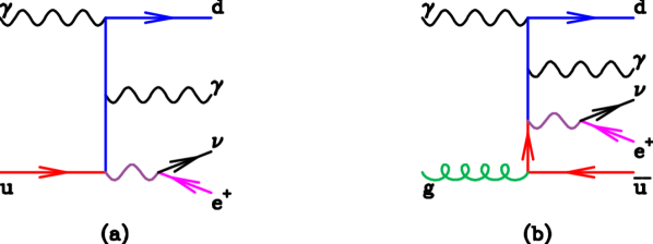
Figure 3: Representative photon-induced diagrams (a) for the process in Eq. (58) and (b) for the process in Eq. (59).

that are shown in Fig. 3. The singularity associated with the initial-state splitting $\gamma\to q\bar{q}$ is absorbed into the quark parton distribution function (pdf) in the $\overline{MS}$ scheme, in accordance with the treatment of the photon pdf in the LUX determination Manohar:2016nzj ; Manohar:2017eqh . For the process shown in Eq. (59) initial-state singularities for the splitting $g\to q\bar{q}$ are also absorbed in the same way. Our numerical results for processes with incoming photons are given in section 6.

5.2 Electroweak virtual corrections

The principal ingredient needed for the next step in evaluating the radiative corrections are the one-loop corrections to the Born-level process due to the exchange of $W,Z$ and $\gamma$. The numerical results for the electroweak corrections to the processes in Eqs. (56,57) have been obtained using the Recola library Actis:2016mpe ; Denner:2017wsf . The Recola library supplies results in three different renormalization schemes,

• the $\alpha(G_{\mu})$ scheme, where $\alpha=\sqrt{2}G_{\mu}/\pi M_{W}^{2}(1-M_{W}^{2}/M_{Z}^{2})$, which includes universal terms associated with the renormalization of the weak mixing angle;

• the $\alpha(0)$ scheme, where $\alpha$ is fixed by the measured value at $p^{2}=0$;

• the $\alpha(M_{Z})$ scheme, where $\alpha$ is fixed by the value at $p^{2}=M_{Z}^{2}$, taking into account the running from $p^{2}=0$ to $p^{2}=M_{Z}^{2}$, which at low $p^{2}$ is inadequately treated in perturbation theory.

Since the $W\gamma$ process involves both a real photon and $W$ bosons we use a hybrid scheme in which the photon is treated in the $\alpha(0)$ scheme but all remaining powers of $\alpha$ (including factors associated with the radiation of additional real or virtual photons) are considered in the $\alpha(G_{\mu})$-scheme. Since we work in dimensional regularization, we note that the translation between $\alpha(0)$ and $\alpha(G_{\mu})$ schemes involves the addition of singular terms – single poles in $\epsilon$ – as well as a finite difference. Clearly, we must also modify our earlier specification of the parameter setup by replacing one power of $\alpha\equiv\alpha(G_{\mu})$ by $\alpha(0)=1/137.036$, resulting in all cross-sections being reduced by a factor $\alpha(0)/\alpha(G_{\mu})=0.965$. All the cross sections quoted in section 6 have this rescaling already applied.

6 Numerical results for 7 and 13 TeV

6.1 Comparison with CMS at 7 TeV

In this section we compare the CMS results Chatrchyan:2013fya based on 5.0 fb^-1 of $\sqrt{s}=7$ TeV data with our predictions. The CMS results are not cross sections in the fiducial region, but rather have been corrected for the geometric and kinematic acceptance of the detector.

Note that, compared to the earlier NLO predictions from MCFM reported in Ref. Chatrchyan:2013fya , the ones here differ in multiple respects. As detailed earlier, here we have used the complex-mass scheme and slightly different electroweak parameters (including a non-diagonal CKM matrix), updated the PDF set (to NNPDF3.0, instead of CTEQ6.6), and used a different central scale choice ($\sqrt{M_{W}^{2}+(p_{T}^{\gamma})^{2}}$, cf. Eq. (49), instead of $M_{W}$), and scale variation (a 9-point variation about the central choice instead of previously a common variation in opposite directions only). Furthermore, anticipating the inclusion of electroweak corrections we replace a single power of $\alpha(G_{\mu})$ in all predictions by $\alpha(0)$, as discussed in the previous section. In addition, our photon isolation is rendered theoretically viable by the hybrid isolation scheme, rather than having recourse to a non-perturbative fragmentation function. The parameters for the hybrid scheme defined in Eqs. (51, 52) are,

$$\epsilon_{s}=0.5,\;\;n=1,\;\;R_{s}=0.1,\;\;\epsilon_{f}=0.0025,\;\;E_{T}^{f}=2.2~{}\mbox{GeV},\;\;R_{f}=0.4\,,$$ (60)

in order to mimic the HCAL photon isolation cut in Ref. Chatrchyan:2013fya . Our theoretical results with the input parameters as described in this paragraph are given in Table 5.

Process	$p_{T}^{\gamma}(min)$	$\sigma_{\text{NLO}}$ [pb]	$\sigma_{\text{NNLO}}$ [pb]	$\sigma_{\text{NNLO}}/\sigma_{\text{NLO}}$
$pp\to e^{+}\nu\gamma$	$15$ [GeV]	$17.98^{+0.77}_{-1.00}$	$19.23^{+0.14}_{-0.41}$	1.070
$pp\to e^{-}\bar{\nu}\gamma$	$15$ [GeV]	$12.43^{+0.54}_{-0.71}$	$13.35^{+0.10}_{-0.28}$	1.074
$pp\to e^{+}\nu\gamma$	$60$ [GeV]	$0.369^{+0.032}_{-0.026}$	$0.451^{+0.021}_{-0.019}$	1.22
$pp\to e^{-}\bar{\nu}\gamma$	$60$ [GeV]	$0.247^{+0.023}_{-0.019}$	$0.314^{+0.017}_{-0.014}$	1.27
$pp\to e^{+}\nu\gamma$	$90$ [GeV]	$0.117^{+0.013}_{-0.010}$	$0.144^{+0.008}_{-0.007}$	1.23
$pp\to e^{-}\bar{\nu}\gamma$	$90$ [GeV]	$0.072^{+0.009}_{-0.007}$	$0.095^{+0.006}_{-0.006}$	1.32

Table 5: Our theoretical predictions for $e^{+}\nu\gamma$ and $e^{-}\bar{\nu}\gamma$ at $\sqrt{s}=7$ TeV. The ratio $\sigma_{\text{NNLO}}/\sigma_{\text{NLO}}$ is given without uncertainty, to illustrate the trend with $p_{T}^{\gamma}(min)\,$.

A comparison between the theoretical predictions and CMS measurements, for these three different values of the minimum photon $p_{T}$, is shown in Table 6. Since the CMS measurement is not in a fiducial region and suffers from rather large systematic errors we do not present the effect of electroweak corrections here, but postpone such a discussion until the following section.

$\sigma(pp\to e^{+}\nu\gamma)+\sigma(pp\to e^{-}\bar{\nu}\gamma)$	NLO [pb]	NNLO [pb]	CMS Experiment [pb]
$\sigma(p_{T}^{\gamma}>15~{}{\rm GeV})$	$30.41^{+1.31}_{-1.72}$	$32.58^{+0.24}_{-0.69}$	$37.0\pm 0.8\pm 4.0\pm 0.8$
$\sigma(p_{T}^{\gamma}>60~{}{\rm GeV})$	$0.616^{+0.055}_{-0.045}$	$0.765^{+0.039}_{-0.035}$	$0.76\pm 0.05\pm 0.08\pm 0.02$
$\sigma(p_{T}^{\gamma}>90~{}{\rm GeV})$	$0.189^{+0.021}_{-0.016}$	$0.238^{+0.014}_{-0.013}$	$0.20\pm 0.03\pm 0.04\pm 0.01$

Table 6: NLO and NNLO predictions for cross sections at $\sqrt{s}=7$ TeV, for comparison with the values measured by the CMS experiment Chatrchyan:2013fya . The experimental result is the average of the cross section to electrons and the cross section to muons. The errors on the experimental results are statistical, systematic and luminosity respectively. All results have a cut $\Delta R^{l\gamma}>0.7$.

In order to probe the radiation zero that occurs at $y_{\gamma}^{\star}=0$ (centre-of-mass frame) it is easiest to construct a boost-invariant difference of rapidities between the lepton and the photon. Weighting this by the charge of the lepton results in the “signed rapidity difference”, the quantity used in the original Tevatron probes of this phenomenon. This quantity has also been measured in Ref. Chatrchyan:2013fya in the fiducial region defined by additional acceptance cuts on the leptons and photon. For the sake of comparison, we show corresponding predictions for this quantity based on the electron-channel cuts shown in Table 7, and after the application of a veto on any jets observed in the region $p_{T}>30$ GeV, $|\eta|<4.4$ using the anti-$k_{T}$ clustering algorithm with $R=0.4$. The transverse cluster mass of the photon, lepton and missing $E_{T}$ (neutrino) system ($M_{T}(\ell\gamma E_{T}^{\rm{miss}})$) is defined by,

$$M_{T}(\ell\gamma E_{T}^{\rm{miss}})=\left[\left(M_{\ell\gamma}^{2}+|\vec{p}_{T}(\gamma)+\vec{p}_{T}(\ell)|^{2}\right)^{\frac{1}{2}}+E_{T}^{\rm{miss}}\right]^{2}-\left|\vec{p}_{T}(\gamma)+\vec{p}_{T}(\ell)+\vec{E}_{T}^{\rm{miss}}\right|^{2}\,.$$ (61)

$|\eta^{\gamma}|<2.5$	$p^{\gamma}_{T}>25$ GeV
$|\eta^{\ell}|<2.5$, excluding $1.44<|\eta^{\ell}|<1.57$	$p^{\ell}>35$ GeV
$\Delta R^{\ell\gamma}>0.7$	$M_{T}(\ell\gamma E_{T}^{\rm{miss}})>110$ GeV

Table 7: Fiducial cuts for theoretical predictions of the signed rapidity difference at 7 TeV.

Our results are shown in Figure 4, where the NLO and NNLO predictions also indicate the uncertainties obtained by scale variation. After the large correction from LO to NLO, for this set of cuts there do not appear to be significant further corrections at NNLO and the scale uncertainties somewhat overlap. However, as is clear from the lower panel of Figure 4, the shape of the NNLO prediction does differ slightly from the NLO one. These predictions appear to be in reasonable agreement with the experimental results of Figure 7 in Ref. Chatrchyan:2013fya .

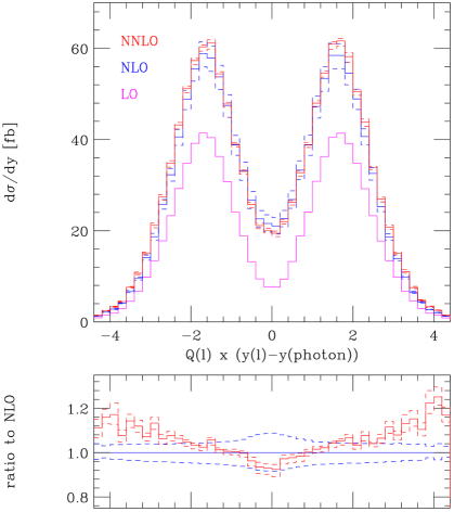
Figure 4: Signed rapidity difference between the lepton and the photon, after the application of the cuts detailed in Table 7 and the jet veto described in the text. The scale variation uncertainties are shown at NLO and NNLO. The lower panel shows the ratio of the NLO and NNLO results, including the uncertainty bands, to the central NLO result.

6.2 MCFM projections for $\sqrt{s}=13$ TeV

In this section we make projections for 13 TeV. We first consider the overall cross section in a fiducial region using the cuts shown in Table 8 taken from Ref. Sirunyan:2021zud . The fiducial region is further reduced by demanding that the leptons and photons are isolated. In Ref. Sirunyan:2021zud a lepton or photon is considered isolated if the sum of the $p_{T}$ of all stable particles within $\Delta R=0.4$, divided by the $p_{T}$ of the lepton or photon, is less than 0.5.

$|\eta^{\gamma}|<2.5$	$p^{\gamma}_{T}>25$ GeV
$|\eta^{\ell}|<2.5$	$p^{\ell}>25$ GeV
$\Delta R^{\ell\gamma}>0.5$

Table 8: Fiducial cuts imposed for calculations of the total rate at 13 TeV.

In our numerical work we follow a procedure that is close to the procedure used in experiments. We compute the inclusive cross section with the anti-$k_{T}$ jet algorithm and identify jets by clustering with $R=0.4$ and demanding $p_{T}({\rm jet})$ > 12.5 GeV. We subsequently check to see whether any jet axes lie within a cone of $\Delta R$=0.4 of the lepton and then reject the event if the scalar sum of any such jet $p_{T}$’s is greater than $0.5\times p_{T}^{l}$. For isolation of the photon we again use a hybrid procedure, with smooth cone parameters (c.f. Eq. (51)),

$$\epsilon_{s}=0.5,\qquad n=1,\qquad R_{s}=0.1\,,$$ (62)

and fixed-cone isolation parameters (c.f. Eq. (52)) taken from Ref. Sirunyan:2021zud ,

$$\epsilon_{f}=0.5,\qquad E_{T}^{f}=0,\qquad R_{f}=0.4\,.$$ (63)

Under these cuts our results are shown in Table 9. We note that the NNLO results lie outside the band of values predicted on the basis of scale variation in the NLO result. Summing both charges in Table 9 we obtain predictions for the cross section in the fiducial region for both electrons and muons (ignoring any feed-down from $\tau$ decays),

Process	$\sigma_{\text{NLO}}$ [pb]	$\sigma_{\text{NNLO}}$ [pb]	$\sigma_{\text{NNLO}}/\sigma_{\text{NLO}}$
$pp\to\nu e^{+}\gamma+pp\to\nu\mu^{+}\gamma$	$5.40^{+0.56}_{-0.56}$	$6.73^{+0.31}_{-0.36}$	1.25
$pp\to e^{-}\bar{\nu}\gamma+pp\to\mu^{-}\bar{\nu}\gamma$	$4.81^{+0.52}_{-0.52}$	$5.96^{+0.28}_{-0.33}$	1.24

Table 9: Theoretical predictions for $\sqrt{s}=13$ TeV using cuts of Table 8 and the isolation cuts described in the text. The ratio $\sigma_{\text{NNLO}}/\sigma_{\text{NLO}}$, given without an uncertainty, indicates that the corrections are still substantial at NNLO.

$$\sigma_{{\rm NLO}}(e^{\pm}\nu\gamma+\mu^{\pm}\nu\gamma) = 10.21^{+1.08}_{-1.08}~{}\text{pb},$$ (64)

$$\sigma_{{\rm NNLO}}(e^{\pm}\nu\gamma+\mu^{\pm}\nu\gamma) = 12.69^{+0.59}_{-0.69}~{}\text{pb}.$$ (65)

The only experimental result at $\sqrt{s}=13$ TeV reported so far is the sum of the cross sections for electrons and muons of both charges,

$$\sigma=15.58\pm 0.05\pm 0.73\pm 0.15~{}\text{pb}$$ (66)

from Ref. Sirunyan:2021zud , where the uncertainties are, respectively, statistical, systematic and related to theoretical inputs.

The NNLO prediction given above is smaller than the experimental measurement by about $20\%$. However a comparison with this data requires a correction for the feed down from the $W\to\tau\nu$ channel, which is present in the result in Eq. (66) but not included in our theoretical rates. We think that this correction is best performed by the experimental collaborations, based on the well-modelled properties of $\tau$ decay.

However in order to get an idea of the order of magnitude of this correction we have studied the number of additional events that may be produced from $\tau$-lepton decays using the Herwig Monte Carlo Bahr:2008pv . The $17\%$ branching ratio of the $\tau$-lepton to electrons and muons sets an upper limit on the size of this correction. However, the leptons of the first two generations coming from $\tau$ decay are much softer than primary leptons, and less frequently isolated. Our studies with Herwig, combining a NLO calculation with the effects of the parton shower, indicate that less than $2\%$ of the produced $\tau$-leptons end up in the CMS event sample. This source of additional events therefore seems unlikely to account for the difference between the theoretical prediction in Eq. (65) and the measured cross-section in Eq. (66).

Finally we turn to the inclusion of electroweak corrections. For the EW corrections to the LO process in Eq. (56) we summarize their effect by using a relative factor $\delta_{EW}$ that is defined by,

$$\delta_{EW}^{q\bar{q}}=\frac{\sigma_{EW}}{\sigma_{LO}}\,,$$ (67)

where both numerator and denominator are computed using the same (LUX) pdf set. This form allows electroweak effects to be incorporated in a QCD-corrected calculation of any order in a straightforward manner. We find the relative correction factors,

$$\delta_{EW}^{q\bar{q}}(\nu\ell^{+}\gamma)=-0.013\,,\;\;\delta_{EW}^{q\bar{q}}(\ell^{-}\bar{\nu}\gamma)=-0.012\,.$$ (68)

Since the photon-initiated process shown in Eq. (58) represents a new partonic channel we do not expect its effects to factorize in the same way. We therefore present the corrections from this channel normalized to the NNLO cross section,

$$\delta_{EW}^{q\gamma}=\frac{\sigma_{EW}}{\sigma_{\text{NNLO}}}\,.$$ (69)

In this way we find,

$$\delta_{EW}^{q\gamma}(\nu\ell^{+}\gamma)=+0.011\,,\;\;\delta_{EW}^{q\gamma}(\ell^{-}\bar{\nu}\gamma)=+0.010\,.$$ (70)

Considered in this way, these two contributions essentially cancel and, taken together, do not represent a substantial further correction to the rate. Indeed, the biggest impact of the inclusion of the electroweak corrections results from the coupling factor change, $\alpha(G_{\mu})\to\alpha(0)$. Electroweak corrections to the $O(\alpha_{s})$ channels represented by Eqs. (57) and  (59) can only be defined in the presence of a jet and their effect on the inclusive rate cannot be directly inferred from the calculations we have performed in this work. Results for these channels will be presented in the following section.

6.3 Differential distributions

We now provide a set of predictions suitable for a possible future measurement of this process at 13 TeV. For this we adopt a slightly different set of cuts, as detailed in Table 10.

$|\eta^{\gamma}|<2.5$	$p^{\gamma}_{T}>30$ GeV
$|\eta^{\ell}|<2.5$	$p^{\ell}_{T}>30$ GeV
$\Delta R^{l\gamma}>0.7$	$E_{T}^{\rm{miss}}>40$ GeV

Table 10: Fiducial cuts imposed for the calculation of differential distributions at 13 TeV.

We use the same lepton and photon isolation requirements as in the previous section, but for this case we identify jets with,

$$p_{T}(\mbox{jet})>30~{}\mbox{GeV}\,,\qquad|\eta(\mbox{jet})|<2.5\,.$$ (71)

All plots in this section sum the contributions of $e^{+}\nu\gamma$ and $e^{-}\bar{\nu}\gamma$. The theoretical result for muons will be identical.

We first show predictions for some basic quantities: the photon rapidity (Figure 5) and the angular separation between the photon and the lepton, $\Delta R^{\ell\gamma}$ (Figure 6). The enormous corrections to the total cross section are reflected as a practically-uniform shift in the photon rapidity distribution, while the shape of the $\Delta R^{\ell\gamma}$ distribution is modified at NNLO. The scale uncertainties, also shown in the figures, do not overlap between NLO and NNLO. This is to be expected because of the effectively leading order nature of a large part of the $O(\alpha_{s})$ contribution.

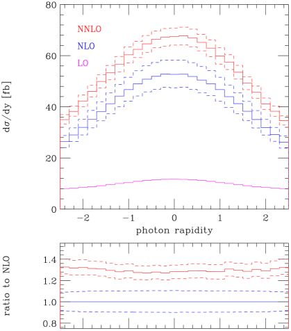
Figure 5: Distribution of the photon rapidity at 13 TeV. The NNLO and NLO histograms display the error estimates, obtained via a 9-point scale variation, and the lower panel displays the ratio of the NLO and NNLO predictions to the central NLO result.

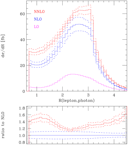
Figure 6: $\Delta R(\ell,\gamma)$ distribution at 13 TeV. The NNLO and NLO histograms display the error estimates, obtained via a 9-point scale variation, and the lower panel displays the ratio of the NLO and NNLO predictions to the central NLO result.

As already discussed in our presentation of results at 7 TeV, the signature of the radiation zero for the $W\gamma$ process is the signed rapidity difference between the lepton and the photon. As shown in Figure 7, the effect of the radiation zero – a depletion in the central region at LO – is almost completely eliminated at NLO. As already indicated, it can be partially restored by applying a jet veto (i.e. so that any event containing a jet as defined in Eq. (71) is removed) and applying a cut on the transverse cluster mass (c.f. Eq. 61). Our prediction at 13 TeV, after applying a jet veto and demanding that $M_{T}(\ell\gamma E_{T}^{\rm{miss}})>150$ GeV, is shown in Figure 8. In this case, in contrast to 7 TeV, the extent of the dip that reflects the radiation zero is changed from NLO to NNLO. This reflects the difficulty in capturing the effects of a jet veto in fixed-order perturbation theory, particularly in the presence of higher-order corrections that are significantly larger at 13 TeV than 7 TeV.

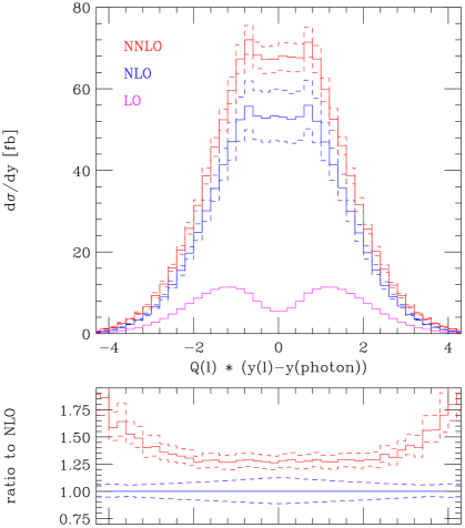
Figure 7: Signed rapidity difference between the lepton and the photon at 13 TeV. The NNLO and NLO histograms display the error estimates, obtained via a 9-point scale variation, and the lower panel displays the ratio of the NLO and NNLO predictions to the central NLO result.

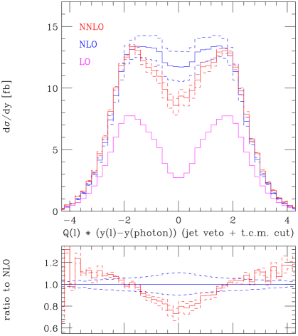
Figure 8: Signed rapidity difference between the lepton and the photon at 13 TeV, after additional cuts to veto jets and require $M_{T}(\ell\gamma E_{T}^{\rm{miss}})>150$ GeV. The NNLO and NLO histograms display the error estimates, obtained via a 9-point scale variation, and the lower panel displays the ratio of the NLO and NNLO predictions to the central NLO result.

Lastly, we turn to two distributions that directly probe a wide range of energy scales: the photon $p_{T}$ (Figure 9) and the transverse cluster mass distribution (Figure 10). Although we have seen that the net effect of electroweak corrections to the rate in the fiducial volume is small, these distributions are particularly sensitive to their effects.

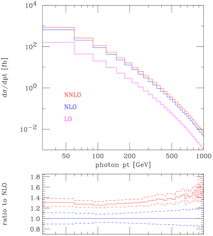
Figure 9: $p_{T}^{\gamma}$ distribution at 13 TeV. The lower panel displays the ratio of the NLO and NNLO predictions, including error estimates obtained via a 9-point scale variation, to the central NLO result.

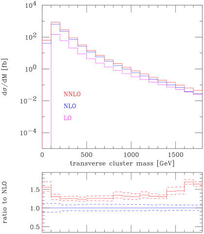
Figure 10: Cluster transverse mass of the ($\ell$–$\gamma$–$\nu$) system, defined in Eq. (61), at 13 TeV. The lower panel displays the ratio of the NLO and NNLO predictions, including error estimates obtained via a 9-point scale variation, to the central NLO result.

6.4 Numerical results for electroweak corrections

We illustrate the size of electroweak corrections that can be expected under this set of cuts by considering their effect on the $p_{T}^{\gamma}$ distribution. We plot this distribution out to values of $1$ TeV since this corresponds, under these cuts, to about $200$ $\ell^{\pm}\nu\gamma$ events in the full 3 ab^-1 HL-LHC data set.

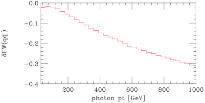
Figure 11: Relative electroweak corrections to the $q\bar{q}$-initiated process in Eq. (56).

Corrections from the process in Eq. (56) are shown in Fig. 11, as a factor relative to the LO process (c.f. Eq. (67)). Overall the effect on the total rate is,

$$\delta_{EW}^{q\bar{q}}=-0.013\,,\;\;$$ (72)

but the corrections to the $p_{T}^{\gamma}$ distribution are much more significant in the tail. The size of the corrections is very similar to that already observed, albeit under slightly different cuts, in Ref. Denner:2014bna . Relative corrections from the process in Eq. (57) are shown in Fig. 12, for three different choices of the jet $p_{T}$ threshold – $15$, $40$ and $100$ GeV – normalized to the $O(\alpha_{s})$ (leading order) result for the $W\gamma$-jet process. Although the size of the corrections differs in the first few bins of this distribution, for $p_{T}^{\gamma}>200$ GeV all three curves are similar. This indicates that, although the effect on the inclusive $W\gamma$ rate is hard to estimate, corrections from this channel are important at large $p_{T}^{\gamma}$ and should be taken into account. The similarity of the electroweak corrections between the $O(1)$ (Fig. 11) and $O(\alpha_{s})$ (Fig. 12) channels suggests that a multiplicative approach to incorporating the effects of electroweak corrections into QCD-corrected predictions correctly captures these effects, particularly at high energies. An estimate of the mixed QCD-EW corrections, that are not correctly captured in such a scheme, can be inferred from the difference between Figs. 11 and 12. A definitive statement cannot be made, of course, until a proper calculation of the mixed QCD-EW corrections is performed.

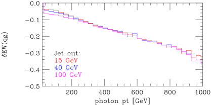
Figure 12: Relative electroweak corrections to the $O(\alpha_{s})$ process in Eq. (57), for three values of the minimum jet $p_{T}$.

Results for $\delta^{q\gamma}_{EW}$, resulting from the $q\gamma\to W\gamma q$-channel in Eq. (58), are shown in Fig. 13. Under these cuts the effect on the full rate is,

$$\delta_{EW}^{q\gamma}=+0.013\,,\;\;$$ (73)

although in the distribution this manifests as a $4\%$ enhancement for $p_{T}^{\gamma}=1$ TeV. As expected the application of a jet veto, with jets defined according to Eq. (71), somewhat reduces the size of the corrections, especially at large $p_{T}^{\gamma}$, and the size of the electroweak corrections to the overall rate becomes,

$$\delta_{EW}^{q\gamma}({\rm jet~{}veto})=+0.009\,.\;\;$$ (74)

Although this channel results in an enhancement of the cross-section we note that, compared to previous calculations of these effects Denner:2014bna , the size of the corrections is much reduced. This is partially due to the fact that here we have normalized to NNLO predictions; replacing the denominator in Eq. (69) with the LO result would increase $\delta_{EW}^{q\gamma}$ by about a factor of $4$. The remaining large difference with respect to the results of Ref. Denner:2014bna simply reflects the improved determination of the photon distribution in the LUX pdf set Manohar:2016nzj ; Manohar:2017eqh compared to NNPDF2.3QED Ball:2013hta , the pdf set used in Ref. Denner:2014bna . The photon pdf in the LUX determination is significantly smaller at large $x$ than the central result in NNPDF2.3QED, although the two are compatible within the (large) uncertainties of the latter.

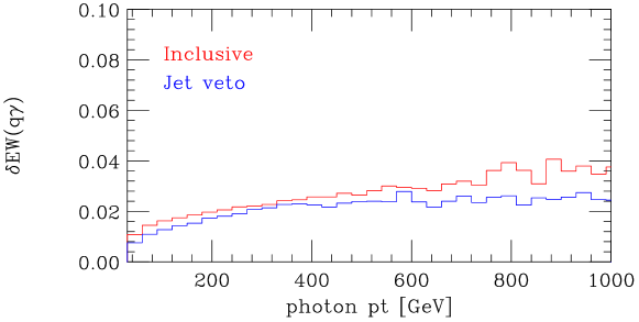
Figure 13: Relative electroweak corrections resulting from the $q\gamma$-initiated process in Eq. (58).

We find that, after factorization of singularities into the pdfs, corrections from the process in Eq. (59) are negligible, below the per-mille level, across all of the kinematic range. This is due to the fact that this channel does not open a new and significant kinematic configuration, unlike the processes in Eqs. (57) and (58). This lends further credence to the suggestion that corrections from photon-induced channels should be applied additively, i.e. according to Eq. (69).

Finally, we note that application of a jet veto will reduce the effect of all these corrections, as demonstrated explicitly in Fig. 13 for the $q\gamma$-initiated contributions. This merely indicates that, especially for the case of electroweak corrections, the effect of higher orders depends delicately on the experimental measurement for which the theoretical prediction is being made.

7 Conclusions

We have presented NNLO results for the processes $pp\to e^{+}\nu_{e}\gamma$ and $pp\to e^{-}\bar{\nu}_{e}\gamma$ calculated using a jettiness slicing scheme. This allows us to construct the cross section for an electron of either charge, accompanied by a photon,

$$\sigma=\sigma(pp\to e^{+}\nu_{e}\gamma)+\sigma(pp\to e^{-}\bar{\nu}_{e}\gamma)$$ (75)

which is the quantity usually quoted by experiment. Our analytic formulae are valid for the process $pp\to e^{+}\nu_{e}\gamma$. The extension to the opposite charge process $pp\to e^{-}\bar{\nu}_{e}\gamma$ can be performed by exchange, and, since the leptons are considered to be massless, the extension to $\mu^{+}$ and $\mu^{-}$ is immediate.

Our numerical results show full agreement with the results of the MATRIX collaboration, performed using a different slicing method. We have included the effects of CKM rotation, which are found to be numerically small. Generically we can see that the NNLO effects are large and (in the main) positive, (e.g. at $\sqrt{s}=13$ TeV they are about $20\%$), and that the scale dependence at NLO gives little hint that such a correction is to be expected. However the destructive interference in the lowest order contribution does lead one to suspect that the NNLO calculation for $W\gamma$ might behave more like an NLO correction than an NNLO correction, a suspicion that is borne out by our detailed calculations.

Our results indicate that the NNLO effects can play a substantial role in the description of the radiation zero at $\sqrt{s}=13$ TeV. The clearest signature of the radiation zero requires a veto on jet activity. It is well-known that such vetoes can generate large logarithms, suggesting that a more accurate description of the distributions might benefit from a resummation of large logarithms, as was performed for the $Z\gamma$ process in Ref. Becher:2020ugp .

We have also considered electroweak effects of various sources. As far as the total cross section is concerned we find that the decrease in the cross section due to the replacement of one power of $\alpha$ changes the cross section by a factor $\alpha(0)/\alpha(M_{Z}^{2})\approx 0.965$. The incoming photon $\gamma q$ process corrects the lowest order process by 0.9–1.3%, depending on the photon $p_{T}$ cut and the presence (or not) of a jet veto, c.f. Eqs. (70), (73) and (74). In contrast the $\gamma g$ process gives a negligible effect. Virtual and real photon emission corrections to the total cross section can only be evaluated for the $q\bar{q}$ process and are negative and give about $-1.3\%$, c.f. Eqs. (68) and (72). As is well known the virtual and real photon emission corrections become large at high $p_{T}$, as much as $-30\%$ and $+4\%$ respectively, at photon $p_{T}=1$ TeV.

We are of the opinion that, compared to the $Z\gamma$ process, the $W\gamma$ process has not as yet received the attention from experimenters it deserves. When decays to final state leptons are taken into account the $Z\gamma$ and $W\gamma$ processes have about the same cross section. Of course the $Z\gamma$ process has a final state without missing energy, and it is also of interest because of its role in the search for the rare Higgs boson decay, $H\to Z\gamma$. However the importance of the triple weak boson coupling in the $W\gamma$ process should not be underestimated.

Appendix A Spinor algebra

All results are presented using the standard notation for the kinematic invariants of the process,

$$s_{ij}=(p_{i}+p_{j})^{2}\,,s_{ijk}=(p_{i}+p_{j}+p_{k})^{2}\,,s_{ijkl}=(p_{i}+p_{j}+p_{k}+p_{l})^{2}\,.$$ (76)

and the Gram determinant,

$$\Delta_{ij,kl}=(s_{ijkl}-s_{ij}-s_{kl})^{2}-4s_{ij}s_{kl}\,.$$ (77)

We express the amplitudes in terms of spinor products defined as,

$$\left\langle ij\right\rangle=\bar{u}_{-}(p_{i})u_{+}(p_{j}),\;\;\;\left[ij\right]=\bar{u}_{+}(p_{i})u_{-}(p_{j}),\;\;\;\left\langle ij\right\rangle\left[ji\right]=2p_{i}\cdot p_{j},\;\;\;$$ (78)

and we further define the spinor sandwiches for light-like momenta $j$ and $k$,

$$\langle i|(j+k)|l] = \left\langle ij\right\rangle\left[jl\right]+\left\langle ik\right\rangle\left[kl\right],$$

$$[i|(j+k)|l\rangle = \left[ij\right]\left\langle jl\right\rangle+\left[ik\right]\left\langle kl\right\rangle.$$ (79)

In the Weyl representation the spinor solutions of the massless Dirac equation are,

$$u_{+}(p)=|p\rangle=\left[\begin{matrix}\sqrt{p^{+}}\cr\sqrt{p^{-}}e^{i\varphi_{p}}\cr 0\cr 0\cr\end{matrix}\right],\hskip 8.53581ptu_{-}(p)=|p]=\left[\begin{matrix}0\cr 0\cr\sqrt{p^{-}}e^{-i\varphi_{p}}\cr-\sqrt{p^{+}}\cr\end{matrix}\right],$$ (80)

where

$$e^{\pm i\varphi_{p}}\ \equiv\ \frac{p^{1}\pm ip^{2}}{\sqrt{(p^{1})^{2}+(p^{2})^{2}}}\ =\ \frac{p^{1}\pm ip^{2}}{\sqrt{p^{+}p^{-}}}\ ,\qquad p^{\pm}\ =\ p^{0}\pm p^{3}.$$ (81)

In this representation the Dirac conjugate spinors are,

$$\bar{u}_{+}(p)=[p|\equiv u_{+}^{\dagger}(p)\gamma^{0}=\left[0,0,\begin{matrix}\sqrt{p^{+}},\sqrt{p^{-}}e^{-i\varphi_{p}}\cr\end{matrix}\right],$$ (82)

$$\bar{u}_{-}(p)=\langle p|\equiv u_{-}^{\dagger}(p)\gamma^{0}=\left[\sqrt{p^{-}}e^{i\varphi_{p}},-\sqrt{p^{+}},0,0\right].$$ (83)

Appendix B Integral functions in the amplitudes

Due to the linear vanishing of $\ln(r)$ as $r\rightarrow 1$ it is convenient to introduce the $\mathrm{L}_{0}$ and $\mathrm{L}_{1}$ functions Bern:1993mq in order to make explicit the absence of certain singularities

$$\mathrm{L}_{0}(r)=\frac{\ln(r)}{1-r}\;,\quad\quad\mathrm{L}_{1}(r)=\frac{\mathrm{L}_{0}(r)+1}{1-r}=\frac{\ln(r)}{(1-r)^{2}}+\frac{1}{1-r}\,.$$ (84)

In particular, $r\rightarrow\{0,1,\infty\}$ are the three physically relevant limits, which can be respectively written as the following Maclaurin series for $\mathrm{L}_{0}$

$$\lim_{r\rightarrow 0}\;\mathrm{L}_{0}(r) \approx \vphantom{\frac{1}{1}}\ln(r)+r\,\ln(r)+\dots\;,$$ (85)

$$\lim_{x\rightarrow 0}\;\mathrm{L}_{0}(1+x) \approx -1+\frac{x}{2}-\frac{x^{2}}{3}+\dots\;,$$ (86)

$$\lim_{y\rightarrow 0}\;\mathrm{L}_{0}(1/y) \approx \vphantom{\frac{1}{1}}-y\,\ln(1/y)-y^{2}\,\ln(1/y)+\dots\;,$$ (87)

and for $\mathrm{L}_{1}$

$$\lim_{r\rightarrow 0}\;\mathrm{L}_{1}(r) \approx \vphantom{\frac{1}{1}}(1+\ln(r))+r\,(1+2\ln(r))+\dots\;,$$ (88)

$$\lim_{x\rightarrow 0}\;\mathrm{L}_{1}(1+x) \approx -\frac{1}{2}+\frac{x}{3}-\frac{x^{2}}{4}+\dots\;,$$ (89)

$$\lim_{y\rightarrow 0}\;\mathrm{L}_{1}(1/y) \approx \vphantom{\frac{1}{1}}-y+y^{2}(-1+\ln(1/y))+\dots\;.$$ (90)

Both $\mathrm{L}_{0}$ and $\mathrm{L}_{1}$ display a logarithmic divergence for $r\rightarrow 0$, are regular for $r\rightarrow 1$ and vanish linearly for $r\rightarrow\infty$. Let us consider the commonly seen case where $r=s_{ijk}/s_{ij}$. Then, the three limits $r\rightarrow\{0,1,\infty\}$ correspond respectively to $\{s_{ijk},\langle k|i+j|k],s_{ij}\}\rightarrow 0$, due to the following relation

$$s_{ijk}=s_{ij}+s_{ik}+s_{jk}=s_{ij}+\langle k|i+j|k]\;.$$ (91)

Sums of Mandelstam variables of the form $\langle k|i+j|k]$ appear as poles in scalar bubble integral coefficients. However, these poles are spurious when considering complete one-loop amplitudes. We can use the $\mathrm{L}_{0}$ and $\mathrm{L}_{1}$ functions to explicitly remove them. If $\langle k|i+j|k]$ appears as a simple pole we can write

$$\frac{\mathrm{L}_{0}(\frac{-s_{ijk}}{-s_{ij}})}{s_{ij}}=-\ln(\frac{-s_{ijk}}{-s_{ij}})\frac{1}{\langle k|i+j|k]}\,,$$ (92)

which is regular in $\langle k|i+j|k]\rightarrow 0$ and logarithmically divergent for $\{s_{ijk},s_{ij}\}\rightarrow 0$. If $\langle k|i+j|k]$ appears as a double pole, then there will be a corresponding rational piece where it appears as a simple pole. This allows to write the following expression

$$\frac{\mathrm{L}_{1}(\frac{-s_{ijk}}{-s_{ij}})}{s_{ij}}=\ln(\frac{-s_{ijk}}{-s_{ij}})\frac{s_{ij}}{\langle k|i+j|k]^{2}}-\frac{1}{\langle k|i+j|k]}\,,$$ (93)

which is regular in $\{\langle k|i+j|k],s_{ij}\}\rightarrow 0$ and logarithmically divergent for $s_{ijk}\rightarrow 0$. Alternatively the following combination may also appear

$$\frac{\mathrm{L}_{1}(\frac{-s_{ij}}{-s_{ijk}})}{s_{ijk}}=\ln(\frac{-s_{ij}}{-s_{ijk}})\frac{s_{ijk}}{\langle k|i+j|k]^{2}}+\frac{1}{\langle k|i+j|k]}\,,$$ (94)

which is regular for $\{\langle k|i+j|k],s_{ijk}\}\rightarrow 0$ and logarithmically divergent for $s_{ij}\rightarrow 0$.

The following transcendental functions are also needed

$$\mathrm{Ls}_{-1}(r_{1},r_{2}) = \mathrm{Li}_{2}(1-r_{1})+\mathrm{Li}_{2}(1-r_{2})+\ln r_{1}\,\ln r_{2}-{\pi^{2}\over 6}\,,$$ (95)

$$\mathrm{Ls}_{0}(r_{1},r_{2}) = {1\over(1-r_{1}-r_{2})}\,\mathrm{Ls}_{-1}(r_{1},r_{2})\,,$$ (96)

$$\mathrm{Ls}_{1}(r_{1},r_{2}) = {1\over(1-r_{1}-r_{2})}\,\left[\mathrm{Ls}_{0}(r_{1},r_{2})+\mathrm{L}_{0}(r_{1})+\mathrm{L}_{0}(r_{2})\right]\,,$$ (97)

$$\mathrm{Ls}^{2{\rm m}h}_{-1}(s,t;m_{1}^{2},m_{2}^{2})=-\mathrm{Li}_{2}\left(1-{m_{1}^{2}\over t}\right)-\mathrm{Li}_{2}\left(1-{m_{2}^{2}\over t}\right)-{1\over 2}\ln^{2}\left({-s\over-t}\right)$$ (98)

$$+ {1\over 2}\ln\left({-s\over-m_{1}^{2}}\right)\ln\left({-s\over-m_{2}^{2}}\right)+\biggl{[}{1\over 2}(s-m_{1}^{2}-m_{2}^{2})+{m_{1}^{2}m_{2}^{2}\over t}\biggr{]}I_{3}^{3{\rm m}}(s,m_{1}^{2},m_{2}^{2})\,,$$

$$\mathop{\rm\widetilde{Ls}}\nolimits^{2{\rm m}h}_{-1}(s,t;m_{1}^{2},m_{2}^{2}) = -\mathrm{Li}_{2}\left(1-{m_{1}^{2}\over t}\right)-\mathrm{Li}_{2}\left(1-{m_{2}^{2}\over t}\right)-{1\over 2}\ln^{2}\left({-s\over-t}\right)$$ (99)

$$+ {1\over 2}\ln\left({-s\over-m_{1}^{2}}\right)\ln\left({-s\over-m_{2}^{2}}\right)\,,$$

$$\mathrm{Ls}^{2{\rm m}e}_{-1}(s,t;m_{1}^{2},m_{3}^{2}) = -\mathrm{Li}_{2}\left(1-{m_{1}^{2}\over s}\right)-\mathrm{Li}_{2}\left(1-{m_{1}^{2}\over t}\right)-\mathrm{Li}_{2}\left(1-{m_{3}^{2}\over s}\right)-\mathrm{Li}_{2}\left(1-{m_{3}^{2}\over t}\right)$$ (101)

$$\quad+\mathrm{Li}_{2}\left(1-{m_{1}^{2}m_{3}^{2}\over st}\right)-{1\over 2}\ln^{2}\left({-s\over-t}\right)\;.$$

where the dilogarithm is

$$\mathrm{Li}_{2}(x)=-\int_{0}^{x}dy\,{\ln(1-y)\over y}\,.$$ (102)

and $I_{3}^{3{\rm m}}$ is a three-mass scalar triangle integral, defined according to Appendix II of Ref. Bern:1997sc ,

$$I_{3}^{3{\rm m}}(s_{12},s_{34},s_{56})=\int_{0}^{1}da_{1}\,\int_{0}^{1}da_{2}\,\int_{0}^{1}da_{3}\,\frac{\delta(1-a_{1}-a_{2}-a_{3})}{[-s_{12}a_{1}a_{2}-s_{34}a_{2}a_{3}-s_{56}a_{3}a_{1}+i\epsilon]}.$$ (103)

Note that this has the opposite sign to commonly-used definitions of scalar integrals, such as in QCDLoop Ellis:2007qk .

Appendix C Six-parton process at one-loop order

C.1 Radiation for $u$ and $d$ quarks

The one-loop corrections to the process

$$0\rightarrow\bar{u}(p_{1})+d(p_{2})+\nu_{e}(p_{3})+e^{+}(p_{4})+g(p_{5})+g(p_{6})$$ (104)

have been presented in Ref. Bern:1997sc . Although certain terms that we need can be derived from these results, that is not true for all terms, so we present the full analytic terms here. A computer readable representation of the results in this appendix accompanies the arXiv version of this article.

C.1.1 Leading colour, $5_{\gamma}^{+},6_{g}^{+}$

$$A^{u}_{\mathrm{lc}}(5_{\gamma}^{+},6_{g}^{+})=\frac{\left\langle 23\right\rangle^{2}\left[43\right]}{\left\langle 15\right\rangle\left\langle 26\right\rangle\left\langle 56\right\rangle}\,\mathrm{Ls}_{-1}\left(\frac{-s_{15}}{-s_{16}},\frac{-s_{156}}{-s_{16}}\right)$$

$$+\frac{\left\langle 12\right\rangle\left\langle 23\right\rangle^{2}\left[34\right]}{\left\langle 15\right\rangle\left\langle 16\right\rangle\left\langle 25\right\rangle\left\langle 26\right\rangle}\,\left(\mathrm{Ls}_{-1}^{2\mathrm{me}}\left(s_{126},s_{156};s_{16},s_{34}\right)+\mathrm{Ls}_{-1}\left(\frac{-s_{16}}{-s_{26}},\frac{-s_{126}}{-s_{26}}\right)\right)$$

$$+\frac{\left\langle 12\right\rangle\left[45\right]}{2\left\langle 15\right\rangle\left\langle 16\right\rangle\left\langle 26\right\rangle}\left[3\,\left\langle 23\right\rangle\,\mathrm{L}_{0}\left(\frac{-s_{126}}{-s_{34}}\right)+\left\langle 35\right\rangle\langle 2|1+6|5]\,\frac{\mathrm{L}_{1}\left(\frac{-s_{126}}{-s_{34}}\right)}{s_{34}}\right]$$

$$+\frac{1}{2}\frac{\left\langle 12\right\rangle\left[16\right]}{\left\langle 15\right\rangle\left\langle 16\right\rangle\left\langle 25\right\rangle}\Bigg{(}\left\langle 23\right\rangle(3\left\langle 13\right\rangle\left[34\right]-2\left\langle 15\right\rangle\left[45\right])-\left\langle 13\right\rangle\langle 2|1+5|4]\Bigg{)}\,\frac{\mathrm{L}_{0}\left(\frac{-s_{126}}{-s_{26}}\right)}{s_{26}}$$

$$-\frac{\left\langle 12\right\rangle^{2}\left\langle 13\right\rangle\left[16\right]\left[14\right]}{2\left\langle 15\right\rangle\left\langle 16\right\rangle\left\langle 25\right\rangle}\,\frac{\mathrm{L}_{1}\left(\frac{-s_{126}}{-s_{26}}\right)}{s_{26}}+\frac{\left\langle 12\right\rangle^{2}\left\langle 23\right\rangle\left[14\right]}{2\left\langle 15\right\rangle\left\langle 16\right\rangle\left\langle 25\right\rangle\left\langle 26\right\rangle}$$

$$+\frac{\left\langle 12\right\rangle\left\langle 23\right\rangle\left[45\right]}{\left\langle 15\right\rangle\left\langle 16\right\rangle\left\langle 26\right\rangle}+\frac{\left\langle 23\right\rangle\left[56\right]\langle 1|2+3|4]}{2\left\langle 15\right\rangle\left\langle 16\right\rangle s_{234}}$$

$$+V_{\mathrm{lc}}(s_{126})\,A^{u}_{\mathrm{tree}}(1_{\bar{u}}^{+},2_{d}^{-},3_{\nu}^{-},4_{\ell}^{+},5_{\gamma}^{+},6_{g}^{+})$$ (105)

In this formula the term containing the poles in $\epsilon$ is given by,

$$V_{\mathrm{lc}}(s_{x})=-\frac{1}{\epsilon^{2}}\left[\left(\frac{\mu^{2}}{-s{{}_{16}}}\right)^{\epsilon}+\left(\frac{\mu^{2}}{-s{{}_{26}}}\right)^{\epsilon}\right]-\frac{3}{2\epsilon}\left(\frac{\mu^{2}}{-s_{x}}\right)^{\epsilon}-3\,,$$ (106)

and the corresponding leading-order subamplitude has been given in Eq.(21).

$$A^{d}_{\mathrm{lc}}(5_{\gamma}^{+},6_{g}^{+})=$$

$$-\frac{\left\langle 12\right\rangle^{3}\left\langle 35\right\rangle^{2}\left[43\right]}{\left\langle 15\right\rangle^{3}\left\langle 16\right\rangle\left\langle 25\right\rangle\left\langle 26\right\rangle}\,\mathrm{Ls}_{-1}^{2\mathrm{me}}\left(s_{126},s_{256};s_{26},s_{34}\right)$$

$$+\frac{\left(\left\langle 23\right\rangle\left\langle 56\right\rangle(\left\langle 25\right\rangle\left\langle 36\right\rangle+\left\langle 26\right\rangle\left\langle 35\right\rangle)-(\left\langle 25\right\rangle\left\langle 36\right\rangle)^{2}\right)\left[43\right]}{\left\langle 16\right\rangle\left\langle 25\right\rangle\left\langle 56\right\rangle^{3}}\,\mathrm{Ls}_{-1}\left(\frac{-s_{26}}{-s_{25}},\frac{-s_{256}}{-s_{25}}\right)$$

$$-\frac{\left\langle 12\right\rangle^{3}\left[14\right]\langle 3|2+6|1]}{2\left\langle 16\right\rangle\left\langle 15\right\rangle\left\langle 26\right\rangle\left\langle 25\right\rangle}\,\frac{\mathrm{L}_{1}\left(\frac{-s_{126}}{-s_{26}}\right)}{s_{26}}+\frac{\left\langle 12\right\rangle\left\langle 25\right\rangle\left[45\right]^{2}\left\langle 43\right\rangle}{2\left\langle 16\right\rangle\left\langle 15\right\rangle\left\langle 26\right\rangle}\,\frac{\mathrm{L}_{1}\left(\frac{-s_{126}}{-s_{34}}\right)}{s_{34}}$$

$$+\frac{\left\langle 12\right\rangle^{3}\left[14\right]^{2}\left\langle 43\right\rangle}{2\left\langle 16\right\rangle\left\langle 15\right\rangle\left\langle 26\right\rangle\left\langle 25\right\rangle}\,\frac{\mathrm{L}_{1}\left(\frac{-s_{134}}{-s_{34}}\right)}{s_{34}}-\frac{\left\langle 26\right\rangle\left\langle 35\right\rangle^{2}\left[56\right]^{2}\left[43\right]}{2\left\langle 15\right\rangle\left\langle 56\right\rangle}\,\frac{\mathrm{L}_{1}\left(\frac{-s_{26}}{-s_{256}}\right)}{s_{256}^{2}}$$

$$-\frac{\left\langle 25\right\rangle\left\langle 36\right\rangle^{2}\left[56\right]^{2}\left[43\right]}{2\left\langle 16\right\rangle\left\langle 56\right\rangle}\,\frac{\mathrm{L}_{1}\left(\frac{-s_{25}}{-s_{256}}\right)}{s_{256}^{2}}-\frac{\left\langle 12\right\rangle^{2}\left[16\right]\left[43\right]}{\left\langle 15\right\rangle\left\langle 16\right\rangle\left\langle 25\right\rangle}\left(\frac{\left\langle 13\right\rangle\left\langle 35\right\rangle}{\left\langle 15\right\rangle}+\frac{\langle 3|1+5|4]}{2\left[34\right]}\right)\,\frac{\mathrm{L}_{0}\left(\frac{-s_{126}}{-s_{26}}\right)}{s_{26}}$$

$$+\frac{\left\langle 12\right\rangle\left[45\right](\left\langle 12\right\rangle\left\langle 35\right\rangle-\left\langle 23\right\rangle\left\langle 15\right\rangle)}{\left\langle 15\right\rangle^{2}\left\langle 16\right\rangle\left\langle 26\right\rangle}\,\mathrm{L}_{0}\left(\frac{-s_{126}}{-s_{34}}\right)-\frac{\left\langle 12\right\rangle^{3}\left\langle 35\right\rangle\left[14\right]}{\left\langle 16\right\rangle\left\langle 15\right\rangle^{2}\left\langle 26\right\rangle\left\langle 25\right\rangle}\,\mathrm{L}_{0}\left(\frac{-s_{134}}{-s_{34}}\right)$$

$$+\frac{\left\langle 35\right\rangle^{2}\left[56\right]\left[43\right]\left(\left\langle 12\right\rangle\left\langle 56\right\rangle+\left\langle 15\right\rangle\left\langle 26\right\rangle\right)}{\left\langle 15\right\rangle^{2}\left\langle 56\right\rangle^{2}}\,\frac{\mathrm{L}_{0}\left(\frac{-s_{256}}{-s_{26}}\right)}{s_{26}}+\frac{\left\langle 36\right\rangle\left[56\right]\left[43\right]\left(\left\langle 26\right\rangle\left\langle 35\right\rangle-\left\langle 23\right\rangle\left\langle 56\right\rangle\right)}{\left\langle 16\right\rangle\left\langle 56\right\rangle^{2}}\,\frac{\mathrm{L}_{0}\left(\frac{-s_{256}}{-s_{25}}\right)}{s_{25}}$$

$$-\frac{\left\langle 12\right\rangle\left\langle 23\right\rangle\left[46\right]}{2\left\langle 16\right\rangle\left\langle 15\right\rangle\left\langle 25\right\rangle}\,\ln\left(\frac{-s_{126}}{-s_{26}}\right)+\frac{\left\langle 12\right\rangle\left\langle 23\right\rangle\left[43\right]}{\left\langle 15\right\rangle\left\langle 16\right\rangle\left\langle 26\right\rangle}\left(\frac{3\left\langle 23\right\rangle}{2\left\langle 25\right\rangle}-\frac{\left\langle 13\right\rangle}{\left\langle 15\right\rangle}\right)\,\ln\left(\frac{-s_{256}}{-s_{126}}\right)$$

$$+\frac{\left\langle 13\right\rangle\left[56\right]\langle 2|1+3|4]}{2\left\langle 16\right\rangle\left\langle 15\right\rangle s_{256}}-\frac{\left\langle 12\right\rangle\left\langle 23\right\rangle\left[45\right]}{2\left\langle 16\right\rangle\left\langle 15\right\rangle\left\langle 26\right\rangle}$$ (107)

C.1.2 Subeading colour, $5_{\gamma}^{+},6_{g}^{+}$

$$A^{u}_{\mathrm{sl}}(5_{\gamma}^{+},6_{g}^{+})=\frac{\left\langle 25\right\rangle^{2}\left\langle 36\right\rangle^{2}\left[34\right]}{\left\langle 15\right\rangle\left\langle 26\right\rangle\left\langle 56\right\rangle^{3}}\,\mathrm{Ls}_{-1}^{2\mathrm{me}}\left(s_{125},s_{126};s_{12},s_{34}\right)$$

$$-\frac{\left\langle 23\right\rangle^{2}\left[34\right]}{\left\langle 16\right\rangle\left\langle 25\right\rangle\left\langle 56\right\rangle}\,\left(\mathrm{Ls}_{-1}^{2\mathrm{me}}\left(s_{126},s_{156};s_{16},s_{34}\right)+\mathrm{Ls}_{-1}\left(\frac{-s_{16}}{-s_{12}},\frac{-s_{126}}{-s_{12}}\right)\right)$$

$$+\frac{\left\langle 23\right\rangle^{2}\left[34\right]}{\left\langle 15\right\rangle\left\langle 26\right\rangle\left\langle 56\right\rangle}\,\left(\mathrm{Ls}_{-1}^{2\mathrm{me}}\left(s_{125},s_{156};s_{15},s_{34}\right)+\mathrm{Ls}_{-1}\left(\frac{-s_{15}}{-s_{12}},\frac{-s_{125}}{-s_{12}}\right)\right)$$

$$+\frac{\left\langle 12\right\rangle^{2}\left\langle 36\right\rangle(\left\langle 12\right\rangle\left[43\right]\left\langle 36\right\rangle-\left\langle 26\right\rangle\left\langle 15\right\rangle\left[54\right])}{\left\langle 15\right\rangle\left\langle 16\right\rangle^{3}\left\langle 25\right\rangle\left\langle 26\right\rangle}\,\mathrm{Ls}_{-1}\left(\frac{-s_{12}}{-s_{26}},\frac{-s_{126}}{-s_{26}}\right)$$

$$+\frac{\left\langle 26\right\rangle\left[46\right]^{2}\left\langle 43\right\rangle}{\left\langle 15\right\rangle\left\langle 56\right\rangle}\,\frac{\mathrm{L}_{1}\left(\frac{-s_{125}}{-s_{34}}\right)}{s_{34}}-\frac{\left\langle 12\right\rangle\left\langle 26\right\rangle\left\langle 36\right\rangle\left[16\right]\left[46\right]}{\left\langle 16\right\rangle\left\langle 25\right\rangle\left\langle 56\right\rangle}\,\frac{\mathrm{L}_{1}\left(\frac{-s_{126}}{-s_{12}}\right)}{s_{12}}$$

$$+\frac{\left\langle 12\right\rangle^{2}\left\langle 13\right\rangle\left[16\right]\left[14\right]}{2\left\langle 15\right\rangle\left\langle 16\right\rangle\left\langle 25\right\rangle}\,\frac{\mathrm{L}_{1}\left(\frac{-s_{126}}{-s_{26}}\right)}{s_{26}}-\frac{\left\langle 12\right\rangle\left\langle 25\right\rangle\left[45\right]^{2}\left\langle 43\right\rangle}{2\left\langle 15\right\rangle\left\langle 16\right\rangle\left\langle 26\right\rangle}\,\frac{\mathrm{L}_{1}\left(\frac{-s_{126}}{-s_{34}}\right)}{s_{34}}$$

$$-\frac{\left\langle 12\right\rangle\left\langle 35\right\rangle^{2}\left[15\right]\left[43\right]}{\left\langle 15\right\rangle\left\langle 56\right\rangle^{2}}\,\frac{\mathrm{L}_{0}\left(\frac{-s_{125}}{-s_{12}}\right)}{s_{12}}-\frac{\left\langle 25\right\rangle\left\langle 36\right\rangle\left[46\right]}{\left\langle 15\right\rangle\left\langle 56\right\rangle^{2}}\,\mathrm{L}_{0}\left(\frac{-s_{125}}{-s_{34}}\right)$$

$$-\frac{\left\langle 12\right\rangle\left[16\right]}{\left\langle 16\right\rangle\left\langle 56\right\rangle}\left(\frac{\left\langle 13\right\rangle\left\langle 26\right\rangle^{2}\left[24\right]}{\left\langle 16\right\rangle\left\langle 25\right\rangle}+\frac{\left\langle 13\right\rangle\left\langle 26\right\rangle\left[14\right]}{\left\langle 25\right\rangle}-\frac{\left\langle 36\right\rangle\langle 2|1+3|4]}{\left\langle 25\right\rangle}+\frac{\left\langle 36\right\rangle^{2}\left[34\right]}{\left\langle 56\right\rangle}\right)\,\frac{\mathrm{L}_{0}\left(\frac{-s_{126}}{-s_{12}}\right)}{s_{12}}$$

$$-\frac{\left\langle 12\right\rangle\left[16\right]}{\left\langle 16\right\rangle\left\langle 25\right\rangle}\left(\frac{\left\langle 12\right\rangle\left\langle 13\right\rangle\left\langle 26\right\rangle\left[24\right]}{\left\langle 15\right\rangle\left\langle 16\right\rangle}+\frac{\left\langle 13\right\rangle\left\langle 23\right\rangle\left[34\right]}{2\left\langle 15\right\rangle}-\frac{3\left\langle 13\right\rangle\langle 2|1+5|4]}{2\left\langle 15\right\rangle}-\left\langle 23\right\rangle\left[45\right]\right)\,\frac{\mathrm{L}_{0}\left(\frac{-s_{126}}{-s_{26}}\right)}{s_{26}}$$

$$+\frac{\left[45\right]}{\left\langle 15\right\rangle\left\langle 16\right\rangle}\left(\frac{\left\langle 16\right\rangle\left\langle 25\right\rangle\left\langle 35\right\rangle}{\left\langle 56\right\rangle^{2}}-\frac{\left\langle 12\right\rangle\left\langle 23\right\rangle}{\left\langle 26\right\rangle}\right)\,\mathrm{L}_{0}\left(\frac{-s_{126}}{-s_{34}}\right)+\frac{\left\langle 23\right\rangle\left\langle 35\right\rangle\left[43\right]}{\left\langle 15\right\rangle\left\langle 56\right\rangle^{2}}\,\ln\left(\frac{-s_{126}}{-s_{125}}\right)$$

$$-\frac{\left\langle 23\right\rangle\langle 1|2+3|4]}{2\left\langle 56\right\rangle s_{234}}\left(\frac{\left[15\right]}{\left\langle 16\right\rangle}-\frac{\left[16\right]}{\left\langle 15\right\rangle}\right)-\frac{\left\langle 23\right\rangle\langle 2|1+3|4]}{2\left\langle 16\right\rangle\left\langle 25\right\rangle\left\langle 56\right\rangle}$$

$$+\left(V_{\mathrm{sl}}+\frac{1}{2}\right)\,A^{u}_{\mathrm{tree}}(1_{\bar{u}}^{+},2_{d}^{-},3_{\nu}^{-},4_{\ell}^{+},5_{\gamma}^{+},6_{g}^{+})$$ (108)

The contribution that includes the poles in $\epsilon$ is,

$$V_{\mathrm{sl}}=\frac{1}{\epsilon^{2}}\left(\frac{\mu^{2}}{-s{{}_{12}}}\right)^{\epsilon}+\frac{3}{2\epsilon}\left(\frac{\mu^{2}}{-s{{}_{126}}}\right)^{\epsilon}+3\,.$$ (109)

$$A^{d}_{\mathrm{sl}}(5_{\gamma}^{+},6_{g}^{+})=\frac{\left\langle 26\right\rangle^{2}\left\langle 35\right\rangle^{2}\left[43\right]}{\left\langle 16\right\rangle\left\langle 25\right\rangle\left\langle 56\right\rangle^{3}}\,\mathrm{Ls}_{-1}^{2\mathrm{me}}\left(s_{126},s_{125};s_{12},s_{34}\right)$$

$$-\frac{\left\langle 12\right\rangle^{2}\left\langle 35\right\rangle^{2}\left[43\right]}{\left\langle 15\right\rangle^{2}\left\langle 56\right\rangle}\left[\frac{1}{\left\langle 15\right\rangle\left\langle 26\right\rangle}\,\mathrm{Ls}_{-1}^{2\mathrm{me}}\left(s_{126},s_{256};s_{26},s_{34}\right)-\frac{1}{\left\langle 16\right\rangle\left\langle 25\right\rangle}\,\mathrm{Ls}_{-1}\left(\frac{-s_{12}}{-s_{25}},\frac{-s_{125}}{-s_{25}}\right)\right]$$

$$+\frac{\left\langle 12\right\rangle^{2}\left\langle 36\right\rangle}{\left\langle 16\right\rangle^{3}\left\langle 25\right\rangle\left\langle 56\right\rangle}\left[\left\langle 36\right\rangle\left[43\right]\,\mathrm{Ls}_{-1}^{2\mathrm{me}}\left(s_{125},s_{256};s_{25},s_{34}\right)+\langle 6|1+2|4]\,\mathrm{Ls}_{-1}\left(\frac{-s_{12}}{-s_{26}},\frac{-s_{126}}{-s_{26}}\right)\right]$$

$$-\frac{\left\langle 25\right\rangle\left\langle 36\right\rangle^{2}\left[56\right]^{2}\left[43\right]}{2\left\langle 56\right\rangle\left\langle 16\right\rangle}\,\frac{\mathrm{L}_{1}\left(\frac{-s_{25}}{-s_{134}}\right)}{s_{134}^{2}}+\frac{\left\langle 26\right\rangle\left\langle 35\right\rangle^{2}\left[56\right]^{2}\left[43\right]}{2\left\langle 56\right\rangle\left\langle 15\right\rangle}\,\frac{\mathrm{L}_{1}\left(\frac{-s_{26}}{-s_{134}}\right)}{s_{134}^{2}}-\frac{\left\langle 26\right\rangle^{2}\left[46\right]^{2}\left\langle 43\right\rangle}{\left\langle 25\right\rangle\left\langle 56\right\rangle\left\langle 16\right\rangle}\,\frac{\mathrm{L}_{1}\left(\frac{-s_{125}}{-s_{34}}\right)}{s_{34}}$$

$$-\frac{\left\langle 12\right\rangle^{2}\left\langle 13\right\rangle\left[16\right]\left[14\right]}{2\left\langle 25\right\rangle\left\langle 15\right\rangle\left\langle 16\right\rangle}\,\frac{\mathrm{L}_{1}\left(\frac{-s_{126}}{-s_{26}}\right)}{s_{26}}-\frac{\left\langle 25\right\rangle\left\langle 12\right\rangle\left[45\right]^{2}\left\langle 43\right\rangle}{2\left\langle 26\right\rangle\left\langle 15\right\rangle\left\langle 16\right\rangle}\,\frac{\mathrm{L}_{1}\left(\frac{-s_{126}}{-s_{34}}\right)}{s_{34}}$$

$$-\frac{\left\langle 26\right\rangle^{2}\left[46\right]\langle 3|1+2|6]}{\left\langle 25\right\rangle\left\langle 56\right\rangle\left\langle 16\right\rangle}\,\frac{\mathrm{L}_{1}\left(\frac{-s_{126}}{-s_{12}}\right)}{s_{12}}-\frac{\left\langle 12\right\rangle^{3}\left[14\right]^{2}\left\langle 43\right\rangle}{2\left\langle 25\right\rangle\left\langle 26\right\rangle\left\langle 15\right\rangle\left\langle 16\right\rangle}\,\frac{\mathrm{L}_{1}\left(\frac{-s_{134}}{-s_{34}}\right)}{s_{34}}$$

$$+\frac{\left\langle 12\right\rangle\left\langle 13\right\rangle^{2}\left[15\right]\left[43\right]}{\left\langle 15\right\rangle\left\langle 16\right\rangle^{2}}\,\frac{\mathrm{L}_{0}\left(\frac{-s_{125}}{-s_{25}}\right)}{s_{25}}+\frac{\left\langle 26\right\rangle\left\langle 36\right\rangle\left[46\right](\left\langle 25\right\rangle\left\langle 16\right\rangle-\left\langle 12\right\rangle\left\langle 56\right\rangle)}{\left\langle 16\right\rangle^{2}\left\langle 25\right\rangle\left\langle 56\right\rangle^{2}}\,\mathrm{L}_{0}\left(\frac{-s_{125}}{-s_{34}}\right)$$

$$+\frac{\left\langle 35\right\rangle^{2}\left\langle 12\right\rangle\left[15\right]\left[43\right]}{\left\langle 56\right\rangle^{2}\left\langle 15\right\rangle}\,\frac{\mathrm{L}_{0}\left(\frac{-s_{125}}{-s_{12}}\right)}{s_{12}}+\left[45\right]\left(\frac{\left\langle 25\right\rangle\left\langle 35\right\rangle\left\langle 12\right\rangle}{\left\langle 26\right\rangle\left\langle 56\right\rangle\left\langle 15\right\rangle^{2}}-\frac{\left\langle 26\right\rangle\left\langle 35\right\rangle}{\left\langle 56\right\rangle^{2}\left\langle 16\right\rangle}+\frac{\left\langle 23\right\rangle\left\langle 12\right\rangle}{\left\langle 26\right\rangle\left\langle 15\right\rangle\left\langle 16\right\rangle}\right)\,\mathrm{L}_{0}\left(\frac{-s_{126}}{-s_{34}}\right)$$

$$+\frac{\left\langle 12\right\rangle\left[16\right]\left[43\right]}{\left\langle 15\right\rangle\left\langle 16\right\rangle\left\langle 25\right\rangle}\left(\frac{\left\langle 26\right\rangle\left\langle 13\right\rangle\left[46\right]}{2\left[34\right]}+\frac{\left\langle 35\right\rangle\left\langle 12\right\rangle\left\langle 13\right\rangle}{\left\langle 15\right\rangle}-\frac{\left\langle 36\right\rangle\left\langle 12\right\rangle\langle 1|2+6|4]}{\left\langle 16\right\rangle\left[34\right]}\right)\,\frac{\mathrm{L}_{0}\left(\frac{-s_{126}}{-s_{26}}\right)}{s_{26}}$$

$$+\frac{\left\langle 26\right\rangle\left\langle 36\right\rangle\left\langle 12\right\rangle\left[46\right]}{\left\langle 16\right\rangle\left\langle 56\right\rangle}\left(\frac{\left[12\right]}{\left\langle 56\right\rangle}+\frac{\langle 1|2+6|1]}{\left\langle 25\right\rangle\left\langle 16\right\rangle}\right)\,\frac{\mathrm{L}_{0}\left(\frac{-s_{126}}{-s_{12}}\right)}{s_{12}}-\frac{\left\langle 36\right\rangle^{2}\left\langle 12\right\rangle\left[56\right]\left[43\right]}{\left\langle 56\right\rangle\left\langle 16\right\rangle^{2}}\,\frac{\mathrm{L}_{0}\left(\frac{-s_{134}}{-s_{25}}\right)}{s_{25}}$$

$$-\frac{\left\langle 35\right\rangle^{2}\left\langle 12\right\rangle\left[56\right]\left[43\right]}{\left\langle 56\right\rangle\left\langle 15\right\rangle^{2}}\,\frac{\mathrm{L}_{0}\left(\frac{-s_{134}}{-s_{26}}\right)}{s_{26}}+\frac{\left\langle 12\right\rangle^{2}\left[14\right]}{\left\langle 15\right\rangle\left\langle 16\right\rangle\left\langle 26\right\rangle}\left(\frac{\left\langle 36\right\rangle\left\langle 12\right\rangle}{\left\langle 25\right\rangle\left\langle 16\right\rangle}+\frac{\left\langle 13\right\rangle}{\left\langle 15\right\rangle}\right)\,\mathrm{L}_{0}\left(\frac{-s_{134}}{-s_{34}}\right)$$

$$+\frac{(\left\langle 36\right\rangle\left\langle 12\right\rangle\left\langle 56\right\rangle-\left\langle 26\right\rangle\left\langle 16\right\rangle\left\langle 35\right\rangle)}{\left\langle 25\right\rangle\left\langle 16\right\rangle^{2}\left\langle 56\right\rangle^{2}}\,\left(\left\langle 12\right\rangle\left[14\right]\,\ln\left(\frac{-s_{126}}{-s_{12}}\right)+\left\langle 23\right\rangle\left[43\right]\,\ln\left(\frac{-s_{126}}{-s_{125}}\right)\right)$$

$$+\frac{\left\langle 12\right\rangle\left\langle 23\right\rangle\left[43\right]}{\left\langle 15\right\rangle\left\langle 16\right\rangle}\left(\frac{3\left\langle 23\right\rangle}{2\left\langle 25\right\rangle\left\langle 26\right\rangle}-\frac{\left\langle 13\right\rangle}{\left\langle 25\right\rangle\left\langle 16\right\rangle}-\frac{\left\langle 13\right\rangle}{\left\langle 26\right\rangle\left\langle 15\right\rangle}\right)\,\ln\left(\frac{-s_{126}}{-s_{134}}\right)$$

$$+\frac{\left[56\right]\left[43\right]}{\left\langle 16\right\rangle s_{134}}\left(\frac{\left\langle 26\right\rangle\left\langle 13\right\rangle\left[14\right]}{\left\langle 56\right\rangle\left[34\right]}-\frac{\left\langle 23\right\rangle\left\langle 36\right\rangle}{\left\langle 56\right\rangle}+\frac{\left\langle 13\right\rangle\langle 2|1+3|4]}{2\left\langle 15\right\rangle\left[34\right]}\right)-\frac{\left\langle 23\right\rangle\left\langle 12\right\rangle\langle 2|1+5|4]}{2\left\langle 25\right\rangle\left\langle 26\right\rangle\left\langle 15\right\rangle\left\langle 16\right\rangle}$$ (110)

C.1.3 Leading colour, $5_{\gamma}^{-},6_{g}^{+}$

$$A^{d}_{\mathrm{lc}}(5_{\gamma}^{-},6_{g}^{+})=s_{34}\Bigg{[}$$

$$\Big{(}\frac{\left[14\right]^{2}\left\langle 25\right\rangle^{2}}{s_{256}\left\langle 26\right\rangle\left[34\right]\langle 6|2+5|1]}+\frac{\langle 3|2+5|6]^{2}}{\left[25\right]s_{256}\left\langle 34\right\rangle\langle 1|2+6|5]}\Big{)}\,\mathrm{Ls}_{-1}^{2\mathrm{mh}}\left(s_{16},s_{256};s_{25},s_{34}\right)$$

$$-\frac{\left\langle 12\right\rangle\langle 2|1+6|4]^{2}}{\left\langle 16\right\rangle\left[34\right]\left\langle 26\right\rangle\langle 1|2+6|5]\langle 2|1+6|5]}\,\mathrm{Ls}_{-1}^{2\mathrm{mh}}\left(s_{25},s_{126};s_{16},s_{34}\right)$$

$$+\frac{\langle 3|2+5|6]^{2}}{\left[25\right]s_{256}\left\langle 34\right\rangle\langle 1|2+6|5]}\,\mathrm{Ls}_{-1}\left(\frac{-s_{25}}{-s_{26}},\frac{-s_{256}}{-s_{26}}\right)$$

$$-\frac{\langle 2|1+6|4](\left\langle 26\right\rangle\left[61\right]\left\langle 13\right\rangle-\left\langle 12\right\rangle\left[14\right]\left\langle 34\right\rangle)}{\langle 1|2+6|5]\left[15\right]\left\langle 16\right\rangle\left\langle 26\right\rangle s_{34}}\,\mathrm{Ls}_{-1}\left(\frac{-s_{16}}{-s_{26}},\frac{-s_{126}}{-s_{26}}\right)$$

$$+\Big{(}\frac{2\left\langle 25\right\rangle^{2}\langle 3|2+5|6]\left[14\right]}{\left\langle 62\right\rangle s_{256}^{2}}+\frac{\left\langle 12\right\rangle}{\left\langle 62\right\rangle s_{126}s_{256}}\Big{(}\frac{\langle 5|2+6|1]\langle 3|2+5|6]\langle 2|1+6|4]}{\langle 1|2+6|5]}-\left[16\right]\left\langle 25\right\rangle\left\langle 53\right\rangle\left[14\right]\Big{)}\Big{)}$$

$$\times I_{3}^{3m}\left(s_{16},s_{25},s_{34}\right)+\frac{3}{2}\frac{\langle 3|1+4|6]^{2}}{\left[25\right]\left\langle 34\right\rangle\langle 1|2+6|5]s_{134}}\,\Big{(}\ln\left(\frac{-s_{256}}{-s_{26}}\right)-\ln\left(\frac{-s_{34}}{-s_{126}}\right)\Big{)}$$

$$+\frac{3\left\langle 13\right\rangle\left[16\right]\langle 2|1+6|4]+\left\langle 12\right\rangle\left[14\right](\left\langle 35\right\rangle\left[56\right]-\left\langle 34\right\rangle\left[46\right])}{2\left\langle 16\right\rangle\left[15\right]\left\langle 34\right\rangle\left[34\right]\langle 1|2+6|5]}\,\ln\left(\frac{-s_{26}}{-s_{126}}\right)$$

$$-\frac{2\left\langle 13\right\rangle\left[16\right]\langle 3|1+4|6]}{\left\langle 34\right\rangle\left[25\right]\langle 1|2+6|5]s_{134}}\,\mathrm{L}_{0}\left(\frac{-s_{34}}{-s_{134}}\right)-\frac{3\left\langle 35\right\rangle\left\langle 12\right\rangle\langle 2|3+5|4]}{2\left\langle 34\right\rangle\left[34\right]\left\langle 16\right\rangle\left\langle 26\right\rangle\langle 1|2+6|5]}\,\mathrm{L}_{0}\left(\frac{-s_{126}}{-s_{34}}\right)$$

$$+\frac{\left\langle 12\right\rangle^{2}\left[14\right]}{2\left\langle 16\right\rangle\left\langle 26\right\rangle\left[34\right]\langle 1|2+6|5]}\Big{(}\frac{\left[14\right]}{\left[15\right]}-\frac{\left\langle 35\right\rangle}{\left\langle 34\right\rangle}\Big{)}\,\mathrm{L}_{0}\left(\frac{-s_{126}}{-s_{26}}\right)$$

$$-\frac{\left\langle 35\right\rangle\left[56\right]\langle 3|2+5|6]}{\left\langle 26\right\rangle\left\langle 34\right\rangle\left[25\right]\left[26\right]\langle 1|2+6|5]}\,\mathrm{L}_{0}\left(\frac{-s_{256}}{-s_{26}}\right)-\frac{1}{2}\frac{\left\langle 13\right\rangle^{2}\left[16\right]^{2}}{\left[25\right]\left\langle 34\right\rangle\langle 1|2+6|5]s_{134}}\,\mathrm{L}_{1}\left(\frac{-s_{34}}{-s_{134}}\right)$$

$$+\frac{1}{2}\frac{\left\langle 35\right\rangle\left\langle 12\right\rangle\left\langle 25\right\rangle\left[45\right]}{\left\langle 16\right\rangle\left\langle 26\right\rangle\langle 1|2+6|5]s_{126}}\,\mathrm{L}_{1}\left(\frac{-s_{34}}{-s_{126}}\right)+\frac{1}{2}\frac{\left\langle 35\right\rangle^{2}\left[56\right]^{2}}{\left[25\right]\left\langle 34\right\rangle\langle 1|2+6|5]s_{256}}\,\mathrm{L}_{1}\left(\frac{-s_{26}}{-s_{256}}\right)$$

$$+\frac{1}{2\langle 1|2+6|5]}\Big{(}\frac{\langle 3|1+4|6]^{2}}{\left[25\right]\left\langle 34\right\rangle s_{134}}+\frac{\left\langle 12\right\rangle^{2}\left[14\right]^{2}}{\left[34\right]\left[15\right]\left\langle 16\right\rangle\left\langle 26\right\rangle}+\frac{\left[46\right]^{2}}{\left[34\right]\left[25\right]}-\frac{\left\langle 35\right\rangle\left\langle 12\right\rangle\left\langle 23\right\rangle}{\left\langle 34\right\rangle\left\langle 16\right\rangle\left\langle 26\right\rangle}\Big{)}\Bigg{]}$$

$$+V_{\mathrm{lc}}(s_{126})\,A^{d}_{\mathrm{tree}}(1_{\bar{u}}^{+},2_{d}^{-},3_{\nu}^{-},4_{\ell}^{+},5_{\gamma}^{-},6_{g}^{+})$$ (111)

where the corresponding tree-level amplitude has been given in Eq.(26). An alternative form may also be useful for simplification:

$$A^{d}_{\mathrm{tree}}(5_{\gamma}^{-},6_{g}^{+})=$$

$$\frac{1}{\langle 1|2+6|5]}\Bigg{(}\frac{\left\langle 12\right\rangle\left[14\right]\langle 2|1+6|4]\left\langle 43\right\rangle}{\left[15\right]\left\langle 16\right\rangle\left\langle 26\right\rangle}-\frac{\left\langle 13\right\rangle\left[16\right]\langle 2|1+6|4]}{\left[15\right]\left\langle 16\right\rangle}-\frac{\langle 3|1+4|6]^{2}\left[43\right]}{\left[25\right]s_{134}}\Bigg{)}$$ (112)

$$A^{u}_{\mathrm{lc}}(5_{\gamma}^{-},6_{g}^{+})=$$

$$\frac{1}{s_{156}}\Big{(}\frac{\left\langle 34\right\rangle\langle 6|1+5|4]^{2}\langle 5|1+6|2]^{2}}{\left\langle 16\right\rangle\langle 6|1+5|2]^{3}}+\frac{\left\langle 23\right\rangle^{2}\left[16\right]^{2}\left[34\right]}{\langle 2|1+6|5]\left[15\right]}\Big{)}\,\mathrm{Ls}_{-1}^{2\mathrm{mh}}\left(s_{26},s_{156};s_{15},s_{34}\right)$$

$$-\frac{\left\langle 12\right\rangle^{3}\left\langle 34\right\rangle\left[45\right]^{2}s_{126}^{2}}{\left\langle 16\right\rangle\left\langle 62\right\rangle\langle 1|2+6|5]^{3}\langle 2|1+6|5]}\,\mathrm{Ls}_{-1}^{2\mathrm{mh}}\left(s_{15},s_{126};s_{26},s_{34}\right)$$

$$+\frac{\left[16\right]^{2}\left\langle 23\right\rangle^{2}\left[34\right]}{\left[15\right]s_{156}\langle 2|1+6|5]}\,\mathrm{Ls}_{-1}\left(\frac{-s_{15}}{-s_{16}},\frac{-s_{156}}{-s_{16}}\right)$$

$$-\frac{\left[16\right]\langle 2|1+6|4]\left\langle 23\right\rangle}{\left[15\right]\left\langle 16\right\rangle\langle 2|1+6|5]}\,\mathrm{Ls}_{-1}\left(\frac{-s_{16}}{-s_{26}},\frac{-s_{126}}{-s_{26}}\right)$$

$$-\left(T_{\text{sum}}-T_{\text{SL}}\right)\,I_{3}^{3m}\left(s_{15},s_{26},s_{34}\right)+L(5_{\gamma}^{-},6_{g}^{+})$$

$$+V_{\mathrm{lc}}(s_{126})\,A^{u}_{\mathrm{tree}}(1_{\bar{u}}^{+},2_{d}^{-},3_{\nu}^{-},4_{\ell}^{+},5_{\gamma}^{-},6_{g}^{+})$$ (113)

where the triangle coefficient is expressed in terms of,

$$T_{\text{sum}}=s_{34}\Big{[}$$

$$2\frac{\left\langle 15\right\rangle\left[16\right]\left\langle 23\right\rangle\langle 5|1+6|4]}{\left\langle 16\right\rangle s_{234}^{2}}-\frac{\left\langle 12\right\rangle\left[15\right]\left\langle 23\right\rangle\langle 2|1+6|4]\langle 5|1+6|2]}{\left\langle 16\right\rangle\langle 2|1+6|5]\langle 6|1+2|5]s_{234}}$$

$$-2\frac{\left\langle 15\right\rangle\left[16\right]\left\langle 23\right\rangle\left[24\right]\left\langle 56\right\rangle}{\left\langle 16\right\rangle\langle 6|1+5|2]s_{234}}+\frac{\left\langle 12\right\rangle\langle 3|2+5|1]\langle 5|1+6|4]}{\left\langle 16\right\rangle\langle 6|1+2|5]s_{234}}$$

$$-\frac{\left\langle 12\right\rangle\left[26\right]\left\langle 36\right\rangle\left[45\right]\langle 5|2+6|1]}{\langle 1|2+6|5]\langle 6|1+5|2]\langle 6|1+2|5]}+\frac{2\left\langle 26\right\rangle\left[26\right]\langle 1|5|6]\langle 3|1+5|4]\langle 5|2+6|1]}{\langle 1|2+6|5]\langle 6|1+5|2]\,\Delta_{15,26}}$$

$$+\frac{\left\langle 12\right\rangle\left[26\right]\langle 3|1+5|4]\langle 5|2+6|1](s_{12}+s_{25}+s_{16}+s_{56})}{\langle 1|2+6|5]\langle 6|1+5|2]\,\Delta_{15,26}}$$

$$-\frac{\left\langle 12\right\rangle\left[16\right]\left[24\right]\left\langle 36\right\rangle\left\langle 56\right\rangle}{\left\langle 16\right\rangle\langle 6|1+5|2]\langle 6|1+2|5]}+\frac{\left\langle 12\right\rangle\left[14\right]\left\langle 35\right\rangle}{\left\langle 16\right\rangle\langle 6|1+2|5]}\Big{]}$$ (114)

and,

$$T_{\text{SL}}=s_{34}\Big{[}$$

$$+\frac{\left\langle 13\right\rangle\left[56\right]\langle 5|2+6|1]\langle 1|3+5|4](s_{134}-s_{345})(s_{12}-s_{56})}{\langle 1|2+6|5]^{2}\langle 6|1+5|2]\,\Delta_{15,26}}$$

$$+\frac{\left\langle 36\right\rangle\left[45\right]\langle 5|1+2|6](s_{34}-s_{56})}{2\langle 1|2+6|5]\langle 6|1+5|2]\langle 6|1+2|5]}+\frac{\left\langle 13\right\rangle\left[15\right]\left[34\right]\left\langle 36\right\rangle\langle 5|1+2|6]}{\langle 1|2+6|5]\langle 6|1+5|2]\langle 6|1+2|5]}$$

$$-\frac{3\left\langle 15\right\rangle\left[15\right]\left\langle 16\right\rangle\left[26\right]\langle 2|1+5|6]\langle 3|1+5|4]\langle 5|2+6|1](s_{12}+s_{16}+s_{25}+s_{56})}{\langle 1|2+6|5]\langle 6|1+5|2]\,\Delta_{15,26}^{2}}$$

$$-\frac{6\left\langle 15\right\rangle^{2}\left[15\right]\left[25\right]\left\langle 26\right\rangle\left[26\right]\langle 2|1+5|6]\langle 3|1+5|4]\langle 5|2+6|1]}{\langle 1|2+6|5]\langle 6|1+5|2]\,\Delta_{15,26}^{2}}$$

$$+\frac{\left\langle 13\right\rangle\left[46\right]\left\langle 56\right\rangle\left[56\right]\langle 5|2+6|1](s_{134}-s_{345}-s_{24})}{\langle 1|2+6|5]\langle 6|1+5|2]\,\Delta_{15,26}}$$

$$+\frac{2\left[12\right]\left\langle 13\right\rangle\left[56\right]\langle 5|2+6|1]}{\langle 1|2+6|5]\langle 6|1+5|2]\,\Delta_{15,26}}$$

$$\,(-\left\langle 12\right\rangle\left[14\right]\left\langle 15\right\rangle-2\left\langle 12\right\rangle\left[24\right]\left\langle 25\right\rangle-\left\langle 12\right\rangle\left[34\right]\left\langle 35\right\rangle-2\left\langle 13\right\rangle\left\langle 25\right\rangle\left[34\right]+2\left\langle 15\right\rangle\left\langle 25\right\rangle\left[45\right])$$

$$+\frac{\left\langle 13\right\rangle\left\langle 56\right\rangle\left[56\right]\langle 5|2+6|1]}{2\langle 1|2+6|5]\langle 6|1+5|2]\,\Delta_{15,26}}\,(-4\left\langle 12\right\rangle\left[14\right]\left[26\right]-\left\langle 23\right\rangle\left[24\right]\left[36\right]-3\left\langle 24\right\rangle\left[24\right]\left[46\right])$$

$$+\frac{4\left\langle 12\right\rangle\left[12\right]\left\langle 13\right\rangle\left\langle 16\right\rangle\left[16\right]\left[46\right]\langle 5|2+6|1]}{\langle 1|2+6|5]\langle 6|1+5|2]\,\Delta_{15,26}}$$

$$-\frac{\left\langle 12\right\rangle\left\langle 35\right\rangle(\left[12\right]\left[46\right]+\left[14\right]\left[26\right])(s_{134}-s_{345})(s_{125}-s_{156})}{2\langle 1|2+6|5]\langle 6|1+5|2]\,\Delta_{15,26}}$$

$$+\frac{\left\langle 12\right\rangle\left\langle 35\right\rangle(-3\left[12\right]\left[46\right]+\left[14\right]\left[26\right])}{2\langle 1|2+6|5]\langle 6|1+5|2]}+\frac{\left\langle 23\right\rangle\left[45\right]\langle 5|1+2|6]}{\langle 1|2+6|5]\langle 6|1+2|5]}$$

$$+\frac{\left[46\right]\langle 5|2+6|1](4\left\langle 12\right\rangle(\left\langle 35\right\rangle\left[56\right]+\left\langle 13\right\rangle\left[16\right])-\left\langle 13\right\rangle\left\langle 25\right\rangle\left[56\right])}{\langle 1|2+6|5]\,\Delta_{15,26}}$$

$$-\frac{3\left\langle 12\right\rangle\left[16\right]\left\langle 35\right\rangle\left[46\right](s_{134}-s_{345})}{\langle 1|2+6|5]\,\Delta_{15,26}}-\frac{\left[16\right]\left\langle 25\right\rangle\left\langle 35\right\rangle\left[46\right]}{2\,\Delta_{15,26}}\Big{]}$$

$$+\Big{\{}1\leftrightarrow 2,3\leftrightarrow 4,5\leftrightarrow 6,\langle\,\rangle\leftrightarrow[\,]\Big{\}}$$ (115)

The term containing logarithmic functions is,

$$L(5_{\gamma}^{-},6_{g}^{+})=s_{34}\Bigg{[}$$

$$+\frac{1}{\Delta_{15,26}}\frac{\langle 2|1+5|6]\langle 5|2+6|1]\langle 3|1+5|4]}{2\left\langle 34\right\rangle\left[34\right]\langle 1|2+6|5]\langle 6|1+5|2]}\Big{(}\frac{\left\langle 16\right\rangle\,\delta_{15}}{\left\langle 26\right\rangle}-\frac{\left[25\right]\,\delta_{26}}{\left[15\right]}\Big{)}$$

$$-\frac{\left[14\right]\left[26\right]\left\langle 12\right\rangle^{2}\left\langle 13\right\rangle}{2\left[34\right]\left\langle 16\right\rangle\left\langle 34\right\rangle\langle 1|2+6|5]^{2}}\,\mathrm{L}_{0}\left(\frac{-s_{126}}{-s_{26}}\right)-\frac{1}{2}\frac{\left[24\right]^{2}\left\langle 25\right\rangle^{2}s_{234}}{\left\langle 16\right\rangle s_{34}^{2}\left[34\right]\langle 6|1+5|2]}\,\mathrm{L}_{1}\left(\frac{-s_{234}}{-s_{34}}\right)$$

$$+\frac{\left\langle 56\right\rangle\left[46\right]}{\left\langle 16\right\rangle\left[15\right]\left[34\right]\langle 6|1+5|2]}\Big{(}\frac{\left\langle 56\right\rangle\left[15\right]\left[42\right]}{\langle 6|1+5|2]}-2\frac{\langle 5|1+6|4]}{\left\langle 15\right\rangle}\Big{)}\,\mathrm{L}_{0}\left(\frac{-s_{156}}{-s_{15}}\right)$$

$$+\frac{\left[24\right]}{\left\langle 16\right\rangle\left[34\right]\langle 6|1+5|2]s_{34}}\Big{(}(\langle 5|2+3|4]+\left[14\right]\left\langle 15\right\rangle)\left\langle 25\right\rangle+\frac{\left\langle 56\right\rangle\langle 2|1+5|4]\langle 5|1+6|2]}{\langle 6|1+5|2]}\Big{)}\,\mathrm{L}_{0}\left(\frac{-s_{234}}{-s_{34}}\right)$$

$$+\frac{\left\langle 12\right\rangle\left\langle 35\right\rangle}{\left\langle 16\right\rangle\left\langle 26\right\rangle\left\langle 34\right\rangle\langle 1|2+6|5]}\Big{(}\frac{\left[45\right]\left\langle 12\right\rangle\left\langle 34\right\rangle}{\langle 1|2+6|5]}-\frac{\langle 2|1+6|4]}{\left[34\right]}\Big{)}\,\mathrm{L}_{0}\left(\frac{-s_{345}}{-s_{34}}\right)$$

$$-\frac{1}{2}\frac{\left[46\right]^{2}\left\langle 56\right\rangle^{2}s_{156}}{\left[34\right]\left\langle 16\right\rangle s_{15}^{2}\langle 6|1+5|2]}\,\mathrm{L}_{1}\left(\frac{-s_{156}}{-s_{15}}\right)+\frac{1}{2}\frac{\left[34\right]\left\langle 12\right\rangle\left\langle 35\right\rangle^{2}\langle 2|3+4|5]}{\left\langle 16\right\rangle\left\langle 26\right\rangle s_{34}^{2}\langle 1|2+6|5]}\,\mathrm{L}_{1}\left(\frac{-s_{345}}{-s_{34}}\right)$$

$$+\ln\left(\frac{-s_{15}}{-s_{26}}\right)\,\frac{1}{2\,\Delta_{15,26}}\frac{1}{\langle 1|2+6|5]\langle 6|1+5|2]}\Big{(}-12\left[12\right]\left\langle 12\right\rangle\left[16\right]\left\langle 15\right\rangle\langle 3|1+5|4]$$

$$-10\left[12\right]\left\langle 12\right\rangle\left[26\right]\left\langle 25\right\rangle\langle 3|1+5|4]-3\frac{\left\langle 13\right\rangle\left[12\right]\left\langle 35\right\rangle\langle 2|1+5|6](s_{15}-s_{26}-s_{34})}{\left\langle 34\right\rangle}$$

$$+3\frac{\left\langle 13\right\rangle\left[26\right]\left\langle 23\right\rangle\langle 5|2+6|1](s_{15}-s_{26})}{\left\langle 34\right\rangle}-\frac{\left[24\right]\left\langle 15\right\rangle\langle 2|1+5|6]\left[14\right](s_{15}-s_{26})}{\left[34\right]}$$

$$+\frac{\left[24\right]\left\langle 15\right\rangle\langle 2|1+5|6]\left[45\right]\langle 5|2+6|1]}{\left[34\right]}-3\frac{\left[24\right]\left[46\right]\left\langle 12\right\rangle\langle 5|2+6|1](s_{15}-s_{26})}{\left[34\right]}$$

$$-2\frac{\left[45\right]\left[46\right]\left\langle 15\right\rangle\langle 5|2+6|1](s_{15}-s_{26})}{\left[34\right]}+8\langle 3|1|4]\langle 5|1|2]\langle 2|1+5|6]+6\langle 3|1|4]\langle 5|6|2]\langle 2|1+5|6]$$

$$+6\langle 3|5|4]\langle 5|1|2]\langle 2|1+5|6]+2\langle 3|5|4]\langle 5|6|2]\langle 2|1+5|6]+\left[14\right]\left[25\right]\left\langle 15\right\rangle\left\langle 35\right\rangle\langle 2|1+5|6]$$

$$-2\left[12\right]\left[46\right]\left\langle 35\right\rangle\left\langle 25\right\rangle\langle 1|2+6|5]-8\left[16\right]\left[46\right]\left\langle 35\right\rangle\left\langle 56\right\rangle\langle 1|2+6|5]+2\left[46\right]\left\langle 13\right\rangle\left\langle 16\right\rangle\left[16\right]\langle 5|2+6|1]$$

$$+\langle 5|2+6|1]\Big{(}2\left[46\right]\left\langle 13\right\rangle\langle 1|2+5|1]+2\left[46\right]\langle 1|3+4|2]\left\langle 23\right\rangle+6\left[46\right]\left\langle 16\right\rangle\langle 3|2+5|6]$$

$$-4\left[24\right]\langle 1|3+4|6]\left\langle 23\right\rangle+\left\langle 12\right\rangle\left[26\right]\langle 3|1+5|4]\Big{)}+\frac{\left[26\right]\left\langle 13\right\rangle\left\langle 36\right\rangle\langle 2|1+5|6]\langle 5|2+6|1]}{\left\langle 34\right\rangle}$$

$$-2\frac{\left[26\right]\left\langle 56\right\rangle\langle 3|1+5|4](s_{12}-s_{56})(s_{125}-s_{156})}{\langle 6|1+5|2]}-2\frac{\left[56\right]\left\langle 15\right\rangle\langle 3|1+5|4](s_{12}-s_{56})(s_{134}-s_{345})}{\langle 1|2+6|5]}\Big{)}$$

$$+\frac{1}{\langle 6|1+5|2]}\Big{(}\frac{\left\langle 15\right\rangle\left[14\right]\langle 1|2+6|4]}{\left[34\right]\left\langle 16\right\rangle\langle 1|2+6|5]}-\frac{3}{2}\frac{\left[16\right]\left\langle 13\right\rangle\left\langle 35\right\rangle}{\left\langle 34\right\rangle\langle 1|2+6|5]}+\frac{3}{2}\frac{\langle 5|1+6|4]^{2}}{\left[34\right]\left\langle 16\right\rangle s_{234}}\Big{)}\,\ln\left(\frac{-s_{15}}{-s_{26}}\right)$$

$$+\ln\left(\frac{-s_{15}}{-s_{34}}\right)\,\frac{1}{2\,\Delta_{15,26}}\frac{1}{\langle 1|2+6|5]\langle 6|1+5|2]}\Big{(}$$

$$-3\left\langle 12\right\rangle\left\langle 35\right\rangle\left[12\right]\left[24\right]\langle 2|1+5|6]-\left\langle 15\right\rangle\left[14\right]\langle 3|4+5|2]\langle 2|1+5|6]$$

$$-\left\langle 15\right\rangle\left\langle 25\right\rangle\left[15\right]\left[26\right]\langle 3|1+5|4]+\left\langle 15\right\rangle\left\langle 16\right\rangle\left[16\right]^{2}\langle 3|1+5|4]+3\left\langle 12\right\rangle\left\langle 35\right\rangle\left[16\right]\left[46\right]\langle 6|1+5|2]$$

$$+\langle 5|2+6|1]\Big{(}5\left\langle 12\right\rangle\left\langle 23\right\rangle\left[24\right]\left[26\right]+5\left\langle 15\right\rangle\left\langle 36\right\rangle\left[46\right]\left[56\right]+4\left\langle 15\right\rangle\left\langle 23\right\rangle\left[24\right]\left[56\right]+\left\langle 16\right\rangle\left\langle 34\right\rangle\left[46\right]^{2}\Big{)}$$

$$+\frac{\left\langle 12\right\rangle\left\langle 36\right\rangle\left[46\right]\langle 5|2+6|1](s_{15}-s_{34})}{\left\langle 26\right\rangle}-2\frac{\left\langle 12\right\rangle\left\langle 23\right\rangle\left[24\right]\langle 5|2+6|1](s_{15}-s_{34})}{\left\langle 26\right\rangle}$$

$$+\frac{\left\langle 12\right\rangle\langle 3|1+5|4]\langle 5|2+6|1]\langle 6|1+5|6]}{\left\langle 26\right\rangle}+3\frac{\left\langle 12\right\rangle\left\langle 25\right\rangle\left[12\right]\langle 3|1+5|4](s_{15}-s_{34})}{\left\langle 26\right\rangle}$$

$$+2\frac{\left\langle 56\right\rangle\langle 2|1+5|6]\langle 3|1+5|4](s_{15}-s_{34})}{\left\langle 26\right\rangle}+2\frac{\langle 3|1+5|4]\langle 5|3+4|2](s_{12}-s_{56})(s_{125}-s_{156})}{\langle 6|1+5|2]}\Big{)}$$

$$+\frac{1}{2\,\Delta_{15,26}}\frac{1}{\langle 1|2+6|5]\langle 6|1+5|2]}\bigg{(}\frac{\left[12\right]}{\left[15\right]}\Big{(}$$

$$3\left[14\right]\left\langle 32\right\rangle\left\langle 15\right\rangle\left[56\right](s_{26}-s_{34})-\langle 2|1+5|6]\langle 3|1+5|4](s_{256}-s_{34})\Big{)}$$

$$+2\left\langle 35\right\rangle\langle 2|1+5|6]\Big{(}\left[12\right]\left[24\right]\left\langle 12\right\rangle-3\left[12\right]\left[34\right]\left\langle 13\right\rangle\Big{)}-3\left[12\right]\left[46\right]\left\langle 12\right\rangle\left\langle 35\right\rangle(s_{16}+s_{26}-s_{34})$$

$$-4\left[12\right]\left[14\right]\left\langle 13\right\rangle\left\langle 15\right\rangle\langle 2|1+5|6]-\left[24\right]\left[25\right]\left\langle 25\right\rangle\left\langle 35\right\rangle\langle 2|1+5|6]-8\left[12\right]\left\langle 12\right\rangle\left\langle 25\right\rangle\left[26\right]\langle 3|1+5|4]$$

$$+3\left[24\right]\left\langle 12\right\rangle\langle 3|4+5|6]\langle 5|2+6|1]-3\left[24\right]\left\langle 13\right\rangle\left\langle 25\right\rangle\left[56\right]\langle 5|2+6|1]+3\left\langle 25\right\rangle\left[26\right]\langle 3|1+5|4]s_{156}$$

$$+\left\langle 15\right\rangle\left[16\right]\langle 3|1+5|4](3s_{234}-3s_{34}+3s_{12}+s_{12}+s_{26})+\left[26\right]\left[25\right]\left\langle 25\right\rangle^{2}\langle 3|1+5|4]$$

$$+\left[26\right]\left[34\right]\left\langle 13\right\rangle\left\langle 23\right\rangle\langle 5|2+6|1]-\left[46\right]\langle 2|1+5|6]\left\langle 35\right\rangle\langle 6|1+5|2]$$

$$-3\left[25\right]\left[46\right]\left\langle 12\right\rangle\left\langle 35\right\rangle\left\langle 56\right\rangle\left[16\right]-2\frac{\langle 1|3+4|6]\langle 3|1+5|4]}{\langle 1|2+6|5]}(s_{12}-s_{56})(s_{134}-s_{345})\bigg{)}\,\ln\left(\frac{-s_{34}}{-s_{26}}\right)$$

$$+\frac{3\left\langle 15\right\rangle\langle 2|1+5|6]\langle 3|1+5|4]\langle 5|2+6|1]}{\Delta_{15,26}^{2}\langle 1|2+6|5]\langle 6|1+5|2]}\Big{(}2\left\langle 16\right\rangle\left[12\right]\left[56\right]+\left[25\right](s_{12}+s_{25}+s_{56}-s_{16})\Big{)}\,\ln\left(\frac{-s_{15}}{-s_{34}}\right)$$

$$+\frac{3\left[26\right]\langle 2|1+5|6]\langle 3|1+5|4]\langle 5|2+6|1]}{\Delta_{15,26}^{2}\langle 1|2+6|5]\langle 6|1+5|2]}\Big{(}2\left\langle 12\right\rangle\left\langle 56\right\rangle\left[25\right]+\left\langle 16\right\rangle(s_{12}+s_{16}+s_{56}-s_{25})\Big{)}\,\ln\left(\frac{-s_{34}}{-s_{26}}\right)$$

$$+\frac{\left[46\right]}{\langle 6|1+5|2]}\Big{(}\frac{\left[24\right]\left\langle 56\right\rangle^{2}}{\left[34\right]\left\langle 16\right\rangle\langle 6|1+5|2]}+\frac{1}{2}\frac{\left\langle 35\right\rangle}{\langle 1|2+6|5]}\Big{)}\,\ln\left(\frac{-s_{34}}{-s_{26}}\right)$$

$$+\frac{\left\langle 12\right\rangle}{\left\langle 26\right\rangle\left[34\right]\langle 1|2+6|5]\langle 6|1+5|2]}\Big{(}\frac{\left[45\right]\langle 5|1+3|4](s_{12}-s_{56})}{\langle 1|2+6|5]}-\left[14\right]\big{(}\langle 5|6|4]+\frac{\left[24\right]\left\langle 25\right\rangle}{2}\big{)}\Big{)}\,\ln\left(\frac{-s_{126}}{-s_{15}}\right)$$

$$+\frac{\left\langle 12\right\rangle\left[14\right]}{2\left\langle 16\right\rangle\left[34\right]\langle 1|2+6|5]}\Big{(}3\frac{\left[12\right]\langle 1|2+3|4]}{\left[15\right]\langle 6|1+5|2]}+\frac{\left[24\right]\left\langle 15\right\rangle}{\langle 6|1+5|2]}+\frac{\left[26\right]\left\langle 12\right\rangle\left[45\right]}{\left[15\right]\langle 1|2+6|5]}+\frac{\left[26\right]\left\langle 12\right\rangle\left\langle 13\right\rangle}{\left\langle 34\right\rangle\langle 1|2+6|5]}$$

$$+\frac{\left[46\right]}{\left[15\right]}-\frac{\langle 3|1+2|6]}{\left[15\right]\left\langle 34\right\rangle}-3\frac{\left\langle 23\right\rangle\left[16\right]\langle 5|2+3|4]\langle 1|2+6|5]}{\left\langle 12\right\rangle\left\langle 34\right\rangle\left[14\right]\left[15\right]s_{234}}\Big{)}\,\ln\left(\frac{-s_{126}}{-s_{26}}\right)$$

$$+\frac{\left\langle 12\right\rangle}{\left\langle 26\right\rangle\langle 1|2+6|5]\langle 6|1+5|2]}\Big{(}-\frac{3}{2}\frac{\left[12\right]\left[14\right]\left\langle 23\right\rangle}{\left[15\right]}+\frac{\left[14\right]\left\langle 13\right\rangle(s_{12}-s_{56})}{\langle 1|2+6|5]}-\frac{\left[45\right]\left\langle 35\right\rangle\left\langle 56\right\rangle}{\left\langle 16\right\rangle}\Big{)}\,\ln\left(\frac{-s_{126}}{-s_{34}}\right)$$

$$-\frac{3}{2}\frac{\langle 5|1+6|4]^{2}}{\left[34\right]\left\langle 16\right\rangle\langle 6|1+5|2]s_{234}}\,\ln\left(\frac{-s_{156}}{-s_{34}}\right)$$

$$+\frac{1}{2\left\langle 16\right\rangle\left[34\right]}\Big{(}-\frac{\langle 5|1+6|4]\left[46\right]\left\langle 56\right\rangle}{\left\langle 15\right\rangle\left[15\right]\langle 6|1+5|2]}-\frac{\left[14\right]\left\langle 13\right\rangle\left\langle 25\right\rangle\langle 2|1+6|5]}{\left[15\right]\left\langle 26\right\rangle\left\langle 34\right\rangle\langle 1|2+6|5]}+\frac{\left[16\right]\left\langle 23\right\rangle\left\langle 36\right\rangle\left\langle 56\right\rangle\left[34\right]}{\left[15\right]\left\langle 26\right\rangle\left\langle 34\right\rangle\langle 6|1+5|2]}$$

$$+\frac{\left[16\right]\left\langle 23\right\rangle\langle 5|1+6|4]}{\left[15\right]\left\langle 34\right\rangle s_{234}}-\frac{\left[24\right]\left\langle 25\right\rangle^{2}\langle 6|1+5|4]}{\left\langle 26\right\rangle s_{34}\langle 6|1+5|2]}-\frac{\left\langle 16\right\rangle\left[45\right]\left\langle 36\right\rangle\langle 2|1+5|6]\langle 5|2+6|1]}{\left[15\right]\left\langle 26\right\rangle\left\langle 34\right\rangle\langle 1|2+6|5]\langle 6|1+5|2]}$$

$$+\frac{\left[34\right]\left\langle 12\right\rangle\left\langle 23\right\rangle\left\langle 35\right\rangle}{\left\langle 26\right\rangle\left\langle 34\right\rangle\langle 1|2+6|5]}\Big{)}\Bigg{]}$$ (116)

The tree-level amplitude has been given in Eq.(25).

C.1.4 Subleading colour, $5_{\gamma}^{-},6_{g}^{+}$

$$A^{d}_{\mathrm{sl}}(5_{\gamma}^{-},6_{g}^{+})=\frac{\langle 2|1+6|4]\langle 3|2+5|1]}{\left\langle 16\right\rangle\left[15\right]\langle 6|1+2|5]}\,\mathrm{Ls}_{-1}\left(\frac{-s_{12}}{-s_{16}},\frac{-s_{126}}{-s_{16}}\right)$$

$$+\frac{\langle 3|2+5|1]^{2}\left[43\right]}{\left[25\right]\langle 6|1+2|5]\langle 6|2+5|1]}\Big{(}\mathrm{Ls}_{-1}\left(\frac{-s_{12}}{-s_{25}},\frac{-s_{125}}{-s_{25}}\right)+\widetilde{\mathrm{Ls}}_{-1}^{2\mathrm{mh}}\left(s_{16},s_{125};s_{25},s_{34}\right)\Big{)}$$

$$+\frac{\left\langle 12\right\rangle^{2}\langle 6|1+2|4](\left\langle 13\right\rangle\left\langle 26\right\rangle\left[12\right]-\left\langle 16\right\rangle\left\langle 34\right\rangle\left[14\right])}{\left\langle 16\right\rangle^{3}\left\langle 26\right\rangle\left[15\right]\langle 1|2+6|5]}\,\mathrm{Ls}_{-1}\left(\frac{-s_{12}}{-s_{26}},\frac{-s_{126}}{-s_{26}}\right)$$

$$-\frac{\left\langle 25\right\rangle^{2}\left\langle 43\right\rangle\left[14\right]^{2}}{\left\langle 26\right\rangle\langle 6|2+5|1]s_{256}}\,\mathrm{Ls}_{-1}\left(\frac{-s_{25}}{-s_{56}},\frac{-s_{256}}{-s_{56}}\right)-\frac{\left[56\right]^{2}\langle 3|5+6|2]^{2}\left[43\right]}{\left[25\right]^{3}\langle 1|2+6|5]s_{256}}\,\mathrm{Ls}_{-1}\left(\frac{-s_{26}}{-s_{56}},\frac{-s_{256}}{-s_{56}}\right)$$

$$-\frac{1}{s_{256}}\Big{(}\frac{\left\langle 25\right\rangle^{2}\left\langle 56\right\rangle\left\langle 43\right\rangle\left[14\right]^{2}}{\left\langle 26\right\rangle\left\langle 56\right\rangle\langle 6|2+5|1]}+\frac{\left[56\right]\langle 1|2+5|6]^{2}\langle 3|5+6|2]^{2}\left[43\right]}{\left[25\right]\left[56\right]\langle 1|2+6|5]\langle 1|5+6|2]^{2}}\Big{)}\,\widetilde{\mathrm{Ls}}_{-1}^{2\mathrm{mh}}\left(s_{12},s_{256};s_{56},s_{34}\right)$$

$$-\frac{\langle 2|1+6|4]^{2}\left\langle 43\right\rangle}{\left\langle 16\right\rangle\langle 2|1+6|5]\langle 6|1+2|5]}\,\widetilde{\mathrm{Ls}}_{-1}^{2\mathrm{mh}}\left(s_{25},s_{126};s_{16},s_{34}\right)$$

$$+\frac{\left\langle 36\right\rangle^{2}\left[15\right]^{2}\left[43\right]s_{125}^{2}}{\left[25\right]\langle 6|1+2|5]^{3}\langle 6|2+5|1]}\,\widetilde{\mathrm{Ls}}_{-1}^{2\mathrm{mh}}\left(s_{56},s_{125};s_{12},s_{34}\right)$$

$$+\frac{\left\langle 43\right\rangle\langle 2|1+6|5]^{2}\langle 6|1+2|4]^{2}}{\left\langle 26\right\rangle\langle 1|2+6|5]\langle 6|1+2|5]^{3}}\,\widetilde{\mathrm{Ls}}_{-1}^{2\mathrm{mh}}\left(s_{56},s_{126};s_{12},s_{34}\right)$$

$$+\Big{(}\frac{\left[16\right]\left[43\right](\left\langle 23\right\rangle^{2}s_{16}s_{25}-\left\langle 2|1+6|2+5|3\right\rangle^{2})}{\langle 2|1+6|5]}-\frac{\left\langle 25\right\rangle\left\langle 43\right\rangle(\left[14\right]^{2}s_{16}s_{25}-\left[1|2+5|1+6|4\right]^{2})}{\langle 6|2+5|1]}\Big{)}$$

$$\times\frac{I_{3}^{3m}\left(s_{16},s_{25},s_{34}\right)}{2\left\langle 16\right\rangle\left[25\right]\langle 2|6+5|1]}+\Big{(}T_{\text{antisym}}-T_{\text{sym}}\Big{)}\,I_{3}^{3m}\left(s_{12},s_{34},s_{56}\right)$$

$$-\frac{\langle 5|1+2|6]}{\langle 1|3+4|2]\langle 6|1+2|5]}\Big{(}\frac{(s_{15}-s_{26})\left\langle 36\right\rangle\left[45\right]}{\langle 6|1+2|5]}+\left\langle 36\right\rangle\left[46\right]$$

$$+\frac{(s_{12}-s_{34}-s_{56})s_{234}\langle 3|1+2|4]}{\Delta_{12,34}}+\frac{2s_{34}s_{56}\langle 3|1+2|4]}{\Delta_{12,34}}\Big{)}\,\ln\left(\frac{-s_{12}}{-s_{56}}\right)$$

$$+\frac{\left\langle 43\right\rangle\left[45\right]\langle 2|1+6|4]s_{345}}{\langle 1|2+6|5]\langle 6|1+2|5]^{2}}\,\ln\left(\frac{-s_{12}}{-s_{126}}\right)+\frac{\left\langle 13\right\rangle\left[26\right]\langle 3|1+4|6]\left[43\right]}{\langle 1|2+6|5]\langle 1|3+4|2]\left[25\right]}\,\ln\left(\frac{-s_{26}}{-s_{12}}\right)$$

$$+\frac{\left[26\right]\langle 3|1+4|2]\langle 3|1+4|6]\left[43\right]}{\langle 1|3+4|2]\left[25\right]^{2}s_{134}}\,\ln\left(\frac{-s_{26}}{-s_{56}}\right)$$

$$+\frac{\langle 3|1+2|4]s_{34}}{\langle 1|3+4|2]\langle 6|1+2|5]}\Big{(}\frac{\left[26\right]}{\left[25\right]}+\frac{\langle 5|1+2|6](s_{234}-s_{134})}{\Delta_{12,34}}\Big{)}\,\ln\left(\frac{-s_{34}}{-s_{12}}\right)$$

$$+\frac{\left\langle 13\right\rangle\left[26\right]\left[46\right]s_{34}}{\langle 1|2+6|5]\langle 1|3+4|2]\left[25\right]}\,\ln\left(\frac{-s_{34}}{-s_{256}}\right)$$

$$+\frac{\left\langle 36\right\rangle}{\langle 6|1+2|5]^{2}}\Big{(}\frac{\left\langle 12\right\rangle\left[4|1+2|2+6|1\right]}{\left\langle 16\right\rangle}-\frac{\left[15\right]\langle 3|1+2|6]\left[43\right]}{\left[25\right]}\Big{)}\,\ln\left(\frac{-s_{126}}{-s_{12}}\right)$$

$$+\frac{1}{\left\langle 16\right\rangle}\Big{(}\frac{\left\langle 13\right\rangle\left\langle 26\right\rangle\left[16\right]\left[46\right]-\left\langle 12\right\rangle\left\langle 23\right\rangle\left[14\right]\left[26\right]}{2\langle 1|2+6|5]\left[15\right]}-\frac{\left\langle 12\right\rangle\left\langle 13\right\rangle\left[16\right]\langle 6|1+2|4]}{\langle 1|2+6|5]\left[15\right]\left\langle 16\right\rangle}$$

$$+\frac{\left\langle 12\right\rangle\left\langle 34\right\rangle\left[14\right]\left[46\right]}{\langle 1|2+6|5]\left[15\right]}-\frac{3\langle 3|1+4|6]^{2}\left\langle 16\right\rangle\left[43\right]}{2\langle 1|2+6|5]\left[25\right]s_{134}}\Big{)}\,\ln\left(\frac{-s_{126}}{-s_{26}}\right)$$

$$+\frac{\left[43\right]}{\langle 6|1+2|5]^{2}}\Big{(}\frac{\left\langle 13\right\rangle\left[15\right]\langle 3|2+6|1]}{\left[25\right]}-\frac{\left\langle 36\right\rangle\left[16\right]\left[45\right]\left\langle 34\right\rangle}{\left[25\right]}+\left\langle 23\right\rangle\langle 3|2+6|1]\Big{)}\,\ln\left(\frac{-s_{126}}{-s_{125}}\right)$$

$$-\frac{3\langle 3|1+4|6]^{2}\left[43\right]}{2\langle 1|2+6|5]\left[25\right]s_{134}}\,\ln\left(\frac{-s_{256}}{-s_{34}}\right)-\frac{\left\langle 12\right\rangle^{2}\left[14\right](\langle 3|4|1]-\langle 3|5|1])}{2\langle 1|2+6|5]\left\langle 16\right\rangle\left\langle 26\right\rangle\left[15\right]}\,\mathrm{L}_{0}\left(\frac{-s_{126}}{-s_{26}}\right)$$

$$-\left\langle 26\right\rangle\Big{(}-\frac{\left\langle 12\right\rangle\left\langle 36\right\rangle\left[12\right]\left[46\right]}{\langle 6|1+2|5]^{2}\left\langle 16\right\rangle}-\frac{\left\langle 13\right\rangle\left\langle 26\right\rangle\left[16\right]\left[24\right]}{\langle 6|1+2|5]\left[15\right]\left\langle 16\right\rangle^{2}}+\frac{(\left\langle 36\right\rangle\left[46\right]-\left\langle 13\right\rangle\left[14\right])\left[16\right]}{\langle 6|1+2|5]\left[15\right]\left\langle 16\right\rangle}\Big{)}\,\mathrm{L}_{0}\left(\frac{-s_{126}}{-s_{12}}\right)$$

$$+\Big{(}\frac{3\left\langle 12\right\rangle\left\langle 23\right\rangle\left\langle 35\right\rangle\left[43\right]}{2\langle 1|2+6|5]\left\langle 16\right\rangle\left\langle 26\right\rangle}-\frac{\left\langle 12\right\rangle\left\langle 35\right\rangle\left[45\right]\langle 2|5+6|2]}{\langle 1|2+6|5]\left[25\right]\left\langle 16\right\rangle\left\langle 26\right\rangle}$$

$$-\frac{\left\langle 43\right\rangle\left[45\right]^{2}\langle 5|2+6|1]}{\langle 6|1+2|5]^{2}\left[25\right]}-\frac{\left\langle 35\right\rangle\left[45\right]\langle 6|1+2|6]}{\langle 6|1+2|5]\left[25\right]\left\langle 16\right\rangle}\Big{)}\,\mathrm{L}_{0}\left(\frac{-s_{126}}{-s_{34}}\right)$$

$$-\frac{\left\langle 35\right\rangle\left[15\right]\langle 3|1+2|5]\left[43\right]}{\langle 6|1+2|5]^{2}\left[25\right]}\,\mathrm{L}_{0}\left(\frac{-s_{125}}{-s_{12}}\right)-\frac{\left\langle 36\right\rangle\left[16\right]\left[45\right]s_{34}}{\langle 6|1+2|5]^{2}\left[25\right]}\,\mathrm{L}_{0}\left(\frac{-s_{125}}{-s_{34}}\right)$$

$$+\frac{\left\langle 13\right\rangle\left[16\right]}{\langle 1|2+6|5]}\Big{(}\frac{\left\langle 13\right\rangle\left[26\right]\left[43\right]}{\langle 1|3+4|2]\left[25\right]}-\frac{3\left\langle 13\right\rangle\left[16\right]}{2\left[25\right]\left\langle 34\right\rangle}+2\frac{\left[46\right]}{\left[25\right]}\Big{)}\,\mathrm{L}_{0}\left(\frac{-s_{134}}{-s_{34}}\right)$$

$$+\frac{\left\langle 35\right\rangle\left[56\right]^{2}\left[34\right]}{2\left[25\right]^{2}\langle 1|2+6|5]s_{26}}\Big{(}2\langle 3|1+4|2]-\langle 3|5|2]\Big{)}\,\mathrm{L}_{0}\left(\frac{-s_{256}}{-s_{26}}\right)$$

$$-\frac{\left\langle 23\right\rangle\left[26\right]^{2}\langle 3|1+4|2]\left[43\right]}{\langle 1|3+4|2]\left[25\right]^{2}\left[56\right]\left\langle 56\right\rangle}\,\mathrm{L}_{0}\left(\frac{-s_{256}}{-s_{56}}\right)+\frac{\left\langle 26\right\rangle\left\langle 36\right\rangle\left[16\right]\left[46\right]}{\langle 6|1+2|5]\left[15\right]\left\langle 16\right\rangle}\,\mathrm{L}_{1}\left(\frac{-s_{126}}{-s_{12}}\right)$$

$$+\frac{\left\langle 12\right\rangle\left\langle 25\right\rangle\left\langle 35\right\rangle\left[45\right]}{2\langle 1|2+6|5]\left\langle 16\right\rangle\left\langle 26\right\rangle}\,\mathrm{L}_{1}\left(\frac{-s_{126}}{-s_{34}}\right)-\frac{\left\langle 36\right\rangle\left[16\right]\left[46\right]}{\langle 6|1+2|5]\left[25\right]}\,\mathrm{L}_{1}\left(\frac{-s_{125}}{-s_{34}}\right)$$

$$-\frac{\left\langle 13\right\rangle^{2}\left[16\right]^{2}}{2\langle 1|2+6|5]\left[25\right]\left\langle 34\right\rangle}\,\mathrm{L}_{1}\left(\frac{-s_{134}}{-s_{34}}\right)-\frac{\left\langle 35\right\rangle^{2}\left[56\right]^{2}\left[43\right]}{2\langle 1|2+6|5]\left[26\right]\left[25\right]\left\langle 26\right\rangle}\,\mathrm{L}_{1}\left(\frac{-s_{256}}{-s_{26}}\right)$$

$$-\frac{\left\langle 26\right\rangle\left\langle 43\right\rangle\left[16\right]\left[46\right]\left[45\right]}{\langle 1|2+6|5]\langle 6|1+2|5]\left[15\right]}-\frac{\left\langle 12\right\rangle\left\langle 23\right\rangle\left\langle 43\right\rangle\left[14\right]\left[34\right]}{\langle 1|2+6|5]\left[15\right]\left\langle 16\right\rangle\left\langle 26\right\rangle}+\frac{\left\langle 12\right\rangle\left\langle 25\right\rangle\left[14\right]\left[45\right]\left\langle 43\right\rangle}{2\langle 1|2+6|5]\left[15\right]\left\langle 16\right\rangle\left\langle 26\right\rangle}$$

$$+\frac{3\left\langle 13\right\rangle\left\langle 26\right\rangle\left[16\right]\left[46\right]}{2\langle 1|2+6|5]\left[15\right]\left\langle 16\right\rangle}+\frac{\left\langle 13\right\rangle\left\langle 23\right\rangle\left[16\right]\left[34\right]}{2\langle 1|2+6|5]\left[15\right]\left\langle 16\right\rangle}+\frac{\left\langle 13\right\rangle\left\langle 26\right\rangle\left[16\right]\left[46\right]}{2\langle 1|2+6|5]\left[25\right]\left\langle 26\right\rangle}$$

$$-\frac{\left\langle 23\right\rangle^{2}\left[26\right]\left[34\right]}{2\langle 1|2+6|5]\left[25\right]\left\langle 26\right\rangle}-\frac{\langle 3|1+4|6]^{2}\left[43\right]}{2\langle 1|2+6|5]\left[25\right]s_{134}}$$

$$-\frac{\left\langle 36\right\rangle\left[16\right]\left[46\right]}{2\left[15\right]\left[25\right]\left\langle 16\right\rangle}-\frac{\left\langle 43\right\rangle\left[14\right]\left[46\right]}{2\left[15\right]\left[25\right]\left\langle 16\right\rangle}+\frac{\left\langle 23\right\rangle^{2}\left[12\right]\left[43\right]}{2\left[15\right]\left[25\right]\left\langle 16\right\rangle\left\langle 26\right\rangle}$$

$$+V_{\mathrm{sl}}\,A^{d}_{\mathrm{tree}}(1_{\bar{u}}^{+},2_{d}^{-},3_{\nu}^{-},4_{\ell}^{+},5_{\gamma}^{-},6_{g}^{+})$$ (117)

where the quantities that define one of the triangle coefficients are,

$$T_{sym}=\frac{1}{2\langle 6|1+2|5]}\Big{[}$$

$$-\frac{\left\langle 13\right\rangle\left[24\right]\,\Delta_{12,34}(s_{15}-s_{26})^{2}}{4\langle 1|3+4|2]^{2}\langle 6|1+2|5]}-\frac{\langle 1|2+5|1]\,\Delta_{12,34}\,(\langle 3|2|4]-2\langle 3|6|4]-3\langle 3|1|4])}{2\langle 1|3+4|2]\langle 6|1+2|5]}$$

$$+\frac{2\left\langle 13\right\rangle\left[16\right]\left[34\right]\left\langle 35\right\rangle(s_{345}-s_{346})-\langle 3|1+2|4]\langle 5|1+2|6]s_{125}+\left\langle 35\right\rangle\left[46\right]\,\Delta_{12,34}}{2\langle 1|3+4|2]}$$

$$-\frac{2\langle 5|1+2|6]\left\langle 13\right\rangle\left[34\right]\langle 3|2+5|1]}{\langle 1|3+4|2]}+\frac{3\left[14\right]\left\langle 23\right\rangle\,\Delta_{12,34}}{4\langle 6|1+2|5]}\Big{]}$$

$$+\Big{\{}1\leftrightarrow 2,3\leftrightarrow 4,5\leftrightarrow 6,\langle\,\rangle\leftrightarrow[\,]\Big{\}}$$ (118)

and,

$$T_{\text{antisym}}=\frac{1}{2\langle 1|3+4|2]\langle 6|1+2|5]}\Big{[}\frac{-\left\langle 13\right\rangle\left[15\right]\left[34\right]\left\langle 36\right\rangle\,\Delta_{12,34}\,(\langle 1|3+4|1]+\langle 2|3+4|2])}{\langle 6|1+2|5]^{2}}$$

$$+\frac{\left[24\right]\left\langle 34\right\rangle\langle 1|2+3|4]\,\Delta_{12,34}\,(\langle 1|2+5|1]-\langle 2|1+6|2])}{2\langle 1|3+4|2]\langle 6|1+2|5]}$$

$$+\frac{\left\langle 12\right\rangle s_{34}\left[24\right]\,(s_{345}-s_{346})\,(\left\langle 36\right\rangle\left[61\right]-\left\langle 35\right\rangle\left[51\right])}{\langle 6|1+2|5]}-\frac{\left\langle 34\right\rangle\left[24\right]\,\Delta_{12,34}\,(\left\langle 12\right\rangle\left[14\right]+2\left\langle 23\right\rangle\left[34\right])}{2\langle 6|1+2|5]}$$

$$+\frac{\left[24\right]\left\langle 26\right\rangle\left\langle 34\right\rangle\left[45\right]\,\langle 5|1+2|6](\langle 1|3+4|1]+\langle 2|3+4|2]-2s_{125})}{\langle 6|1+2|5]}$$

$$-\frac{\left[24\right]\left\langle 34\right\rangle\,\langle 1|2+3|4]\langle 5|1+2|6]\,(s_{156}-s_{256})}{2\langle 1|3+4|2]}-\frac{\langle 3|1+2|4]\,\langle 5|1+2|6]s_{123}\,(s_{156}-s_{256})s_{34}}{\Delta_{12,34}}$$

$$-\left[24\right]\left\langle 25\right\rangle\left\langle 34\right\rangle\left[46\right]\,(s_{345}-s_{346})+\left[14\right]\left\langle 34\right\rangle\,\langle 5|1+2|6](\left\langle 12\right\rangle\left[24\right]-3\left\langle 13\right\rangle\left[34\right])\Big{]}$$

$$-\Big{\{}1\leftrightarrow 2,3\leftrightarrow 4,5\leftrightarrow 6,\langle\,\rangle\leftrightarrow[\,]\Big{\}}$$ (119)

The remaining amplitude is expressed in terms of quantities that have already been defined for other amplitudes,

$$A^{u}_{\mathrm{sl}}(5_{\gamma}^{-},6_{g}^{+})=+\frac{\left[12\right]^{2}\langle 3|1+2|5]^{2}\left[34\right]}{\left[15\right]\left[25\right]^{2}\langle 6|1+2|5]\langle 6|1+5|2]}\,\mathrm{Ls}_{-1}\left(\frac{-s_{15}}{-s_{12}},\frac{-s_{125}}{-s_{12}}\right)$$

$$-\frac{\left\langle 12\right\rangle\left\langle 36\right\rangle s_{12}\langle 6|1+2|4]}{\left\langle 16\right\rangle^{3}\left[15\right]\langle 6|1+2|5]}\,\mathrm{Ls}_{-1}\left(\frac{-s_{12}}{-s_{26}},\frac{-s_{126}}{-s_{26}}\right)+\frac{\left\langle 23\right\rangle\left[16\right]\langle 2|1+6|4]}{\left\langle 16\right\rangle\left[15\right]\langle 2|1+6|5]}\,\mathrm{Ls}_{-1}\left(\frac{-s_{12}}{-s_{16}},\frac{-s_{126}}{-s_{16}}\right)$$

$$-\frac{\left\langle 56\right\rangle^{2}\langle 1|5+6|4]^{2}\left\langle 34\right\rangle}{\left\langle 16\right\rangle^{3}\langle 6|1+5|2]s_{156}}\,\mathrm{Ls}_{-1}\left(\frac{-s_{15}}{-s_{56}},\frac{-s_{156}}{-s_{56}}\right)-\frac{\left\langle 23\right\rangle^{2}\left[16\right]^{2}\left[34\right]}{\left[15\right]\langle 2|1+6|5]s_{156}}\,\mathrm{Ls}_{-1}\left(\frac{-s_{16}}{-s_{56}},\frac{-s_{156}}{-s_{56}}\right)$$

$$+\frac{1}{s_{156}}\Big{(}\frac{\left\langle 15\right\rangle\langle 1|5+6|4]^{2}\langle 5|1+6|2]^{2}\left\langle 34\right\rangle}{\left\langle 16\right\rangle\left\langle 56\right\rangle\langle 1|5+6|2]^{3}}-\frac{\left\langle 23\right\rangle^{2}\left[16\right]^{3}\left[34\right]}{\left[15\right]\left[56\right]\langle 2|5+6|1]}$$

$$+\frac{\left\langle 23\right\rangle^{2}\left[16\right]^{2}\langle 2|1+5|6]\left[34\right]}{\left[56\right]\langle 2|1+6|5]\langle 2|5+6|1]}-\frac{\langle 1|5+6|4]^{2}\langle 5|1+6|2]^{3}\left\langle 34\right\rangle}{\left\langle 56\right\rangle\langle 1|5+6|2]^{3}\langle 6|1+5|2]}\Big{)}\,\widetilde{\mathrm{Ls}}_{-1}^{2\mathrm{mh}}\left(s_{12},s_{156};s_{56},s_{34}\right)$$

$$+\frac{\langle 3|1+2|5]^{2}\langle 6|2+5|1]^{2}\left[34\right]}{\left[15\right]\langle 6|1+2|5]^{3}\langle 6|1+5|2]}\,\widetilde{\mathrm{Ls}}_{-1}^{2\mathrm{mh}}\left(s_{56},s_{125};s_{12},s_{34}\right)$$

$$+\frac{\left\langle 26\right\rangle^{2}\left\langle 34\right\rangle\left[45\right]^{2}s_{126}^{2}}{\left\langle 16\right\rangle\langle 2|1+6|5]\langle 6|1+2|5]^{3}}\,\widetilde{\mathrm{Ls}}_{-1}^{2\mathrm{mh}}\left(s_{56},s_{126};s_{12},s_{34}\right)$$

$$-\frac{\left\langle 12\right\rangle^{2}\left\langle 34\right\rangle\left[45\right]^{2}s_{126}^{2}}{\left\langle 26\right\rangle\langle 1|2+6|5]^{3}\langle 6|1+2|5]}\,\mathrm{Ls}_{-1}^{2\mathrm{mh}}\left(s_{15},s_{126};s_{26},s_{34}\right)$$

$$+\frac{\left\langle 36\right\rangle^{2}\left[12\right]^{2}s_{125}^{2}\left[34\right]}{\left[15\right]\langle 6|1+2|5]\langle 6|1+5|2]^{3}}\,\mathrm{Ls}_{-1}^{2\mathrm{mh}}\left(s_{26},s_{125};s_{15},s_{34}\right)$$

$$-\Big{(}T_{\text{antisym}}+T_{\text{sym}}\Big{)}\,I_{3}^{3m}\left(s_{12},s_{34},s_{56}\right)$$

$$-T_{\text{SL}}\,I_{3}^{3m}\left(s_{15},s_{26},s_{34}\right)$$

$$+\frac{\left\langle 13\right\rangle\left[26\right]\left[43\right]\langle 3|1+4|6]}{\left[25\right]\langle 1|2+6|5]\langle 1|3+4|2]}\,\ln\left(\frac{-s_{12}}{-s_{15}}\right)+\frac{\left\langle 13\right\rangle\left\langle 23\right\rangle\left[43\right]s_{345}}{\left\langle 16\right\rangle\langle 1|2+6|5]\langle 6|1+2|5]}\,\ln\left(\frac{-s_{15}}{-s_{34}}\right)$$

$$-\Big{(}\frac{\left\langle 12\right\rangle\left\langle 36\right\rangle\left[46\right]s_{345}}{\left\langle 16\right\rangle\langle 1|2+6|5]\langle 6|1+2|5]}+\frac{\left\langle 12\right\rangle\left\langle 35\right\rangle\left[46\right]}{\left\langle 16\right\rangle\langle 1|2+6|5]}-\frac{\left\langle 13\right\rangle\left\langle 26\right\rangle\left[16\right]\left[46\right]}{\left[15\right]\left\langle 16\right\rangle\langle 1|2+6|5]}$$

$$+\frac{\left\langle 34\right\rangle\left[26\right]\left[34\right]\langle 3|1+2|4]}{\left[25\right]\langle 1|3+4|2]\langle 6|1+2|5]}+\frac{\left\langle 26\right\rangle\left\langle 35\right\rangle\left[46\right]}{\left\langle 16\right\rangle\langle 6|1+2|5]}+\frac{\left\langle 34\right\rangle\left[46\right]\langle 2|1+6|5]\langle 6|1+2|4]}{\langle 1|2+6|5]\langle 6|1+2|5]^{2}}\Big{)}\,\ln\left(\frac{-s_{12}}{-s_{34}}\right)$$

$$-\frac{\left\langle 13\right\rangle\left\langle 26\right\rangle\left[46\right]s_{345}}{\left\langle 16\right\rangle\langle 1|2+6|5]\langle 6|1+2|5]}\,\ln\left(\frac{-s_{34}}{-s_{126}}\right)-\frac{\left\langle 13\right\rangle\left[14\right]s_{345}\langle 2|1+6|5]}{\left[15\right]\left\langle 16\right\rangle\langle 1|2+6|5]\langle 6|1+2|5]}\,\ln\left(\frac{-s_{12}}{-s_{126}}\right)$$

$$-2\,\ln\left(\frac{-s_{34}}{-s_{15}}\right)\frac{\left\langle 12\right\rangle\left[26\right]\langle 3|1+5|4]\langle 5|2+6|1]s_{34}}{\Delta_{15,26}\langle 1|2+6|5]\langle 6|1+5|2]}$$

$$-\ln\left(\frac{-s_{15}}{-s_{26}}\right)\frac{\langle 1|2+5|6]\langle 3|1+5|4]\langle 5|2+6|1]s_{34}}{\Delta_{15,26}\langle 1|2+6|5]\langle 6|1+5|2]}$$

$$+\ln\left(\frac{-s_{15}}{-s_{26}}\right)\frac{(s_{15}-s_{26})\langle 1|2+5|6]\langle 3|1+5|4]\langle 5|2+6|1]}{\Delta_{15,26}\langle 1|2+6|5]\langle 6|1+5|2]}$$

$$-\ln\left(\frac{-s_{34}}{-s_{26}}\right)\frac{s_{34}(s_{34}-s_{15}-s_{26})\left[56\right]\langle 3|1+5|4]\langle 5|2+6|1]}{\left[15\right]\,\Delta_{15,26}\langle 1|2+6|5]\langle 6|1+5|2]}$$

$$-\ln\left(\frac{-s_{56}}{-s_{12}}\right)\frac{\langle 3|1+2|4]\langle 5|1+2|6](2s_{34}s_{56}-(s_{34}+s_{56}-s_{12})s_{234})}{\langle 1|3+4|2]\langle 6|1+2|5]\,\Delta_{12,34}}$$

$$+\ln\left(\frac{-s_{12}}{-s_{34}}\right)\frac{s_{34}(s_{234}-s_{134})\langle 3|1+2|4]\langle 5|1+2|6]}{\langle 1|3+4|2]\langle 6|1+2|5]\,\Delta_{12,34}}$$

$$-\Big{(}\frac{\left\langle 13\right\rangle\left\langle 56\right\rangle\left[24\right]\langle 2|1+5|6]}{\left\langle 16\right\rangle\langle 1|2+6|5]\langle 6|1+5|2]}-\frac{\left\langle 13\right\rangle\left\langle 25\right\rangle\left[46\right]}{\left\langle 16\right\rangle\langle 1|2+6|5]}$$

$$+\frac{\left\langle 13\right\rangle\left\langle 23\right\rangle\left[12\right]\left[34\right]}{\left[25\right]\left\langle 16\right\rangle\langle 6|1+2|5]}+\frac{\left\langle 35\right\rangle\left\langle 56\right\rangle\left[46\right]}{\left\langle 16\right\rangle\langle 6|1+5|2]}\Big{)}\,\ln\left(\frac{-s_{15}}{-s_{34}}\right)$$

$$-\Big{(}\frac{\left\langle 13\right\rangle\left\langle 26\right\rangle\left[12\right]\left[24\right]\langle 2|1+5|6]}{\left[15\right]\left\langle 16\right\rangle\langle 1|2+6|5]\langle 6|1+5|2]}+\frac{\left\langle 36\right\rangle\left\langle 56\right\rangle\left[16\right]\left[46\right]}{\left[15\right]\left\langle 16\right\rangle\langle 6|1+5|2]}-\frac{\left\langle 36\right\rangle\left\langle 56\right\rangle\left[12\right]\left[24\right]\langle 2|1+5|6]}{\left[15\right]\left\langle 16\right\rangle\langle 6|1+5|2]^{2}}\Big{)}\,\ln\left(\frac{-s_{26}}{-s_{34}}\right)$$

$$+\frac{\left\langle 36\right\rangle\langle 5|1+2|6](\langle 1|5+6|1]\left[45\right]+\langle 6|1+2|4]\left[56\right])}{\langle 1|3+4|2]\langle 6|1+2|5]^{2}}\,\ln\left(\frac{-s_{12}}{-s_{56}}\right)$$

$$-\frac{\left\langle 12\right\rangle\left\langle 26\right\rangle\left\langle 13\right\rangle\left[16\right]\left[24\right]}{\left[15\right]\left\langle 16\right\rangle^{2}\langle 1|2+6|5]}\,\ln\left(\frac{-s_{12}}{-s_{26}}\right)-\frac{\left\langle 15\right\rangle\left\langle 34\right\rangle\langle 1|2+3|4]\langle 5|1+6|4]}{\left\langle 16\right\rangle^{2}\langle 1|3+4|2]s_{234}}\,\ln\left(\frac{-s_{15}}{-s_{56}}\right)$$

$$-\frac{\left\langle 15\right\rangle\left\langle 34\right\rangle\left\langle 56\right\rangle\left[24\right]\left[46\right]}{\left\langle 16\right\rangle\langle 1|3+4|2]\langle 6|1+5|2]}\,\ln\left(\frac{-s_{156}}{-s_{34}}\right)-\frac{\left\langle 36\right\rangle\left[15\right]\left[34\right]\langle 3|1+2|6]}{\langle 6|1+2|5]^{2}\left[25\right]}\,\ln\left(\frac{-s_{125}}{-s_{12}}\right)$$

$$+\frac{\left[34\right]}{\left[25\right]}\Big{(}-\frac{\left\langle 36\right\rangle\left[12\right]^{2}\langle 3|1+5|6]}{\left[15\right]\langle 6|1+5|2]^{2}}-\frac{\left[12\right]\left[24\right]\langle 3|2+4|1]\left\langle 34\right\rangle}{\left[15\right]\langle 6|1+5|2]^{2}}+\frac{\left[45\right]\langle 3|2+6|1]\left\langle 34\right\rangle}{\langle 6|1+2|5]^{2}}\Big{)}\,\ln\left(\frac{-s_{34}}{-s_{125}}\right)$$

$$-\Big{(}\frac{\left[45\right]s_{345}\langle 2|1+6|5]\langle 5|1+2|4]}{\left[34\right]\langle 1|2+6|5]\langle 6|1+2|5]^{2}}+\frac{\left\langle 25\right\rangle\left[46\right]\left[45\right]s_{345}}{\left[34\right]\langle 1|2+6|5]\langle 6|1+2|5]}\Big{)}\,\mathrm{L}_{0}\left(\frac{-s_{126}}{-s_{34}}\right)$$

$$-\Big{(}\frac{\left[24\right]\langle 2|1+5|4]\langle 5|1+6|2]^{2}}{\left[34\right]\langle 1|3+4|2]\langle 6|1+5|2]^{2}}-\frac{\left\langle 25\right\rangle\left[24\right]\left[46\right]\langle 5|1+6|2]}{\left[34\right]\langle 1|3+4|2]\langle 6|1+5|2]}\Big{)}\,\mathrm{L}_{0}\left(\frac{-s_{156}}{-s_{34}}\right)$$

$$-\frac{\left\langle 15\right\rangle^{2}\left\langle 34\right\rangle\left[14\right]\langle 1|2+3|4]}{\left[56\right]\left\langle 16\right\rangle^{2}\left\langle 56\right\rangle\langle 1|3+4|2]}\,\mathrm{L}_{0}\left(\frac{-s_{156}}{-s_{56}}\right)$$

$$+s_{34}\Big{(}\frac{\left\langle 36\right\rangle^{2}\left[16\right]\left[34\right]}{\langle 6|1+2|5]^{2}\langle 6|1+5|2]}-\frac{\left\langle 36\right\rangle\left[16\right]\left[24\right]\langle 6|2+5|1]}{\left[15\right]\langle 6|1+2|5]\langle 6|1+5|2]^{2}}\Big{)}\,\mathrm{L}_{0}\left(\frac{-s_{125}}{-s_{34}}\right)$$

$$-\Big{(}\frac{\left\langle 13\right\rangle\left\langle 26\right\rangle\left[16\right]s_{345}\langle 6|1+2|4]}{\left[12\right]\left[15\right]\left\langle 12\right\rangle\left\langle 16\right\rangle^{2}\langle 6|1+2|5]}-\frac{\left\langle 26\right\rangle\left\langle 36\right\rangle\left[46\right]s_{345}}{\langle 6|1+2|5]^{2}\left\langle 16\right\rangle}\Big{)}\,\mathrm{L}_{0}\left(\frac{-s_{126}}{-s_{12}}\right)$$

$$-\frac{\left\langle 35\right\rangle\left[15\right]\left[34\right]\langle 3|1+2|5]}{\langle 6|1+2|5]^{2}\left[25\right]}\,\mathrm{L}_{0}\left(\frac{-s_{125}}{-s_{12}}\right)-\frac{\left\langle 23\right\rangle\left[12\right]^{2}\left[34\right]\langle 3|1+5|2]}{\left[15\right]\left[25\right]\langle 6|1+5|2]^{2}}\,\mathrm{L}_{0}\left(\frac{-s_{125}}{-s_{15}}\right)$$

$$-\Big{(}\frac{\left\langle 34\right\rangle\left\langle 56\right\rangle\left[12\right]\left[46\right]\langle 6|1+5|4]}{\left[15\right]\left\langle 16\right\rangle\langle 6|1+5|2]^{2}}-\frac{\left\langle 34\right\rangle\left\langle 56\right\rangle\left[46\right]\langle 6|1+5|4]}{\left[15\right]\left\langle 16\right\rangle^{2}\langle 6|1+5|2]}\Big{)}\,\mathrm{L}_{0}\left(\frac{-s_{156}}{-s_{15}}\right)$$

$$+\frac{\left\langle 36\right\rangle\left[16\right]\left[46\right]\langle 6|2+5|1]}{\left[15\right]\langle 6|1+2|5]\langle 6|1+5|2]}\,\mathrm{L}_{1}\left(\frac{-s_{125}}{-s_{34}}\right)-\frac{\left\langle 34\right\rangle\left\langle 56\right\rangle^{2}\left[46\right]^{2}}{\left[15\right]\left\langle 16\right\rangle\left\langle 15\right\rangle\langle 6|1+5|2]}\,\mathrm{L}_{1}\left(\frac{-s_{156}}{-s_{15}}\right)$$

$$+\frac{\left\langle 26\right\rangle\left\langle 36\right\rangle\left[16\right]\left[46\right]s_{345}}{\left[12\right]\left[15\right]\left\langle 12\right\rangle\left\langle 16\right\rangle\langle 6|1+2|5]}\,\mathrm{L}_{1}\left(\frac{-s_{126}}{-s_{12}}\right)-\frac{\left\langle 34\right\rangle\left\langle 56\right\rangle\left[14\right]\left[46\right]}{\left[15\right]\left\langle 16\right\rangle\langle 6|1+5|2]}$$

$$-L(5_{\gamma}^{-},6_{g}^{+})+V_{\mathrm{sl}}\,A^{u}_{\mathrm{tree}}(1_{\bar{u}}^{+},2_{d}^{-},3_{\nu}^{-},4_{\ell}^{+},5_{\gamma}^{-},6_{g}^{+})$$ (120)

C.2 Amplitudes for radiation from the $W$-boson and positron

These pieces are characterized as being proportional to the difference of the quark charges.

C.2.1 Decomposition of leading colour amplitude

It is convenient to decompose the leading colour amplitude into two contributions,

$$A^{dk}_{\mathrm{lc}}(1_{\bar{u}}^{+},2_{d}^{-},3_{\nu}^{-},4_{\ell}^{+},5_{\gamma}^{h_{5}},6_{g}^{h_{6}}) = A^{e}_{\mathrm{lc}}(1_{\bar{u}}^{+},2_{d}^{-},3_{\nu}^{-},4_{\ell}^{+},5_{\gamma}^{h_{5}},6_{g}^{h_{6}})$$ (121)

$$+ A^{W}_{\mathrm{lc}}(1_{\bar{u}}^{+},2_{d}^{-},3_{\nu}^{-},4_{\ell}^{+},5_{\gamma}^{h_{5}},6_{g}^{h_{6}})$$

because the contribution $A^{W}_{\mathrm{lc}}$ exhibits a simple rule for flipping the helicities of the photon and gluon,

$$A^{W}_{\mathrm{lc}}(1_{\bar{u}}^{+},2_{d}^{-},3_{\nu}^{-},4_{\ell}^{+},5_{\gamma}^{-h_{5}},6_{g}^{-h_{6}})\\ =-A^{W}_{\mathrm{lc}}(2_{\bar{u}}^{+},1_{d}^{-},4_{\nu}^{-},3_{\ell}^{+},5_{\gamma}^{h_{5}},6_{g}^{h_{6}})\,\bigl{\{}\langle\rangle\leftrightarrow[]\bigr{\}}$$ (122)

C.2.2 Leading colour, radiation from positron

There are four independent contributions for $A^{e}_{\mathrm{lc}}$:

$$A^{e}_{\mathrm{lc}}(5_{\gamma}^{+},6_{g}^{+})=\frac{1}{\left\langle 25\right\rangle\left\langle 16\right\rangle\left\langle 26\right\rangle}\Bigg{[}$$

$$\frac{\left\langle 12\right\rangle\left\langle 23\right\rangle}{\left\langle 45\right\rangle}\left(\frac{\left\langle 26\right\rangle\left[16\right]s_{45}}{2s_{345}}-\langle 2|4+5|1]\right)\,\mathrm{L}_{0}\left(\frac{-s_{26}}{-s_{345}}\right)$$

$$+\frac{\left\langle 12\right\rangle^{2}\langle 2|4+5|1]\langle 3|2+6|1]}{2\left\langle 45\right\rangle s_{345}}\,\mathrm{L}_{1}\left(\frac{-s_{26}}{-s_{345}}\right)+\frac{\left\langle 23\right\rangle^{2}\langle 2|1+6|3]}{\left\langle 45\right\rangle}\,\mathrm{Ls}_{-1}\left(\frac{-s_{16}}{-s_{26}},\frac{-s_{345}}{-s_{26}}\right)\Bigg{]}$$

$$+V_{\mathrm{lc}}(s_{26})\,A^{e}_{\mathrm{tree}}(1_{\bar{u}}^{+},2_{d}^{-},3_{\nu}^{-},4_{\ell}^{+},5_{\gamma}^{+},6_{g}^{+})$$ (123)

$$A^{e}_{\mathrm{lc}}(5_{\gamma}^{+},6_{g}^{-})=\frac{1}{\left\langle 25\right\rangle\left[16\right]\left[26\right]}\Bigg{[}$$

$$\frac{\left\langle 23\right\rangle\left[12\right]}{2\left\langle 45\right\rangle}\,(2\langle 2|4+5|1]s_{345}-\left\langle 26\right\rangle\left[16\right]s_{45})\,\frac{\mathrm{L}_{0}\left(\frac{-s_{16}}{-s_{345}}\right)}{s_{345}}$$

$$-\frac{(\left\langle 23\right\rangle\left[12\right])^{2}\langle 2|4+5|3]}{2\left\langle 45\right\rangle}\,\frac{\mathrm{L}_{1}\left(\frac{-s_{16}}{-s_{345}}\right)}{s_{345}}+\frac{\langle 3|2+6|1]\langle 2|4+5|1]}{\left\langle 45\right\rangle}\,\mathrm{Ls}_{-1}\left(\frac{-s_{26}}{-s_{16}},\frac{-s_{345}}{-s_{16}}\right)\Bigg{]}$$

$$+V_{\mathrm{lc}}(s_{16})\,A^{e}_{\mathrm{tree}}(1_{\bar{u}}^{+},2_{d}^{-},3_{\nu}^{-},4_{\ell}^{+},5_{\gamma}^{+},6_{g}^{-})$$ (124)

$$A^{e}_{\mathrm{lc}}(5_{\gamma}^{-},6_{g}^{+})=-\frac{1}{\left[15\right]\left\langle 26\right\rangle\left\langle 16\right\rangle}\,\Bigg{[}$$

$$\left\langle 12\right\rangle\left[14\right]\Big{(}\frac{\left\langle 23\right\rangle\left[14\right]s_{345}}{\left[45\right]}-\frac{1}{2}\left\langle 26\right\rangle\left\langle 35\right\rangle\left[16\right]\Big{)}\,\frac{\mathrm{L}_{0}\left(\frac{-s_{26}}{-s_{345}}\right)}{s_{345}}$$

$$-\frac{(\left\langle 12\right\rangle\left[14\right])^{2}\langle 3|2+6|1]}{2\left[45\right]}\,\frac{\mathrm{L}_{1}\left(\frac{-s_{26}}{-s_{345}}\right)}{s_{345}}-\frac{\left\langle 23\right\rangle\left[14\right]\langle 2|1+6|4]}{\left[45\right]}\,\mathrm{Ls}_{-1}\left(\frac{-s_{16}}{-s_{26}},\frac{-s_{345}}{-s_{26}}\right)\Bigg{]}$$

$$+V_{\mathrm{lc}}(s_{26})\,A^{e}_{\mathrm{tree}}(1_{\bar{u}}^{+},2_{d}^{-},3_{\nu}^{-},4_{\ell}^{+},5_{\gamma}^{-},6_{g}^{+})$$ (125)

$$A^{e}_{\mathrm{lc}}(1_{\bar{u}}^{+},2_{d}^{-},3_{\nu}^{-},4_{\ell}^{+},5_{\gamma}^{-},6_{g}^{-})=\frac{1}{\left[15\right]\left[16\right]\left[26\right]}\Bigg{[}$$

$$\frac{\left\langle 23\right\rangle\left[12\right]\left[14\right]^{2}}{\left[45\right]}\,\mathrm{L}_{0}\left(\frac{-s_{16}}{-s_{345}}\right)-\frac{1}{2}\left\langle 26\right\rangle\left\langle 35\right\rangle\left[12\right]\left[14\right]\left[16\right]\,\frac{\mathrm{L}_{0}\left(\frac{-s_{16}}{-s_{345}}\right)}{s_{345}}$$

$$+\frac{\langle 2|1+6|4]\left\langle 23\right\rangle\left[12\right]^{2}\left[14\right]}{2\left[45\right]}\,\frac{\mathrm{L}_{1}\left(\frac{-s_{16}}{-s_{345}}\right)}{s_{345}}+\frac{\langle 3|2+6|1]\left[14\right]^{2}}{\left[45\right]}\,\mathrm{Ls}_{-1}\left(\frac{-s_{26}}{-s_{16}},\frac{-s_{345}}{-s_{16}}\right)\Bigg{]}$$

$$+V_{\mathrm{lc}}(s_{16})\,A^{e}_{\mathrm{tree}}(1_{\bar{u}}^{+},2_{d}^{-},3_{\nu}^{-},4_{\ell}^{+},5_{\gamma}^{-},6_{g}^{-})$$ (126)

C.2.3 Leading colour, radiation from $W$-boson

Only two extra pieces for $A^{W}_{\mathrm{lc}}$, the other two obtained by symmetry, Eq. (122):

$$A^{W}_{\mathrm{lc}}(5_{\gamma}^{+},6_{g}^{+})=-\frac{1}{\left\langle 25\right\rangle\left\langle 16\right\rangle\left\langle 26\right\rangle}\Bigg{[}$$

$$\left\langle 21\right\rangle\left\langle 23\right\rangle\,\mathrm{L}_{0}\left(\frac{-s_{26}}{-s_{345}}\right)\left(\left[15\right]\left[43\right]\left\langle 23\right\rangle+\frac{\left[16\right]\left[45\right]\left\langle 26\right\rangle}{2}(1+s_{34}/s_{345})\right)$$

$$-\left[43\right]\langle 2|3+4|5]\left\langle 23\right\rangle^{2}\,\mathrm{Ls}_{-1}\left(\frac{-s_{16}}{-s_{26}},\frac{-s_{345}}{-s_{26}}\right)$$

$$+\frac{1}{2}\left\langle 21\right\rangle^{2}\langle 3|2+6|1](\left[15\right]\left[43\right]\left\langle 23\right\rangle+\left[45\right]\left[16\right]\left\langle 26\right\rangle)\,\frac{\mathrm{L}_{1}\left(\frac{-s_{26}}{-s_{345}}\right)}{s_{345}}\Bigg{]}$$

$$+V_{\mathrm{lc}}(s_{26})\,A^{W}_{\mathrm{tree}}(1_{\bar{u}}^{+},2_{d}^{-},3_{\nu}^{-},4_{\ell}^{+},5_{\gamma}^{+},6_{g}^{+})$$ (127)

$$A^{W}_{\mathrm{lc}}(5_{\gamma}^{+},6_{g}^{-})=\frac{1}{\left\langle 25\right\rangle\left[16\right]\left[26\right]}\Bigg{[}$$

$$\frac{1}{2}\left[12\right]\left\langle 23\right\rangle\Big{(}2\left\langle 23\right\rangle\left[34\right]\left[15\right]s_{345}-\left\langle 26\right\rangle\left[16\right]\left[45\right](s_{345}+s_{34})\Big{)}\,\frac{\mathrm{L}_{0}\left(\frac{-s_{16}}{-s_{345}}\right)}{s_{345}}$$

$$+\langle 3|2+6|1](\left[14\right]\langle 2|3+4|5]+\left\langle 25\right\rangle\left[15\right]\left[45\right])\,\mathrm{Ls}_{-1}\left(\frac{-s_{26}}{-s_{16}},\frac{-s_{345}}{-s_{16}}\right)$$

$$+\frac{1}{2}(\left\langle 23\right\rangle\left[12\right])^{2}\left[34\right]\langle 2|1+6|5]\,\frac{\mathrm{L}_{1}\left(\frac{-s_{16}}{-s_{345}}\right)}{s_{345}}\Bigg{]}$$

$$+V_{\mathrm{lc}}(s_{16})\,A^{W}_{\mathrm{tree}}(1_{\bar{u}}^{+},2_{d}^{-},3_{\nu}^{-},4_{\ell}^{+},5_{\gamma}^{+},6_{g}^{-})$$ (128)

C.2.4 Decomposition of subleading colour amplitude

It is convenient to decompose into two contributions,

$$A^{dk}_{\mathrm{sl}}(1_{\bar{u}}^{+},2_{d}^{-},3_{\nu}^{-},4_{\ell}^{+},5_{\gamma}^{h_{5}},6_{g}^{h_{6}}) = A^{e}_{\mathrm{sl}}(1_{\bar{u}}^{+},2_{d}^{-},3_{\nu}^{-},4_{\ell}^{+},5_{\gamma}^{h_{5}},6_{g}^{h_{6}})$$ (129)

$$+ A^{W}_{\mathrm{sl}}(1_{\bar{u}}^{+},2_{d}^{-},3_{\nu}^{-},4_{\ell}^{+},5_{\gamma}^{h_{5}},6_{g}^{h_{6}})$$

because the contribution $A^{W}_{\mathrm{sl}}$ exhibits a simple rule for flipping the helicities of the photon and gluon,

$$A^{W}_{\mathrm{sl}}(1_{\bar{u}}^{+},2_{d}^{-},3_{\nu}^{-},4_{\ell}^{+},5_{\gamma}^{-h_{5}},6_{g}^{-h_{6}})\\ =-A^{W}_{\mathrm{sl}}(2_{\bar{u}}^{+},1_{d}^{-},4_{\nu}^{-},3_{\ell}^{+},5_{\gamma}^{h_{5}},6_{g}^{h_{6}})\,\bigl{\{}\langle\rangle\leftrightarrow[]\bigr{\}}$$

C.2.5 Subeading colour, radiation from positron

The results for all four helicities for the contribution $A^{e}_{\mathrm{sl}}$ are:

$$A^{e}_{\mathrm{sl}}(5_{\gamma}^{+},6_{g}^{+})=\frac{1}{\left\langle 16\right\rangle\left\langle 25\right\rangle\left\langle 45\right\rangle}\Bigg{[}$$

$$-\frac{\left\langle 13\right\rangle\left[16\right]^{2}\left\langle 1|2+6|4+5|2\right\rangle}{2\left[26\right]}\,\frac{\mathrm{L}_{1}\left(\frac{-s_{345}}{-s_{26}}\right)}{s_{26}}$$

$$+\left[16\right]\bigg{(}\left\langle 23\right\rangle\left\langle 13\right\rangle\langle 2|4+5|3]+\frac{\left\langle 12\right\rangle\left\langle 36\right\rangle\left\langle 1|2+6|4+5|2\right\rangle}{\left\langle 16\right\rangle}\bigg{)}\,\frac{\mathrm{L}_{0}\left(\frac{-s_{345}}{-s_{26}}\right)}{s_{26}}$$

$$+\frac{\left[16\right]\left\langle 26\right\rangle\langle 2|4+5|6]\left\langle 36\right\rangle s_{126}}{\left\langle 26\right\rangle\left[12\right]}\,\frac{\mathrm{L}_{1}\left(\frac{-s_{345}}{-s_{12}}\right)}{s_{12}}$$

$$+\frac{\left[16\right](\left\langle 16\right\rangle\left\langle 23\right\rangle s_{45}-\left\langle 36\right\rangle\left\langle 1|2+6|4+5|2\right\rangle)}{\left\langle 16\right\rangle\left[12\right]}\,\mathrm{L}_{0}\left(\frac{-s_{345}}{-s_{12}}\right)$$

$$+\frac{\left\langle 23\right\rangle^{2}\langle 2|4+5|3]}{\left\langle 26\right\rangle}\,\mathrm{Ls}_{-1}\left(\frac{-s_{12}}{-s_{16}},\frac{-s_{345}}{-s_{16}}\right)$$

$$-\frac{\left\langle 12\right\rangle^{2}\left\langle 36\right\rangle\left\langle 2|4+5|1+2|6\right\rangle}{\left\langle 16\right\rangle^{2}\left\langle 26\right\rangle}\,\mathrm{Ls}_{-1}\left(\frac{-s_{12}}{-s_{26}},\frac{-s_{345}}{-s_{26}}\right)$$

$$+\frac{1}{2\left[26\right]\left[12\right]}\bigg{(}2\left\langle 23\right\rangle\left[16\right]\left[26\right]s_{45}-\langle 3|1+2|6]\Big{(}\left[16\right]\langle 2|4+5|2]+\left[26\right]\langle 2|4+5|1]\Big{)}\bigg{)}\Bigg{]}$$

$$+\left(V_{\mathrm{sl}}+\frac{1}{2}\right)\,A^{e}_{\mathrm{tree}}(1_{\bar{u}}^{+},2_{d}^{-},3_{\nu}^{-},4_{\ell}^{+},5_{\gamma}^{+},6_{g}^{+})$$ (130)

$$A^{e}_{\mathrm{sl}}(5_{\gamma}^{+},6_{g}^{-})=\frac{1}{\left\langle 25\right\rangle\left\langle 45\right\rangle\left[26\right]}\Bigg{[}$$

$$-\frac{(s_{25}+s_{24})\left\langle 26\right\rangle^{2}\langle 3|1+6|2]}{2\left\langle 16\right\rangle}\,\frac{\mathrm{L}_{1}\left(\frac{-s_{345}}{-s_{16}}\right)}{s_{16}}$$

$$+\frac{\left\langle 26\right\rangle\Big{(}\left[12\right]\left[26\right]\left[45\right]\left\langle 23\right\rangle\left\langle 45\right\rangle-\big{(}\langle 3|2+6|1]\left[26\right]-\langle 3|1+2|6]\left[12\right])(s_{24}+s_{25}\big{)}\Big{)}}{\left[26\right]}\,\frac{\mathrm{L}_{0}\left(\frac{-s_{345}}{-s_{16}}\right)}{s_{16}}$$

$$-\frac{\left\langle 26\right\rangle s_{126}\langle 2|4+5|6]\left\langle 36\right\rangle}{\left\langle 12\right\rangle}\,\frac{\mathrm{L}_{1}\left(\frac{-s_{345}}{-s_{12}}\right)}{s_{12}}+\frac{\left\langle 26\right\rangle\langle 3|4+5|6]\langle 2|4+5|2]}{\left\langle 12\right\rangle\left[26\right]}\,\mathrm{L}_{0}\left(\frac{-s_{345}}{-s_{12}}\right)$$

$$-\frac{\langle 2|4+5|1]\langle 3|2+6|1]}{\left[16\right]}\,\mathrm{Ls}_{-1}\left(\frac{-s_{12}}{-s_{26}},\frac{-s_{345}}{-s_{26}}\right)$$

$$-\frac{\left[12\right]\Big{(}\langle 3|2+6|1]\langle 2|1+3|6]\left[26\right]+\left\langle 13\right\rangle\left[16\right]^{2}s_{45}+\langle 3|1+2|6]\left[16\right]s_{245}\Big{)}}{\left[26\right]^{2}\left[16\right]}\,\mathrm{Ls}_{-1}\left(\frac{-s_{12}}{-s_{16}},\frac{-s_{345}}{-s_{16}}\right)$$

$$-\frac{1}{2\left\langle 12\right\rangle\left\langle 16\right\rangle}\,\Big{(}(\left\langle 16\right\rangle\left\langle 23\right\rangle+\left\langle 13\right\rangle\left\langle 26\right\rangle)(\left\langle 16\right\rangle\langle 2|4+5|1]+\left\langle 26\right\rangle\langle 2|4+5|2])+2\left\langle 23\right\rangle\left\langle 26\right\rangle\left\langle 16\right\rangle s_{45}\Big{)}\Bigg{]}$$

$$+\left(V_{\mathrm{sl}}+\frac{1}{2}\right)\,A^{e}_{\mathrm{tree}}(1_{\bar{u}}^{+},2_{d}^{-},3_{\nu}^{-},4_{\ell}^{+},5_{\gamma}^{+},6_{g}^{-})$$ (131)

$$A^{e}_{\mathrm{sl}}(5_{\gamma}^{-},6_{g}^{+})=\frac{1}{\left\langle 16\right\rangle\left[15\right]\left[45\right]}\Bigg{[}$$

$$\left\langle 12\right\rangle\left\langle 36\right\rangle\left[16\right]\left[14\right]\left[46\right]\,\frac{\mathrm{L}_{1}\left(\frac{-s_{345}}{-s_{12}}\right)}{s_{12}}-\frac{\langle 1|2+6|4]\left\langle 13\right\rangle\left[14\right]\left[16\right]^{2}}{2\left[26\right]}\,\frac{\mathrm{L}_{1}\left(\frac{-s_{345}}{-s_{26}}\right)}{s_{26}}$$

$$+\frac{\left[14\right]\left[16\right]\big{(}\left\langle 16\right\rangle\langle 3|1+2|4]-\left\langle 36\right\rangle\langle 1|2+6|4]\big{)}}{\left\langle 16\right\rangle\left[12\right]}\,\mathrm{L}_{0}\left(\frac{-s_{345}}{-s_{12}}\right)$$

$$+\left[14\right]\left[16\right]\Big{(}\frac{\left\langle 12\right\rangle\left\langle 36\right\rangle\langle 1|2+6|4]}{\left\langle 16\right\rangle}-\left\langle 13\right\rangle\langle 2|1+6|4]\Big{)}\,\frac{\mathrm{L}_{0}\left(\frac{-s_{345}}{-s_{26}}\right)}{s_{26}}$$

$$+\frac{\left\langle 12\right\rangle^{2}\left\langle 36\right\rangle\left[14\right]\langle 6|1+2|4]}{\left\langle 16\right\rangle^{2}\left\langle 26\right\rangle}\,\mathrm{Ls}_{-1}\left(\frac{-s_{12}}{-s_{26}},\frac{-s_{345}}{-s_{26}}\right)$$

$$-\frac{\left\langle 23\right\rangle\left[14\right]\langle 2|1+6|4]}{\left\langle 26\right\rangle}\,\mathrm{Ls}_{-1}\left(\frac{-s_{12}}{-s_{16}},\frac{-s_{345}}{-s_{16}}\right)-\frac{\left[12\right]\left[14\right]\left[46\right]}{2\left[12\right]\left[26\right]}\,\big{(}\left\langle 13\right\rangle\left[16\right]-\left\langle 23\right\rangle\left[26\right]\big{)}\Bigg{]}$$

$$+\left(V_{\mathrm{sl}}+\frac{1}{2}\right)\,A^{e}_{\mathrm{tree}}(1_{\bar{u}}^{+},2_{d}^{-},3_{\nu}^{-},4_{\ell}^{+},5_{\gamma}^{-},6_{g}^{+})$$ (132)

$$A^{e}_{\mathrm{sl}}(5_{\gamma}^{-},6_{g}^{-})=\frac{1}{\left[15\right]\left[26\right]\left[45\right]}\Bigg{[}$$

$$-\frac{\left\langle 26\right\rangle^{2}\left[14\right]\left[24\right]\langle 3|1+6|2]}{2\left\langle 16\right\rangle}\,\frac{\mathrm{L}_{1}\left(\frac{-s_{345}}{-s_{16}}\right)}{s_{16}}-\left\langle 26\right\rangle\left\langle 36\right\rangle\left[12\right]\left[14\right]\left[46\right]\,\frac{\mathrm{L}_{1}\left(\frac{-s_{345}}{-s_{12}}\right)}{s_{12}}$$

$$-\frac{\left\langle 26\right\rangle\left[14\right]}{\left[26\right]}\,\Big{(}\langle 3|1+6|2]\left[12\right]\left[46\right]+\langle 3|2+6|1]\left[24\right]\left[26\right]\Big{)}\,\frac{\mathrm{L}_{0}\left(\frac{-s_{345}}{-s_{16}}\right)}{s_{16}}$$

$$-\frac{\left\langle 26\right\rangle\left[14\right]}{\left\langle 12\right\rangle\left[26\right]}\Big{(}\langle 3|1+2|6]\left[24\right]+\left\langle 36\right\rangle\left[26\right]\left[46\right]\Big{)}\,\mathrm{L}_{0}\left(\frac{-s_{345}}{-s_{12}}\right)$$

$$-\frac{\left[14\right]^{2}\langle 3|2+6|1]}{\left[16\right]}\,\mathrm{Ls}_{-1}\left(\frac{-s_{12}}{-s_{26}},\frac{-s_{345}}{-s_{26}}\right)$$

$$+\frac{\left[12\right]^{2}\left[14\right]\left[46\right]\langle 3|1+2|6]}{\left[26\right]^{2}\left[16\right]}\,\mathrm{Ls}_{-1}\left(\frac{-s_{12}}{-s_{16}},\frac{-s_{345}}{-s_{16}}\right)-\frac{\left\langle 36\right\rangle\left[14\right]\big{(}\left\langle 26\right\rangle\left[24\right]-\left\langle 16\right\rangle\left[14\right]\big{)}}{2\left\langle 16\right\rangle}\Bigg{]}$$

$$+\left(V_{\mathrm{sl}}+\frac{1}{2}\right)\,A^{e}_{\mathrm{tree}}(1_{\bar{u}}^{+},2_{d}^{-},3_{\nu}^{-},4_{\ell}^{+},5_{\gamma}^{-},6_{g}^{-})$$ (133)

C.2.6 Subeading colour, radiation from $W$-boson

The symmetry noted above means that we only have to give results for two of the helicities for $A^{W}_{\mathrm{sl}}$:

$$A^{W}_{\mathrm{sl}}(5_{\gamma}^{+},6_{g}^{+})=$$

$$\frac{1}{2\left\langle 16\right\rangle\left\langle 25\right\rangle\left[26\right]\left[12\right]}\Big{(}\left\langle 12\right\rangle\left\langle 35\right\rangle\left[16\right](\left[15\right]\left[26\right]+\left[16\right]\left[25\right])\left[45\right]$$

$$-(\left[14\right]\left[26\right]+\left[16\right]\left[24\right])\langle 2|3+4|5]\langle 3|1+2|6]$$

$$-\left\langle 23\right\rangle\left[45\right]\left[56\right]\left[26\right]\langle 5|3+4|1]+\left\langle 23\right\rangle\left[45\right]\left[16\right]\left[25\right]\langle 5|3+4|6]\Big{)}$$

$$+\frac{\left[16\right]}{\left\langle 16\right\rangle^{2}\left\langle 25\right\rangle}\bigg{(}\left\langle 12\right\rangle^{2}\left\langle 36\right\rangle\left[45\right]\langle 5|3+4|5]+(\left\langle 16\right\rangle\left\langle 23\right\rangle-\left\langle 12\right\rangle\left\langle 36\right\rangle)\left\langle 13\right\rangle\left[34\right]\langle 2|3+4|5]\bigg{)}\,\frac{\mathrm{L}_{0}\left(\frac{-s_{26}}{-s_{345}}\right)}{s_{345}}$$

$$-\frac{\left\langle 12\right\rangle\left[16\right]}{\left\langle 16\right\rangle^{2}\left\langle 25\right\rangle}\bigg{(}\left\langle 13\right\rangle\left\langle 36\right\rangle\left[34\right]\langle 2|3+4|5]-\frac{1}{2}\left(\left\langle 12\right\rangle\left\langle 36\right\rangle+\left\langle 13\right\rangle\left\langle 26\right\rangle\right)\left[45\right]\langle 5|3+4|5]\bigg{)}\,\frac{\mathrm{L}_{0}\left(\frac{-s_{345}}{-s_{12}}\right)}{s_{12}}$$

$$-\frac{\left\langle 12\right\rangle^{2}\left\langle 36\right\rangle}{\left\langle 16\right\rangle^{3}\left\langle 26\right\rangle\left\langle 25\right\rangle}\bigg{(}\left\langle 25\right\rangle\langle 6|3+4|5]\left[45\right]+\langle 2|3+4|5]\langle 6|3+5|4]\bigg{)}\,\mathrm{Ls}_{-1}\left(\frac{-s_{12}}{-s_{26}},\frac{-s_{345}}{-s_{26}}\right)$$

$$+\frac{\left\langle 23\right\rangle^{2}\left[34\right]\langle 2|3+4|5]}{\left\langle 16\right\rangle\left\langle 26\right\rangle\left\langle 25\right\rangle}\,\mathrm{Ls}_{-1}\left(\frac{-s_{12}}{-s_{16}},\frac{-s_{345}}{-s_{16}}\right)$$

$$+\frac{\left\langle 12\right\rangle\left[45\right]\langle 5|3+4|5]-\left\langle 13\right\rangle\left[34\right]\langle 2|3+4|5]}{2\left\langle 16\right\rangle\left\langle 26\right\rangle\left\langle 25\right\rangle\left[26\right]^{2}}\,\left\langle 13\right\rangle\left[16\right]^{2}\,\mathrm{L}_{1}\left(\frac{-s_{345}}{-s_{26}}\right)$$

$$+\frac{\left[16\right]}{\left\langle 16\right\rangle\left\langle 25\right\rangle\left\langle 12\right\rangle\left[12\right]^{2}}\,\mathrm{L}_{1}\left(\frac{-s_{345}}{-s_{12}}\right)\,\bigg{(}(\langle 2|3+4|5]\left\langle 36\right\rangle\left[46\right]+\left\langle 26\right\rangle\left\langle 35\right\rangle\left[45\right]\left[56\right]$$

$$+\frac{1}{2}\left\langle 23\right\rangle\left[45\right](s_{346}-s_{56}))s_{345}-\frac{1}{2}\left\langle 23\right\rangle\left[45\right]s_{12}s_{34}\bigg{)}$$

$$+\left(V_{\mathrm{sl}}+\frac{1}{2}\right)\,A^{W}_{\mathrm{tree}}(1_{\bar{u}}^{+},2_{d}^{-},3_{\nu}^{-},4_{\ell}^{+},5_{\gamma}^{+},6_{g}^{+})$$ (134)

$$A^{W}_{\mathrm{sl}}(5_{\gamma}^{+},6_{g}^{-})=$$

$$\mathrm{L}_{0}\left(\frac{-s_{345}}{-s_{16}}\right)\frac{\left\langle 26\right\rangle\langle 3|4+5|2]}{\left\langle 16\right\rangle\left\langle 25\right\rangle\left[26\right]\left[26\right]}\,\bigg{(}\langle 2|1+6|2]\left[45\right]+\left\langle 23\right\rangle\left[34\right]\left[25\right]\bigg{)}$$

$$-\mathrm{L}_{0}\left(\frac{-s_{345}}{-s_{16}}\right)\frac{\left\langle 26\right\rangle}{\left\langle 16\right\rangle\left\langle 25\right\rangle\left[26\right]\left[16\right]}\,\bigg{(}-\left[12\right]\left\langle 23\right\rangle\left[45\right](s_{35}+s_{45})$$

$$-2\left\langle 26\right\rangle\left[16\right]\left[45\right]\langle 3|4+5|2]+2\left\langle 23\right\rangle\left[34\right]\left[15\right]\langle 3|4+5|2]\bigg{)}$$

$$-\mathrm{L}_{1}\left(\frac{-s_{345}}{-s_{16}}\right)\frac{\left\langle 26\right\rangle^{2}\langle 3|4+5|2]}{2\left\langle 16\right\rangle^{2}\left[16\right]\left\langle 25\right\rangle\left[26\right]}\,(\left\langle 23\right\rangle\left[34\right]\left[25\right]-\left[45\right]\langle 2|3+4+5|2])$$

$$+\frac{\mathrm{L}_{1}\left(\frac{-s_{345}}{-s_{12}}\right)}{s_{12}}\,\frac{\left\langle 26\right\rangle\left\langle 36\right\rangle(\left\langle 25\right\rangle\left[45\right]\left[56\right]+\langle 2|3+4|5]\left[46\right])s_{345}}{\left\langle 12\right\rangle\left\langle 25\right\rangle\left[26\right]}$$

$$+\mathrm{L}_{0}\left(\frac{-s_{345}}{-s_{12}}\right)\frac{\left\langle 26\right\rangle}{\left\langle 12\right\rangle\left\langle 25\right\rangle\left[26\right]^{2}}\,\Bigg{(}\langle 3|1+6|2](\left\langle 12\right\rangle\left[16\right]\left[45\right]+\left\langle 23\right\rangle\left[34\right]\left[56\right])$$

$$+\left\langle 23\right\rangle\left[26\right]\left[45\right](s_{345}-s_{34})\Bigg{)}$$

$$-\frac{\langle 3|2+6|1](\left\langle 23\right\rangle\left[15\right]\left[34\right]-\left\langle 26\right\rangle\left[16\right]\left[45\right])}{\left\langle 25\right\rangle\left[26\right]\left[16\right]}\,\mathrm{Ls}_{-1}\left(\frac{-s_{12}}{-s_{26}},\frac{-s_{345}}{-s_{26}}\right)$$

$$-\frac{\left[12\right]^{2}}{\left\langle 25\right\rangle\left[26\right]^{2}}\Bigg{(}\frac{\left\langle 12\right\rangle\left[45\right]\langle 3|4+5|6]}{\left[26\right]}+\frac{\left\langle 23\right\rangle^{2}\left[34\right]\left[56\right]}{\left[16\right]}+\frac{\left\langle 23\right\rangle\left\langle 13\right\rangle\left[34\right]\left[56\right]}{\left[26\right]}\Bigg{)}\,\mathrm{Ls}_{-1}\left(\frac{-s_{12}}{-s_{16}},\frac{-s_{345}}{-s_{16}}\right)$$

$$+\frac{(\left\langle 16\right\rangle\left\langle 23\right\rangle+\left\langle 13\right\rangle\left\langle 26\right\rangle)\langle 6|1+2|5]\left[34\right]\left\langle 23\right\rangle-\left\langle 26\right\rangle\left[45\right]\big{(}2\left\langle 16\right\rangle\left\langle 23\right\rangle s_{34}+\left\langle 12\right\rangle\left\langle 36\right\rangle s_{126}\big{)}}{2\left[26\right]\left\langle 25\right\rangle\left\langle 16\right\rangle\left\langle 12\right\rangle}$$

$$+\left(V_{\mathrm{sl}}+\frac{1}{2}\right)\,A^{W}_{\mathrm{tree}}(1_{\bar{u}}^{+},2_{d}^{-},3_{\nu}^{-},4_{\ell}^{+},5_{\gamma}^{+},6_{g}^{-})$$ (135)

Appendix D Seven-parton process at tree level

A computer readable representation of the results in this appendix accompanies the arXiv version of this article.

D.1 Gluon radiation

We can employ the partial fraction relation for the W-boson propagators (Eq. 35) to express the entire helicity tree amplitude in terms of just three components

$$A^{(0)}(5^{h_{5}}_{\gamma},6^{h_{6}}_{g},7^{h_{7}}_{g}) = Q_{u}\,P(s_{34})\,A^{u{W}}_{\mathrm{tree}}(5^{h_{5}}_{\gamma},6^{h_{6}}_{g},7^{h_{7}}_{g})+$$ (136)

$$Q_{d}\,P(s_{34})\,A^{d{W}}_{\mathrm{tree}}(5^{h_{5}}_{\gamma},6^{h_{6}}_{g},7^{h_{7}}_{g})+$$

$$(Q_{u}-Q_{d})P(s_{345})\,A^{{e}{W}}_{\mathrm{tree}}(5^{h_{5}}_{\gamma},6^{h_{6}}_{g},7^{h_{7}}_{g}),$$

where $A^{u{W}}_{\mathrm{tree}}$, $A^{d{W}}_{\mathrm{tree}}$ and $A^{{e}{W}}_{\mathrm{tree}}$ are given by

$$A^{u{W}}_{\mathrm{tree}}=A^{u}_{\mathrm{tree}}+\frac{A^{{W}}_{\mathrm{tree}}}{\langle 5|(3+4)|5]}\;,\quad A^{d{W}}_{\mathrm{tree}}=A^{d}_{\mathrm{tree}}-\frac{A^{{W}}_{\mathrm{tree}}}{\langle 5|(3+4)|5]}$$

$$A^{{e}{W}}_{\mathrm{tree}}=A^{{e}}_{\mathrm{tree}}-\frac{A^{{W}}_{\mathrm{tree}}}{\langle 5|(3+4)|5]}.$$ (137)

The following relation now holds

$$A^{u{W}}_{\mathrm{tree}}(1_{\bar{u}}^{+},2_{d}^{-},3_{\nu}^{-},4_{{e}}^{+},5_{\gamma}^{-h_{5}},6_{g}^{-h_{6}},7_{g}^{-h_{7}})=$$

$$A^{d{W}}_{\mathrm{tree}}(2_{\bar{u}}^{+},1_{d}^{-},4_{\nu}^{-},3_{{e}}^{+},5_{\gamma}^{h_{5}},7_{g}^{h_{7}},6_{g}^{h_{6}})\,\bigl{\{}\langle\rangle\leftrightarrow[]\bigr{\}},$$ (138)

which suggests the following generalisation for $(n-5)$-gluon emission

$$A^{u{W}}_{\mathrm{tree}}(1_{\bar{u}}^{+},2_{d}^{-},3_{\nu}^{-},4_{{e}}^{+},5_{\gamma}^{-h_{5}},6_{g}^{-h_{6}},\dots,n_{g}^{-h_{n}})=$$

$$A^{d{W}}_{\mathrm{tree}}(2_{\bar{u}}^{+},1_{d}^{-},4_{\nu}^{-},3_{{e}}^{+},5_{\gamma}^{h_{5}},n_{g}^{h_{n}},\dots,6_{g}^{h_{6}})\,\bigl{\{}\langle\rangle\leftrightarrow[]\bigr{\}}.$$ (139)

Therefore, $A^{{e}{W}}_{\mathrm{tree}}$ is required for all helicity configurations while it suffices to provide $A^{u{W}}_{\mathrm{tree}}$ and $A^{d{W}}_{\mathrm{tree}}$ for half of them.

D.1.1 Tree $5_{\gamma}^{-},6_{g}^{-},7_{g}^{-}$

$$A^{u{W}}_{\mathrm{tree}}(5_{\gamma}^{-},6_{g}^{-},7_{g}^{-})=\frac{-2[14]^{2}\langle 34\rangle\langle 5|3+4|2]}{[17][25][26][67]\langle 5|3+4|5]}$$ (140)

$$A^{d{W}}_{\mathrm{tree}}(5_{\gamma}^{-},6_{g}^{-},7_{g}^{-})=\frac{2[14]^{2}\langle 34\rangle\langle 5|3+4|1]}{[15][17][26][67]\langle 5|3+4|5]}$$ (141)

$$A^{e{W}}_{\mathrm{tree}}(5_{\gamma}^{-},6_{g}^{-},7_{g}^{-})=\frac{-2[14]^{2}\langle 45\rangle s_{345}}{[17][26][35][67]\langle 5|3+4|5]}$$ (142)

D.1.2 Tree $5_{\gamma}^{+},6_{g}^{+},7_{g}^{+}$

$$A^{e{W}}_{\mathrm{tree}}(5_{\gamma}^{+},6_{g}^{+},7_{g}^{+})=\frac{2\langle 23\rangle^{2}[45]s_{345}}{\langle 17\rangle\langle 26\rangle\langle 35\rangle\langle 67\rangle\langle 5|3+4|5]}$$ (143)

D.1.3 Tree $5_{\gamma}^{-},6_{g}^{-},7_{g}^{+}$

$$A^{u{W}}_{\mathrm{tree}}(5_{\gamma}^{-},6_{g}^{-},7_{g}^{+}) = \frac{2\langle 16\rangle\langle 34\rangle\langle 5|3+4|2]\langle 6|1+7|4]^{2}}{\langle 17\rangle[25]\langle 67\rangle\langle 1|6+7|2]\langle 5|3+4|5]s_{167}}+$$ (144)

$$\frac{-2[27][34]\langle 3|1+4|7]^{2}}{[25][26][67]\langle 1|3+4|5]s_{134}}+$$

$$\frac{-2\langle 15\rangle[27]\langle 34\rangle[4|3+5|2+6|7]^{2}}{[26][67]\langle 1|6+7|2]\langle 1|3+4|5]\langle 5|3+4|5]s_{267}}\phantom{+}$$

$$A^{d{W}}_{\mathrm{tree}}(5_{\gamma}^{-},6_{g}^{-},7_{g}^{+}) = \frac{2\langle 16\rangle\langle 34\rangle\langle 6|1+7|4]^{2}\langle 5|3+4|1+7|6\rangle}{\langle 17\rangle\langle 67\rangle\langle 1|6+7|2]\langle 5|3+4|5]\langle 6|1+7|5]s_{167}}+$$ (145)

$$\frac{-2[17]^{2}\langle 34\rangle\langle 6|2+3|4]^{2}\langle 6|1+5|7]}{[15]\langle 6|1+7|5][2|3+4|1+5|7]s_{157}s_{234}}+$$

$$\frac{-2[14][27]\langle 34\rangle\langle 5|2+6|7][4|3+5|2+6|7]}{[15][26][67]\langle 1|6+7|2]\langle 5|3+4|5]s_{267}}+$$

$$\frac{[17][27]\langle 34\rangle[45]\langle 5|2+6|7](2\langle 5|2+6|7][24]-2[27][34]\langle 35\rangle)}{[15][26][67]\langle 1|6+7|2]\langle 5|3+4|5][2|3+4|1+5|7]}+$$

$$\frac{-2[17]^{2}[27][34]\langle 35\rangle\langle 3|2+6|7]}{[15][26][67]\langle 5|3+4|5][2|3+4|1+5|7]}\phantom{+}$$

$$A^{e{W}}_{\mathrm{tree}}(5_{\gamma}^{-},6_{g}^{-},7_{g}^{+}) = \frac{2\langle 16\rangle\langle 45\rangle\langle 6|1+7|4]^{2}s_{345}}{\langle 17\rangle[35]\langle 67\rangle\langle 1|6+7|2]\langle 5|3+4|5]s_{167}}+$$ (146)

$$\frac{-2[27]\langle 45\rangle[4|3+5|2+6|7]^{2}}{[26][35][67]\langle 1|6+7|2]\langle 5|3+4|5]s_{267}}\phantom{+}$$

D.1.4 Tree $5_{\gamma}^{+},6_{g}^{-},7_{g}^{+}$

$$A^{e{W}}_{\mathrm{tree}}(5_{\gamma}^{+},6_{g}^{-},7_{g}^{+}) = \frac{2\langle 16\rangle[45]\langle 6|1+7|4+5|3\rangle^{2}}{\langle 17\rangle\langle 35\rangle\langle 67\rangle\langle 1|6+7|2]\langle 5|3+4|5]s_{167}}+$$ (147)

$$\frac{-2[27][45]\langle 3|2+6|7]^{2}s_{345}}{[26]\langle 35\rangle[67]\langle 1|6+7|2]\langle 5|3+4|5]s_{267}}\phantom{+}$$

D.1.5 Tree $5_{\gamma}^{-},6_{g}^{+},7_{g}^{-}$

$$A^{u{W}}_{\mathrm{tree}}(5_{\gamma}^{-},6_{g}^{+},7_{g}^{-}) = \frac{-2[14]^{2}\langle 34\rangle\langle 7|2+5|6]^{3}}{[25]\langle 7|2+6|5][1|3+4|2+5|6]s_{134}s_{256}}+$$ (148)

$$\frac{2[14]^{2}\langle 27\rangle^{3}\langle 34\rangle\langle 7|2+6|3+4|5\rangle}{\langle 26\rangle\langle 67\rangle\langle 2|6+7|1]\langle 5|3+4|5]\langle 7|2+6|5]s_{267}}+$$

$$\frac{2[16]^{3}\langle 2|3+5|4](\langle 34\rangle\langle 5|2+3|4]-\langle 35\rangle s_{167})}{[17][25][67]\langle 2|6+7|1]\langle 5|3+4|5]s_{167}}+$$

$$\frac{2[14][16]^{3}\langle 25\rangle\langle 3|2+5|6]}{[17][25][67]\langle 2|6+7|1][1|3+4|2+5|6]}\phantom{+}$$

$$A^{d{W}}_{\mathrm{tree}}(5_{\gamma}^{-},6_{g}^{+},7_{g}^{-}) = \frac{[16]^{3}\langle 2|3+5|4](2[14]\langle 25\rangle\langle 34\rangle-2\langle 35\rangle\langle 2|6+7|1])}{[15][17][67]\langle 2|6+7|1]\langle 5|3+4|5]s_{167}}+$$ (149)

$$\frac{-2[14]^{2}\langle 27\rangle^{3}\langle 34\rangle\langle 5|3+4|1]}{[15]\langle 26\rangle\langle 67\rangle\langle 2|6+7|1]\langle 5|3+4|5]s_{267}}+$$

$$\frac{2[16]^{3}\langle 23\rangle\langle 5|2+3|4]}{[15][17][67]s_{167}s_{234}}\phantom{+}$$

$$A^{e{W}}_{\mathrm{tree}}(5_{\gamma}^{-},6_{g}^{+},7_{g}^{-}) = \frac{-2[16]^{3}\langle 45\rangle\langle 2|3+5|4]^{2}}{[17][35][67]\langle 2|6+7|1]\langle 5|3+4|5]s_{167}}+$$ (150)

$$\frac{2[14]^{2}\langle 27\rangle^{3}\langle 45\rangle s_{345}}{\langle 26\rangle[35]\langle 67\rangle\langle 2|6+7|1]\langle 5|3+4|5]s_{267}}\phantom{+}$$

D.1.6 Tree $5_{\gamma}^{+},6_{g}^{+},7_{g}^{-}$

$$A^{e{W}}_{\mathrm{tree}}(5_{\gamma}^{+},6_{g}^{+},7_{g}^{-}) = \frac{-2[16]^{3}\langle 23\rangle^{2}[45]s_{345}}{[17]\langle 35\rangle[67]\langle 2|6+7|1]\langle 5|3+4|5]s_{167}}+$$ (151)

$$\frac{2\langle 27\rangle^{3}[45]\langle 3|4+5|1]^{2}}{\langle 26\rangle\langle 35\rangle\langle 67\rangle\langle 2|6+7|1]\langle 5|3+4|5]s_{267}}\phantom{+}$$

D.1.7 Tree $5_{\gamma}^{-},6_{g}^{+},7_{g}^{+}$

$$A^{u{W}}_{\mathrm{tree}}(5_{\gamma}^{-},6_{g}^{+},7_{g}^{+}) = \frac{2\langle 23\rangle^{2}[34]\langle 5|3+4|2+6|7\rangle}{\langle 17\rangle\langle 26\rangle\langle 67\rangle\langle 5|3+4|5]\langle 7|2+6|5]}+$$ (152)

$$\frac{\langle 25\rangle\langle 35\rangle(-4\langle 23\rangle[34]+2\langle 25\rangle[45])}{\langle 17\rangle\langle 26\rangle\langle 67\rangle\langle 5|3+4|5]}+$$

$$\frac{2[14]\langle 25\rangle^{2}\langle 3|1+4|5]}{\langle 26\rangle\langle 67\rangle\langle 7|2+6|5]s_{134}}+$$

$$\frac{2[34]\langle 3|2+5|6]^{2}}{\langle 17\rangle[25]\langle 7|2+6|5]s_{256}}+$$

$$\frac{-2\langle 25\rangle\langle 37\rangle\langle 2|3+5|4]-2\langle 23\rangle\langle 27\rangle[34]\langle 35\rangle}{\langle 17\rangle\langle 26\rangle\langle 67\rangle\langle 7|2+6|5]}\phantom{+}$$

$$A^{d{W}}_{\mathrm{tree}}(5_{\gamma}^{-},6_{g}^{+},7_{g}^{+}) = \frac{-2\langle 23\rangle^{2}[34]\langle 5|3+4|1+7|6\rangle}{\langle 17\rangle\langle 26\rangle\langle 67\rangle\langle 5|3+4|5]\langle 6|1+7|5]}+$$ (153)

$$\frac{\langle 25\rangle\langle 35\rangle(4\langle 23\rangle[34]-2\langle 25\rangle[45])}{\langle 17\rangle\langle 26\rangle\langle 67\rangle\langle 5|3+4|5]}+$$

$$\frac{2[17]^{2}\langle 23\rangle^{2}[34]}{[15]\langle 26\rangle\langle 6|1+7|5]s_{157}}+$$

$$\frac{-2\langle 23\rangle\langle 5|2+3|4]\langle 5|1+6+7|5]}{\langle 17\rangle\langle 67\rangle\langle 6|1+7|5]s_{234}}+$$

$$\frac{2\langle 23\rangle\langle 56\rangle\langle 2|3+5|4]}{\langle 17\rangle\langle 26\rangle\langle 67\rangle\langle 6|1+7|5]}\phantom{+}$$

$$A^{e{W}}_{\mathrm{tree}}(5_{\gamma}^{-},6_{g}^{+},7_{g}^{+}) = \frac{2\langle 45\rangle\langle 2|3+5|4]^{2}}{\langle 17\rangle\langle 26\rangle[35]\langle 67\rangle\langle 5|3+4|5]}$$ (154)

D.1.8 Tree $5_{\gamma}^{+},6_{g}^{-},7_{g}^{-}$

$$A^{e{W}}_{\mathrm{tree}}(5_{\gamma}^{+},6_{g}^{-},7_{g}^{-}) = \frac{-2[45]\langle 3|4+5|1]^{2}}{[17][26]\langle 35\rangle[67]\langle 5|3+4|5]}$$ (155)

D.2 Quark radiation

The amplitudes presented in this section are for the real radiation of a quark-anti-quark pair (legs 2-7). They are labelled by $h_{5}$, the helicity of the photon, and $h_{7}$, the helicity of the radiated anti-quark, with the remaining helicities being fixed by the choice of electric charge of the $W$ boson and helicity conservation along quark lines

$$A^{(0)}(5^{h_{5}}_{\gamma},7^{h_{7}}_{\bar{q}})=A^{(0)}(1^{+}_{\bar{u}},2^{-h_{7}}_{q},3^{-}_{\nu},4^{+}_{{e}},5^{h_{5}}_{\gamma},6^{-}_{d},7^{h_{7}}_{\bar{q}})\,.$$ (156)

The relation to Eq. 41 is a simple swap of legs 2 and 6.

Let us decompose the amplitude as

$$A^{(0)}(5^{h_{5}}_{\gamma},7^{h_{7}}_{\bar{q}})=A(5^{h_{5}}_{\gamma},7^{h_{7}}_{\bar{q}})+B(5^{h_{5}}_{\gamma},7^{h_{7}}_{\bar{q}})$$ (157)

where the $A$ represents $W\gamma$ radiation from the same quark line (1-6), and $B$ from different quark lines ($W$ from 1-6 and $\gamma$ from 2-7).

The latter case is easier and is simply given by

$$B(5^{-}_{\gamma},7^{-}_{\bar{q}})=\frac{2\,P(s_{34})}{[25][57]s_{257}}\Bigg{[}\frac{\langle 36\rangle[12][2|5+7|3+6|4]}{s_{346}}-\frac{[14]\langle 3|1+4|2]\langle 6|5+7|2]}{s_{134}}\Bigg{]}\,,$$ (158)

$$B(5^{+}_{\gamma},7^{-}_{\bar{q}})=\frac{-2\,P(s_{34})}{\langle 25\rangle\langle 57\rangle s_{257}}\Bigg{[}\frac{\langle 67\rangle[14]\langle 3|1+4|2+5|7\rangle}{s_{134}}+\frac{\langle 36\rangle\langle 7|2+5|1]\langle 7|3+6|4]}{s_{346}}\Bigg{]}\,,$$ (159)

with the two remaining helicity configurations given by the following relation

$$B(1^{+}_{\bar{u}},2^{h_{7}}_{q},3^{-}_{\nu},4^{+}_{{e}},5^{-h_{5}}_{\gamma},6^{-}_{d},7^{-h_{7}}_{\bar{q}})=B(6^{+}_{\bar{u}},2^{-h_{7}}_{q},4^{-}_{\nu},3^{+}_{{e}},5^{h_{5}}_{\gamma},1^{-}_{d},7^{h_{7}}_{\bar{q}})\,\bigl{\{}\langle\rangle\leftrightarrow[]\bigr{\}},$$ (160)

where for the sake of clarity we have reintroduced the suppressed indices.

Radiation from the same quark line is slightly more complicated, and resembles the gluon radiation case. As before, we eliminate double propagators $P(s_{34})P(s_{345})$ with the partial fraction relation of Eq. 35, to obtain

$$A(5^{h_{5}}_{\gamma},7^{h_{7}}_{\bar{q}}) = Q_{u}\,P(s_{34})\,A^{u{W}}_{\mathrm{tree}}(5^{h_{5}}_{\gamma},7^{h_{7}}_{\bar{q}})+$$ (161)

$$Q_{d}\,P(s_{34})\,A^{d{W}}_{\mathrm{tree}}(5^{h_{5}}_{\gamma},7^{h_{7}}_{\bar{q}})+$$

$$(Q_{u}-Q_{d})P(s_{345})\,A^{{e}{W}}_{\mathrm{tree}}(5^{h_{5}}_{\gamma},7^{h_{7}}_{\bar{q}}).$$

An analogous relation to the one for the gluon case holds

$$A^{u{W}}_{\mathrm{tree}}(1^{+}_{\bar{u}},2^{h_{7}}_{q},3^{-}_{\nu},4^{+}_{{e}},5^{-h_{5}}_{\gamma},6^{-}_{d},7^{-h_{7}}_{\bar{q}})=$$

$$-A^{d{W}}_{\mathrm{tree}}(6^{+}_{\bar{u}},2^{-h_{7}}_{q},4^{-}_{\nu},3^{+}_{{e}},5^{h_{5}}_{\gamma},1^{-}_{d},7^{h_{7}}_{\bar{q}})\,\bigl{\{}\langle\rangle\leftrightarrow[]\bigr{\}}.$$ (162)

A minimal complete set of expressions follows.

D.2.1 Tree $5_{\gamma}^{-},7_{\bar{q}}^{-}$

$$A^{u{W}}_{\mathrm{tree}}(5_{\gamma}^{-},7_{\bar{q}}^{-}) = \frac{-2\langle 34\rangle\langle 5|3+4|6]\langle 7|1+2|4]^{2}}{\langle 27\rangle[56]\langle 1|2+7|6]\langle 5|3+4|5]s_{127}}+$$ (163)

$$\frac{-2[2|6+7|3+5|4](\langle 3|1+4|2]\langle 5|3+4|6]+[12]\langle 15\rangle\langle 35\rangle[56])}{[27][56]\langle 1|2+7|6]\langle 5|3+4|5]s_{267}}+$$

$$\frac{-2[14]\langle 3|1+4|2]\langle 5|6+7|2]}{[27][56]s_{134}s_{267}}\phantom{+}$$

$$A^{d{W}}_{\mathrm{tree}}(5_{\gamma}^{-},7_{\bar{q}}^{-}) = \frac{[12]^{2}\langle 6|3+5|4](-2\langle 36\rangle\langle 5|3+4|1]-2[15]\langle 35\rangle\langle 56\rangle)}{[15][27]\langle 5|3+4|5]\langle 6|2+7|1]s_{127}}+$$ (164)

$$\frac{-2[14]^{2}\langle 34\rangle\langle 67\rangle^{2}\langle 5|3+4|1]}{[15]\langle 27\rangle\langle 5|3+4|5]\langle 6|2+7|1]s_{267}}+$$

$$\frac{2[12]^{2}\langle 36\rangle\langle 5|3+6|4]}{[15][27]s_{127}s_{346}}\phantom{+}$$

$$A^{e{W}}_{\mathrm{tree}}(5_{\gamma}^{-},7_{\bar{q}}^{-}) = \frac{2[12]^{2}\langle 45\rangle\langle 6|3+5|4]^{2}}{[27][35]\langle 5|3+4|5]\langle 6|2+7|1]s_{127}}+$$ (165)

$$\frac{2[14]^{2}\langle 45\rangle\langle 67\rangle^{2}s_{345}}{\langle 27\rangle[35]\langle 5|3+4|5]\langle 6|2+7|1]s_{267}}$$

D.2.2 Tree $5_{\gamma}^{+},7_{\bar{q}}^{+}$

$$A^{e{W}}_{\mathrm{tree}}(5_{\gamma}^{+},7_{\bar{q}}^{+}) = \frac{-2[17]^{2}\langle 36\rangle^{2}[45]s_{345}}{[27]\langle 35\rangle\langle 5|3+4|5]\langle 6|2+7|1]s_{127}}+$$ (166)

$$\frac{-2\langle 26\rangle^{2}[45]\langle 3|4+5|1]^{2}}{\langle 27\rangle\langle 35\rangle\langle 5|3+4|5]\langle 6|2+7|1]s_{267}}\phantom{+}$$

D.2.3 Tree $5_{\gamma}^{+},7_{\bar{q}}^{-}$

$$A^{u{W}}_{\mathrm{tree}}(5_{\gamma}^{+},7_{\bar{q}}^{-}) = \frac{-2[12]^{2}[34]\langle 36\rangle^{2}\langle 6|3+4|5]}{[27]\langle 56\rangle\langle 5|3+4|5]\langle 6|2+7|1]s_{127}}+$$ (167)

$$\frac{\langle 67\rangle^{2}\langle 3|4+5|1](-2[14]\langle 6|3+4|5]+2[15][45]\langle 56\rangle)}{\langle 27\rangle\langle 56\rangle\langle 5|3+4|5]\langle 6|2+7|1]s_{267}}+$$

$$\frac{2[14]\langle 67\rangle^{2}\langle 3|1+4|5]}{\langle 27\rangle\langle 56\rangle s_{134}s_{267}}\phantom{+}$$

$$A^{d{W}}_{\mathrm{tree}}(5_{\gamma}^{+},7_{\bar{q}}^{-}) = \frac{2[34][56]\langle 3|4+5|1+2|7\rangle^{2}}{\langle 27\rangle\langle 1|2+7|6]\langle 5|3+4|5]\langle 5|3+4|6]s_{127}}+$$ (168)

$$\frac{-2[34]\langle 1|3+4|5]\langle 3|6+7|2]^{2}}{\langle 15\rangle[27]\langle 1|2+7|6]\langle 5|3+4|5]s_{267}}+$$

$$\frac{-2\langle 34\rangle\langle 7|3+6|4]^{2}}{\langle 15\rangle\langle 27\rangle\langle 5|3+4|6]s_{346}}\phantom{+}$$

$$A^{e{W}}_{\mathrm{tree}}(5_{\gamma}^{+},7_{\bar{q}}^{-}) = \frac{2[12]^{2}\langle 36\rangle^{2}[45]s_{345}}{[27]\langle 35\rangle\langle 5|3+4|5]\langle 6|2+7|1]s_{127}}+$$ (169)

$$\frac{2[45]\langle 67\rangle^{2}\langle 3|4+5|1]^{2}}{\langle 27\rangle\langle 35\rangle\langle 5|3+4|5]\langle 6|2+7|1]s_{267}}\phantom{+}$$

D.2.4 Tree $5_{\gamma}^{-},7_{\bar{q}}^{+}$

$$A^{e{W}}_{\mathrm{tree}}(5_{\gamma}^{-},7_{\bar{q}}^{+}) = \frac{-2[17]^{2}\langle 45\rangle\langle 6|3+5|4]^{2}}{[27][35]\langle 5|3+4|5]\langle 6|2+7|1]s_{127}}+$$ (170)

$$\frac{-2[14]^{2}\langle 26\rangle^{2}\langle 45\rangle s_{345}}{\langle 27\rangle[35]\langle 5|3+4|5]\langle 6|2+7|1]s_{267}}\phantom{+}$$

References

- (1) K. Mikaelian, M. Samuel and D. Sahdev, The Magnetic Moment of Weak Bosons Produced in and Collisions, Phys. Rev. Lett. 43 (1979) 746.
- (2) R.W. Brown, D. Sahdev and K.O. Mikaelian, W+- Z0 and W+- gamma Pair Production in Neutrino e, p p, and anti-p p Collisions, Phys. Rev. D 20 (1979) 1164.
- (3) C. Goebel, F. Halzen and J. Leveille, Angular zeros of Brown, Mikaelian, Sahdev, and Samuel and the factorization of tree amplitudes in gauge theories, Phys. Rev. D 23 (1981) 2682.
- (4) Z. Bern, J. Carrasco and H. Johansson, New Relations for Gauge-Theory Amplitudes, Phys. Rev. D 78 (2008) 085011 [0805.3993].
- (5) R.W. Brown and S.G. Naculich, BCJ relations from a new symmetry of gauge-theory amplitudes, JHEP 10 (2016) 130 [1608.04387].
- (6) J. Smith, D. Thomas and W. van Neerven, QCD Corrections to the Reaction X, Z. Phys. C 44 (1989) 267.
- (7) J. Ohnemus, Order calculations of hadronic and production, Phys. Rev. D 47 (1993) 940.
- (8) U. Baur, T. Han and J. Ohnemus, QCD corrections to hadronic production with nonstandard couplings, Phys. Rev. D 48 (1993) 5140 [hep-ph/9305314].
- (9) L.J. Dixon, Z. Kunszt and A. Signer, Helicity amplitudes for O(alpha-s) production of , , , , or pairs at hadron colliders, Nucl. Phys. B 531 (1998) 3 [hep-ph/9803250].
- (10) J.M. Campbell, R.K. Ellis and C. Williams, Vector boson pair production at the LHC, JHEP 07 (2011) 018 [1105.0020].
- (11) L. Barze, M. Chiesa, G. Montagna, P. Nason, O. Nicrosini, F. Piccinini et al., production in hadronic collisions using the POWHEG+MiNLO method, JHEP 12 (2014) 039 [1408.5766].
- (12) M. Grazzini, S. Kallweit and D. Rathlev, and production at the LHC in NNLO QCD, PoS RADCOR2015 (2016) 074 [1601.06751].
- (13) M. Grazzini, S. Kallweit and D. Rathlev, and production at the LHC in NNLO QCD, JHEP 07 (2015) 085 [1504.01330].
- (14) M. Grazzini, S. Kallweit and M. Wiesemann, Fully differential NNLO computations with MATRIX, Eur. Phys. J. C 78 (2018) 537 [1711.06631].
- (15) F. Cascioli, P. Maierhofer and S. Pozzorini, Scattering Amplitudes with Open Loops, Phys. Rev. Lett. 108 (2012) 111601 [1111.5206].
- (16) E. Accomando, A. Denner and S. Pozzorini, Electroweak correction effects in gauge boson pair production at the CERN LHC, Phys. Rev. D 65 (2002) 073003 [hep-ph/0110114].
- (17) A. Denner, S. Dittmaier, M. Hecht and C. Pasold, NLO QCD and electroweak corrections to W+\gamma\ production with leptonic W-boson decays, JHEP 04 (2015) 018 [1412.7421].
- (18) M. Grazzini, S. Kallweit, J.M. Lindert, S. Pozzorini and M. Wiesemann, NNLO QCD + NLO EW with Matrix+OpenLoops: precise predictions for vector-boson pair production, JHEP 02 (2020) 087 [1912.00068].
- (19) R. Boughezal, J.M. Campbell, R.K. Ellis, C. Focke, W. Giele, X. Liu et al., Color singlet production at NNLO in MCFM, Eur. Phys. J. C 77 (2017) 7 [1605.08011].
- (20) J.M. Campbell, T. Neumann and C. Williams, Production at NNLO Including Anomalous Couplings, JHEP 11 (2017) 150 [1708.02925].
- (21) R. Boughezal, J.M. Campbell, R. Ellis, C. Focke, W.T. Giele, X. Liu et al., Z-boson production in association with a jet at next-to-next-to-leading order in perturbative QCD, Phys. Rev. Lett. 116 (2016) 152001 [1512.01291].
- (22) J.M. Campbell, R.K. Ellis and S. Seth, H + 1 jet production revisited, JHEP 10 (2019) 136 [1906.01020].
- (23) Z. Bern, L.J. Dixon and D.A. Kosower, One loop amplitudes for e+ e- to four partons, Nucl. Phys. B 513 (1998) 3 [hep-ph/9708239].
- (24) R. Britto, F. Cachazo and B. Feng, Generalized unitarity and one-loop amplitudes in N=4 super-Yang-Mills, Nucl. Phys. B 725 (2005) 275 [hep-th/0412103].
- (25) D. Forde, Direct extraction of one-loop integral coefficients, Phys. Rev. D 75 (2007) 125019 [0704.1835].
- (26) P. Mastrolia, Double-Cut of Scattering Amplitudes and Stokes’ Theorem, Phys. Lett. B 678 (2009) 246 [0905.2909].
- (27) G. Laurentis and D. Maître, Extracting analytical one-loop amplitudes from numerical evaluations, JHEP 07 (2019) 123 [1904.04067].
- (28) CDF collaboration, Measurement of couplings with {CDF} in collisions at TeV, Phys. Rev. Lett. 74 (1995) 1936.
- (29) D0 collaboration, Measurement of the gauge boson couplings in collisions at TeV, Phys. Rev. Lett. 75 (1995) 1034 [hep-ex/9505007].
- (30) CDF collaboration, Measurement of and production in collisions at TeV, Phys. Rev. Lett. 94 (2005) 041803 [hep-ex/0410008].
- (31) D0 collaboration, Measurement of the - + cross section at = 1.96-TeV and anomalous coupling limits, Phys. Rev. D 71 (2005) 091108 [hep-ex/0503048].
- (32) D0 collaboration, production and limits on anomalous couplings in collisions, Phys. Rev. Lett. 107 (2011) 241803 [1109.4432].
- (33) CMS collaboration, Measurement of W production cross section in proton-proton collisions at 13 TeV and constraints on effective field theory coefficients, 2102.02283.
- (34) U. Baur and E.L. Berger, Probing the Vertex at the Tevatron Collider, Phys. Rev. D 41 (1990) 1476.
- (35) U. Baur and D. Zeppenfeld, Measuring the Vertex in Single Production at Colliders, Nucl. Phys. B 325 (1989) 253.
- (36) U. Baur and E.L. Berger, Probing the weak boson sector in production at hadron colliders, Phys. Rev. D 47 (1993) 4889.
- (37) CMS collaboration, Measurement of and production in collisions at TeV, Phys. Lett. B 701 (2011) 535 [1105.2758].
- (38) ATLAS collaboration, Measurement of and production in proton-proton collisions at TeV with the ATLAS Detector, JHEP 09 (2011) 072 [1106.1592].
- (39) ATLAS collaboration, Measurement of and production cross sections in collisions at TeV and limits on anomalous triple gauge couplings with the ATLAS detector, Phys. Lett. B 717 (2012) 49 [1205.2531].
- (40) J.M. Campbell and R.K. Ellis, MCFM for the Tevatron and the LHC, Nucl. Phys. B Proc. Suppl. 205-206 (2010) 10 [1007.3492].
- (41) CMS collaboration, Measurement of the and Inclusive Cross Sections in Collisions at TeV and Limits on Anomalous Triple Gauge Boson Couplings, Phys. Rev. D 89 (2014) 092005 [1308.6832].
- (42) J.M. Campbell and R.K. Ellis, An Update on vector boson pair production at hadron colliders, Phys. Rev. D 60 (1999) 113006 [hep-ph/9905386].
- (43) J. Alwall, R. Frederix, S. Frixione, V. Hirschi, F. Maltoni, O. Mattelaer et al., The automated computation of tree-level and next-to-leading order differential cross sections, and their matching to parton shower simulations, JHEP 07 (2014) 079 [1405.0301].
- (44) R. Frederix and S. Frixione, Merging meets matching in MC@NLO, JHEP 12 (2012) 061 [1209.6215].
- (45) T. Gehrmann and L. Tancredi, Two-loop QCD helicity amplitudes for and , JHEP 02 (2012) 004 [1112.1531].
- (46) T. Matsuura, S. van der Marck and W. van Neerven, The Calculation of the Second Order Soft and Virtual Contributions to the Drell-Yan Cross-Section, Nucl. Phys. B 319 (1989) 570.
- (47) S. Catani, The Singular behavior of QCD amplitudes at two loop order, Phys. Lett. B 427 (1998) 161 [hep-ph/9802439].
- (48) T. Becher, G. Bell, C. Lorentzen and S. Marti, Transverse-momentum spectra of electroweak bosons near threshold at NNLO, JHEP 02 (2014) 004 [1309.3245].
- (49) J.M. Campbell, R.K. Ellis, Y. Li and C. Williams, Predictions for diphoton production at the LHC through NNLO in QCD, JHEP 07 (2016) 148 [1603.02663].
- (50) I.W. Stewart, F.J. Tackmann and W.J. Waalewijn, N-Jettiness: An Inclusive Event Shape to Veto Jets, Phys. Rev. Lett. 105 (2010) 092002 [1004.2489].
- (51) R. Boughezal, K. Melnikov and F. Petriello, A subtraction scheme for NNLO computations, Phys. Rev. D 85 (2012) 034025 [1111.7041].
- (52) J. Gaunt, M. Stahlhofen, F.J. Tackmann and J.R. Walsh, N-jettiness Subtractions for NNLO QCD Calculations, JHEP 09 (2015) 058 [1505.04794].
- (53) A. Buckley, J. Ferrando, S. Lloyd, K. Nordström, B. Page, M. Rüfenacht et al., LHAPDF6: parton density access in the LHC precision era, Eur. Phys. J. C 75 (2015) 132 [1412.7420].
- (54) Particle Data Group collaboration, Review of Particle Physics, PTEP 2020 (2020) 083C01.
- (55) S. Frixione, Isolated photons in perturbative QCD, Phys. Lett. B 429 (1998) 369 [hep-ph/9801442].
- (56) F. Siegert, A practical guide to event generation for prompt photon production with Sherpa, J. Phys. G 44 (2017) 044007 [1611.07226].
- (57) X. Chen, T. Gehrmann, N. Glover, M. Höfer and A. Huss, Isolated photon and photon+jet production at NNLO QCD accuracy, JHEP 04 (2020) 166 [1904.01044].
- (58) J. Campbell and T. Neumann, Precision Phenomenology with MCFM, JHEP 12 (2019) 034 [1909.09117].
- (59) A. Behring, F. Buccioni, F. Caola, M. Delto, M. Jaquier, K. Melnikov et al., Mixed QCD-electroweak corrections to -boson production in hadron collisions, Phys. Rev. D 103 (2021) 013008 [2009.10386].
- (60) L. Buonocore, M. Grazzini, S. Kallweit, C. Savoini and F. Tramontano, Mixed QCD-EW corrections to at the LHC, 2102.12539.
- (61) E. Accomando, A. Denner and C. Meier, Electroweak corrections to and production at the LHC, Eur. Phys. J. C 47 (2006) 125 [hep-ph/0509234].
- (62) A. Manohar, P. Nason, G.P. Salam and G. Zanderighi, How bright is the proton? A precise determination of the photon parton distribution function, Phys. Rev. Lett. 117 (2016) 242002 [1607.04266].
- (63) A.V. Manohar, P. Nason, G.P. Salam and G. Zanderighi, The Photon Content of the Proton, JHEP 12 (2017) 046 [1708.01256].
- (64) S. Actis, A. Denner, L. Hofer, J.-N. Lang, A. Scharf and S. Uccirati, RECOLA: REcursive Computation of One-Loop Amplitudes, Comput. Phys. Commun. 214 (2017) 140 [1605.01090].
- (65) A. Denner, J.-N. Lang and S. Uccirati, Recola2: REcursive Computation of One-Loop Amplitudes 2, Comput. Phys. Commun. 224 (2018) 346 [1711.07388].
- (66) M. Bahr et al., Herwig++ Physics and Manual, Eur. Phys. J. C 58 (2008) 639 [0803.0883].
- (67) NNPDF collaboration, Parton distributions with QED corrections, Nucl. Phys. B 877 (2013) 290 [1308.0598].
- (68) T. Becher and T. Neumann, Fiducial resummation of color-singlet processes at N3LL+NNLO, 2009.11437.
- (69) Z. Bern, L.J. Dixon and D.A. Kosower, One loop corrections to five gluon amplitudes, Phys. Rev. Lett. 70 (1993) 2677 [hep-ph/9302280].
- (70) R.K. Ellis and G. Zanderighi, Scalar one-loop integrals for QCD, JHEP 02 (2008) 002 [0712.1851].