Complex-valued Convolutional Neural Networks for Enhanced Radar Signal Denoising and Interference Mitigation

Abstract

Autonomous driving highly depends on capable sensors to perceive the environment and to deliver reliable information to the vehicles’ control systems. To increase its robustness, a diversified set of sensors is used, including radar sensors. Radar is a vital contribution of sensory information, providing high resolution range as well as velocity measurements. The increased use of radar sensors in road traffic introduces new challenges. As the so far unregulated frequency band becomes increasingly crowded, radar sensors suffer from mutual interference between multiple radar sensors. This interference must be mitigated in order to ensure a high and consistent detection sensitivity. In this paper, we propose the use of Complex-Valued Convolutional Neural Networks (CVCNNs) to address the issue of mutual interference between radar sensors. We extend previously developed methods to the complex domain in order to process radar data according to its physical characteristics. This not only increases data efficiency, but also improves the conservation of phase information during filtering, which is crucial for further processing, such as angle estimation. Our experiments show, that the use of CVCNNs increases data efficiency, speeds up network training and substantially improves the conservation of phase information during interference removal.

I Introduction

Advanced Driver Assistance Systems (ADAS) and Autonomous Vehicles (AV) rely on multi modal sensor data for the perception of the vehicles’ surroundings. Radar sensors deliver valuable information about object locations as well as object velocities. Frequency modulated continuous wave (FMCW)/chirp sequence (CS) radars are the most commonly used radar systems for automotive applications. They transmit sequences of linearly modulated chirp signals within a non-regulated spectrum.

Due to the lack of transmit regulations and the increased traffic volume of autonomous and radar-enhanced vehicles, the chance of mutual interference between multiple radar sensors increases. In most cases this interference is of non-coherent nature, where the involved radar sensors operate with different transmit parameters. Non-coherent interference leads to a decreased object detection sensitivity, caused by broadband disturbances within the radar signal.

Typically, interference mitigation of mutual interference is performed using classical signal processing algorithms. The most rudimentary method is to substitute all interference-affected samples with zero [1], followed by an optional smoothing of the boundaries. More advanced methods use non-linear filtering in slow-time [2], iterative reconstruction using Fourier transforms and thresholding [3], estimation and subtraction of the interference component [4], or beamforming [5].

Recently, the use of deep learning and neural networks has been proposed for interference mitigation. Neural networks are typically applied in a supervised manner such that the signal is filtered and the interference is damped. Recurrent Neural Networks (RNNs) [6, 7] are commonly applied to time-domain signals, while in frequency-domain preferably Convolutional Neural Network (CNN) -based models are used. The proposed CNN-architectures range from very small CNNs [8, 9] over Convolutional Autoencoders [10], U-Net inspired CNNs [11], to bigger CNNs that try to learn a signal transformation from STFT to FFT additional to denoising the signal [12].

Figure 1: Range-Doppler map examples; (a) clean data ; (b) with added simulated interference; (c) denoised using a complex-valued CNN; (d) denoised using a real-valued CNN.

The classical signal processing chain, as depicted in Fig. 2, processes the raw radar signal in several steps to a frequency representation that resembles the characteristics of images. This image-like representation of the signal enables the use of powerful computer-vision methods, e.g CNNs. The range-Doppler map, as presented in Fig. 1, is particularly well suited for denoising and interference mitigation. This complex-valued spectrum is represented as a 2D matrix with signal peaks corresponding to the distances and velocities of objects. The proposed CNN-based models for interference mitigation substantially improve the results of classical methods when subsequently used for object detection [8, 11, 12]. These object detection algorithms are applied to the magnitude spectrum of the interference mitigated RD-maps. However, for phase-dependent tasks none of the approaches (classical or deep learning based methods) are capable of sufficiently reconstructing the phase of the clean signal. Most of recent works provide the real- and imaginary parts of the complex spectra as inputs, in order to perform phase estimations. However, they rely purely on data to learn the relationship between real- and imaginary parts of the spectra, adding additional complexity to the learning problem.

Therefore we propose the use of complex-valued CNNs (CVCNNs) for radar signal denoising and interference mitigation. The use of complex-valued analysis introduces an inductive bias, restricting the degrees of freedom in the network. This restriction can however benefit the learning behavior substantially, since it enforces signal transformations according to the physical characteristics of the data and reduces the problem complexity.

CVCNNs were first proposed in the 1990s [13]. Recently, Trabelsi et al. [14] proposed a CVCNN, that incorporates complex-valued analysis using two real-valued convolution kernels. This enables model training to be performed using conventional backpropagation. CVCNNs have been applied to Synthetic Aperture Radar (SAR) data for semantic segmentation [15] and super-resolution imaging [16] with promising results, however limited in experiments and performance analysis.

In this paper we compare CVCNNs for RD-map denoising and interference mitigation with comparable real-valued networks. We consider particularly small model architectures and present insights regarding parameter efficiency, computational efficiency and data efficiency.

The main contributions of this paper are:

• Application of CVCNNs for range-Doppler map denoising and interference mitigation using real-world measurements with simulated interference.

• Complexity evaluation in terms of model parameters and operations per sample.

• Data efficiency analysis of real- and complex-valued CNNs.

• Statistical comparison of CNNs using real- or complex-valued weights with ’state-of-the-art’ interference mitigation methods.

II Signal Model

Figure 2: Block diagram of a basic FMCW/CS radar processing chain. The red dashed box indicates the location of the proposed interference mitigation step using a CNN-based approach.

The range-Doppler (RD) processing chain of a common FMCW/CS radar is depicted in Fig. 2. The radar sensor transmits a set of linearly modulated radio frequency (RF) chirps, also termed ramps. Object reflections are perceived by the receive antennas and mixed with the transmit signal resulting in the Intermediate Frequency (IF) Signal. The objects’ distances and velocities are contained in the sinusoidals’ frequencies and their linear phase change over successive ramps [17, 18], respectively. The signal is processed as an $N\times M$ data matrix $s_{\mathrm{IF}}[n,m]$, containing $N$ fast time samples for each of $M$ ramps. Discrete Fourier transforms (DFTs) are computed over both dimensions, yielding a two-dimensional spectrum, the RD-map $S_{\mathrm{RD}}[n,m]$. The peaks on the RD-map then correspond to objects’ distances and velocities. After peak detection, further processing can include angular estimation, tracking, and classification.

The IF signal $s_{\mathrm{IF}}[n,m]$ contains object reflections, noise, and may also include interference signals. It is modeled as

$$\small s_{\mathrm{IF}}[n,m]=\sum_{o=1}^{N_{\mathrm{O}}}s_{\mathrm{O},o}[n,m]+\sum_{i=1}^{N_{\mathrm{I}}}s_{\mathrm{I},i}[n,m]+\upsilon[n,m]\,,$$ (1)

where $s_{\mathrm{O},o}[n,m]$ are the $N_{\mathrm{O}}$ object reflections, $s_{\mathrm{I},i}[n,m]$ are interference signals from $N_{I}$ interfering radars and $\upsilon[n,m]$ models the noise.

State-of-the-art (’classical’) interference mitigation methods are mostly signal processing algorithms that are applied either on the time-domain signal $s_{\mathrm{IF}}[n,m]$ or on the frequency-domain signal $S_{\mathrm{R}}[n,m]$ after the first DFT [19]. The CNN-based method used in this paper, also termed Range-Doppler Denoising (RDD), is applied on the RD-map after the second DFT (see Fig. 2).

III Complex-valued convolutional neural networks

Complex-valued neural networks are able to solve certain tasks more efficiently than real-valued neural networks [20]. Real-Valued CNNs (RVCNNs) that are applied to complex-valued data typically use separate real-valued channels in order to represent the real- and imaginary parts. In this approach, the CNN is required to learn the relation between the real- and imaginary part of the complex-valued data based on the training samples. In contrast, the CVCNN carries out all operations using complex-valued analysis and therefore incorporates the relation between real- and imaginary parts in the model architecture rather than the learned parameters. The motivation for this approach comes from the complex-valued nature of the radar signal itself. In theory, a CVCNN should be capable of processing complex radar spectra more easily than its real-valued alternative which has no intuition about complex numbers. Like local connectivity in convolution kernels, this introduces an inductive bias to the network architecture. Therefore, tasks which rely on correct phase relations, as radar signal processing, can greatly benefit from using complex operations within the CNN. For our proposed architecture we rely on three basic operations: convolutions, batch normalization and an appropriate activation function. All three operations have to be carried out following complex analysis.

III-A Complex convolution

A convolution kernel for a two-dimensional convolution operation consists of a four dimensional tensor $W_{ijkl}$ of size $k_{x}\times k_{y}\times C_{in}\times C_{out}$. Here $k_{x}$ and $k_{y}$ represent the spatial size of the kernel, whereas $C_{in}$ indicates the number of input filter channels and $C_{out}$ the number of output filter channels. Considering the number of filter channels is a multiple of two, we can always split the channels into two parts, one for the real- and one for the imaginary part. Therefore, the separate kernels have size $k_{x}\times k_{y}\times\frac{C_{in}}{2}\times\frac{C_{out}}{2}$.

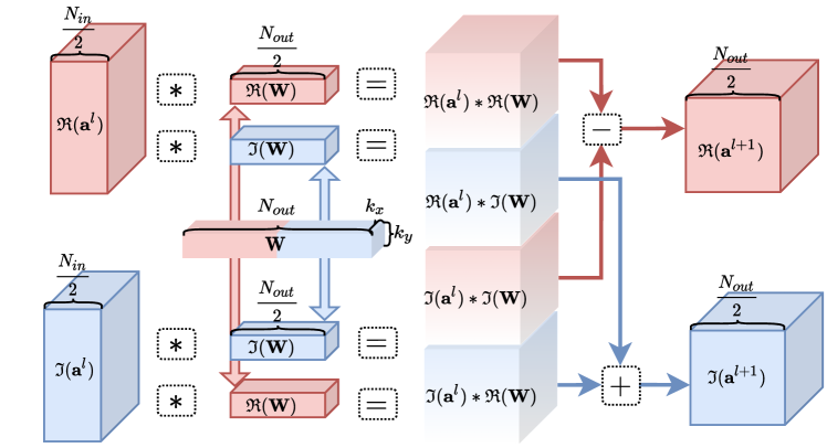
Figure 3: Depiction of a complex convolution on input $\mathbf{a}^{l}\in\mathbb{C}$ using the kernel $W\in\mathbb{C}$, creating the activation of the next level $\mathbf{a}^{l+1}\in\mathbb{C}$.

In complex analysis the multiplication of two complex numbers $z_{1}=(a+ib)$ and $z_{2}=(x+iy)$ results in $z_{1}\cdot z_{2}=ax-by+i(bx+ay)$, where $z_{1},z_{2}\in\mathbb{C}$ and $a,b\in\mathbb{R}$ with $i$ being the imaginary unit. The same works for complex tensors. Since the convolution operator ($*$) is distributive we obtain,

$$\small\mathbf{W}*\mathbf{h}=(\mathbf{A}+i\mathbf{B})*(\mathbf{x}+i\mathbf{y})=\mathbf{A}*\mathbf{x}-\mathbf{B}*\mathbf{y}+i(\mathbf{B}*\mathbf{x}+\mathbf{A}*\mathbf{y}),$$ (2)

convolving the complex vector $\mathbf{h}=\mathbf{x}+i\mathbf{y}$ with the complex kernel matrix $\mathbf{W}=\mathbf{A}+i\mathbf{B}$ [14]. Therefore, the complex-valued convolution can be executed as a series of real-valued convolutions, as shown in Fig. 3.

III-B Complex Batch Normalization

Deep CNNs rely on the Batch Normalization (BN) operation to normalize activations and accelerate training [21]. Since the standard formulation of BN only applies to real-valued activations, complex-valued networks require different methods. One possibility to realize BN for complex numbers was proposed in [14], where they use a whitening procedure to standardize the complex numbers. First the inputs $\mathbf{z}\in\mathbb{C}$ are whitened and then standard BN is performed. Thus, the vector after the whitening step is scaled and shifted using $\boldsymbol{\gamma}$ and $\boldsymbol{\beta}$ respectively.

$$\small\mathrm{BN}(\mathbf{z})=\boldsymbol{\gamma}\odot(\mathbf{V})^{-\frac{1}{2}}(\mathbf{z}-\mathbb{E}[\mathbf{z}])+\boldsymbol{\beta},$$ (3)

where $\mathbf{V}$ is a $2\times 2$ positive (semi)-definite covariance matrix. Since the proposed BN needs the square root of the inverse of $\mathbf{V}$, positive definiteness of the matrix is ensured by adding $\epsilon\mathbf{I}$ to $V$, which is known as Tikhonov regularization.

III-C Complex Rectified Linear Unit ($\mathbb{C}\mathrm{ReLU}$)

The complex-valued ReLU function is defined as

$$\small\mathbb{C}\mathrm{ReLU}(z)=\mathrm{ReLU}(\Re(z))+i\mathrm{ReLU}(\Im(z)).$$ (4)

Although it does not fulfil the Cauchy-Riemann equations everywhere and is therefore only holomorphic on a subset of $\mathbb{C}$, but it can be computed efficiently and experiments have shown superior performance compared to other proposed complex-valued activation functions [14].

IV CVCNN for range-Doppler processing

Our CVCNN takes RD-maps with interference as inputs and predicts denoised RD-maps as outputs.

IV-A Model

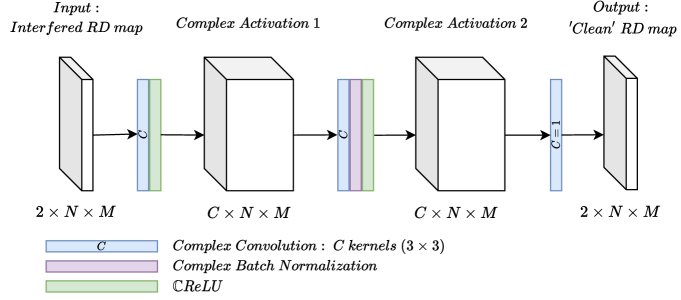
Figure 4: CVCNN architecture for radar signal denoising and interference mitigation. It uses $\mathbb{C}\mathrm{ReLU}$, complex BN and the complex-convolution.

The proposed CVCNN architecture for interference mitigation and denoising of radar signals is shown in Fig. 4 and based on the real-valued approach described in [22]. The CNN input is a noisy range-Doppler map, which is a complex-valued two dimensional matrix. This complex-valued matrix can be represented as a three dimensional tensor of size $C\times N\times M$ with $N$ and $M$ being the height and width of the RD-maps and $C=2$ the real- and imaginary parts of the complex spectra. The model architecture implements a fully convolutional NN; it consists exclusively of convolutions, BN operations and the ReLU activation function. The convolution strides are set to one and ’same’ zero padding is used such that the individual feature maps maintain a constant spatial size between layers. The CVCNN carries out all operations according to complex analysis as described in Section III. Therefore, three layers are constructed as follows:

1. The first layer performs a complex-convolution followed by a $\mathbb{C}\mathrm{ReLU}$ non-linearity.

2. In the second layer the complex-convolution is followed by a complex BN and a $\mathbb{C}\mathrm{ReLU}$ non-linearity.

3. The last layer consists solely of the convolution operation to create the network output.

IV-B Relation of computational and parameter complexity

Since CVCNNs have a higher computational complexity per-parameter, we present the number of mega (=million) floating point operations per RD-map (MFLOP/RD-map) over the number of parameters in Fig. 5. Note, that we consider the computational complexity per RD-sample for one prediction step of the network. As expected, we see that there is a linear relationship between the number of used filter channels and the computational complexity for both real-valued and complex-valued models. However, the linear relation of the complex-valued models has a larger slope than for the real-valued models. This means that a complex-valued model using the same number of parameters has a higher computational complexity than its real-valued counterpart.

Figure 5: Relation of the computational complexity and the number of model parameters. The labels of the networks indicate the number of filter channels in the corresponding layers.

V Experimental setup

We use real-world FMCW/CS radar measurements combined with simulated interference according to (1). The signals with and without interference are used as input-output pairs for training the CNN models in order to perform denoising and interference mitigation. The model is applied to the processed radar signal after the second DFT, i.e. the RD-map. We aim to correctly detect peaks in the RD-map that correspond to real objects rather than clutter or noise.

V-A Data set

The measurements were recorded in typical inner-city scenarios, where each measurement consists of 32 consecutive radar snapshots (RD-maps) each captured with sixteen antennas. The radar signal contains reflections from static and moving objects as well as receiver noise. The simulated interference, that is added to the time-domain measurement signal, is generated by sampling uniformly from the ego radar and interferer radar transmit parameters. See [22] for a detailed description of the simulation parameters and [8, 23] for an extensive analysis of the used measurement signals.

V-B Evaluation metrics

The models are evaluated using the F1-Score, Error Vector Magnitude (EVM) and Peak Phase Mean Squared Error (PPMSE), defined as follows:

V-B1 F1-Score

The F1-Score is a combined classification measure including the true-positive $t_{p}$, false-positive $f_{p}$ and false-negative $f_{n}$ object detections. It is defined as

$$\small F_{1}=2\cdot\dfrac{t_{p}}{t_{p}+\frac{1}{2}(f_{p}+f_{n})}.$$ (5)

For the F1-Score calculation, we first use the Cell Averaging - Constant False Alarm Rate (CA-CFAR) peak detector on the RD-map prediction $S_{\mathrm{RD}}[n,m]$ in order to create a binary object detection map. This object detection map forms, in combination with the ground truth object detection map, the basis for calculating $t_{p}$, $f_{p}$ and $f_{n}$.

V-B2 Error Vector Magnitude (EVM)

The EVM measures the deviation of the predicted RD-map $S_{\mathrm{RD}}[n,m]$ from the clean RD-map $S_{\mathrm{RD,clean}}[n,m]$ at ground truth peak locations. It it given as

$$\small\mathrm{EVM}=\frac{1}{N_{\mathrm{O}}}\sum_{\{n,m\}\in\mathcal{O}}\dfrac{|S_{\mathrm{RD,clean}}[n,m]-S_{\mathrm{RD}}[n,m]|}{|S_{\mathrm{RD,clean}}[n,m]|},$$ (6)

where $n$ and $m$ are the indices of the object, within the set of cells $\mathcal{O}$, containing object peaks, and $N_{\mathrm{O}}$ is the number of detected peaks.

V-B3 Peak Phase Mean Squared Error (PPMSE)

The PPMSE measures the average squared difference between the angle of the clean range-Doppler signal vector $S_{\mathrm{RD,clean}}[n,m]$ and the predicted range-Doppler signal vector $S_{\mathrm{RD}}[n,m]$ of all detected object peaks. It is defined as

$$\small\begin{split}&\Delta[n,m]=\left\lvert\mathrm{atan2}\left(\frac{\Im(S_{\mathrm{RD}}[n,m])}{\Re(S_{\mathrm{RD}}[n,m])}\right)-\mathrm{atan2}\left(\frac{\Im(S_{\mathrm{RD,clean}}[n,m])}{\Re(S_{\mathrm{RD,clean}}[n,m])}\right)\right\rvert,\\ &\mathrm{PPMSE}[n,m]=\frac{1}{N_{\mathrm{O}}}\sum_{\{n,m\}\in\mathcal{O}}\min(\Delta[n,m],2\pi-\Delta[n,m])^{2},\end{split}$$ (7)

where $n$ and $m$ are the indices of cells containing object peaks $\mathcal{O}$ and $N_{\mathrm{O}}$ is the number of detected peaks.

V-C Training settings

The interfered RD-maps $S_{\mathrm{RD,interfered}}$ are used as inputs for the CNN, while the clean RD-maps $S_{\mathrm{RD,clean}}$ are used as the training targets. All RD-maps are cropped to $N\times M=96\ \textrm{range cells}\times 96\ \textrm{Doppler cells}$ and subsequently scaled to zero-mean and unit-variance. The models were trained for 100 epochs using Adam [24] with a learning rate of $5\cdot 10^{-3}$ and a mini-batch size of $L=8$. As our training objective, we use the mean squared error (MSE) of real- and imaginary parts of the predictions $S_{\mathrm{RD}}$ and targets $S_{\mathrm{RD,clean}}$

VI Experiments

We evaluate the denoising capabilities of CVCNNs for RD-maps with simulated interference. We compare complex-valued networks with their real-valued equivalent evaluating the computational, parameter and data efficiency. Furthermore, we analyze the performance of both CNN approaches against classical methods.

VI-A Parameter efficiency

In this experiments we investigate the parameter efficiency of CVCNNs compared to their real-valued counterparts. Therefore, we train and evaluate 24 different architectures varying the number of filter channels $C_{i}$ per layer $i$. For the complex-valued network we vary the number of (complex-valued) filter kernels (= channels in the next activation map) in the first layer using $C_{1}\in\{1,2,4,8,16,32\}$ kernels and in the second layer using $C_{2}\in\{2,4,8,16\}$ kernels. The output layer is fixed to $C_{3}=1$ complex-valued filter kernel. The real-valued network uses $C_{1}\in\{1,2,4,8,16,32\}$, $C_{2}\in\{4,8,16,32\}$ and $C_{3}=2$ real-valued filter kernels. We combine the sets of kernels per layer as a Cartesian product and thus evaluate all possible combinations, yielding 24 architectures for each approach.

Figure 6: Parameter efficiency of RVCNNs and CVCNNs. F1-Score and EVM over the number of parameters were used as performance metrics. The best real-valued and complex-valued models are annotated with their number of parameters.

The results in Fig. 6 show, that the complex-valued networks outperform the real-valued networks with respect to performance per parameter count. All metrics show substantial improvements across all architecture combinations. Complex-valued network architectures below 500 parameters can deliver comparable performance to even the largest used real-valued networks, reducing the overall memory footprint of the network.

VI-B Computational efficiency

Parameter efficiency does not directly translate to computational efficiency, since complex-valued operations are slightly more computationally demanding than real-valued operations as discussed in Section IV-B. Therefore, the same architectures as above were used in order to evaluate the performance of the models w.r.t their computational efficiency in MFLOP/RD-map. Note, that we consider the computational complexity per RD-sample for one prediction step of the network.

Figure 7: Computational efficiency in MFLOP/RD-map of RVCNNs and CVCNNs. F1-Score and EVM over MFLOP/RD-map were used as performance metrics. The best real-valued and complex-valued models are annotated with the used MFLOPS/RD-map.

Comparing the results of the complex-valued network in Fig. 7 with Fig. 6, we see that the improvement in performance compared to the real-valued networks is not as pronounced as in the last experiment. This means that while being very parameter efficient, the complex-valued models introduce a lot of computational overhead. Therefore, the performance improvement on a per FLOP level is smaller than for the case of only considering parameter count. Nevertheless, the complex-valued models are able to outperform their real-valued counterparts for most architectures.

VI-C Data efficiency

In this experiments we vary the used training data with a step size of one percent. The total number of training samples (=RD-maps) is 2500, which gives a minimum number and step size of 25 training samples. We compare a three layer real-valued network containing 16-8-2 channels ($\mathbb{R}$ 16-8-2) with two variants of complex-valued networks ($\mathbb{C}$ 8-8-1 and $\mathbb{C}$ 8-4-1). The two complex-valued network variants are selected, such that they have a similar number of real-valued parameters (i.e. $\mathbb{C}$ 8-8-1) and a similar computational complexity (i.e. $\mathbb{C}$ 8-4-1) when compared to the real-valued baseline. See Section IV-B and in particular Fig. 5 for details about the parameter-to-FLOP/RD-map relation of real-valued and complex-valued networks. The figure indicates the closest complex-valued architectures with respect to both considered complexity measures, i.e. parameters and FLOP/RD-map.

Figure 8: Data efficiency of a real-valued ($\mathbb{R}$ 16-8-2) and a complex-valued network ($\mathbb{C}$ 8-4-1) with similar computational complexity. The F1-Score and EVM have been evaluated using different percentages (1% to 100%) of the training data.

TABLE I contains the F1-Score, EVM and PPMSE results for the two chosen network architectures ($\mathbb{C}$ 8-4-1 and $\mathbb{C}$ 8-8-1 complex channels) and the real-valued baseline model ($\mathbb{R}$ 16-8-2) for different fractions of used training data. Both complex-valued network architectures clearly outperform the real-valued equivalent, while the bigger complex-valued model $\mathbb{C}$ 8-8-1 typically yields the best performance scores. Fig. 8 illustrates the data efficiency analysis of the smaller CVCNN architecture ($\mathbb{C}$ 8-4-1) and the real-valued baseline.

In general, the more training data we use, the better is the test performance for all three metrics (F1-Score, EVM and PPMSE). However, complex-valued networks require much less training samples in order to yield high performances. While a complex-valued network reaches almost top results with only 10% of the training samples, a comparable real-valued network requires at least 50% of the training samples in order to train robustly and reach high performances. The performance difference is particularly high for metrics that consider phase information (EVM and PPMSE). This emphasizes the need for an accurate treatment of complex input domains in order to correctly infer complex information.

Metric	Model	Used data
		20 %	40 %	60 %	80 %	100 %
F1-Score	$\mathbb{C}$ 8-8-1	0.895	0.898	0.896	0.898	0.897
	$\mathbb{C}$ 8-4-1	0.897	0.896	0.897	0.896	0.897
	$\mathbb{R}$ 16-8-2	0.872	0.881	0.887	0.891	0.885
EVM	$\mathbb{C}$ 8-8-1	0.163	0.136	0.124	0.117	0.115
	$\mathbb{C}$ 8-4-1	0.163	0.143	0.133	0.127	0.122
	$\mathbb{R}$ 16-8-2	0.258	0.262	0.209	0.184	0.146
PPMSE / $\mathbf{rad^{2}}$	$\mathbb{C}$ 8-8-1	0.017	0.014	0.013	0.013	0.013
	$\mathbb{C}$ 8-4-1	0.018	0.016	0.015	0.014	0.014
	$\mathbb{R}$ 16-8-2	0.049	0.054	0.035	0.022	0.018

TABLE I: F1-Score, EVM and PPMSE results for different fractions of used training data. The RVCNN ($\mathbb{R}$ 16-8-2 channels) is compared to two CVCNNs ($\mathbb{C}$ 8-8-1 and $\mathbb{C}$ 8-4-1). The F1-Score without mitigation and from the target measurements is $\mathrm{F_{NoMit.}}=0.837$ and $\mathrm{F_{Target}}=0.909$, respectively.

VI-D Comparison with classical signal processing methods

We compare our best CNN-based models in the real-valued setting ($\mathbb{R}$-model) as well as in the complex-valued setting ($\mathbb{C}$-model) with the classical and state-of-the-art interference mitigation methods zeroing [1], Iterative method with adaptive thresholding (IMAT) [25] and Ramp filtering [2]; see [26] for an overview of these methods. Zeroing and IMAT highly depend on an interference detection step, which influences their performance considerably. In our experiments we identified time-domain samples incorporating interference with approximately 90% accuracy; this interference detection rate seems feasible in practice. Note that Ramp filtering as well as the CNN-based models do not depend on such an explicit interference detection step. The average results for all methods are given in TABLE II. Fig. 9 shows the empirical cumulative density function (CDF) using the per-sample F1-Score and the EVM at peak locations. The ’clean’ measurement and interfered signals are included as reference. All classical methods, namely zeroing, IMAT and Ramp filtering, improve the F1-Score (as shown in Fig. 9(a)) when applied to the measurement signal with interference. Zeroing and IMAT yield very similar F1-Scores. Ramp filtering outperforms both other classical methods, particularly for samples with strong interference (see black magnification).

The CNN-based models, both with real-valued as well as complex-valued weights and activations, are competitive with the classical methods for all considered interference levels and even outperform the best classical method, namely Ramp filtering (see black magnification). The CDF shape indicates that the CNN-based models are robust with respect to different interference patterns and levels. This is indicated by the CDF’s narrow form and high values for the lowest F1-Scores per CNN model (see gray magnification). Note, that the F1-Score, and thus the detection sensitivity, of both CNN-based models is very close to the theoretical maximum, namely the CDF of the clean data.

Fig. 9(b) shows the empirical CDF of the EVM. Generally, the better the mitigation in terms of F1-Score, the higher is the EVM and thus the distortion of the phase at object peaks. In comparison to the RVCNN, the CVCNN reduces the peak distortions although it achieves a very similar F1-Score and it even outperforms the best classical method in terms of EVM, namely IMAT. Hence, the CVCNN achieves very high F1-Scores while also retaining low EVMs. The PPMSE in Fig. 9(c) shows similar characteristics. The CVCNN outperforms all other methods incorporating less phase distortions, particularly for weak interferences.

	F1-Score	EVM	PPMSE	Params	MFLOP
$\mathbb{R}$-16-16-2*	0.896	0.123	0.015	2946	53.24
$\mathbb{C}$-32-16-1*	0.902	0.098	0.011	10242	374.27
Zeroing	0.856	0.124	0.069	-	2.83
RFmin	0.875	0.145	0.054	-	3.13
IMAT	0.860	0.119	0.065	-	3.88

TABLE II: Performance comparison of real- and complex-valued models^* with the three classical methods zeroing, IMAT and Ramp filtering in terms of F1-Score, EVM and PPMSE. The F1-Score without mitigation and from the target measurements is $\mathrm{F_{NoMit.}}=0.837$ and $\mathrm{F_{Target}}=0.909$, respectively. *Model selected based on the best EVM result in the design space.

(a) CDF of the samplewise F1-Score

(b) CDF of the samplewise EVM

(c) CDF of the samplewise PPMSE in $rad^{2}$

Figure 9: Empirical CDF performance comparison between the real-valued model^* ($\mathbb{R}$-model), the complex-valued model^* ($\mathbb{C}$-model), and the three classical methods zeroing, IMAT and Ramp filtering. *Model selected based on the best EVM result in the design space.

VII Conclusion

We propose the use of complex-valued CNNs for range-Doppler denoising and interference mitigation of automotive radar signals. The proposed NN architecture follows complex-valued analysis and thus processes the complex-valued signals according to their physical characteristics. This inductive bias restricts the network structure and operations in a meaningful way and therefore reduces the complexity of the learning problem. We confirm this claim with experiments on complex-valued radar signals. We show, that complex-valued networks with a similar (1) number of parameters and (2) computational complexity substantially improve all considered metrics (F1-Score, EVM and PPMSE) and that they are able to operate on much smaller training sets. Particularly the high performance of metrics considering the phase information (EVM and PPMSE) reveals the advantage of complex-valued NNs for applications on complex-valued signal domains. The proposed approach might thus be crucial for processing complex-valued signals, such as automotive radar signals containing valuable phase information, e.g. for angle estimation. In future research we want to focus on the transferability of models between different radar antennas, the impact of multi-antenna information during training and the direct evaluation of angle estimation capabilities.

References

- [1] C. Fischer, Untersuchungen zum Interferenzverhalten automobiler Radarsensorik. PhD thesis, Ulm University, 2016.
- [2] M. Wagner, F. Sulejmani, A. Melzer, P. Meissner, and M. Huemer, “Threshold-Free Interference Cancellation Method for Automotive FMCW Radar Systems,” in 2018 IEEE Int. Symposium on Circuits and Systems (ISCAS), 2018.
- [3] F. Marvasti, M. Azghani, P. Imani, P. Pakrouh, S. Heydari, A. Golmohammadi, A. Kazerouni, and M. Khalili, “Sparse signal processing using iterative method with adaptive thresholding (IMAT),” in 2012 19th Int. Conf. on Telecommunications (ICT), 2012.
- [4] J. Bechter, K. D. Biswas, and C. Waldschmidt, “Estimation and cancellation of interferences in automotive radar signals,” in 2017 18th Int. Radar Symposium (IRS), pp. 1–10, 2017.
- [5] J. Bechter, K. Eid, F. Roos, and C. Waldschmidt, “Digital beamforming to mitigate automotive radar interference,” 2016 IEEE MTT-S Int. Conf. Microwaves Intell. Mobility, ICMIM 2016, pp. 2–5, 2016.
- [6] J. Mun, H. Kim, and J. Lee, “A deep learning approach for automotive radar interference mitigation,” in 2018 IEEE 88th Vehicular Technology Conf. (VTC-Fall), pp. 1–5, 2018.
- [7] J. Mun, S. Ha, and J. Lee, “Automotive radar signal interference mitigation using RNN with self attention,” in ICASSP 2020 - 2020 IEEE Int. Conf. on Acoustics, Speech and Signal Processing (ICASSP), pp. 3802–3806, 2020.
- [8] J. Rock, M. Toth, P. Meissner, and F. Pernkopf, “Deep interference mitigation and denoising of real-world fmcw radar signals,” in 2020 IEEE Int. Radar Conf. (RADAR), pp. 624–629, 2020.
- [9] J. Rock, W. Roth, M. Toth, P. Meissner, and F. Pernkopf, “Resource-efficient deep neural networks for automotive radar interference mitigation,” IEEE Journal of Selected Topics in Signal Processing, 2021. Accepted for publication.
- [10] M. L. L. de Oliveira and M. J. G. Bekooij, “Deep convolutional autoencoder applied for noise reduction in range-doppler maps of fmcw radars,” in 2020 IEEE Int. Radar Conf. (RADAR), pp. 630–635, 2020.
- [11] J. Fuchs, A. Dubey, M. Lübke, R. Weigel, and F. Lurz, “Automotive radar interference mitigation using a convolutional autoencoder,” in 2020 IEEE Int. Radar Conf. (RADAR), pp. 315–320, 2020.
- [12] N.-C. Ristea, A. Anghel, and R. T. Ionescu, “Fully Convolutional Neural Networks for Automotive Radar Interference Mitigation,” 7 2020.
- [13] G. M. Georgiou and C. Koutsougeras, “Complex domain backpropagation,” IEEE transactions on Circuits and systems II: analog and digital signal processing, vol. 39, no. 5, pp. 330–334, 1992.
- [14] C. Trabelsi, O. Bilaniuk, D. Serdyuk, S. Subramanian, J. F. Santos, S. Mehri, N. Rostamzadeh, Y. Bengio, and C. J. Pal, “Deep complex networks,” CoRR, vol. abs/1705.09792, 2017.
- [15] Z. Zhang, H. Wang, F. Xu, and Y. Jin, “Complex-valued convolutional neural network and its application in polarimetric sar image classification,” IEEE Transactions on Geoscience and Remote Sensing, vol. 55, no. 12, pp. 7177–7188, 2017.
- [16] J. Gao, B. Deng, Y. Qin, H. Wang, and X. Li, “Enhanced radar imaging using a complex-valued convolutional neural network,” IEEE Geoscience and Remote Sensing Letters, vol. 16, no. 1, pp. 35–39, 2019.
- [17] A. G. Stove, “Linear FMCW radar techniques,” IEE Proceedings F - Radar and Signal Processing, vol. 139, no. 5, pp. 343–350, 1992.
- [18] V. Winkler, “Range Doppler detection for automotive FMCW radars,” in 2007 European Microwave Conf., pp. 1445–1448, Oct. 2007.
- [19] M. Toth, P. Meissner, A. Melzer, and K. Witrisal, “Analytical Investigation of Non-Coherent Mutual FMCW Radar Interference,” in 2018 European Radar Conf. (EURAD), pp. 71–74, 2018.
- [20] A. Hirose, Complex-valued neural networks, vol. 400. Springer Science & Business Media, 2012.
- [21] S. Ioffe and C. Szegedy, “Batch normalization: Accelerating deep network training by reducing internal covariate shift,” CoRR, vol. abs/1502.03167, 2015.
- [22] J. Rock, M. Toth, E. Messner, P. Meissner, and F. Pernkopf, “Complex signal denoising and interference mitigation for automotive radar using convolutional neural networks,” in 2019 22nd Int. Conf. on Information Fusion (FUSION) (FUSION 2019), 2019.
- [23] M. Toth, J. Rock, P. Meissner, A. Melzer, and K. Witrisal, “Analysis of automotive radar interference mitigation for real-world environments,” in European Radar Conf. (EURAD), 2020. Accepted for publication.
- [24] D. P. Kingma and J. Ba, “Adam: A method for stochastic optimization,” CoRR, vol. abs/1412.6980, 2014.
- [25] J. Bechter, F. Roos, M. Rahman, and C. Waldschmidt, “Automotive Radar Interference Mitigation Using a Sparse Sampling Approach,” in 2017 European Radar Conf. (EURAD), pp. 90–93, 2017.
- [26] S.-W. Fu, T.-y. Hu, Y. Tsao, and X. Lu, “Complex spectrogram enhancement by convolutional neural network with multi-metrics learning,” in 2017 IEEE 27th Int. Workshop on Machine Learning for Signal Processing (MLSP), pp. 1–6, IEEE, 2017.