Dynamic phase transition of charged dilaton black holes

Abstract

Dynamic phase transition of charged dilaton black holes is investigated in this paper. We introduce the Gibbs free energy landscape and calculate the corresponding $G_{L}$ for the dilaton black hole. On the one hand, we numerically solve the Fokker-Planck equation constrained by only the reflecting boundary condition. The effects of dilaton gravity on the probabilistic evolution of dilaton black holes are quite obvious. Firstly, the horizon radius difference between the large dilaton black hole and small dilaton black hole increases with the parameter $\alpha$. Secondly, with the increasing of $\alpha$, the system needs much more time to achieve a stationary distribution. Thirdly, the value which $\rho(r_{l},t)$ and $\rho(r_{s},t)$ finally attain varies with the parameter $\alpha$. On the other hand, resolving Fokker-Planck equation constrained by both the reflecting boundary condition and absorbing boundary condition, we investigate the first passage process of dilaton black holes. The initial peak decays more slowly with the increase of $\alpha$, which can also be witnessed from the slow down of the decay of $\Sigma(t)$ (the sum of the probability that the black hole system having not finished a first passage by time $t$). Moreover, the time corresponding to the single peak of the first passage time distribution is also found to increase with the parameter $\alpha$. Considering all the observations mentioned above, the dilaton field does slow down the dynamic phase transition process between the large black hole and small black hole.

I Introduction

Dilaton gravity Gibbons1 ; Garfinkle ; Koikawa has received considerable attention within the community for its great physical significance. Firstly, it serves as the low energy limit of string theory. One can recover Einstein gravity with a non-minimally coupled dilaton field and other fields in the low energy limit. Secondly, there exist one or more Liouville-type potentials in its action. And these potentials can be caused by spacetime supersymmetry breaking in ten dimensions. Thirdly, it has been disclosed that the dilaton field may affect both the casual structure and thermodynamic properties of black holes. Due to the above physical importance, various black hole solutions were presented with their thermodynamic properties discussed Gibbons1 - zhangchengyong . Interestingly, it was argued in Refs. gaochangjun1 ; gaochangjun2 ; gaochangjun3 that the cosmological constant is found to be coupled to Liouville-type potential in the dilaton theory.

Among these solutions, a class of $(n+1)$-dimensional topological black hole solutions were obtained Sheykhi2 in Einstein-Maxwell-dilaton theory, which are neither asymptotically flat nor anti-de Sitter. Thermodynamic properties of these black holes were carefully analyzed. Moreover, the effect of dilaton field on thermal stability was disclosed Sheykhi2 . $P-V$ criticality was investigated in Refs. zhaoren ; Sheykhi1 . Provided the coupling constant of dilaton gravity is less than one, the critical values of relevant physical quantities are physical Sheykhi1 . Ref. Sheykhi13 probed the phase transition and thermodynamic geometry while Ref. Sheykhi16 further disclosed the existence of zeroth-order phase transition. Both the two point correlation function and the entanglement entropy of dilaton black holes were studied by one of us xiong10 , providing an alternative perspective to observe the critical phenomena in dilaton black holes. With the tool of Ruppeiner geometry, Ref. zhangshaojun tried to provide the microscopic explanation for phase transitions of charged dilatonic black holes.

Although many attempts have been made as stated above, the dynamical phase transition of this typical class of dilaton black hole solution proposed in Ref. Sheykhi2 and the possible kinetics behind it remains to be probed. So it is the main motivation of this paper to complete this “missing puzzle piece” concerning the phase transition of charged dilaton black holes. Dynamic phase transition of black holes has been a newly emerged hot topic ever since the creative works reporting the kinetics of the Hawing-Page phase transition liran1 and the van der Waals like phase transition liran2 recently. For the latter, the transition between the large black hole and the small black hole due to thermal fluctuation can be viewed as stochastic process, which can be probed via the tool of Fokker-Planck equation liran2 . Soon after, dynamic phase transition of Gauss-Bonnet black holes liran3 ; weishaowen2 ; weishaowen3 and charged AdS black holes surrounded by quinteness dark energy xiong11 were investigated. More interestingly, it was even suggested in a very recent work liran4 that the turnover of the kinetics can be used to probe the microstructure of black holes. It is certainly of interest to generalize these pioneer works to dilaton black holes considering the great physical importance of dilaton gravity stated in the first paragraph of this paper. It is expected that novel features will be disclosed about the dynamic phase transition of black holes.

The organization of this paper is as follows. Sec.II is devoted to a short review of thermodynamic properties of charged dilaton black holes. In Sec.III, we will investigate the dynamic phase transition of charged dilaton black holes. We will further probe the first passage process for the phase transition of charged dilaton black holes in Sec.IV. Conclusions will be presented in Sec.V.

II A short review on thermodynamic properties of charged dilaton black holes

The Einstein-Maxwell-Dilaton action in $(n+1)$-dimensional spacetime reads Chan

$$S=\frac{1}{16\pi}\int d^{n+1}x\sqrt{-g}\left(\mathcal{R}-\frac{4}{n-1}(\nabla\Phi)^{2}-V(\Phi)-(e^{-4\alpha\Phi/(n-1)}F_{\mu\nu}F^{\mu\nu}\right),\\$$ (1)

where $\mathcal{R}$, $\Phi$ and $F_{\mu\nu}$ denote respectively the Ricci scalar curvature, the dilaton field and the electromagnetic field tensor. The parameter $\alpha$ describes the strength of coupling between the electromagnetic field and the dilaton field.

To obtain a solution, one needs to take a specific form for the potential of the dilaton field $V(\Phi)$. Here, the potential of the dilaton field is chosen as $V(\Phi)=2\Lambda_{0}e^{2\zeta_{0}\Phi}+2\Lambda e^{2\zeta\Phi}$ Chan ; Sheykhi4 ; Sheykhi2 ; Sheykhi3 . Note that if one consider the power-law Maxwell field Sheykhi8 , an additional term should be added to the potential mentioned above.

One can take the general form of metric as Sheykhi2

$$ds^{2}=-f(r)dt^{2}+\frac{1}{f(r)}dr^{2}+r^{2}R^{2}(r)h_{ij}dx^{i}dx^{j},\\$$ (2)

where $h_{ij}dx^{i}dx^{j}$ corresponds to $(n-1)$-dimensional hypersurface with constant scalar curvature $(n-1)(n-2)k$. $k$ can be taken as $-1,\,0,\,1$, corresponding to hyperbolic, flat and spherical constant curvature hypersurface respectively.

Making the ansatz $R=e^{2\alpha\Phi/(n-1)}$, the corresponding solution was derived Sheykhi2 as

$$f(r) = -\frac{k(n-2)(1+\alpha^{2})^{2}b^{-2\gamma}r^{2\gamma}}{(\alpha^{2}-1)(\alpha^{2}+n-2)}-\frac{m}{r^{(n-1)(1-\gamma)-1}}+\frac{2\Lambda b^{2\gamma}(1+\alpha^{2})^{2}r^{2(1-\gamma)}}{(n-1)(\alpha^{2}-n)}$$ (3)

$$+\frac{2q^{2}(1+\alpha^{2})^{2}b^{-2(n-2)\gamma}r^{2(n-2)(\gamma-1)}}{(n-1)(n+\alpha^{2}-2)},$$

$$\Phi(r) = \frac{(n-1)\alpha}{2(\alpha^{2}+1)}\ln\left(\frac{b}{r}\right),$$ (4)

where $b$ is an arbitrary constant and $\gamma$ is related to $\alpha$ by $\gamma=\alpha^{2}/(\alpha^{2}+1)$. And the coefficients in the expression of $V(\Phi)$ read Sheykhi2

$$\Lambda_{0}=\frac{k(n-1)(n-2)\alpha^{2}}{2b^{2}(\alpha^{2}-1)},\;\zeta_{0}=\frac{2}{\alpha(n-1)},\;\zeta=\frac{2\alpha}{n-1}.\\$$ (5)

The mass, the charge, Hawking temperature and the entropy was obtained respectively as Sheykhi2 ; zhaoren

$$M = \frac{b^{(n-1)\gamma}(n-1)\omega_{n-1}m}{16\pi(\alpha^{2}+1)},$$ (6)

$$Q = \frac{\omega_{n-1}q}{4\pi},$$ (7)

$$T = \frac{-(1+\alpha^{2})}{2\pi(n-1)}\Big{[}\frac{k(n-2)(n-1)}{2b^{2\gamma}(\alpha^{2}-1)}r_{+}^{2\gamma-1}+\Lambda b^{2\gamma}r_{+}^{1-2\gamma}+q^{2}b^{-2(n-2)\gamma}r_{+}^{(2n-3)(\gamma-1)-\gamma}\Big{]},$$ (8)

$$S = \frac{\omega_{n-1}b^{(n-1)\gamma}r_{+}^{(n-1)(1-\gamma)}}{4}.$$ (9)

where the parameter $m$ can be derived via $f(r_{+})=0$.

Considering the demand that the electric potential $A_{t}$ should be finite at infinity and the parameter $m$ should vanish at spacial infinity, restrictions on $\alpha$ for dilaton black holes coupled with power-law Maxwell field was obtained Sheykhi8 as $0\leq\alpha^{2}<n-2$ for the case $\frac{1}{2}<p<\frac{n}{2}$ while $2p-n<\alpha^{2}<n-2$ for the case $\frac{n}{2}<p<n-1$, where $p$ describes the nonlinearity of the electromagnetic field. For the Maxwell field here, $p=1$. And the corresponding restriction reduces to be $0\leq\alpha^{2}<n-2$.

III Dynamic phase transition of charged dilaton black holes

To probe the dynamic phase transition of black holes, one should introduce the “Gibbs free energy landscape” and define the corresponding Gibbs free energy $G_{L}$ as $G_{L}=H-T_{E}S$. Here, $T_{E}$ denotes the temperature of the ensemble. As suggested in the pioneer work liran1 ; liran2 ; weishaowen2 , $G_{L}$ possesses the following properties. Firstly, only when $T_{E}=T$, $G_{L}$ describes a real black hole. Secondly, only the extremal points of $G_{L}$ make sense. The local maximum and minimum denote respectively the unstable and stable black hole phases. Thirdly, the small-large black hole phase transition corresponds to the double wells of $G_{L}$ having the same depth.

Via Eqs. (6) and (9), $G_{L}$ of the dilaton black hole can be calculated as

$$G_{L} = \frac{\omega_{n-1}b^{(n-1)\gamma}r_{+}^{n-2+(1-n)\gamma}}{16\pi}\Big{\{}\Big{[}\frac{2b^{-2(n-2)\gamma}q^{2}r_{+}^{2(n-2)(\gamma-1)}}{(n-1)(\alpha^{2}+n-2)}-\frac{k(n-2)b^{-2\gamma}r^{2\gamma}}{(\alpha^{2}-1)(\alpha^{2}+n-2)}+\frac{16\pi Pb^{2\gamma}r^{2(1-\gamma)}}{(n-1)(n-\alpha^{2})}\Big{]}$$ (10)

$$\times(n-1)(1+\alpha^{2})-4\pi r_{+}T_{E}\Big{\}},$$

where we have introduced the extended phase space and identify the thermodynamic pressure as $P=-\Lambda/8\pi$.

Based on $G_{L}$, we can utilize the following Fokker-Planck equation Zwanzig ; Lee1 ; Lee2 ; wang1 ; Bryngelson to investigate the probabilistic evolution of the black hole after the thermal fluctuation

$$\frac{\partial\rho(r,t)}{\partial t}=D\frac{\partial}{\partial r}\left\{e^{-\beta G_{L}(T,P,r)}\frac{\partial}{\partial r}\left[e^{\beta G_{L}(T,P,r)}\rho(r,t)\right]\right\},$$ (11)

where $\rho(r,t)$ denotes the probability distribution. The parameter $\beta=\frac{1}{k_{B}T}$ with $k_{B}$ as the Boltzman constant. The diffusion coefficient $D=\frac{k_{B}T}{\zeta}$ with $\zeta$ denoting the dissipation coefficient. Without loss of generality, one can set $\zeta$ and $k_{B}$ as one. For the sake of conciseness, we use the notation $r$ to replace the notation $r_{+}$ for the black hole horizon radius here and hereafter.

Before solving the above equation, one should impose both the boundary condition and the initial condition first. The boundary conditions can be divided into two categories, reflecting boundary condition and absorbing boundary condition. As suggested in Ref. liran2 , the reflecting boundary condition can be considered as $\beta G^{\prime}(r)\rho(r,t)+\rho^{\prime}(r,t)\big{|}_{r=r_{0}}=0$ while absorbing boundary condition can be considered as $\rho(r_{m},t)=0$ (The meaning of $r_{m}$ would be discussed in the next paragraph). The initial condition can be chosen as Gaussian wave pocket located at the small/large dilaton black hole state respectively. Namely, $\rho(r,0)=\frac{1}{\sqrt{\pi}a}e^{-(r-r_{l(s)})^{2}/a^{2}}$, with $r_{l}$ and $r_{s}$ denote the horizon radius of large dilaton black hole and small dilaton black hole respectively liran2 .

We numerically solve Eq.(11) constrained by both the initial condition and the reflecting boundary condition mentioned above. Fig.1 shows the time evolution of the probability distribution $\rho(r,t)$ of charged dilaton AdS black holes, where the thermodynamic pressure is chosen as $P=0.003$. In the top, middle and bottom rows of Fig.1, the parameter characterizing the strength of coupling between the electromagnetic field and the dilaton field $\alpha$ is chosen to be $0.4,0.2,0$ respectively to compare the effect of dilaon gravity on the probability evolution.

For the left three graphs of Fig.1, the initial condition is chosen as Gaussian wave pocket located at the large dilaton black hole state. This can be reflected in the graphs that the initial peak of $\rho(r,t)$ corresponds to the radius of the large dilaton black hole. With the time evolution, the initial peak is decreasing while another peak corresponds to the radius of the small dilaton black hole is booming. Finally, these two peaks reach a stationary distribution that they equal to each other at the first sight. This clearly exhibits the dynamic process of how the initial large dilaton black hole evolves into the small dilaton black hole. So the left three graphs correspond to the case the large dilaton black hole evolves dynamically into small dilaton black hole.

By contrast, the initial condition is chosen as Gaussian wave pocket located at the small dilaton black hole state for the right three graphs of Fig.1. The initial peak locating at the small dilaton black hole is decaying while another peak corresponding to the radius of the large dilaton black hole is increasing with the time evolution. At the long time limit, these two peaks corresponding to the large (small) black holes respectively approach to a stationary distribution. So the right three graphs of Fig.1 correspond to the case the small dilaton black hole evolves dynamically into large dilaton black hole.

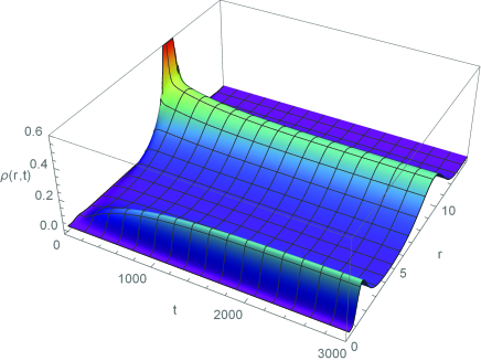
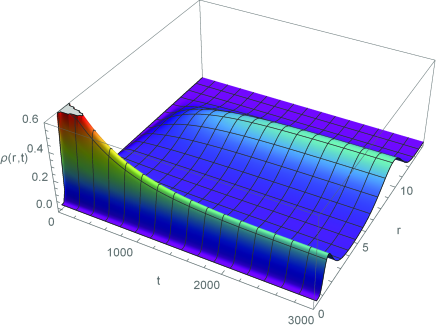
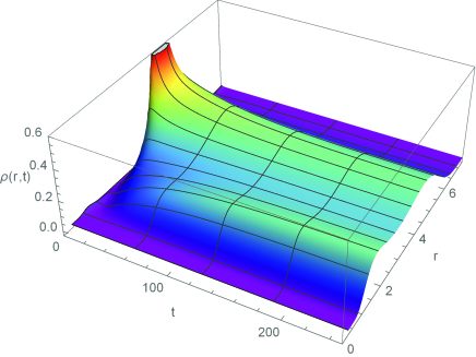
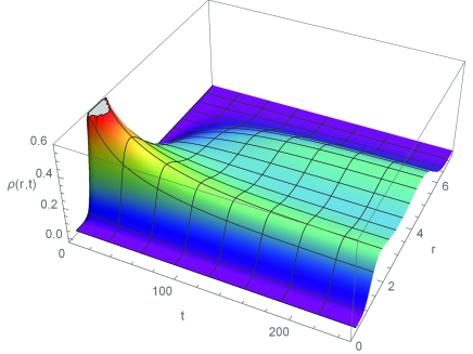
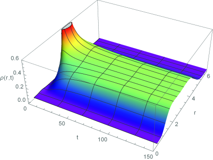
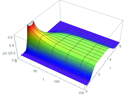
Figure 1: Time evolution of $\rho(r,t)$ for charged dilaton black hole with $b=1,q=1,P=0.003$. (a) $\alpha=0.4$ (b) $\alpha=0.4$ (c) $\alpha=0.2$ (d) $\alpha=0.2$ (e) $\alpha=0$ (f) $\alpha=0$. For the left three graphs, the initial condition is chosen as Gaussian wave pocket located at the large dilaton black hole state while for the right three graphs, the initial condition is chosen as Gaussian wave pocket located at the small dilaton black hole state.

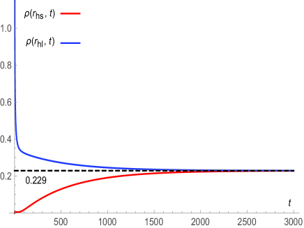
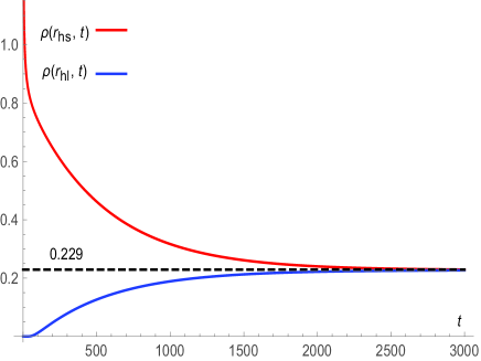
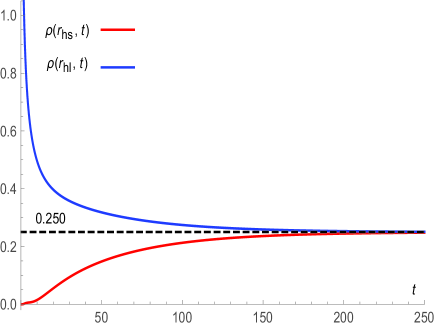
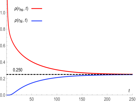
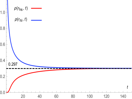
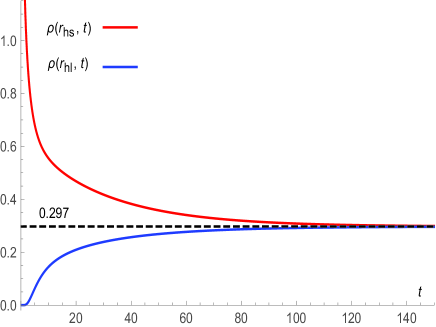
Figure 2: Time evolution of $\rho(r_{l},t)$ and $\rho(r_{s},t)$ for charged dilaton black hole with $b=1,q=1,P=0.003$. (a) $\alpha=0.4$ (b) $\alpha=0.4$ (c) $\alpha=0.2$ (d) $\alpha=0.2$ (e) $\alpha=0$ (f) $\alpha=0$. For the left three graphs, the initial condition is chosen as Gaussian wave pocket located at the large dilaton black hole state while for the right three graphs, the initial condition is chosen as Gaussian wave pocket located at the small dilaton black hole state.

Comparing the top two graphs ($\alpha=0.4$), the middle two graphs ($\alpha=0.2$) with the bottom two graphs ($\alpha=0$) in Fig.1, the effect of dilaton gravity is quite obvious. Firstly, the horizon radius difference between the large dilaton black hole and small dilaton black hole increases with the parameter $\alpha$. Secondly, with the increasing of $\alpha$, the system needs much more time to achieve a stationary distribution. Note that these two observations do not depend on the initial condition.

Fig.2 provides a complementary but much more quantitative picture of the time evolution of $\rho(r_{l},t)$ and $\rho(r_{s},t)$. As can be seen from the left three graphs of Fig.2, $\rho(r_{l},t)$ is finite while $\rho(r_{s},t)$ equals to zero at first. Then $\rho(r_{l},t)$ starts to decrease while $\rho(r_{s},t)$ begins to increase. Finally, they attain the same value. The value can be read from the graph, $0.229$ for the case of $\alpha=0.4$, $0.250$ for the case of $\alpha=0.2$ and $0.297$ for the case of $\alpha=0$. This difference can be viewed as the third kind of effect (besides the two observations stated in the former paragraph) of the dilaon gravity on the dynamic phase transition of black holes. The situation for the right three graphs is quite the reverse. At the beginning, $\rho(r_{s},t)$ is finite while $\rho(r_{l},t)$ equals to zero. $\rho(r_{s},t)$ decays with time while $\rho(r_{l},t)$ increases with time. In the end, they also reach the same value, as in the left three graphs.

IV First passage process for the phase transition of charged dilaton black holes

To further probe the dynamic phase transition of dilaton black holes, one can also consider first passage process. This process describes how the initial black hole state approach the intermediate transition state for the first time. To numerically investigate such a process, both the reflecting boundary condition and absorbing boundary condition should be imposed. Note that absorbing boundary condition $\rho(r_{m},t)=0$ liran2 is considered at the the intermediate transition state whose horizon radius denoted as $r_{m}$.

Resolving the Fokker-Planck equation constrained by these two types of boundary conditions, we show the first passage process of charged dilaon black holes intuitively in Fig.3. Similarly, the initial condition is chosen as Gaussian wave pocket located at the large dilaton black hole state for the left three graphs while the initial condition is chosen as Gaussian wave pocket located at the small dilaton black hole state for the right two graphs. No matter what the initial black hole state is, the initial peaks decreases very quickly. We also compare the evolution for different choices of parameter $\alpha$. In the top, middle and bottom rows of Fig.3, $\alpha$ is chosen respectively as $0.4,0.2,0$. As can be witnessed from Fig.3, the initial peak decays more slowly with the increase of $\alpha$, consistent with the findings in Fig.1 and Fig.2.

The time needed for the first passage process is denoted as the first passage time. Its distribution $F_{p}(t)$ can be obtained via liran1

$$F_{p}(t)=-\frac{d\Sigma(t)}{dt}.$$ (12)

where $\Sigma(t)$ is the sum of the probability that the black hole system having not finished a first passage by time $t$.

Fig.4 shows the time evolution of $\Sigma(t)$. Irrespective of the initial state, $\Sigma(t)$ decays very fast. The effect of dilaton gravity can also be obviously witnessed. $\alpha$ is chosen respectively as $0.4,0.2,0$ for the top, middle and bottom rows of Fig.4. With the increasing of $\alpha$, the decay of $\Sigma(t)$ slows down.

$F_{p}(t)$ can also be derived via Eqs. (11) and (12) as liran2

$$F_{p}(t)=-D\frac{\partial\rho(r,t)}{\partial r}\Big{|}_{r_{m}},$$ (13)

The distribution of first passage time is depicted in Fig.5. It is shown that there exists one single peak in all the graphs of $F_{p}(t)$. This observation suggests that the first passage process takes place very fast. And the time corresponding to the peak increases with the parameter $\alpha$.

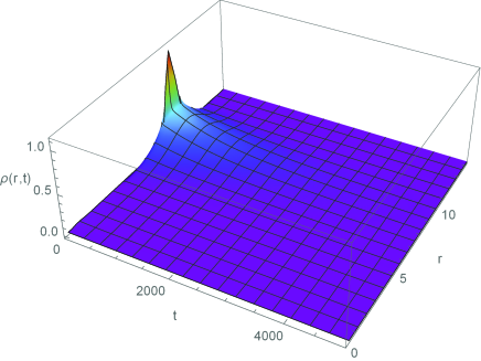
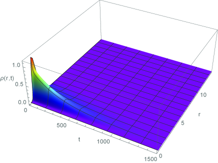
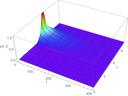
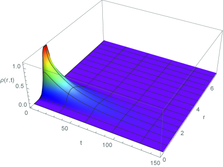
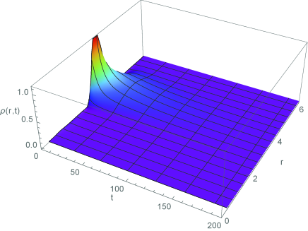
Figure 3: Time evolution of $\rho(r,t)$ in the first passage process of charged dilaton black hole with $b=1,q=1,P=0.003$. (a) $\alpha=0.4$ (b) $\alpha=0.4$ (c) $\alpha=0.2$ (d) $\alpha=0.2$ (e) $\alpha=0$ (f) $\alpha=0$. For the left three graphs, the initial condition is chosen as Gaussian wave pocket located at the large dilaton black hole state while for the right three graphs, the initial condition is chosen as Gaussian wave pocket located at the small dilaton black hole state.

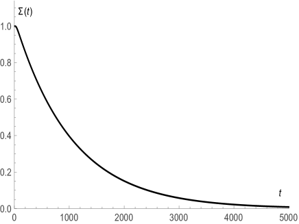
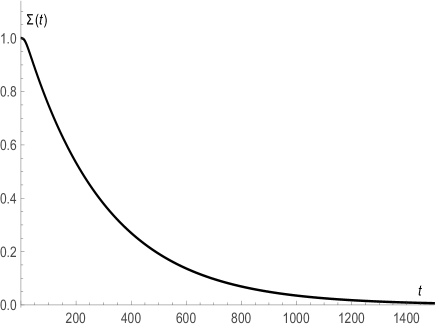
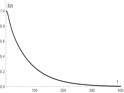
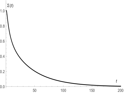
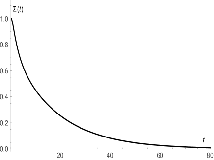
Figure 4: Time evolution of $\Sigma(t)$ for charged dilaton black hole with $b=1,q=1,P=0.003$. (a) $\alpha=0.4$ (b) $\alpha=0.4$ (c) $\alpha=0.2$ (d) $\alpha=0.2$ (e) $\alpha=0$ (f) $\alpha=0$. For the left three graphs, the initial condition is chosen as Gaussian wave pocket located at the large dilaton black hole state while for the right three graphs, the initial condition is chosen as Gaussian wave pocket located at the small dilaton black hole state.

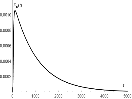
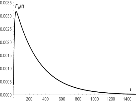
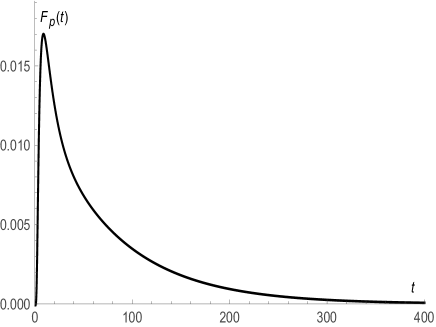
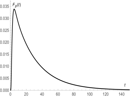
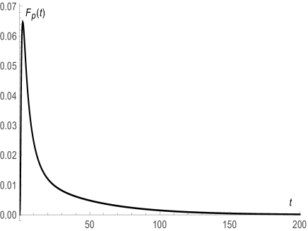
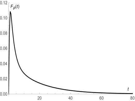
Figure 5: $F_{p}(t)$ for charged dilaton black hole with $b=1,q=1,P=0.003$. (a) $\alpha=0.4$ (b) $\alpha=0.4$ (c) $\alpha=0.2$ (d) $\alpha=0.2$ (e) $\alpha=0$ (f) $\alpha=0$. For the left three graphs, the initial condition is chosen as Gaussian wave pocket located at the large dilaton black hole state while for the right three graphs, the initial condition is chosen as Gaussian wave pocket located at the small dilaton black hole state.

V Conclusions

We probe the effect of dilaon gravity on the dynamic phase transition of black holes by investigating the case of charged dilaton black holes. Specifically, we consider the the variation of the parameter $\alpha$ describing the strength of coupling between the electromagnetic field and the dilaton field.

We introduce the Gibbs free energy landscape and calculate the corresponding $G_{L}$ of the dilaton black hole. Based on $G_{L}$, we can numerically solve the Fokker-Planck equation. To probe the probabilistic evolution of dilaton black holes, we first consider the reflecting boundary condition. When the initial condition is chosen as the large dilaton black hole, the initial peak of $\rho(r,t)$ corresponding to the radius of the large dilaton black hole is decreasing with time while another peak corresponding to the radius of the small dilaton black hole is booming with time. Finally, these two peaks reach a stationary distribution where $\rho(r_{l},t)$ and $\rho(r_{s},t)$ attain the same value. This process clearly illustrates how the initial large dilaton black hole evolves dynamically into the small dilaton black hole. Similar analysis hold for the case that the initial condition is chosen as the small dilaton black hole. The effect of dilaton gravity on the probabilistic evolution of dilaton black holes is quite obvious. Firstly, the horizon radius difference between the large dilaton black hole and small dilaton black hole increases with the parameter $\alpha$. Secondly, with the increasing of $\alpha$, the system needs much more time to achieve a stationary distribution. Note that these two observations do not depend on the initial condition. Thirdly, the value which $\rho(r_{l},t)$ and $\rho(r_{s},t)$ attain varies with the parameter $\alpha$ ($0.229$ for the case of $\alpha=0.4$, $0.250$ for the case of $\alpha=0.2$ and $0.297$ for the case of $\alpha=0$).

To further probe the dynamic phase transition of dilaton black holes, we consider first passage process which describes how the initial black hole state approach the intermediate transition state for the first time. Besides the reflecting boundary condition, absorbing boundary condition should also be imposed here. Resolving the Fokker-Planck equation constrained by these two types of boundary conditions, we show the first passage process of charged dilaon black holes intuitively. No matter what the initial black hole state is, the initial peak decreases very quickly. We compare the evolution for different choices of $\alpha$. The initial peak decays more slowly with the increase of $\alpha$. We also study the distribution of the first passage time $F_{p}(t)$ and the sum of the probability $\Sigma(t)$ that the black hole system having not finished a first passage by time $t$. Irrespective of the initial state, $\Sigma(t)$ decays very fast. The effect of dilaton gravity can also be obviously witnessed. With the increasing of $\alpha$, the decay of $\Sigma(t)$ slows down. There exists one single peak in all the graphs of $F_{p}(t)$, suggesting that the first passage process takes place very fast. And the time corresponding to the peak is found to increase with the parameter $\alpha$.

To conclude, the dilaton field slows down the dynamic phase transition process between the large black hole and the small black hole. It would also be interesting to probe the effect of dilaton field on the dynamic process of novel phase transition disclosed in Ref. Sheykhi16 .

References

- (1) G. W. Gibbons and K. Maeda, Black Holes and Membranes in Higher Dimensional Theories with Dilaton Fields, Nucl. Phys. B 298(1988)741
- (2) D. Garfinkle, G. T. Horowitz and A. Strominger, Charged black holes in string theory, Phys. Rev. D 43(1991)3140
- (3) T. Koikawa and M. Yoshimura, Dilaton Fields and Event Horizon, Phys. Lett. B 189(1987)29
- (4) J. H. Horne and G. T. Horowitz, Rotating dilaton black holes, Phys. Rev. D 46 (1992) 1340-1346
- (5) R. Gregory and J. A. Harvey, Black holes with a massive dilaton, Phys. Rev. D 47(1993)2411
- (6) M. Rakhmanov, Dilaton black holes with electric charge, Phys. Rev. D 50(1994)5155
- (7) S. J. Poletti and D. L. Wiltshire, The Global properties of static spherically symmetric charged dilaton space-times with a Liouville potential, Phys. Rev. D 50(1994)7260
- (8) K. C. K. Chan, J. H. Horne and R. B. Mann, Charged dilaton black holes with unusual asymptotics, Nucl. Phys. B 447(1995)441-464
- (9) P. Kanti, N. E. Mavromatos, J. Rizos, K. Tamvakis and E. Winstanley, Dilatonic black holes in higher curvature string gravity, Phys. Rev. D 54 (1996) 5049-5058
- (10) R. G. Cai, J. Y. Ji and K. S. Soh, Topological dilaton black holes, Phys. Rev D 57(1998)6547
- (11) D. Grumiller, W. Kummer and D. V. Vassilevich, Dilaton gravity in two-dimensions. Phys. Rept. 369 (2002) 327-430
- (12) G. Clement, D. Gal’tsov and C. Leygnac, Linear dilaton black holes, Phys. Rev. D 67(2003)024012
- (13) G. Clement and C. Leygnac, Non-asymptotically flat, non-AdS dilaton black holes, Phys. Rev. D 70(2004)084018
- (14) C. J. Gao and H. N. Zhang, Higher dimensional dilaton black holes with cosmological constant, Phys. Lett. B 605 (2005) 185-189
- (15) C. J. Gao and H. N. Zhang, Dilaton black holes in de Sitter or Anti-de Sitter universe, Phys. Rev. D 70 (2004) 124019.
- (16) C. J. Gao and H. N. Zhang, Topological Black Holes in Dilaton Gravity Theory, Phys. Lett. B 612(2006)127-136
- (17) A. Sheykhi, N. Riazi and M. H. Mahzoon, Asymptotically non-flat Einstein-Born-Infeld-dilaton black holes with Liouville-type potential, Phys. Rev. D 74 (2006) 044025
- (18) A. Sheykhi, N. Riazi, Thermodynamics of black holes in -dimensional Einstein-Born-Infeld dilaton gravity, Phys. Rev. D75(2007)024021
- (19) A. Sheykhi, M. H. Dehghani, S. H. Hendi, Thermodynamic Instability of Charged Dilaton Black Holes in AdS Spaces, Phys. Rev. D 81(2010)084040
- (20) A. Sheykhi and S. Hajkhalili, Dilaton black holes coupled to nonlinear electrodynamic field, Phys. Rev. D 89(2014)104019
- (21) A. Sheykhi and A. Kazemi, Higher dimensional dilaton black holes in the presence of exponential nonlinear electrodynamics, Phys. Rev. D 90(2014)044028
- (22) M. K. Zangeneh, A. Sheykhi and M. H. Dehghani, Thermodynamics of higher dimensional topological dilation black holes with a power-law Maxwell field, Phys. Rev. D 91(2015)044035
- (23) A. Sheykhi, F. Naeimipour and S. M. Zebarjad, Phase transition and thermodynamic geometry of topological dilaton black holes in gravitating logarithmic nonlinear electrodynamics, Phys. Rev. D 91(2015)124057
- (24) A. Sheykhi, F. Naeimipour and S. M. Zebarjad, Thermodynamic geometry and thermal stability of -dimensional dilaton black holes in the presence of logarithmic nonlinear electrodynamics, Phys. Rev. D 92(2015)124054
- (25) M. H. Dehghani, A. Sheykhi and Z.Dayyani, Critical behavior of Born-Infeld dilaton black holes, Phys. Rev. D 93(2016)024022
- (26) A. Sheykhi, Thermodynamics of charged topological dilaton black holes, Phys. Rev. D 76 (2007) 124025
- (27) R. Zhao, H. H. Zhao, M. S. Ma and L. C. Zhang, On the critical phenomena and thermodynamics of charged topological dilaton AdS black holes, Eur. Phys. J. C73 (2013) 2645
- (28) M. H. Dehghani, S. Kamrani and A. Sheykhi, - criticality of charged dilatonic black holes, Phys. Rev. D 90(2014)104020
- (29) S. H. Hendi, A. Sheykhi, S. Panahiyan and B. Eslam Panah, Phase transition and thermodynamic geometry of Einstein-Maxwell-dilaton black holes, Phys. Rev. D92 (2015)064028
- (30) A. Dehyadegari, A. Sheykhi and A. Montakhab, Novel phase transition in charged dilaton black holes, Phys. Rev. D 96 (2017) 8, 084012
- (31) J. X. Mo, An alternative perspective to observe the critical phenomena of dilaton black holes, Eur. Phys. J. C 77 (2017) 8, 529
- (32) Y. Chen, H. Li and S. J. Zhang, Microscopic explanation for black hole phase transitions via Ruppeiner geometry: Two competing factors Cthe temperature and repulsive interaction among BH molecules, Nucl. Phys. B 948 (2019) 114752
- (33) Q. Q. Jiang, S. Q. Wu, X. Cai, Hawking radiation from the dilatonic black holes via anomalies, Phys. Rev. D 75 (2007) 064029
- (34) D. Y. Chen, Q. Q. Jiang, S. Z. Yang and X. T. Zu, Fermions tunnelling from the charged dilatonic black holes, Class. Quant. Grav. 25 (2008) 205022
- (35) K. Goldstein, S. Kachru, S. Prakash and S. P. Trivedi, Holography of Charged Dilaton Black Holes, JHEP 1008(2010)078
- (36) K. Goldstein, N. Lizuka, S. Kachru, S. Prakash, S. P. Trivedi and A. Westphal, Holography of Dyonic Dilaton Black Branes, JHEP 1010(2010)027
- (37) C. M. Chen and D. W. Peng, Holography of Charged Dilaton Black Holes in General Dimensions, JHEP 1006(2010)093
- (38) S. S. Gubser, F. D. Rocha, Peculiar Properties of a Charged Dilatonic Black Hole in Ad, Phys. Rev. D81(2010)046001
- (39) B. Gouteraux, B. S. Kim and R. Meyer, Charged Dilatonic Black Holes and Their Transport Properties, Fortschr. Phys. 59(2011)723
- (40) W. J. Li, Some Properties of the Holographic Fermions in an Extremal Charged Dilatonic Black Holes, Phys. Rev. D84(2011)064008
- (41) Y. C. Ong and P. Chen, Stringy Stability of Charged Dilaton Black Holes with Flat Event Horizon, JHEP 1208(2012)79
- (42) W. J. Li, R. Meyer and H. Zhang, Holographic Non-Relativistic Fermionic Fixed Point by the Charged Dilatonic Black Hole, JHEP 01 (2012) 153
- (43) J. X. Mo, G. Q. Li and X. B. Xu, Effects of power-law Maxwell field on the critical phenomena of higher dimensional dilaton black holes, Phys. Rev. D 93 (2016)084041
- (44) S. Soroushfar, R. Saffari, E. Sahami,Geodesic equations in the static and rotating dilaton black holes: Analytical solutions and applications, Phys.Rev.D 94 (2016) 2, 024010
- (45) E. W. Hirschmann, L. Lehner, S. L. Liebling, C. Palenzuela, Black Hole Dynamics in Einstein-Maxwell-Dilaton Theory, Phys.Rev.D 97 (2018) 6, 064032
- (46) A. Li, H. Shi and D. Zeng, Phase structure and quasinormal modes of a charged AdS dilaton black hole, Phys. Rev. D 97 (2018) 2, 026014
- (47) T. Y. Yu, W. Y. Wen, Cosmic censorship and Weak Gravity Conjecture in the Einstein CMaxwell-dilaton theory, Phys. Lett. B 781 (2018) 713-718
- (48) M. Dehghani, Thermodynamic properties of dilaton black holes with nonlinear electrodynamics, Phys. Rev. D 98 (2018) 4, 044008
- (49) J. V. Rocha, M. Tomašević, Self-similarity in Einstein-Maxwell-dilaton theories and critical collapse, Phys.Rev.D 98 (2018) 10, 104063
- (50) M. Dehghani, Thermodynamics of novel dilatonic BTZ black holes coupled to Born-Infeld electrodynamics, Phys. Rev. D 99 (2019) 2, 024001
- (51) M. Dehghani, M. R. Setare, Dilaton black holes with power law electrodynamics, Phys. Rev. D 100 (2019) 4, 044022
- (52) P. Aniceto, J. V. Rocha, Self-similar solutions and critical behavior in Einstein-Maxwell-dilaton theory sourced by charged null fluids, JHEP 10 (2019) 151
- (53) D. Astefanesei, J. L. Bl zquez-Salcedo, C. Herdeiro, E. Radu, N. Sanchis-Gual, Dynamically and thermodynamically stable black holes in Einstein-Maxwell-dilaton gravity, Phys. Rev. D 101 (2020) 12, 124017
- (54) M. M. Stetsko, Static spherically symmetric Einstein-Yang-Mills-dilaton black hole and its thermodynamics, Phys. Rev. D 101 (2020) 12, 124017
- (55) S. Yu, J. Qiu and C. Gao, Constructing black holes in Einstein-Maxwell-scalar theory, Class. Quant. Grav. 38 (2021) 10, 105006
- (56) C. Y. Zhang, P. Liu, Y. Liu, C. Niu and B. Wang, Evolution of Anti-de Sitter black holes in Einstein-Maxwell-dilaton theory, arXiv: 2104.07281
- (57) R. Li and J. Wang, Thermodynamics and kinetics of Hawking-Page phase transition, Phys. Rev. D 102 (2020) 2, 024085.
- (58) R. Li, K. Zhang and J. Wang, Thermal dynamic phase transition of Reissner-Nordström Anti-de Sitter black holes on free energy landscape, JHEP 10 (2020) 090.
- (59) R. Li and J. Wang, Energy and entropy compensation, phase transition and kinetics of four dimensional charged Gauss-Bonnet Anti-de Sitter black holes on the underlying free energy landscape, arXiv: 2012.05424.
- (60) S. W. Wei, Y. Q. Wang, Y. X. Liu and R. B. Mann, Dynamic properties of thermodynamic phase transition for five-dimensional neutral Gauss-Bonnet AdS black hole on free energy landscape, arXiv: 2009.05215.
- (61) S. W. Wei, Y. Q. Wang, Y. X. Liu and R. B. Mann, Observing dynamic oscillatory behavior of triple points among black hole thermodynamic phase transitions, arXiv: 2102.00799.
- (62) Shan-Quan Lan, Jie-Xiong Mo, Gu-Qiang Li and Xiao-Bao Xu, Effects of dark energy on dynamic phase transition of charged AdS black holes, arXiv: 2104.11553.
- (63) R. Li, K. Zhang and J. Wang, Probing black hole microstructure with the kinetic turnover of phase transition, arXiv: 2102.09439.
- (64) R. Zwanzig, Nonequilibrium Statistical Mechanics, Oxford University Press (2001).
- (65) C.-L. Lee, C.-T. Lin, G. Stell and J. Wang, Diffusion dynamics, moments, and distribution of first-passage time on the protein-folding energy landscape, with applications to single molecules, Phys. Rev. E 67 (2003) 041905.
- (66) C.-L. Lee, G. Stell and J. Wang, First-passage time distribution and non-Markovian diffusion dynamics of protein folding, J.Chem.Phys. 118 (2003) 959.
- (67) J. Wang, Landscape and flux theory of non-equilibrium dynamical systems with application to biology, Adv.Phys. 64 (2015) 1.
- (68) J. D. Bryngelson and P. G. Wolynes, Intermediates and Barrier Crossing in a Random Energy Model (with Applications to Protein Folding), J.Phys.Chem. 93 (1989) 6902.