On the Pareto Front of Physics-Informed Neural Networks

Abstract

Recently a new type of deep learning method has emerged, called physics-informed neural networks. Despite their success in solving problems that are governed by partial differential equations, physics-informed neural networks are often difficult to train. Frequently reported convergence issues are still poorly understood and complicate the inference of correct system dynamics. In this paper, we shed light on the training process of physics-informed neural networks. By trading between data- and physics-based constraints in the network training, we study the Pareto front in multi-objective optimization problems. We use the diffusion equation and Navier-Stokes equations in various test environments to analyze the effects of system parameters on the shape of the Pareto front. Additionally, we assess the effectiveness of state-of-the-art adaptive activation functions and adaptive loss weighting methods. Our results demonstrate the prominent role of system parameters in the multi-objective optimization and contribute to understanding convergence properties of physics-informed neural networks.

Keywords physics-informed neural networks  $\cdot$ Pareto front  $\cdot$ multi-objective optimization  $\cdot$ system parameters

1 Introduction

Artificial Neural Networks (ANNs) are well known for their capability to approximate any continuous function $f:\mathbb{R}^{d}\to\mathbb{R}^{D}$ when given appropriate weights [1, 2]. The flexibility and expressive power of ANNs and variants has led to tremendous success in a wide range of applications, including image recognition [3], natural language processing [4] or generative modeling [5]. Recently, a new kind of use case for ANNs has emerged, called physics-informed deep learning. Various methods, among them physics-informed neural networks (PINNs), have been successfully used in solving physical related problems where classical approaches are limited [6, 7, 8]. Today, PINNs are widespread in diverse scientific and engineering disciplines, such as bio-engineering [9, 10], aerodynamics [11, 12] or materials science [13, 14].

The general idea of physics-informed deep learning is to reduce the space of admissible solutions to those that fulfill certain physical laws, e.g. conservation of energy, momentum or mass. The governing equations usually come in form of partial differential equations (PDEs) and act as additional constraints during the network training. A standard approach in PINNs is to encode the physical constraints through a suitable loss function [15, 16]. The resulting physics-based loss competes against a data-based loss which is needed to provide essential information on the system under study. The multi-objective optimization of data and physics gives PINNs large-scale flexibility in solving forward and inverse problems involving PDEs. Along with the application as a surrogate model for solving PDEs [7, 11, 17], PINNs can make further use of additional data from measurements or simulations to augment data-driven solutions when the correct form of the PDE is known [18, 19]. On the other hand, missing knowledge on the underlying physical system, e.g. on coefficients of the governing equations, can be inferred through data-driven discovery of governing PDEs [16, 13, 12, 20].

Setting up a well-working PINN application, however, can be precarious and laborious. Besides design choices, e.g. finding a suitable network architecture or activation function, frequently occurring convergence issues in the multi-objective optimization complicate a straight-forward use of PINNs [7, 21, 22, 23]. As a concrete example, Figure 1 demonstrates the failure of a PINN when solving the one-dimensional diffusion equation. Here, data- and physics-based loss are equally weighted in the network training which apparently led to a large discrepancy between true and predicted system dynamics. The importance of using a hyper-parameter that trades between individual losses is well-known from multi-objective optimization [24, 25] and has been discussed several times in the context of PINNs [21, 26]. Individual losses are often weighted manually on a try-and-see basis in order to determine optimal settings for a specific task [26]. Recently, self-adaptive methods have been proposed to improve the accuracy and facilitate the multi-objective optimization of PINNs [21, 26]. An alternative strategy is studied in references [27, 28] where adaptive activation functions are used to improve the convergence and accuracy of PINNs. The adaptive activation functions change dynamically the topology of the loss function which strives for an improved convergence rate in the model training. Further studies, e.g. on the spectral bias [23] among others [29, 30], gave a theoretical perspective on the training process and uncertainty quantification of PINNs. Still, the accuracy and effectiveness of PINNs can barely be predicted in advance and proposed solutions to the convergence problem are often optimized for a specific application.

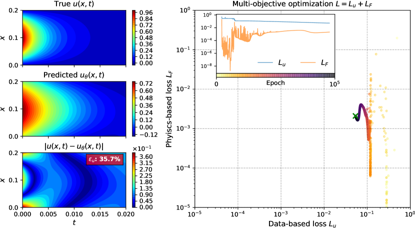
Figure 1: PINN failure. Left: large discrepancy between true and predicted solution function for the diffusion equation, see problem setup 3.1. Relative $\ell^{2}$-error is measured on a test set and given in the red box. Right: intermediate gradient descent steps of the multi-objective optimization using the unweighted linear combination of data-based loss $L_{u}$ and physics-based loss $L_{F}$. The green cross indicates the final position to which gradient-descent optimization has converged. Inset: learning curves as function of training epochs. Further details on the used network and data settings can be found in section 4 and 4.1.

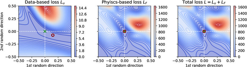
Figure 2: Pareto optimum. Loss landscapes at final position of gradient descent optimization, see green cross in Figure 1. Red circles indicate minimum loss in the vicinity of the current position (green crosses). At this Pareto optimum, the data-based loss (left) cannot be further decreased without increasing the physics-based loss (middle). The total loss (right) is given as the unweighted linear combination of both losses. Loss landscapes were constructed using visualization techniques from reference [31].

In this work, we provide insight into the training process of PINNs by qualitatively analysing the Pareto front of the multi-objective optimization. In general, the Pareto front in multi-objective optimization is the set of Pareto-optimal solutions that are feasible by the optimization algorithm. A Pareto optimum is a state where an individual loss cannot be further decreased without increasing at least one of the others. As an example, Figure 2 visualizes the Pareto optimum attained in the unweighted multi-objective optimization of Figure 1. Here, the data-based loss cannot be minimized further without increasing the physics-based loss. As a consequence, further training stops at a solution that lacks of information coming from the data. Since in this example the data provides essential information on initial and boundary conditions, a large discrepancy between true and predicted solutions can be observed, see left panel of Figure 1. Applying an additional loss weight on either data- or physics-based loss, or both, may direct the multi-objective to a different Pareto optimum. Whether at the new attained optimum the inferred solution is in a better agreement with the true solution cannot be predicted in advance and is determined by the innate shape of the Pareto front.

The Pareto front is influenced by many factors including model-specific design choices as the network architecture, loss terms or activation function. In connection with PINNs, also system parameters such as the system scale or parametrization coefficients of governing PDEs have an influence on the shape of the Pareto front. These system parameters are manifold in certain applications and contribute to the complexity of the problem. One way to reduce the set of system parameters is non-dimensionalization or system scaling. This concept gives us a controllable setting in which we can study the influence of system parameters on various test environments using the (i) diffusion equation and (ii) Navier-Stokes equations.

The paper is structured as follows. In section 2, we first introduce the methodology in use, including the fundamental working method of PINNs and multi-objective optimization of data- and physics-based loss. Next, in section 3 the problem setup for scaled systems using the (i) diffusion equation and (ii) Navier-Stokes equations is discussed. In section 4 we present our results and provide further discussion in section 5. Additional in section 4 and 5, we analyse the effectiveness of a state-of-the-art adaptive activation function and adaptive loss weighting. Finally, section 6 summarizes our findings and provide a closing discussion on future directions.

2 Methodology

2.1 Physics-Informed Neural Networks

To briefly demonstrate the fundamental working method of PINNs we consider a two-dimensional physical system which is described by a single PDE - the extension to higher dimensional systems involving one or multiple PDEs is straightforward and will be discussed later on. For a complete description of PINNs, the reader is referred to reference [16]. For the two-dimensional case, the implicit form of a PDE with solution function $u$ is given by

$$F\left(x_{1},x_{2},u(x_{1},x_{2}),\frac{\partial u(x_{1},x_{2})}{\partial x_{1}},...,\frac{\partial^{2}u(x_{1},x_{2})}{\partial x_{1}\partial x_{2}},...,\frac{\partial^{k}u(x_{1},x_{2})}{\partial x_{2}^{k}};\lambda\right)=0,$$ (1)

where $F(\cdot\,;\lambda)$ represents an arbitrary function with partial derivatives up to order $k$ and parametrization $\lambda$. Here, and in the further course of this paper, we only consider well-posed problems, i.e. problems with a unique solution function $u$ that fulfills equation (1) in the domain $(x_{1},x_{2})\in\Omega$. Well-posed problems are usually specified with sufficient initial/boundary conditions on $(x_{1},x_{2})\in\partial\Omega$, such that there is no ambiguity in the solution function on the domain $\Omega$. In this work, the PDE’s parametrization $\lambda$ and the computational domain $\Omega$ are considered as system-specific parameters and, thus, referred to as system parameters.

We further proceed by approximating the solution function $u(x)$ by an ANN $u_{\theta}(x)$ with parameters $\theta$. As a common approach in supervised machine learning, the neural network function can be updated with labeled data $\{x^{(i)},u^{(i)}\}_{i=1}^{N_{u}}$ and a suitable data-based loss function. Data can be used to encode initial/boundary conditions or to incorporate measured or simulated data from inside the function domain. To train the ANN with the available data, we choose following data-based loss function

$$L_{u}(\theta)=\frac{1}{N_{u}}\sum_{i=1}^{N_{u}}\left|u_{\theta}(x^{(i)})-u^{(i)}\right|^{2}.$$ (2)

To encode the physical constraints in the neural network training, we make use of automatic differentiation [32] as found in open source software libraries as e.g. Tensorflow [33] or PyTorch [34]. With automatic differentiation, derivatives of the neural network function $\partial u_{\theta}/\partial x$ can be evaluated at specified coordinates, commonly described as collocation points. Derivatives can be evaluated up to the order the neural network activation function is differentiable. Commonly used activation function in PINNs are the hyperbolic tangent (tanh), sinusoidal (sin) or swish, each is continuously differentiable. With the neural network derivatives as "building block", residuals of equation (1) can be evaluated at the collocation points - here it should be apparent that this approach can be followed for any kind of PDE. The ANN is constrained to satisfy equation (1) at the specified collocation points $\{x_{\mathrm{col}}^{(i)}\}_{i=1}^{N_{\mathrm{col}}}$ by minimizing following physics-based loss:

$$L_{F}(\theta)=\frac{1}{N_{\mathrm{col}}}\sum_{i=1}^{N_{\mathrm{col}}}\left|F\left(x_{\mathrm{col}}^{(i)},u_{\theta}(x_{\mathrm{col}}^{(i)}),\frac{\partial u_{\theta}(x_{\mathrm{col}}^{(i)})}{\partial x};\lambda\right)\right|^{2}.$$ (3)

Here, $F$ denotes the evaluated residuals of equation (1) using the neural network function and its derivatives. As there is no restriction in the choice of collocation points, they can be randomly sampled from inside the function domain, e.g. using hyper-cube sampling. This gives PINNs a great advantages over classical PDE solvers, e.g. finite difference, finite volume or finite element method, that rely on a cumbersome construction of a computational mesh. Common approaches in PINNs are a fixed set of collocation points, a newly sampled set at each iteration or adaptively chosen points based on the residuals of the PDE [35, 36, 37].

2.2 The Pareto Front in Multi-objective Optimization

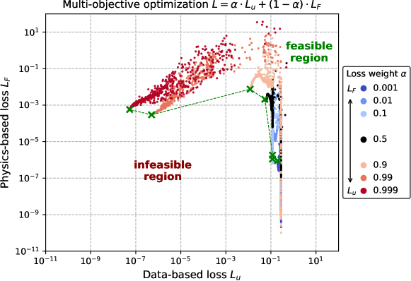
Figure 3: Pareto Front. A representative sample of the loss weight $\alpha$ is used to qualitatively scan the Pareto front of the multi-objective optimization of data-based loss $L_{u}$ and physics-based loss $L_{F}$. The approximated Pareto front (green dashed line) can be seen as the theoretical interpolation of all possible Pareto optima (green crosses). Solutions beyond the Pareto front are in general infeasible. Results were obtained using the problem definition from Figure 1 with the multi-objective optimization (5).

Since PINNs try to minimize a data- and a physics-based loss function, their training is a multi-objective optimization problem. Vanilla PINNs follow the standard approach in multi-objective optimization and use a linear, unweighted combination of the individual losses

$$L(\theta)=L_{u}(\theta)+L_{F}(\theta).$$ (4)

Given the definition of the data-based loss (2) and physics-based loss (3), and the expressive power of ANNs, it would be legitimate to expect no contradiction in the loss definition (4) – a perfectly learned solution function yields zero loss on both. Still, it has been frequently reported and shown in Figure 1 that for PINNs the simple linear combination of data- and physics-based loss potentially leads to a model failure as the minimization of one of the two losses stalls during model training. Consequently, we introduce a hyper-parameter that trades between the two losses in the multi-objective optimization as following

$$L(\theta;\alpha)=\alpha\cdot L_{u}(\theta)+(1-\alpha)\cdot L_{F}(\theta)\quad\quad\alpha\in(0,1).$$ (5)

According to this definition, for $\alpha\to 1$, greater loss weight is put on the data-based loss, while for $\alpha\to 0$ on the physics-based loss. A loss weight of $\alpha=0.5$ relates to an unweighted multi-objective optimization.

In general, the Pareto front of a multi-objective optimization is hard to visualize. With our multi-objective loss definition (5), the Pareto front can be seen as the theoretical interpolation of all possible Pareto optima that are attained by a continuous adjustment of the loss weight $\alpha$. Solutions beyond the Pareto front, in general, are infeasible. For the scope of this work, we take a representative sample in the range of $\alpha\in(0,1)$ to qualitatively scan the Pareto front. As an example, Figure 3 shows the Pareto optima for a few selected values of the loss weight $\alpha$. For clarity, the Pareto front, as well as the feasible and infeasible regions, are explicitly visualized in the figure.

In multi-objective optimization, the general goal is to obtain a Pareto optimum where all individual losses are low. Every so often, however, those solutions are infeasible due to the innate shape of the Pareto front. When the Pareto front is convex, the mapping between loss weights $\alpha$ and the corresponding point on the Pareto front is well-behaved, as small changes in $\alpha$ lead to small changes in the convergence points. This behaviour allows to select adequate solutions by sweeping $\alpha$. For concave parts of the Pareto front, sweeping the loss weight is delicate, as small changes in $\alpha$ may lead to the optimization converging to few dominating areas on the Pareto front (e.g. for 0.99 and 0.999, or 0.001, 0.01 and 0.1 in Figure 3, respectively). Usually, the optimal choice is determined on a try-and-see-basis by comparing the PINN’s solution to the true solution. This approach may be elusive if the true solution of the underlying problem is a priori unknown.

Whether the Pareto front is convex, concave or a mixture of both, is determined by several factors. Common design choices, e.g. the network architecture or activation function, may influence the shape of the Pareto front. The definition of individual objectives, here given by the data- and physics-based loss, is another cause that influences the shape of the Pareto front. So far, little focus was put on the influence of system parameters as the system scale or parametrization coefficient of governing PDEs.

3 Problem Setup

In the following section we discuss the problem setup and test environments using the (i) diffusion equation and (ii) Navier-Stokes equations. We give a proper definition of the governing PDEs, initial and boundary conditions, as well as a derived analytical solution for scaled systems. In both examples we introduce a characteristic system dimension $M$ which is used to adjust the scale of the system.

3.1 Diffusion Equation

The diffusion equation, along with variants thereof, is among the most widely studied parabolic PDEs with applications in many fields of science, pure mathematics and engineering. In this work, we study the heat equation, a special case of the diffusion equation in the context of engineering. Specifically, we consider the cooling of a one-dimensional rod with an initial temperature distribution and Dirichlet boundary conditions on both rod ends. The dynamics of the system are described by the equation

$$F\equiv\frac{\partial u(x,t)}{\partial t}-\kappa\frac{\partial^{2}u(x,t)}{\partial x^{2}}=0.$$ (6)

Here, the solution function $u$ denotes the temperature of the rod at position $x$ and time $t$, and $\kappa$ is the parametrization coefficient, commonly known as thermal diffusivity. We define the initial (IC) and boundary (BC) conditions as following

$$\mathrm{IC} : u(x,0)=\text{sin}\left(\pi\frac{x}{M}\right) 0\leq x\leq M,$$ (7)

$$\mathrm{BC} : u(0,t)=u(M,t)=0 t<0,$$ (8)

with $M$ denoting the length of the rod which, in this context, is the characteristic length scale of the system. The problem stated above is well-posed and has a unique solution

$$u(x,t)=\text{sin}\left(\pi\frac{x}{M}\right)\cdot e^{-\frac{\kappa\pi^{2}}{M^{2}}t}.$$ (9)

In this example, training data for the initial (7) and boundary (8) conditions are feed to the PINN through a composite data-based loss function

$$L_{u}(\theta) =L_{\mathrm{IC}}(\theta)+L_{\mathrm{BC}}(\theta),$$ (10a)

$$L_{\mathrm{IC}}(\theta) =\frac{1}{N_{\mathrm{IC}}}\sum_{i=1}^{N_{\mathrm{IC}}}\left|u_{\theta}(x_{\mathrm{IC}}^{(i)},t_{\mathrm{IC}}^{(i)})-u_{\mathrm{IC}}^{(i)}\right|^{2},$$ (10b)

$$L_{\mathrm{BC}}(\theta) =\frac{1}{N_{\mathrm{BC}}}\sum_{i=1}^{N_{\mathrm{BC}}}\left|u_{\theta}(x_{\mathrm{BC}}^{(i)},t_{\mathrm{BC}}^{(i)})-u_{\mathrm{BC}}^{(i)}\right|^{2},$$ (10c)

where $\{(x_{\mathrm{IC}}^{(i)},t_{\mathrm{IC}}^{(i)}),u_{\mathrm{IC}}^{(i)}\}_{i=1}^{N_{\mathrm{IC}}}$ and $\{(x_{\mathrm{BC}}^{(i)},t_{\mathrm{BC}}^{(i)}),u_{\mathrm{BC}}^{(i)}\}_{i=1}^{N_{\mathrm{BC}}}$ are the datasets for the IC and BC, respectively. The physics-based loss is constructed using the PDE (6) in the loss definition (3) and a suitable set of collocation points $\{(x_{\mathrm{col}}^{(i)},t_{\mathrm{col}}^{(i)})\}_{i=1}^{N_{\mathrm{col}}}$. Furthermore, data- and physics-based loss are minimized through the multi-objective loss (5).

3.2 Navier-Stokes Equations

The Navier-Stokes equations are the governing PDEs in the study of fluid flow. Along with the continuity equation, they describe the conservation of momentum and mass of viscous fluids. Their importance in scientific and engineering modeling is indisputable as they are applied to many physical phenomena occurring in weather forecast, blood flow through vessels or flow around obstacles. For our study, we limit the application to a two-dimensional, incompressible steady-state flow where the mapping to be learned by the PINN is given by the vector-valued function $(x,y)\mapsto(u,v,p)$. The governing equations for the conservation of momentum in $\mathrm{x}$- and $\mathrm{y}$-direction and mass are given in respective order by

$$F_{\mathrm{x}} \equiv\left(u\frac{\partial u}{\partial x}+v\frac{\partial u}{\partial y}\right)+\frac{1}{\rho}\frac{\partial p}{\partial x}-\nu\left(\frac{\partial^{2}u}{\partial x^{2}}+\frac{\partial^{2}u}{\partial y^{2}}\right)=0,$$ (11a)

$$F_{\mathrm{y}} \equiv\left(u\frac{\partial v}{\partial x}+v\frac{\partial v}{\partial y}\right)+\frac{1}{\rho}\frac{\partial p}{\partial y}-\nu\left(\frac{\partial^{2}v}{\partial x^{2}}+\frac{\partial^{2}v}{\partial y^{2}}\right)=0,$$ (11b)

$$F_{\mathrm{c}} \equiv\frac{\partial u}{\partial x}+\frac{\partial v}{\partial y}=0,$$ (11c)

where $u$, $v$ and $p$ denote the fluid velocity in $\mathrm{x}$- and $\mathrm{y}$-direction and pressure in respective order, and $\rho$ and $\nu$ are fluid-specific quantities, denoting the density and viscosity of the fluid. Analytical solutions in fluid dynamics are scarce. Therefore, we consider the laminar fluid flow in the wake of a two-dimensional grid which has been solved analytically [38]. With $M$ as the characteristic spacing of the grid, $u_{0}$ the mean velocity in $\mathrm{x}$-direction and assuming $\rho=1$, the analytical solution for the flow velocities $u$ and $v$, and pressure $p$ is described by

$$u(x,y) =u_{0}\cdot\left(1-e^{\gamma\frac{x}{M}}\cdot\text{cos}\left(2\pi\frac{y}{M}\right)\right),$$ (12a)

$$v(x,y) =\frac{u_{0}\gamma}{2\pi}\cdot e^{\gamma\frac{x}{M}}\cdot\text{sin}\left(2\pi\frac{y}{M}\right),$$ (12b)

$$p(x,y) =u_{0}^{2}\cdot e^{2\gamma\frac{x}{M}}+C,$$ (12c)

where $C$ is a constant and $\gamma$ is expressed by

$$\gamma=\frac{1}{2\nu}-\sqrt{\frac{1}{4\nu^{2}}+4\pi^{2}}.$$ (13)

The solution stated above can be derived by assuming a fixed relation between the grid spacing and reference velocity of the flow, here $M\cdot u_{0}=1$ [38]. Under these assumptions, the Reynolds number of the fluid flow is given by $Re=1/\nu$ and, thus, any selected grid spacing $M$ catches the intrinsic properties of the fluid flow at the given viscosity or Reynolds number.

For this example, the PINN is trained on boundary data which is sampled from the analytical solution of the flow velocities (12a) and (12b) at the boundary. Since the flow is steady state, there are no initial conditions. The pressure is entirely learned by the PINN and inferred through the set of governing PDEs. The set of PDEs (11) are combined in a composite physics-based loss through

$$L_{F}(\theta)=L_{F,\mathrm{x}}(\theta)+L_{F,\mathrm{y}}(\theta)+L_{F,\mathrm{c}}(\theta),$$ (14)

where $L_{F,\mathrm{x}}$, $L_{F,\mathrm{y}}$ and $L_{F,\mathrm{c}}$ are constructed using the individual PDEs (11) in the loss definition (3). Again, data- and physics-based loss are minimized using the multi-objective loss (5).

4 Results

In this section, we apply the introduced methodology to solve (i) the diffusion equation and (ii) Navier-Stokes equations, as given in the problem setup section 3. Additionally in subsection 4.3, we perform tests on solving the diffusion equation by using a state-of-the-art adaptive activation function and adaptive loss weighting method in the multi-objective optimization.

All following tests are conducted using a standard 4x50 network architecture with hyperbolic tangent activation function and Adam optimizer [39] with full-batch training and exponential learning rate decay. The output neurons use a linear activation function and all layer weights are initialized using the Glorot uniform initializer [40]. A preliminary grid search for optimal hyper-parameters has shown that under these design choices and for a decay step size of 1000, the ideal initial learning rate and rate decay is 0.01 and 0.9, respectively. Default settings for the momentum in Adam are used and the maximum number of epochs is set to 100k. Different test runs are conducted using new seeds for data sampling and parameter initialization. For clarity in the visualizations, a single test run is picked. In both problem setups (i) and (ii), we select three system scales by using $M=[0.2,1,5]$. Model training is performed on a Nvidia Tesla P100-PCIe-16GB graphics card and all code is implemented in TensorFlow 2.1 [33].

To evaluate the model’s accuracy, we measure the prediction error against the analytical solution on an independent test set in term of the relative $\ell^{2}$-error

$$\epsilon_{u}\equiv\frac{\|u-u_{\theta}\|_{2}}{\|u\|_{2}}.$$ (15)

4.1 Diffusion Equation

In order to provide comparable test environments for different scaled systems, we introduce the characteristic diffusive time scale $T=M^{2}/\kappa$. Subsequently, we consider a computational domain $(x,t)\in\Omega\equiv[0,M]\otimes[0,T/2]$ in which the solution function (9) captures the intrinsic diffusion process. In the following tests, the training data for IC, BC, collocation and the test set are randomly sampled with sizes $N_{\mathrm{IC}}=100$, $N_{\mathrm{BC}}=200$, $N_{\mathrm{col}}=2500$ and $N_{\mathrm{test}}=1000$, respectively.

As a first test, we choose a thermal diffusivity $\kappa=1$ and consider the unweighted multi-objective optimization by taking $\alpha=0.5$ in the loss definition (5). The results for the system scales $M=[0.2,1,5]$ are shown column wise in Figure 4. The first row shows the analytical solution for each respective system scale, the second row the learned function after the full model training, and the third row depicts the residual error distribution on the entire function domain. The measured relative $\ell^{2}$-errors on the test set are given as red boxes in the residual error plots. Although the system dynamics to be learned is similar for each system scale and equal model settings were used, strong variations in the accuracy of the learned function can be observed. For $M=1$ (middle panel) and $M=5$ (right panel) the model’s prediction is in good agreement with the analytical solution ($\epsilon_{u}<0.015\%$). The model performing on $M=0.2$ (left panel), however, fails to accurately catch the correct system dynamics ($\epsilon_{u}\approx 36\%$), which has been already demonstrated in Figure 1.

To further analyse this behaviour and the multi-objective optimization, we keep the system settings from the previous test, but trade between the data- and physics-based loss by adjusting the loss weight $\alpha$. Figure 5 illustrates the training and test performance measures as intermediate steps of the gradient descent optimization. The first row shows the data-based loss $L_{u}$ plotted against the physics-based loss $L_{F}$, as already used in Figure 3. In addition, the measured relative $\ell^{2}$-errors on the test set as a function of training iterations are shown in the second row of Figure 5. Here we note, that special caution was put on a sufficiently long training duration and further training would not significantly reduce the measured quantities. That is to say, gradient descent has converged to the Pareto optima. While for the system scale $M=5$ (right panel) the Pareto optima clearly lie on a convex-shaped Pareto front, the Pareto front of the system scale $M=0.2$ (left panel) forms a concave shape. The Pareto front for system scale $M=1$ (middle panel) has both convex and concave parts. From these results it is evident that the unweighted multi-objective optimization ($\alpha=0.5$), as shown in Figure 4, converges to distant Pareto optima that are determined by the innate shape of the Pareto front for the specific system scale. When looking on the measured relative $\ell^{2}$-errors in Figure 5, it is also apparent that for $M=5$ any choice for the loss weight, except for $\alpha\to 1$, would lead to a good model performance due to the Pareto front being convex. For $M=0.2$, on the other hand, only loss weights with $\alpha\to 1$ would lead to accurate results since the concave-shaped Pareto front renders other solutions impractical. Again, the system scale $M=1$ can be seen as intermediate trend of both where, in general, greater loss weights on the data-based loss ($\alpha\to 1$) perform better.

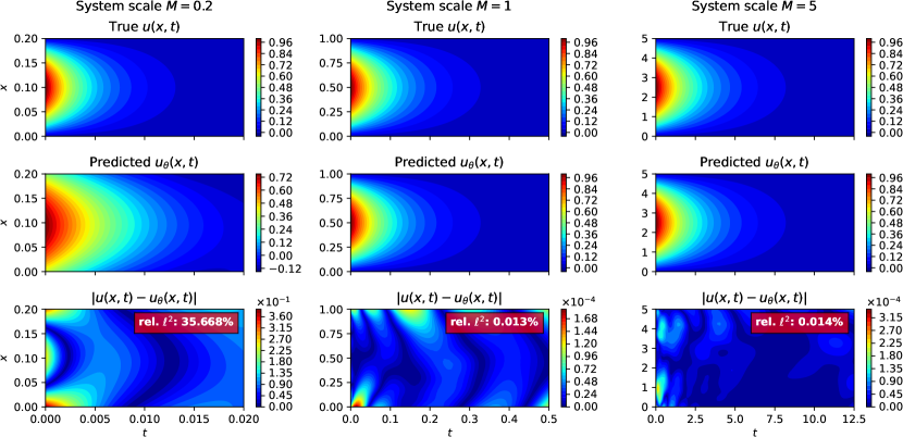
Figure 4: Heat equation. Analytical (top) and learned (mid) solution functions for $\kappa=1$ and $\alpha=0.5$. Residual error distribution (bottom) with measured relative $\ell^{2}$-errors in red boxes. Different system scales are shown column wise.

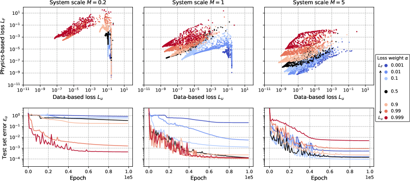
Figure 5: Heat equation. Training and test measures as intermediate steps of gradient descent optimization for diffusion coefficient $\kappa=1$. Top: data-based loss $L_{u}$ vs. physics-based loss $L_{F}$. Bottom: relative $\ell^{2}$-errors measured on the test set. Multi-objective loss function is weighted according to equation (5) and used loss weights $\alpha$ are shown as color code. Different systems scales are arranged column wise.

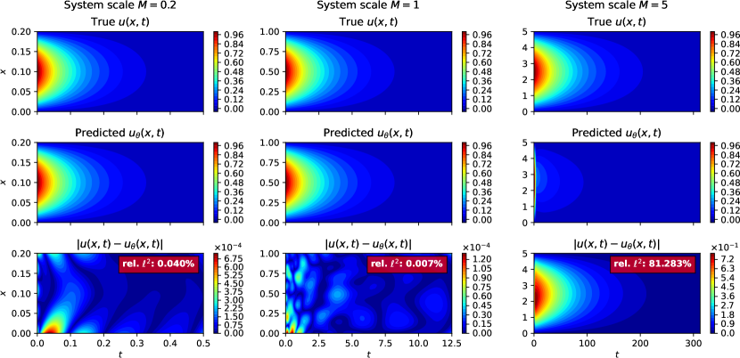
Figure 6: Heat equation. Analytical (top) and learned (mid) solution functions for $\kappa=0.04$ and $\alpha=0.5$. Residual error distribution (bottom) with measured relative $\ell^{2}$-errors in red boxes. Different system scales are shown column wise.

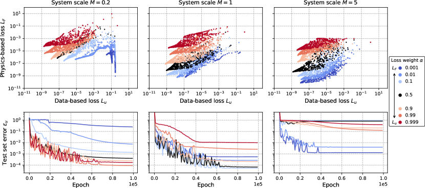
Figure 7: Heat equation. Training and test measures as intermediate steps of gradient descent optimization for $\kappa=0.04$. Top: data-based loss $L_{u}$ vs. physics-based loss $L_{F}$. Bottom: relative $\ell^{2}$-errors measured on the test set. Multi-objective loss function is weighted according to equation (5) and used loss weights $\alpha$ are shown as color code. Different systems scales are arranged column wise.

We now proceed by repeating the exact same testing procedure for a different thermal diffusivity $\kappa=0.04$. Again, we first consider the unweighted multi-objective optimization by taking $\alpha=0.5$ in the loss definition (5). The results are summarized in Figure 6 where different system scales $M=[0.2,1,5]$ are arranged column wise. The rows illustrate analytical solutions, learned solutions and residual error distributions in respective order. This time, the learned solution function for $M=0.2$ (left panel) is in good agreement with the analytical solution ($\epsilon_{u}=0.04\%$), and the model performing on $M=5$ (right panel) yields inaccurate results ($\epsilon_{u}\approx 81\%$). Similar to the previous test scenario, results for $M=1$ (middle panel) show a low relative $\ell^{2}$-error, here $\epsilon_{u}=0.007\%$.

As a next step, we adjust the loss weight $\alpha$ in the multi-objective optimization and record training and test measures as performed previously. The results are given in Figure 7 where different system scales, again, are shown column wise. From the results it is evident, that for $\kappa=0.04$ the innate shape of the Pareto front has changed compared to $\kappa=1$. The transition is more apparent for $M=0.2$ (left panel) where the previous concave shape has now changed to a shape similar of what has been observed for $M=1$ using $\kappa=1$ in Figure 5. Likewise, the shape of $M=1$ (middle panel) is now clearly convex and comparable to $M=5$ using $\kappa=1$ in Figure 5. A view on the measured relative $\ell^{2}$-errors in the second row of Figure 7, reveals further insights. Namely, the change in the course of relative $\ell^{2}$-errors, comparing the results for the different system scales using $\kappa=0.04$ and $\kappa=1$, goes along with the change in the convexity of the Pareto front. However, a yet unobserved behaviour can be seen for the system scale $M=5$ (right panel): The shape of the Pareto front can be seen as convex and measured training losses, in general, are comparatively low. Still, certain choices for the loss weight, e.g. $\alpha=0.5$, result in a large discrepancy between true and predicted solution shown by large relative $\ell^{2}$-errors. From Figure 6 we conclude that this behaviour can be explained due to network accurately learning the IC and BC, but reducing the function inside the domain to the trivial zero solution function.

Further discussion on the obtained results is provided in section 5.

4.2 Navier-Stokes and Continuity Equation

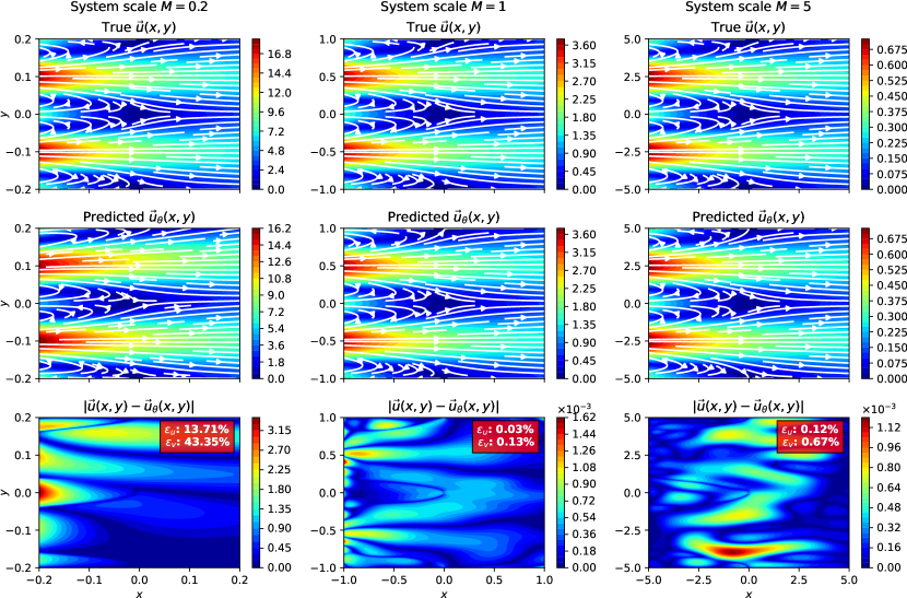
Figure 8: Navier-Stokes equations. Analytical (top) and learned (mid) solution functions for the flow field using $\nu=1/40$ and $\alpha=0.5$ in the multi-objective optimization. Color code represents the magnitude of the flow field, i.e. $\|\vec{u}(x,y)\|$. Residual error distribution (bottom) with measured relative $\ell^{2}$-errors in red boxes. Different system scales are shown column wise.

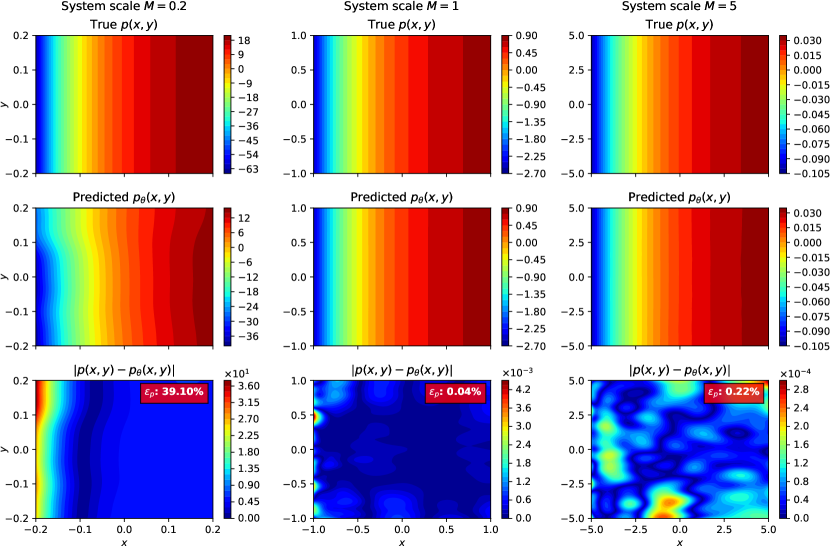
Figure 9: Navier-Stokes equations. Analytical (top) and learned (mid) solution functions for the pressure using $\nu=1/40$ and $\alpha=0.5$ in the multi-objective optimization. Residual error distribution (bottom) with measured relative $\ell^{2}$-errors in red boxes. Different system scales are shown column wise.

Figure 10: Navier-Stokes equation. Training and test measures as intermediate steps of gradient descent optimization for $\nu=1/40$. Top: data-based loss $L_{u}$ vs. physics-based loss $L_{F}$. Bottom: relative $\ell^{2}$-errors of the pressure measured on the test set. Multi-objective loss function is weighted according to equation (5) and used loss weights $\alpha$ are shown as color code. Different systems scales are arranged column wise.

To demonstrate the presence of similar observations in other problem definitions, we apply the same testing procedure on solving the Navier-Stokes equations, see section 3.2. Here, we consider a computational domain $(x,y)\in\Omega\equiv[-M,M]^{2}$ and take $\nu=1/40$, thus $Re=40$. To provide comparability for the solution of the pressure (12c), we choose the constant $C$ in a way such that the pressure has zero average on the computational domain. Similarly, we normalize the model’s prediction on the pressure to provide direct comparability to the analytical solution. Training data for the BC, collocation and the test set is sampled with sizes $N_{\mathrm{BC}}=400$, $N_{\mathrm{col}}=2500$ and $N_{\mathrm{test}}=1000$, respectively. In this specific application the range of the target values $u(x,y),v(x,y)$ and $p(x,y)$ differ for the selected system scales. As measured loss quantities and relative $\ell^{2}$-errors are sensitive to the range of the target value, a quantitative comparison between different system scales is not directly possible and should be avoided.

We first train the model by considering the unweighted multi-objective optimization using $\alpha=0.5$. The analytical and predicted solution, as well as residual errors on the flow field can be found in Figure 8. Results for the pressure are shown in Figure 9. In both figures, results for the different system scales $M=[0.2,1,5]$ are arranged as columns. Similar to what has been observed for the diffusion equation, system dynamics learned by the PINN strongly differ when performing the computation on different system scales. For $M=1$ (middle panel) and $M=5$ (right panel) the PINN’s prediction is in good agreement with the analytical solution (measured relative $\ell^{2}$-errors are below $0.7\%$). For $M=0.2$ (left panel) large prediction errors are measured: here relative $\ell^{2}$-errors are greater than $13\%$.

To further analyze the multi-objective optimization, we proceed by training the model with different loss weights $\alpha$. Results for this test are shown in Figure 10. The first row shows the data-based loss $L_{u}$ plotted against the physics-based loss $L_{F}$ as intermediate steps of the gradient descent optimization. In the second row the relative $\ell^{2}$-error of the predicted pressure $\epsilon_{p}$ on the test set is plotted as the main performance measure for this application. Since we observe that the PINN’s accuracy on the predicted flow velocities is similar to that of the pressure, the display of their relative $\ell^{2}$-errors is omitted for clarity. From Figure 10 it is apparent that Pareto optima obtained on the system scale $M=0.2$ (left panel) are influenced by the concave shape of the Pareto front. As a result, the unweighted multi-objective optimization ($\alpha=0.5$), shown in Figure 8 and 9, converges to a Pareto optimum where learned system dynamics are inaccurate. In this case, greater loss weights on the data-based loss, i.e. $\alpha\to 1$, yield lower training losses and predicted solutions are in better agreement with the analytical solution. For the system scale $M=5$ (right panel) the Pareto front is clearly convex and, in general, a greater loss weight on the physics-based loss, i.e. $\alpha\to 0$, results in low measured relative $\ell^{2}$-errors. The system scale $M=1$ (middle panel) is an intermediate trend of both for which the unweighted multi-objective optimization converges to an acceptable Pareto optimum with correctly learned system dynamics.

In general, the obtained results demonstrate a notable effect of the used system scale on the multi-objective optimization, as already observed for the previous test scenario using the diffusion equation.

4.3 Adaptive Activation Function and Adaptive Loss Weighting

Figure 11: Heat equation. Training and test measures as intermediate steps of gradient descent optimization for diffusion coefficient $\kappa=1$. Top: data-based loss $L_{u}$ vs. physics-based loss $L_{F}$. Bottom: relative $\ell^{2}$-errors measured on the test set. Highlighted curves (green and orange) are obtained when using an adaptive activation function (AF) and adaptive loss weighting (LW) in the training process. The unweighted multi-objective optimization, i.e. $\alpha=0.5$, is shown as blue trajectory. Different systems scales are arranged column wise.

For the following and final tests, we focus on two specific variants in training the PINN: the use of state-of-the-art adaptive activation functions [27, 28] and adaptive loss weighting methods [21, 26]. Both variants were proposed in the context of PINNs and, in general, should provide better convergence properties. Former introduce a trainable variable in the neural network activation function which changes dynamically the topology of the loss function during model training. Latter, on the other hand, use an adaptive update scheme for the loss weights by means of back-propagated gradients. For a detailed discussion of both variants, the reader is referred to reference [27] and [21].

To investigate the effectiveness of the two variants, we again study the heat equation with $\kappa=1$, but train the PINN once by using (i) a global adaptive activation function with the hyperbolic tangent and scale factor $n=5$ and (ii) adaptive loss weighting with the mean of back-propagated gradients according to reference [26]. For the test run using the adaptive activation, the loss weight is set to $\alpha=0.5$.

The results are summarized in Figure 11 as highlighted trajectories (green and orange). For comparability, the unweighted multi-objective optimization ($\alpha=0.5$) using neither variants is shown in blue. The adaptive activation function seems to only provide moderate improvement in the accuracy and model convergence for the system scale $M=0.2$. The adaptive loss weighting, on the other hand, performs well on any system scale and chooses an effective trading between data- and physics-based loss. Further analysis and discussion on the obtained results are provided in the next section.

5 Discussion

5.1 The Pareto Front in Physics-Informed Neural Networks

In the multi-objective context of PINNs, the importance of a loss weight that trades between data and physics-based loss has been discussed several times in literature and verified in this study. We use a weighted linear combination of the two losses, see equation (5), to analyse the multi-objective optimization when solving the (i) diffusion equation and (ii) Navier-Stokes Equations. A representative sample of the loss weight $\alpha$, see Figure 5, 7 and 10, shows that more accurate results can be obtained when either data- or physics-based loss is weighted greater than the other. The accuracy, in this context, is measured by the relative $\ell^{2}$-error on a test set after optimized and full model training. Whether or not a suitable loss weight leads to correct system dynamics is strongly influenced by the innate shape of the Pareto front, also visible in Figure 5, 7 and 10. For some system settings, see Figure 5 and  10, the collection of Pareto optima follows a concave shape of the Pareto front. In general, the concave Pareto front lets the user decide which of strongly dominating optima is chosen by adjusting the loss weight $\alpha$. By analysing the corresponding errors on the set, we observe that at least one of the optima, here specified through $\alpha\to 1$, is in good agreement with the true system dynamics. Other optima, i.e. $\alpha\to 0$, suffer from a yet unsolved conflict between the losses, which we relate to the frequently reported convergence issues of PINNs.

The shape of the Pareto front, in general, is influenced by different causes like model-specific parameters (network architecture, activation function), the definition of individual loss terms and system parameters. Since we keep the design choices and loss definitions fixed, we effectively isolate the role of system parameters on the shape of the Pareto front.

5.2 On the Role of System Parameters in the Multi-objective Optimization

In this work, we did not try to find a suitable choice of system parameters, but rather we investigate how human choices of system parameters can affect convergence properties of PINNs. We use a standard definition of the PINN optimization and our results clearly show that convergence properties strongly depend on the used system scale specified by the computational domain. For some system settings, see Figure 4, 6, 8 and 9, the unweighted linear combination of data- and physics-based loss leads to inaccurate results, measured by a large relative $\ell^{2}$-error on the test set. Those results demonstrate inconsistent PINN convergence and accuracy when given one and the same system dynamics at different system scales. Selecting a suitable system scale, e.g a non-dimensionalized form, thus is crucial in obtaining accurate results when using PINNs for solving foward and inverse problems governed by PDEs.

It is to be expected that the relation of individual system dimensions in two- or higher-dimensional problems can have a certain influence on the convergence of PINNs. Problems in which one system dimension dominates the others can be related to this specific case. As a concrete example in literature, we refer to reference [7] in which convergences issues were reported when using a PINN with soft constraints for solving the two-dimensional channel flow. Complex geometries which are inherent to the system under study, thus, may be challenging for setting up a well-working application.

Further, we find that the parametrization of the governing PDE influences the convergence properties. Comparing Figure 4 and 6, it is clearly evident that the choice of the parametrization coefficient, here the thermal diffusivity, affects the multi-objective optimization and convergence of the PINN.

Comparing the results for the diffusion equation, it is evident from Figure 5 and 7 that similar shapes of the Pareto front are observed when a certain relationship of the system parameters are encountered. In this specific problem, we use the diffusive times scale $T=M^{2}/\kappa$ as characteristic system dimension and, from the figures, it is apparent that the Pareto front of different system scales coincides for similar values of $T$. As an explanation to these observations, we refer to the relationship of partial derivatives and thermal diffusivity as they appear in the definition of the heat equation (6). It seems that given system dimensions and PDE parametrizations influence the way how the multi-objective optimization minimizes the data- and physics-based loss. If the system parameters are well-chosen, the multi-objective optimization may find an easy way to reduce the constituent losses. In this case a convex shape of the Pareto front can be observed and any chosen loss weight leads to accurate predictions. Other system parameters potentially complicate the multi-objective optimization which results in a concave shape of the Pareto front. Due to the simplicity of the heat equation and the well-studied problem definition, we could introduce the characteristic time scale and manage to obtain the clear results. For other, more complex sets of PDEs, e.g. the Navier-Stokes equations, such an approach may be difficult or even elusive.

5.3 Possible Approaches for Improved Convergence Properties

From our results in Figure 5, 7 and 10 it is evident that the PINN performing on the system scale $M=1$ shows well-behaved training properties. Major part of the Pareto front on those examples is convex and the simple unweighted multi-objective optimization does indeed converge to an accurate solution. This is not surprising as the system scale $M=1$ relates to the non-dimensionalized form of the systems being studied. From these observations we conclude that a properly performed non-dimensionalization helps PINNs in learning correct system dynamics without additional adjustments in the multi-objective optimization. The non-dimensionalization, however, can be cumbersome and dimensionless variables chosen freely by the user for a given problem. Sometimes the statement of the problem gives hints, e.g. on the physical length or time scale of the system. Often, the problem has to be solved first and the notation simplified by looking at the solution. This approach may be elaborate or even elusive for some application where one eventually ends up with a partial removal of system dimensions.

Figure 11 demonstrates the effectiveness of a state-of-the-art adaptive activation function and adaptive loss weighting method. The results show that the adaptive activation function provides moderate improvement for a specific system scale, but rather fails at others. This is interesting, as the adaptive activation function does not change the expressive power of the PINN: any learned scaling factor in the global adaptive activation function can also be implemented by a joint scaling of the incoming weights of the preceding layer. However, this additional degree of freedom changes the optimization landscape and, thus, influences the trajectory of the optimization. Different scaling factors $n$, locally defined activation functions, or a combined use of weighted multi-objective optimization may improve the effectiveness of this modification. The adaptive loss weighting, however, performs well and shows an effective trading between data- and physics-based loss on any given system scale. This potentially reduces the need for manually tuned loss weights. Still, the multi-objective convergence of both investigated variants is determined by the innate shape of the Pareto front, as visible in the figure.

Finally, a possible approach to circumvent the multi-objectiveness and occurring convergence issues is the encoding of hard constraints, e.g. for initial or boundary conditions. Reference [41] demonstrated the effective use of hard initial/boundary constraints in complex geometries which was later applied on the channel flow [7].

6 Conclusion

Physics-informed neural networks (PINNs) have gained high attention when tackling forward and inverse problems involving partial differential equations. Their accuracy on a specific task usually cannot be determined in advance and convergence issues still remain a vague issue. When using PINNs with a data- and physics-based loss, minimized through multi-objective optimization, the use of loss weights is crucial. This, we could verify by solving the (i) diffusion equation and (ii) Navier-Stokes equations while using different system parameters. Our results have also shown that the multi-objective optimization in PINNs is strongly affected by the innate shape of the Pareto front. We could qualitatively demonstrate that the shape of the Pareto front is determined by the parameters of governing differential equations and the absolute scale of the system under study (i.e. by the parameters of the computational domain). Furthermore, we could observe that state-of-the-art variants of PINNs, including adaptive activation functions and adaptive loss weight methods, are also influenced by the shape of the Pareto front. However, since these adaptations affect the loss landscape for the optimization algorithm, they were shown to have moderate positive effects on the convergence of PINNs. Future work will investigate techniques for reparametrizing the network architectures and/or the problems under study to appropriately shape the Pareto front, and whether established techniques for multi-objective optimization such as [25] can also be applied to the PINN setting. In summary, the results have demonstrated the prominent role of the system parameters in the multi-objective optimization of PINNs.

References

- [1] Balázs Csanád Csáji et al. Approximation with artificial neural networks. Faculty of Sciences, Etvs Lornd University, Hungary, 24(48):7, 2001.
- [2] Zhou Lu, Hongming Pu, Feicheng Wang, Zhiqiang Hu, and Liwei Wang. The expressive power of neural networks: A view from the width. arXiv preprint arXiv:1709.02540, 2017.
- [3] Kaiming He, Xiangyu Zhang, Shaoqing Ren, and Jian Sun. Deep residual learning for image recognition. In Proceedings of the IEEE conference on computer vision and pattern recognition, pages 770–778, 2016.
- [4] John Lafferty, Andrew McCallum, and Fernando CN Pereira. Conditional random fields: Probabilistic models for segmenting and labeling sequence data. 2001.
- [5] Ian J Goodfellow, Jean Pouget-Abadie, Mehdi Mirza, Bing Xu, David Warde-Farley, Sherjil Ozair, Aaron Courville, and Yoshua Bengio. Generative adversarial networks. arXiv preprint arXiv:1406.2661, 2014.
- [6] Maziar Raissi, Alireza Yazdani, and George Em Karniadakis. Hidden fluid mechanics: Learning velocity and pressure fields from flow visualizations. Science, 367(6481):1026–1030, 2020.
- [7] Luning Sun, Han Gao, Shaowu Pan, and Jian-Xun Wang. Surrogate modeling for fluid flows based on physics-constrained deep learning without simulation data. Computer Methods in Applied Mechanics and Engineering, 361:112732, 2020.
- [8] Yuyao Chen, Lu Lu, George Em Karniadakis, and Luca Dal Negro. Physics-informed neural networks for inverse problems in nano-optics and metamaterials. Optics express, 28(8):11618–11633, 2020.
- [9] Francisco Sahli Costabal, Yibo Yang, Paris Perdikaris, Daniel E Hurtado, and Ellen Kuhl. Physics-informed neural networks for cardiac activation mapping. Frontiers in Physics, 8:42, 2020.
- [10] Georgios Kissas, Yibo Yang, Eileen Hwuang, Walter R Witschey, John A Detre, and Paris Perdikaris. Machine learning in cardiovascular flows modeling: Predicting arterial blood pressure from non-invasive 4d flow mri data using physics-informed neural networks. Computer Methods in Applied Mechanics and Engineering, 358:112623, 2020.
- [11] Zhiping Mao, Ameya D Jagtap, and George Em Karniadakis. Physics-informed neural networks for high-speed flows. Computer Methods in Applied Mechanics and Engineering, 360:112789, 2020.
- [12] Arinan Dourado and Felipe AC Viana. Physics-informed neural networks for missing physics estimation in cumulative damage models: a case study in corrosion fatigue. Journal of Computing and Information Science in Engineering, 20(6), 2020.
- [13] QiZhi He, David Barajas-Solano, Guzel Tartakovsky, and Alexandre M Tartakovsky. Physics-informed neural networks for multiphysics data assimilation with application to subsurface transport. Advances in Water Resources, 141:103610, 2020.
- [14] Minglang Yin, Xiaoning Zheng, Jay D Humphrey, and George Em Karniadakis. Non-invasive inference of thrombus material properties with physics-informed neural networks. Computer Methods in Applied Mechanics and Engineering, 375:113603, 2021.
- [15] Isaac E Lagaris, Aristidis Likas, and Dimitrios I Fotiadis. Artificial neural networks for solving ordinary and partial differential equations. IEEE transactions on neural networks, 9(5):987–1000, 1998.
- [16] Maziar Raissi, Paris Perdikaris, and George E Karniadakis. Physics-informed neural networks: A deep learning framework for solving forward and inverse problems involving nonlinear partial differential equations. Journal of Computational Physics, 378:686–707, 2019.
- [17] Ehsan Haghighat, Maziar Raissi, Adrian Moure, Hector Gomez, and Ruben Juanes. A physics-informed deep learning framework for inversion and surrogate modeling in solid mechanics. Computer Methods in Applied Mechanics and Engineering, 379:113741, 2021.
- [18] XIA Yang, Suhaib Zafar, J-X Wang, and Heng Xiao. Predictive large-eddy-simulation wall modeling via physics-informed neural networks. Physical Review Fluids, 4(3):034602, 2019.
- [19] Liu Yang, Xuhui Meng, and George Em Karniadakis. B-pinns: Bayesian physics-informed neural networks for forward and inverse pde problems with noisy data. Journal of Computational Physics, 425:109913, 2021.
- [20] Teeratorn Kadeethum, Thomas M Jørgensen, Hamidreza M Nick, et al. Physics-informed neural networks for solving inverse problems of nonlinear biot’s equations: Batch training. In 54th US Rock Mechanics/Geomechanics Symposium. American Rock Mechanics Association, 2020.
- [21] Sifan Wang, Yujun Teng, and Paris Perdikaris. Understanding and mitigating gradient pathologies in physics-informed neural networks. arXiv preprint arXiv:2001.04536, 2020.
- [22] Olga Fuks and Hamdi A Tchelepi. Limitations of physics informed machine learning for nonlinear two-phase transport in porous media. Journal of Machine Learning for Modeling and Computing, 1(1), 2020.
- [23] Sifan Wang, Xinling Yu, and Paris Perdikaris. When and why pinns fail to train: A neural tangent kernel perspective. arXiv preprint arXiv:2007.14527, 2020.
- [24] C-L Hwang and Abu Syed Md Masud. Multiple objective decision making—methods and applications: a state-of-the-art survey, volume 164. Springer Science & Business Media, 2012.
- [25] John C Platt and Alan H Barr. Constrained differential optimization for neural networks. 1988.
- [26] Xiaowei Jin, Shengze Cai, Hui Li, and George Em Karniadakis. Nsfnets (navier-stokes flow nets): Physics-informed neural networks for the incompressible navier-stokes equations. Journal of Computational Physics, 426:109951, 2021.
- [27] Ameya D Jagtap, Kenji Kawaguchi, and George Em Karniadakis. Adaptive activation functions accelerate convergence in deep and physics-informed neural networks. Journal of Computational Physics, 404:109136, 2020.
- [28] Ameya D Jagtap, Kenji Kawaguchi, and George Em Karniadakis. Locally adaptive activation functions with slope recovery for deep and physics-informed neural networks. Proceedings of the Royal Society A, 476(2239):20200334, 2020.
- [29] Yibo Yang and Paris Perdikaris. Adversarial uncertainty quantification in physics-informed neural networks. Journal of Computational Physics, 394:136–152, 2019.
- [30] Dongkun Zhang, Lu Lu, Ling Guo, and George Em Karniadakis. Quantifying total uncertainty in physics-informed neural networks for solving forward and inverse stochastic problems. Journal of Computational Physics, 397:108850, 2019.
- [31] Hao Li, Zheng Xu, Gavin Taylor, Christoph Studer, and Tom Goldstein. Visualizing the loss landscape of neural nets. arXiv preprint arXiv:1712.09913, 2017.
- [32] Atilim Gunes Baydin, Barak A Pearlmutter, Alexey Andreyevich Radul, and Jeffrey Mark Siskind. Automatic differentiation in machine learning: a survey. Journal of machine learning research, 18, 2018.
- [33] Martín Abadi, Ashish Agarwal, Paul Barham, Eugene Brevdo, Zhifeng Chen, Craig Citro, Greg S Corrado, Andy Davis, Jeffrey Dean, Matthieu Devin, et al. Tensorflow: Large-scale machine learning on heterogeneous distributed systems. arXiv preprint arXiv:1603.04467, 2016.
- [34] Adam Paszke, Sam Gross, Soumith Chintala, Gregory Chanan, Edward Yang, Zachary DeVito, Zeming Lin, Alban Desmaison, Luca Antiga, and Adam Lerer. Automatic differentiation in pytorch. 2017.
- [35] Mohammad Amin Nabian, Rini Jasmine Gladstone, and Hadi Meidani. Efficient training of physics-informed neural networks via importance sampling. Computer-Aided Civil and Infrastructure Engineering, 2021.
- [36] Colby L Wight and Jia Zhao. Solving allen-cahn and cahn-hilliard equations using the adaptive physics informed neural networks. arXiv preprint arXiv:2007.04542, 2020.
- [37] Christopher J Arthurs and Andrew P King. Active training of physics-informed neural networks to aggregate and interpolate parametric solutions to the navier-stokes equations. Journal of Computational Physics, page 110364, 2021.
- [38] LIG Kovasznay. Laminar flow behind a two-dimensional grid. In Mathematical Proceedings of the Cambridge Philosophical Society, volume 44, pages 58–62. Cambridge University Press, 1948.
- [39] Diederik P Kingma and Jimmy Ba. Adam: A method for stochastic optimization. arXiv preprint arXiv:1412.6980, 2014.
- [40] Xavier Glorot and Yoshua Bengio. Understanding the difficulty of training deep feedforward neural networks. In Proceedings of the thirteenth international conference on artificial intelligence and statistics, pages 249–256. JMLR Workshop and Conference Proceedings, 2010.
- [41] Jens Berg and Kaj Nyström. A unified deep artificial neural network approach to partial differential equations in complex geometries. Neurocomputing, 317:28–41, 2018.