Transfer Learning on Multi-Fidelity Data

Abstract

Neural networks (NNs) are often used as surrogates or emulators of partial differential equations (PDEs) that describe the dynamics of complex systems. A virtually negligible computational cost of such surrogates renders them an attractive tool for ensemble-based computation, which requires a large number of repeated PDE solves. Since the latter are also needed to generate sufficient data for NN training, the usefulness of NN-based surrogates hinges on the balance between the training cost and the computational gain stemming from their deployment. We rely on multi-fidelity simulations to reduce the cost of data generation for subsequent training of a deep convolutional NN (CNN) using transfer learning. High- and low-fidelity images are generated by solving PDEs on fine and coarse meshes, respectively. We use theoretical results for multilevel Monte Carlo to guide our choice of the numbers of images of each kind. We demonstrate the performance of this multi-fidelity training strategy on the problem of estimation of the distribution of a quantity of interest, whose dynamics is governed by a system of nonlinear PDEs (parabolic PDEs of multi-phase flow in heterogeneous porous media) with uncertain/random parameters. Our numerical experiments demonstrate that a mixture of a comparatively large number of low-fidelity data and smaller numbers of high- and low-fidelity data provides an optimal balance of computational speed-up and prediction accuracy. The former is reported relative to both CNN training on high-fidelity images only and Monte Carlo solution of the PDEs. The latter is expressed in terms of both the Wasserstein distance and the Kullback–Leibler divergence.

1 Introduction

Machine learning techniques, especially neural networks (NNs), have pervaded every facet of human activity and has permeated into the field of scientific computing. In the latter setting, NNs are used to approximate highly nonlinear and irregular functions (Friedman et al., 2001), solve (ordinary and partial) differential equations (e.g., Lee and Kang, 1990; Lagaris et al., 1998; Fuks and Tchelepi, 2020, among many others), and construct cheap surrogates for ensemble-based computation (e.g., Mo et al., 2019a; Raissi et al., 2019). Examples of the latter include inverse modeling (Mo et al., 2019b; Zhou and Tartakovsky, 2021), data assimilation (Tang et al., 2020), and uncertainty quantification (Tripathy and Bilionis, 2018; Zhu et al., 2019).

A typical ensemble-based computation of practical significance involves repeated solves of (coupled, nonlinear) partial-differential equations (PDEs)

$$\mathcal{N}(\mathbf{u};\bm{\theta})=g(\mathbf{x},t;\bm{\theta}),\qquad(\mathbf{x},t)\in D\times(0,T],$$ (1)

which describe the spatiotemporal evolution of (a set of) state variables $\mathbf{u}(\mathbf{x},t)$ in the computational domain $D$ over simulation time horizon $(0,T]$. Multiple solves of (1)—for different values of the inputs $\bm{\theta}(\mathbf{x},t)$ that parameterize the differential operator $\mathcal{N}$, the source function $g$, and auxiliary functions in the initial and/or boundary conditions—are required because these values are known at best in terms of their distributions, which are either inferred from data or provided by the expert. High computational cost of solving (1) numerically often precludes one from generating enough samples to obtain meaningful statistics of $\mathbf{u}(\mathbf{x},t)$ or the derived quantities of interest. A surrogate of (1) carries a negligible cost, making possible ensemble-based computation with arbitrarily small sampling error.

Alternative strategies for surrogate construction include polynomial chaos expansions (Xiu, 2010), Kriging or Gaussian processes (Couckuyt et al., 2014), polynomial regression (Montgomery and Evans, 2018), tensor-product splines (Hwang and Martins, 2018) and random forests (Breiman, 2001). Current popularity of NN-based surrogates (Mo et al., 2019a; Raissi et al., 2019) is grounded in the scalability and approximation capabilities of deep NNs (Friedman et al., 2001; Tripathy and Bilionis, 2018). Regardless of the surrogate type, the training of a surrogate requires a large number of solves of (1) for different combinations of parameter values $\bm{\theta}$. Advanced computer architectures, e.g., CUDA-compatible graphics processing units (GPUs) and tensor processing units (TPUs), are almost a necessity to train a large NN. A combined cost of training-data acquisition and NN training can be so large as to negate the benefits of the NN.

This observation suggests that the practical utility of a NN as a surrogate model hinges on one’s ability to dramatically reduce the cost of its construction. We rely on multi-fidelity simulations to reduce the cost of data generation for subsequent training of a deep convolutional NN (CNN) using transfer learning. High- and low-fidelity images are generated by solving PDE (1) on fine and coarse meshes, respectively. A fine mesh is defined by the need to resolve the spatiotemporal variability of the model’s inputs $\bm{\theta}$ and outputs $\mathbf{u}$; the resulting high-fidelity simulation carries a high computational cost. Lower-fidelity solutions of (1), obtained on coarser meshes on which appropriately homogenized inputs $\bm{\theta}_{\text{hom}}$ are defined, are cheaper to compute but less accurate. We train a CNN on a mixture of these multi-fidelity data, using the theoretical results for multilevel Monte Carlo (MLMC) (Heinrich, 1998, 2001; Giles, 2008; Taverniers et al., 2020) to guide our choice of the numbers of solutions $\mathbf{u}(\mathbf{x},t)$ of each kind. Similar to MLMC (Müller et al., 2013; Peherstorfer, 2019), the varying fidelity (aka “levels”) of predictions of $\mathbf{u}$ can be achieved not only by solving (1) on different meshes, but also by replacing (1) with its cheaper-to-compute counterparts. For example, the multi-phase flow equations used as the computational testbed in this study can be replaced with the cheaper-to-solve Richards equation and Green-Ampt equation (Yang et al., 2020; Sinsbeck and Tartakovsky, 2015), each of which encapsulates progressively simplified physics. We leave this aspect of NN training on multi-fidelity data for a follow-up study.

Section 2 contains a brief description of our CNN and the workflow for its training on multi-fidelity of data. The performance of this algorithm is tested on a system of nonlinear parabolic PDEs governing multi-phase flow in a heterogeneous porous medium with uncertain properties, which are formulated in Section 3. In Section 4, we demonstrate the accuracy and computational efficiency of the CNN-based surrogate used to quantify predictive uncertainty of (1) in terms of the distribution of a quantity of interest. Main conclusions drawn from this study are presented in Section 5.

2 Deep Convolutional Neural Networks

While many flavors of NNs can be used as a surrogate for a PDE-based model like (1), we choose CNNs because of their proven ability to model complex nonlinear phenomena and the negligible cost of their forward pass. To be concrete, we select the CNN with encoder-decoder architecture (Mo et al., 2019b), which has previously been used for single-phase (Mo et al., 2019a) and multi-phase (Mo et al., 2019b) flow problems in the context of uncertainty quantification. The encoder-decoder architecture is ideally suited for training on multi-fidelity data, as detailed in Section 2.1.

The CNN-based surrogate is set up as an image-to-image regression model (Zhou and Tartakovsky, 2021). To train and test the network, we use the parameter values $\bm{\theta}(\mathbf{x}_{i})$ in $N_{\text{el}}$ elements $\{\mathbf{x}_{i}\}_{i=1}^{N_{\text{el}}}$ of a numerical grid as input and the discretized solution $\mathbf{u}(\mathbf{x}_{i},t_{k})$ of PDE (1) at $N_{\text{ts}}$ time steps $\{t_{k}\}_{k=1}^{N_{\text{ts}}}$ as output. To facilitate the generalizibility of the trained CNN to unseen sets of the input $\bm{\theta}(\mathbf{x}_{i})$, i.e., to ensure that the CNN is not over-fitted to a particular choice of $\bm{\theta}(\mathbf{x}_{i})$, the training data comprises a large number $N_{\text{train}}$ of the solutions $\mathbf{u}$ obtained for $N_{\text{train}}$ realizations $\{\bm{\theta}_{1},\dots,\bm{\theta}_{N_{\text{train}}}\}$ of the input $\bm{\theta}$. The loss function,

$$\mathcal{L}(\mathbf{w})=\sum_{m=1}^{N_{\text{train}}}\sum_{i=1}^{N_{\text{el}}}\sum_{k=1}^{N_{\text{ts}}}|\mathbf{u}(\mathbf{x}_{i},t_{k};\bm{\theta}_{m})-\hat{\mathbf{u}}_{ik}(\mathbf{w};\bm{\theta}_{m})|+\lambda\sum_{n=1}^{N_{\text{w}}}w_{n}^{2}$$ (2)

consists of two parts. The first represents the $L_{1}$-norm discrepancy between the state variables $\mathbf{u}$ predicted by solving PDE (1), $\mathbf{u}(\mathbf{x}_{i},t_{k})$ and estimated by the CNN, $\hat{\mathbf{u}}_{ik}(\mathbf{w})$, with $N_{\text{w}}$ weights $\mathbf{w}=(w_{1},\dots,w_{N_{\text{w}}})^{\top}$. The $L_{2}$-norm regularization term prevents over-fitting by penalizing large weights $\mathbf{w}$ associated complex models; the regularization parameter $\lambda$ determines how much regularization penalty is applied. The CNN training consists of finding a set of weights $\mathbf{w}^{\star}$ that minimizes $\mathcal{L}$.

2.1 Transfer Learning

The construction of CNN-based generalizable surrogates, which are capable of making predictions for realizations of $\bm{\theta}(\mathbf{x})$ not seen during training, requires a large number of PDE solves, $N_{\text{train}}$; e.g., $N_{\text{train}}\sim 1500$ was used by Mo et al. (2019a) and Zhou and Tartakovsky (2021) to train the encoder-decoder CNNs similar to ours. If a single PDE solve is expensive, the costs associate with large $N_{\text{train}}$ can be large to the point where CNN training becomes unfeasible. To alleviate this problem, we use both multi-fidelity data and transfer learning (Donahue et al., 2014). The latter is a technique that uses a NN trained for one task as the starting point for a different NN being trained for a new task. Transfer learning has been implemented for face detection (Jiang and Learned-Miller, 2017), generation of image description (Karpathy and Fei-Fei, 2015), and construction of physics-informed NNs (Haghighat et al., 2021), among other applications.

Let HFS and LFS data refer to the solutions of (1), $\mathbf{u}(\mathbf{x}_{i},t_{k})$, obtained on the fine ($N_{\text{el}}=N_{\text{el}}^{\text{HFS}}$) and coarse ($N_{\text{el}}=N_{\text{el}}^{\text{LFS}}$ with $N_{\text{el}}^{\text{LFS}}<N_{\text{el}}^{\text{HFS}}$) meshes, respectively. If $N_{\text{w}}$ in (2) denotes the number of weights in the CNN trained on the HFS data, then our implementation of transfer learning starts with the construction of a CNN composed of $N_{\text{LFS}}$ ($N_{\text{LFS}}<N_{\text{w}}$) weights $\mathbf{w}_{\text{LFS}}=(w_{1},\dots,w_{N_{\text{LFS}}})^{\top}$ trained on the LFS data. Then, the HFS data are used to train the desired high-resolution CNN, i.e., to determine the remaining weights $\mathbf{w}_{\text{HFS}}=(w_{N_{\text{LFS}}+1},\dots,w_{N_{\text{w}}})^{\top}$. This transfer learning strategy is depicted in Fig. 1 and detailed below.

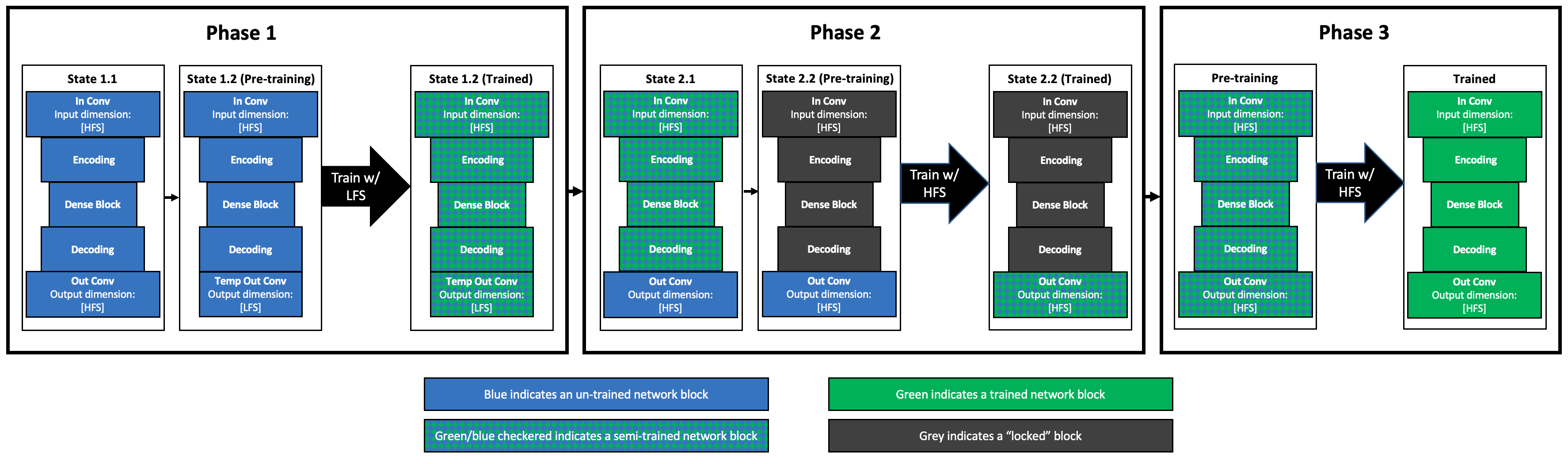
Figure 1: Workflow for CNN training on multi-fidelity data. Phase 1 returns a low-resolution CNN trained on the LFS data. Phase 2 supplements that network with an additional layer whose weights are determined from the HFS data, producing a high-resolution CNN. In Phase 3, the latter is fine-tuned by allowing all the weights to vary during the training on the same HFS data. LABEL:appendix:_A provides a pseudocode for all three Phases.

2.2 Workflow for CNN Training on Multi-fidelity Data

Our strategy for CNN training on multi-fidelity data consists of three phases (Fig. 1), each of which results in a CNN denoted by $M_{i}$ ($i=1,2,3$). During Phase 1, the CNN $M_{1}$ with the $N_{\text{el}}^{\text{LFS}}\times N_{\text{el}}^{\text{LFS}}$ output is trained on the LFS data. In Phase 2, the CNN $M_{2}$ with $N_{\text{el}}^{\text{HFS}}\times N_{\text{el}}^{\text{HFS}}$ output is constructed by adding an additional layer with the weights $\mathbf{w}_{\text{HFS}}$, which are trained on the HFS data while keeping the original weights $\mathbf{w}_{\text{LFS}}$ fixed. Phase 3 consists of fine-tuning the CNN $M_{2}$ by allowing all the weights $\mathbf{w}=\{\mathbf{w}_{\text{LFS}},\mathbf{w}_{\text{HFS}}\}$ to update during the training on the same HFS data. The numerical experiments reported in Sections 3 and 4 demonstrate that this transfer learning strategy significantly reduces the number of high-resolution PDE solves.

The workflow of our approach is provided below (see LABEL:appendix:_A for the corresponding pseudocode).

1. Train a CNN $M_{1}$, with $N_{\text{el}}^{\text{LFS}}\times N_{\text{el}}^{\text{LFS}}$ output, on the LFS data.

   1. Initialize the transfer learning by employing the encoder-decoder CNN of Mo et al. (2019b), $M_{\text{init}}$ with $N_{\text{el}}^{\text{HFS}}\times N_{\text{el}}^{\text{HFS}}$ output, whose $N_{\text{w}}$ weights $\mathbf{w}$ are set to PyTorch defaults.

   2. Train the CNN $M_{1}$ on the LFS data. The starting point is a CNN obtained from $M_{\text{init}}$ by replacing its last layer $L_{\text{last}}$, which has $N_{\text{HFS}}$ weights $\mathbf{w}_{\text{HFS}}$, with a temporary convolution layer $L_{\text{temp}}$. The latter makes the output of $M_{1}$ match the dimensions of the LFS data, $[N_{\text{ts}}\times N_{\text{el}}^{\text{LFS}}\times N_{\text{el}}^{\text{LFS}}]$, and has significantly fewer weights than has $L_{\text{last}}$. Then, $N_{\text{LFS}}$ weights $\mathbf{w}_{\text{LFS}}$ are updated by minimizing (2) on the LFS data.

2. Train a CNN $M_{2}$, with $N_{\text{w}}$ weights $\mathbf{w}=\{\mathbf{w}_{\text{LFS}},\mathbf{w}_{\text{HFS}}\}$ (of which $N_{\text{LFS}}$ weights are locked) and $N_{\text{el}}^{\text{HFS}}\times N_{\text{el}}^{\text{HFS}}$ output, on the HFS data

   1. Build a CNN from $M_{1}$ by replacing its layer $L_{\text{temp}}$ with the layer $L_{\text{last}}$.

   2. Train the resulting CNN $M_{2}$ on the HFS data by minimizing (2) over the weights $\mathbf{w}_{\text{HFS}}$ of layer $L_{\text{last}}$, while keeping the remaining weights $\mathbf{w}_{\text{LFS}}$ fixed at their values in $M_{1}$.

3. Train a CNN $M_{3}$ on the HFS data by allowing all weights $\mathbf{w}$ of $M_{2}$ to vary during the minimization

Since the bulk of the CNN $M_{3}$ training is carried out on the LFS data, this procedure is more efficient than CNN training solely on HFS data.

3 Computational Example: Multi-phase Flow

Numerical solution of problems involving multi-phase flow in porous media is notoriously difficult because of the high degree of nonlinearity and stiffness of the governing PDEs. Each forward solve of these PDEs is so expensive that it is uncommon, e.g., in petroleum engineering, to base uncertainty quantification efforts on as few as three model runs. This high cost and numerical complexity make the multi-phase flow equations a challenging testbed for ensemble-based simulations.

We consider horizontal flow of two incompressible and immiscible fluids, with viscosities $\mu_{1}$ and $\mu_{2}$, in a heterogeneous, incompressible, and isotropic porous medium $D$. The latter is characterized by porosity $\phi$ and intrinsic permeability $k$. The porosity is assumed to be constant $\phi=0.25$, and intrinsic permeability $k(\mathbf{x})$ is treated as a random variable. Mass conservation of the $\ell$th fluid phase ($\ell=1,2$) implies

$$\phi\frac{\partial S_{\ell}}{\partial t}+\nabla\cdot\mathbf{v}_{\ell}+q_{\ell}=0,\qquad\mathbf{x}\equiv(x_{1},x_{2})^{\top}\in D,\quad t\in[0,T],$$ (3a)

where $$S_{\ell}(\mathbf{x},t) S_{1}+S_{2}=1 q_{\ell} \mathbf{v}_{\ell}(\mathbf{x},t)$$ is the phase saturation constrained by ; is the source/sink term; and the macroscopic velocity is described by the generalized Darcy law

$$\mathbf{v}_{\ell}=-k\frac{k_{r\ell}}{\mu_{\ell}}\nabla P_{\ell}.$$ (3b)

The relative permeability for the $\ell$th phase, $k_{r\ell}$, varies with the phase saturation, $k_{r\ell}=k_{r\ell}(S_{\ell})$, in accordance with the Brooks-Corey constitutive model (Corey, 1954). Following Taverniers et al. (2020) and many others, we neglect the capillary forces, i.e., assume pressure within the two phases to be equal, $P_{1}=P_{2}\equiv P(\mathbf{x},t)$; that is a common assumption in applications to reservoir engineering and carbon sequestration.

The computational domain $D$ is a $150~{}\text{m}\times 150~{}\text{m}$ square (Fig. 2) with the impermeable bottom ($\Gamma_{\text{b}}$ or $x_{2}=0$) and top ($\Gamma_{\text{t}}$ or $x_{2}=150$ m) boundaries; Dirichlet conditions are imposed along the left ($\Gamma_{\text{l}}$ or $x_{1}=0$) and right ($\Gamma_{\text{r}}$ or $x_{1}=150$ m) boundaries:

$$\frac{\partial P}{\partial x_{2}}=0,\quad\mathbf{x}\in\Gamma_{\text{b}}\cup\Gamma_{\text{t}};\quad P=10.2\;\;\&\;\;S_{1}=1.0,\quad\mathbf{x}\in\Gamma_{\text{l}};\quad P=10.1,\quad\mathbf{x}\in\Gamma_{\text{r}};$$ (4a)

here and below, the pressure $$P$$ is expressed in MPa. Initial conditions are

$$P(\mathbf{x},0)=10.1,\qquad S_{1}(\mathbf{x},0)=0,\qquad\mathbf{x}\in D.$$ (4b)

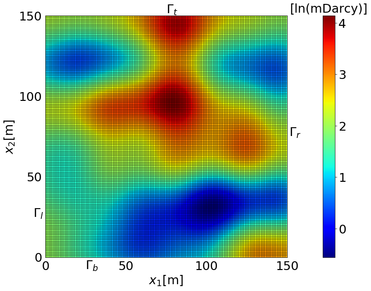
Figure 2: A representative realization of log permeability field $Y=\ln k$ on the $128\times 128$ grid, which is used in high-fidelity simulations. Permeability $k$ is expressed in mDarcy.

All the model parameters, except for the intrinsic permeability $k(\mathbf{x})$, are assumed to be constant and known with certainty. The uncertain permeability $k(\mathbf{x})$ is modeled as a second-order stationary random field, such that $Y(\mathbf{x})=\ln k$ is multivariate Gaussian with mean $\langle Y\rangle=0$, variance $\sigma^{2}_{Y}=2.0$, and an exponential two-point covariance $C(\mathbf{x},\mathbf{y})=\sigma^{2}_{Y}\exp(-|\mathbf{x}-\mathbf{y}|/\lambda_{Y})$ with the correlation length $\lambda_{Y}=19$ m. We use a truncated Karhunen-Loéve expansion with $p=31$ terms to represent $Y(\mathbf{x})$ (Taverniers et al., 2020). A representative realization of the resulting permeability field is shown in Fig. 2 for the $128\times 128$ mesh.

Equations (3)–(4) are approximated using a finite volume scheme in space and implicit Euler scheme in time, yielding a highly nonlinear algebraic system (Aziz, 1979). The latter is solved, at each time step, through Newton-Raphson (NR) iterations with the modified Appleyard update dampening (Appleyard et al., 1981) that improves the convergence of NR iterations by capping the maximum saturation update to a specified limit. For the $\nu$th iteration and the $i$th cell of volume $V_{i}$, the convergence criteria are

$$\max_{i}\left|\Delta t\left(\frac{r_{\ell,i}}{\phi V_{i}}\right)\right|<\epsilon_{1},\quad\max_{i}|P_{i}^{(\nu+1)}-P_{i}^{(\nu)}|<\epsilon_{2},\quad\max_{i}|S_{\ell,i}^{(\nu+1)}-S_{\ell,i}^{(\nu)}|<\epsilon_{3}$$ (5)

where $r_{\ell,i}$ is the residual of the mass balance of phase $\ell$, $\Delta t$ is the time step, the relative residual norm $\epsilon_{1}=10^{-6}$, the maximum pressure update $\epsilon_{2}=10^{-3}$, and the maximum saturation update $\epsilon_{3}=10^{-2}$.

3.1 Upscaling of Permeability

Multi-fidelity data are generated by solving (3)–(4) on progressively coarsened grids: the $128\times 122$ and $64\times 64$ grids are used for HFS and LFS, respectively. This grid coarsening must be accomplished by upscaling (coarsening) of the realizations of the random permeability $\hat{k}$ which are initially generated at the finest scale (Fig. 2). Among alternative upscaling strategies (Paleologos et al., 1996; Tartakovsky and Neuman, 1998; Boso and Tartakovsky, 2018), we select the one proposed by Durlofsky (2005) because of its computational simplicity. It turns a scalar permeability field defined on the fine $(128\times 128)$ mesh into its upscaled tensorial (anisotropic) counterpart whose off-diagonal components are 0 and the diagonal components are computed as the distance-weighted arithmetic mean perpendicular to the direction of flow and the distance-weighted harmonic mean in the direction of flow.

3.2 Data Acquisition

Multi-fidelity training data come in the form of $N_{\text{ts}}=16$ temporal snapshots of the saturation $S_{1}(\mathbf{x},t)$ computed by solving (3)–(4) on the $N_{\text{el}}\times N_{\text{el}}$ grids with $N_{\text{el}}=128\equiv N_{\text{el}}^{\text{HFS}}$ and $64\equiv N_{\text{el}}^{\text{LFS}}$. Fig. 3 shows examples of such images, corresponding to the permeability field in Fig. 2. The permeability fields on the finest mesh, $[1\times N_{\text{HFS}}\times N_{\text{HFS}}]$, are used as the input $\bm{\theta}$ for all CNNs. The size of of the CNN, $[N_{\text{ts}}\times N_{\text{el}}\times N_{\text{el}}]$, depends on the size of the training data.

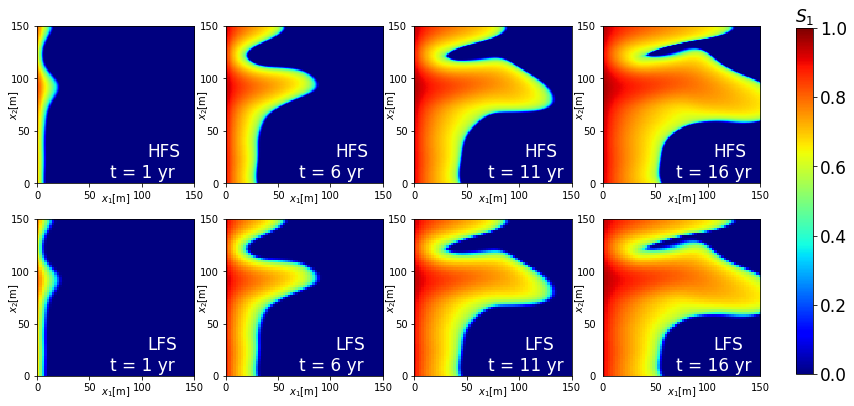
Figure 3: Temporal snapshots of saturation $S_{1}(\mathbf{x},t)$ computed with HFS (top-row) and LFS (bottom-row) for the permeability field $k(\mathbf{x})$ in Fig. 2.

The numerical solutions of (3)–(4) are obtained using a Matlab-based multi-phase flow simulator on a computer with an Intel Core i7-4790 3.6GHz processor and 64GB of RAM. The computation time for each HFS data point is 219.13 sec and 37.13 sec for each LFS data point. The time needed to generate a data set is henceforth referred as “data-generation budget”.

3.3 CNN Training

Table 1 describes the CNN architecture used in this implementation our general approach (see Fig 1). The training is done with PyTorch, on the Stanford Mazama high-performance computing cluster. The allocated computing resources include Intel Xenon Gold 6126 CPU (2.6 GHz), 60GB RAM, and Nvidia V100 GPU with 16GB vRAM. (Although available, multi-cores were not used for this work.)

Table 1: Model block description and the input and output dimensions of each model block. In our numerical experiments, the number of time steps is $N_{\text{ts}}=16$; the number of elements in fine and coarse meshes is $N_{\text{el}}^{\text{HFS}}=128$ and $N_{\text{el}}^{\text{LFS}}=64$, respectively; the number of elements in the output of the dense block is $N_{\text{dense}}=32$; and the number of channels in each of the seven layers of the CNN is $n_{1}=64$, $n_{2}=344$, $n_{3}=172$, $n_{4}=652$, $n_{5}=326$, $n_{6}=606$, and $n_{7}=303$.

Layer	Input	Output
Input: Permeability field $k$	$1\times N_{\text{HFS}}\times N_{\text{HFS}}$
Convolution 1	$n_{1}\times N_{\text{el}}^{\text{HFS}}\times N_{\text{el}}^{\text{HFS}}$	$n_{2}\times N_{\text{el}}^{\text{LFS}}\times N_{\text{el}}^{\text{LFS}}$
Dense Block (Encoding)	$n_{2}\times N_{\text{el}}^{\text{LFS}}\times N_{\text{el}}^{\text{LFS}}$	$n_{3}\times N_{\text{el}}^{\text{LFS}}\times N_{\text{el}}^{\text{LFS}}$
Convolution 2	$n_{3}\times N_{\text{LFS}}\times N_{\text{el}}^{\text{LFS}}$	$n_{4}\times N_{\text{el}}^{\text{dense}}\times N_{\text{dense}}$
Dense Block	$n_{4}\times N_{\text{dense}}\times N_{\text{dense}}$	$n_{5}\times N_{\text{dense}}\times N_{\text{dense}}$
Convolution Transpose 1	$n_{5}\times N_{\text{dense}}\times N_{\text{dense}}$	$n_{6}\times N_{\text{el}}^{\text{LFS}}\times N_{\text{el}}^{\text{LFS}}$
Dense Block (Decoding)	$n_{6}\times N_{\text{el}}^{\text{LFS}}\times N_{\text{el}}^{\text{LFS}}$	$n_{7}\times N_{\text{el}}^{\text{LFS}}\times N_{\text{el}}^{\text{LFS}}$
Convolution Transpose 2	$n_{7}\times N_{\text{el}}^{\text{LFS}}\times N_{\text{el}}^{\text{LFS}}$	$N_{\text{ts}}\times N_{\text{el}}^{\text{HFS}}\times N_{\text{el}}^{\text{HFS}}$
Output: Saturation map $\hat{S}$	$N_{\text{ts}}\times N_{\text{el}}^{\text{HFS}}\times N_{\text{el}}^{\text{HFS}}$

The key hyper-parameters affecting the CNN performance are the learning rate (LR), the weight decay (WD), the factor (F), and the minimum learning rate (mLR). The LR and WD are parameters of the Adam optimizer (Kingma and Ba, 2014), and the F and mLR are parameters of the ReduceLROnPlateau scheduler. The CNN training involves many more hyper-parameters, but we use their default values in PyTorch. Further information on the hyper-parameters, schedulers, and optimizers can be found in the PyTorch documentation (Paszke et al., 2019).

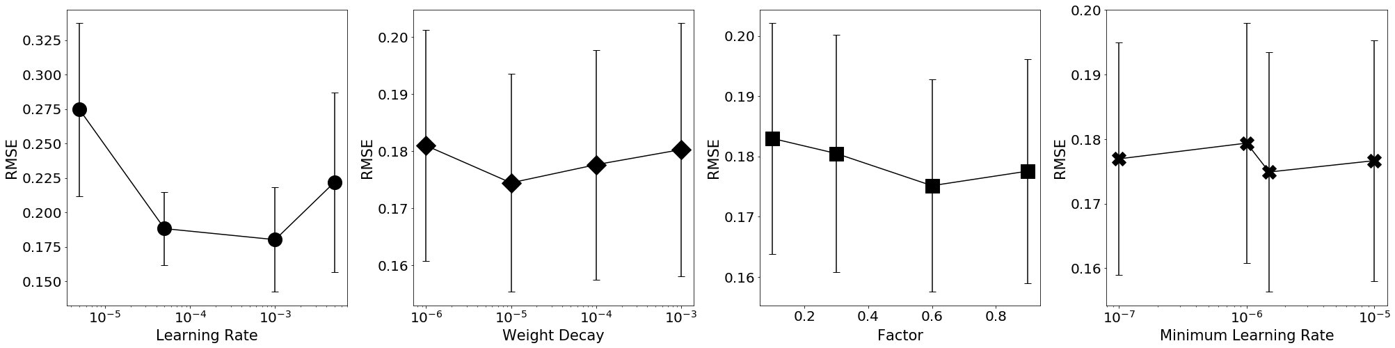
Figure 4: Hyper-parameter performance in the neighborhood of optimum hyper parameter set in terms of the root mean square error (RMSE) for the test data. Unless labeled as the $x$-axis variable, all plot correspond to $\text{LR}=5\cdot 10^{-5}$, $\text{WD}=1\cdot 10^{-5}$, $\text{F}=0.6$, and $\text{mLR}=5\cdot 10^{-6}$. Each data point represents the mean and standard deviation of 10 training sessions.

Table 2: Learning rates and epochs used at each Phase.

	Learning rate	Epochs
Phase 1	$5\cdot 10^{-4}$	170
Phase 2	$5\cdot 10^{5}$	150
Phase 3	$10^{-5}$	100

The hyper-parameters used by Mo et al. (2019b) in a similar CNN architecture serve as an initial guess for the hyper-parameter optimization. The latter required 100 HFS, with each training pass taking about 0.65 hours to complete, when 200 epochs were used. It took 7.2 training-hours to find optimal hyper-parameters (12 training passes), and a considerably smaller wall-clock time because this task was parallelized across several GPU nodes. We selected the hyper-parameter values yielding the smallest root mean square error (RMSE) on the HFS test data (Fig. 4). These values are used as a starting point in the hyper-parameter optimization for multi-fidelity transfer learning. Then, the LR and epochs at each Phase (Section 2.2) are modified to minimize the RMSE on the corresponding test data. The resulting hyper-parameter values are shown in Table 2.

4 Results

Once trained (in this example, on 573 LFS and 100 HFS, which took 12 hours to generate), the CNN surrogate provides an accurate approximation of the PDE solution on the fine mesh (Fig. 5), even for such highly nonlinear problems as (3) that exhibit sharp dynamic fronts. A forward pass of the CNN surrogate is on the order of a second, whereas a fine-mesh PDE solution takes nearly 220 seconds. This two-orders of magnitude speed up makes CNN surrogates an invaluable tool for UQ (Section 4.2).

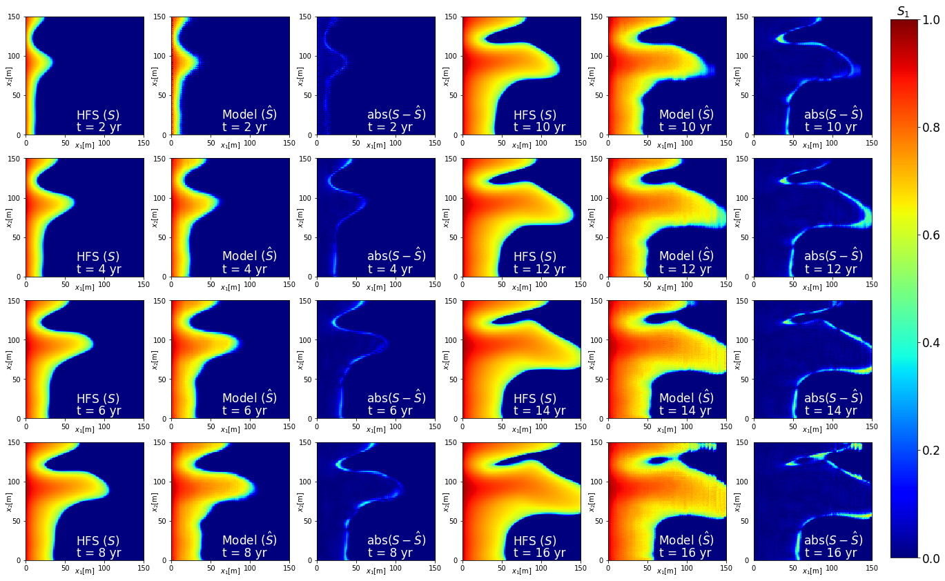
Figure 5: Temporal snapshots of the saturation maps $S_{1}(\mathbf{x},t)$ for the permeability field $k(\mathbf{x})$ in Fig. 2. These are generated with either HFS of the PDE model (3) and (4) (labeled as $S$ in the first and fourth columns) or the CNN surrogate (labeled as $\hat{S}$) in the second and fifth columns). The third and sixth columns display the absolute difference between the two predictions, $|S-\hat{S}|$.

4.1 Model Performance

We compare the relative performance of the CNN trained on multi-fidelity data and the CNNs trained on either HFS data or LFS data, in terms of both accuracy (RMSE on test data) and computational cost. We also investigate the effect of varying the amount of HFS and LFS data for a given computational budget of 12 hours.

To train the high-resolution ($128\times 128$ output) CNN solely on the LFS ($64\times 64$) data, the latter have to be downscaled to match the dimensions. We do so by taking the Kronecker product of a $64\times 64$ LFS image and a $2\times 2$ matrix of 1s. The transformed LFS data have the desired dimensions, while containing the same information as the original image. The test data are composed of HFS images (PDE solves on fine mesh) that were not used for CNN training. Figure 6 exhibits the RMSEs on test data of the CNNs trained on high-, low-, and multi-fidelity data as function of the computational budget; each point in these graphs represents an average over 10 repetitions of training and is accompanied by error bars (the standard deviation).

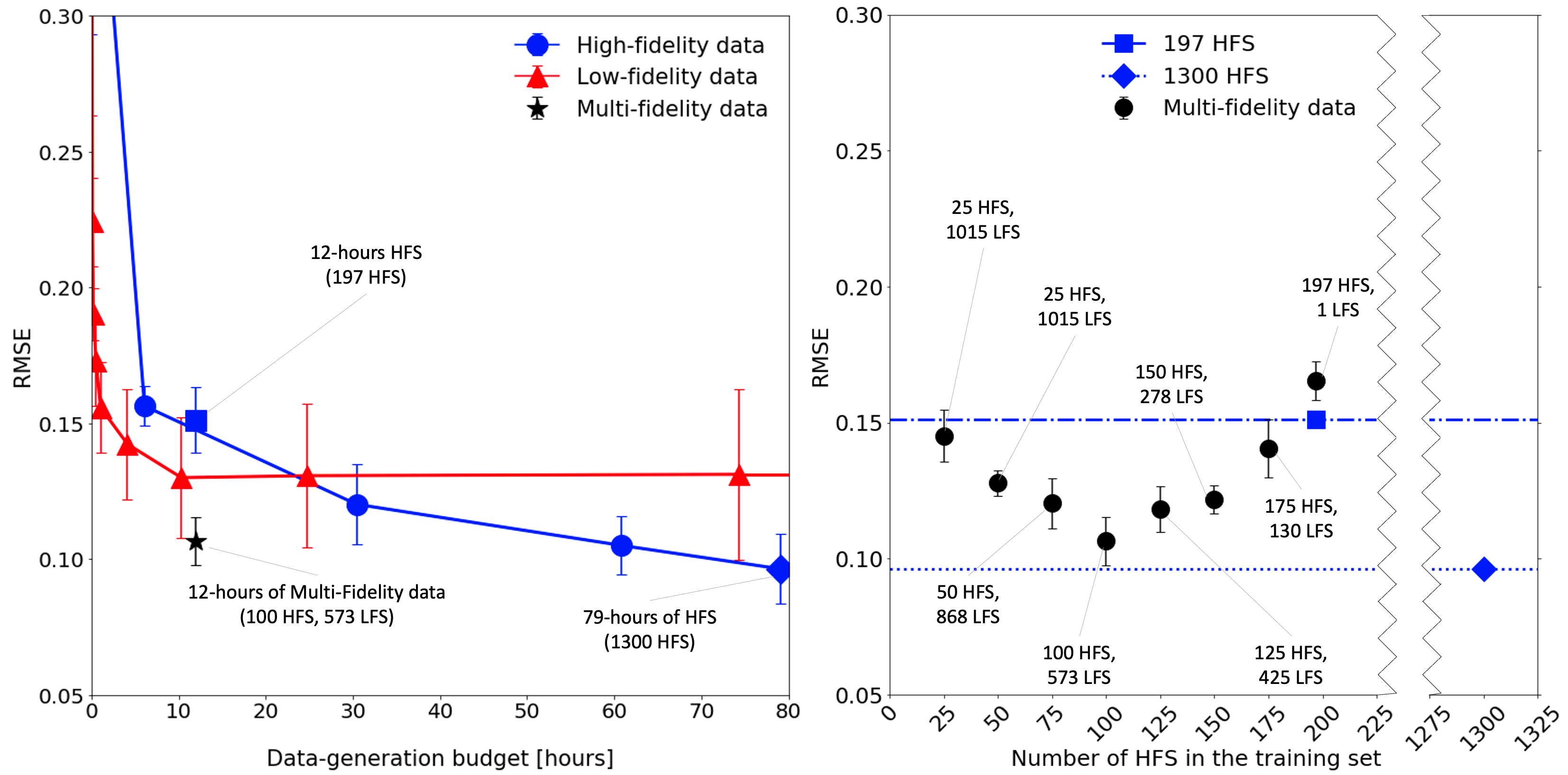
Figure 6: RMSE on test data for the alternative CNN training strategies. It is plotted as function of the budget allocated for data generation (left) and the number of PDE solves on the fine mesh used to generate HFS data (right). Each RMSE point in these graphs represents an average over 10 iterations of training and is accompanied by error bars (the standard deviation). The left plate provides RMSE for the CNNs trained on high-fidelity (blue circles), low-fidelity (red triangles), or multi-fidelity (black star) data. The latter corresponds to the CNN trained on an optimal (the lowest RMSE) mix of high- and low-fidelity data for a set budget of 12 hours; it is contrasted with the RMSE of the CNN trained on the HFS data generated within the same budget (blue square). The black circles in the right plate represent RMSE of the CNN trained on the multi-fidelity data sets, in which the number of HFS varies while the data-generation budget is fixed at 12 hours. Also shown there are RMSEs of the CNNs trained on 12 hours (dot-dashed line) and 79 hours (dotted line) of HFS.

The left plate of Fig. 6 reveals that, if the data-generation budget does not exceed 20 hours, the CNN trained on the LFS data outperforms its HFS-trained counterpart in terms of RMSE. That is because such budgets do not allow for generation of sufficient amounts of HFS data. As the budget increases, the error of the LFS data precludes RMSE of the CNN trained on such data from dropping below 0.125 while RMSE of the HFS-trained CNN continues to decrease. This finding is reminiscent of the cost-constrained selection between high- and low-fidelity models in the context of ensemble-based simulations (Yang et al., 2020; Sinsbeck and Tartakovsky, 2015). This figure also demonstrates that, for a relatively small budget of 12 hours, the use of multi-fidelity data yields the CNN whose RMSE is appreciably smaller that those of the CNNs trained on either HFS data or LFS data.

An optimal mix of the HFS and LFS data is investigated in the right plate of Fig. 6. The multi-fidelity training was conducted 5 times for each HFS/LFS ratio, with random selection of LFS/HFS from a larger pool data. At the optimal mix of 573 LFS and 100 HFS, two of the five experiments, the CNN trained on 12 hours of these multi-fidelity data has lower RMSE than the mean RMSE of the CNN trained on 79 hours of the HFS data. This LFS/HFS ratio lies near the range, $1.5-5.5$, suggested for multilevel Monte Carlo (Taverniers et al., 2020). For the data-generation budget of 12 hours, a mix dominated by the LFS data results in a CNN whose RMSE on test data exceeds 1.0, which indicates that the network’s last Convolution Transpose 2 layer is not meaningfully trained.

4.2 CNN Surrogates for Uncertainty Quantification

Finally, we investigate the utility of our CNN surrogates for uncertainty quantification. A quantity of interest is the breakthrough time, $T_{\text{break}}$, at the $x_{1}=100$ m plane (Fig. 2), with the term “breakthrough” defined as the saturation of the invading phase ($S_{1}$) exceeding 0.15. Given uncertainty in intrinsic permeability $k(\mathbf{x})$, a solution of (3) and, hence, predictions of $T_{\text{break}}$ are given in terms of their cumulative distribution functions (CDFs) or probability density functions (PDFs).

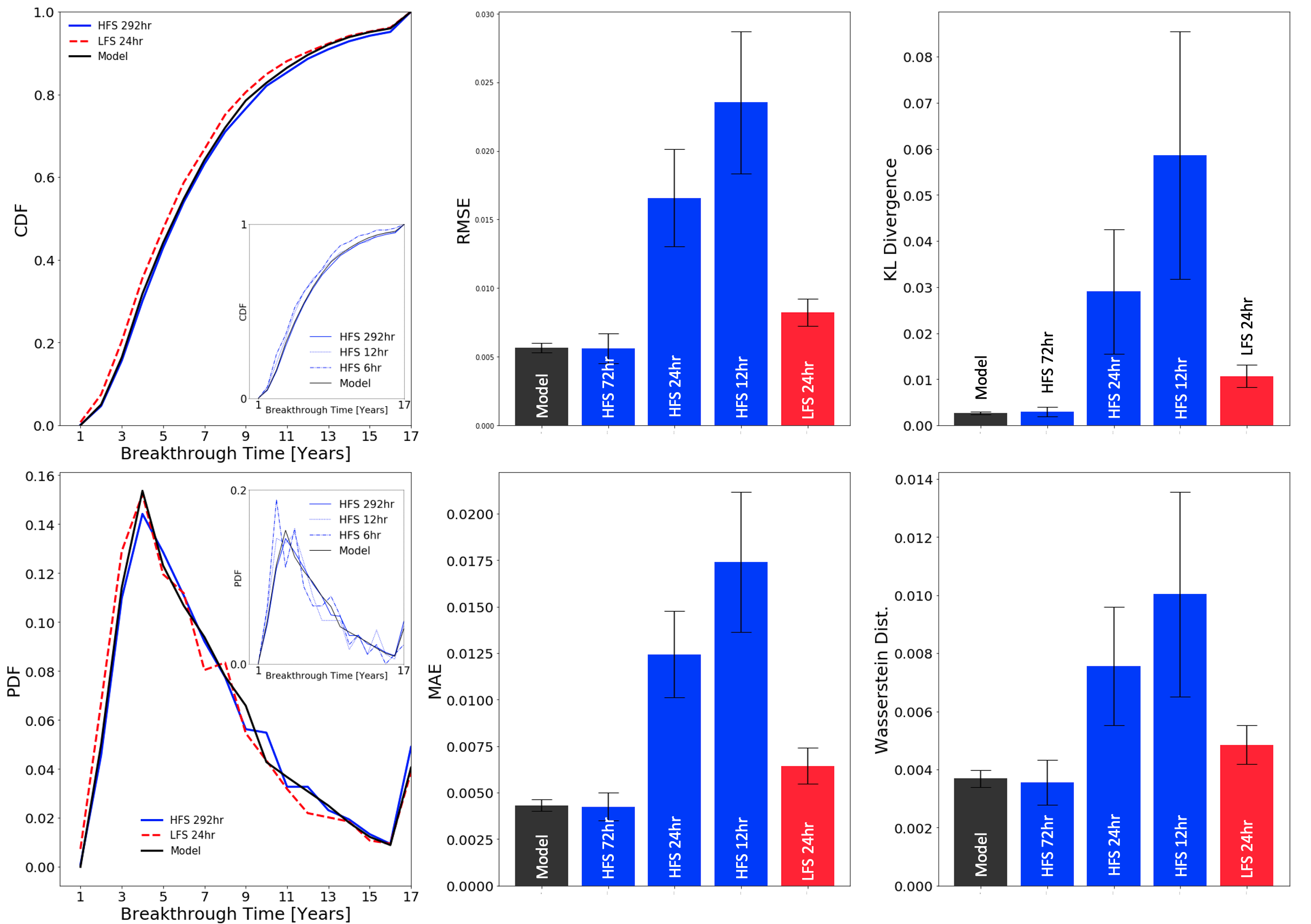
Figure 7: Left: The converged CDF (top) and PDF (bottom) of breakthrough time is calculated using MC simulations of HFS, LFS, and the CNN surrogate model. The CDF and PDF calculated from varying amounts of HFS are displayed on the subplots. Bar plots: RMSE (Middle-top), MAE (Middle-bottom), KL Divergence (Right-top), and Wasserstein distance (Right-bottom) from PDF calculated using CNN model, HFS, and LFS.

Figure 7 exhibits the CDF and PDF of $T_{\text{break}}$ alternatively computed with HFS and LFS Monte Carlo and with the CNN trained on the multi-fidelity data. The distributions obtained via Monte Carlo consisting of 282 hours of HFS are treated as ground truth. The distributions obtained from 24 hours of LFS involve a sufficient number of samples for the error to be attributable solely to the low resolution, i.e., to the disretization errors in solving PDEs. The numbers of HFS samples generated during either 6 or 12 hours of simulations are insufficient for Monte Carlo to converge, leading to the appreciable errors in estimation of PDF and CDF of $T_{\text{break}}$. The CNN trained on multi-fidelity data yields accurate estimates of these quantities, while requiring only 12 hours of data generation.

In addition to visual comparison, the alternative strategies for estimation of the distributions of $T_{\text{break}}$ are compared in terms of RMSE, mean absolute error (MAE), the Kullback-Leibler (KL) divergence, and the Wasserstein distance. The UQ task was repeated 50 times, with Fig. 7 displaying the mean and standard deviation of these measures of discrepancy. We found 3200 forward passes of the CNN to be sufficient for the CDF/PDF estimates to converge; this UQ task took about 10 minutes, whereas an equivalent HFS Monte Carlo takes 194 hours. By every discrepancy measure, the CNN estimates outperform the converged LFS Monte Carlo and are at least as accurate as the HFS Monte Carlo using 72 hours of data. Likewise, the CNN estimates are vastly more accurate than the HFS Monte Carlo of a similar data-generation budget.

5 Conclusions

We proposed a transfer learning-based approach to train a CNN on multi-fidelity (e.g., multi-resolution) data. High- and low-fidelity images were generated by solving a PDE on fine and coarse meshes, respectively. The performance of our algorithm was tested on a system of nonlinear parabolic PDEs governing multi-phase flow in a heterogeneous porous medium with uncertain (random) permeability. A quantity of interest (QoI) in this example is PDF or CDF of the breakthrough time of an invading fluid. Our analysis leads to the following major conclusions.

1. CNN surrogates trained on multi-fidelity data provide an accurate approximation of the PDE solution on the fine mesh, even for highly nonlinear problems that exhibit sharp dynamic fronts. A forward pass of the CNN surrogate is two orders of magnitude faster than a PDE solution on the fine-mesh. This speed-up makes CNN surrogates an invaluable tool for ensemble-based computation of the PDF/CDF of a QoI.

2. CNN training on multi-fidelity data reduces the data-generation budget 7-fold relative to to CNN training on HFS data alone. If the budget is relatively small, the CNN trained on the LFS data is more accurate than its HFS-trained counterpart. As the budget increases, the opposite is true. This finding is reminiscent of the cost-constrained selection between high- and low-fidelity models in the context of ensemble-based simulations.

3. For a small data-generation budget (12 hours, in our example), the CNN trained on multi-fidelity data exhibits an appreciably smaller RMSE on test data than the CNNs trained on either HFS or LFS data. Performance of the multi-fidelity CNN depends on the ratio between HFS and LFS in the training set. Theoretical studies from multilevel Monte Carlo can be used to guide the selection of an optimal mix of low- and high-fidelity data.

4. The CNN trained on multi-fidelity data is largely insensitive to the discretization error of LFS. CNN-derived estimates of the PDF and CDF of the QoI are close to those of converged high-fidelity Monte Carlo; but the former are three orders of magnitude faster to obtain than the latter.

References

- Appleyard et al. (1981) Appleyard, J.R., Cheshire, I.M., and Pollard, R.K., \titlecapSpecial techniques for fully implicit simulators, Proceedings of the European Symposium on Enhanced Oil Recovery, Bournemouth, UK, pp. 395–408, 1981.
- Aziz (1979) Aziz, K., \titlecapPetroleum reservoir simulation, Vol. 476, Applied Science Publishers, New York, 1979.
- Boso and Tartakovsky (2018) Boso, F. and Tartakovsky, D.M., \titlecapInformation-theoretic approach to bidirectional scaling, Water Resour. Res., vol. 54, no. 7, pp. 4916–4928, 2018.
- Breiman (2001) Breiman, L., \titlecapRandom forests, Mach. Learn., vol. 45, no. 1, pp. 5–32, 2001.
- Corey (1954) Corey, A.T., \titlecapThe interrelation between gas and oil relative permeabilities, Producers Month., vol. 19, no. 1, pp. 38–41, 1954.
- Couckuyt et al. (2014) Couckuyt, I., Dhaene, T., and Demeester, P., \titlecapSooDACE Toolbox: A Flexible Object-Oriented Kriging Implementation, J. Mach. Learn. Res., vol. 15, pp. 3183–3186, 2014.
- Donahue et al. (2014) Donahue, J., Jia, Y., Vinyals, O., Hoffman, J., Zhang, N., Tzeng, E., and Darrell, T., \titlecapDecaf: A deep convolutional activation feature for generic visual recognition, International Conference on Machine Learning, PMLR, pp. 647–655, 2014.
- Durlofsky (2005) Durlofsky, L.J., \titlecapUpscaling and gridding of fine scale geological models for flow simulation, 8th International Forum on Reservoir Simulation, Vol. 2024, Iles Borromees, Stresa, Italy, pp. 1–59, 2005.
- Friedman et al. (2001) Friedman, J., Hastie, T., and Tibshirani, R., \titlecapThe elements of statistical learning, Vol. 1, Springer, New York, 2001.
- Fuks and Tchelepi (2020) Fuks, O. and Tchelepi, H., \titlecapLimitations of physics informed machine learning for nonlinear two-phase transport in porous media, J. Mach. Learn. Model. Comput., vol. 1, no. 1, pp. 19–37, 2020.
- Giles (2008) Giles, M.B., \titlecapMultilevel Monte Carlo path simulation, Oper. Res., vol. 56, no. 3, pp. 607–617, 2008.
- Haghighat et al. (2021) Haghighat, E., Raissi, M., Moure, A., Gomez, H., and Juanes, R., \titlecapA physics-informed deep learning framework for inversion and surrogate modeling in solid mechanics, Comput. Meth. Appl. Mech. Engrg., vol. 379, p. 113741, 2021.
- Heinrich (1998) Heinrich, S., \titlecapMonte Carlo complexity of global solution of integral equations, J. Complexity, vol. 14, no. 2, pp. 151–175, 1998.
- Heinrich (2001) Heinrich, S., \titlecapMultilevel Monte Carlo methods, International Conference on Large-Scale Scientific Computing, Springer, pp. 58–67, 2001.
- Hwang and Martins (2018) Hwang, J.T. and Martins, J.R.R.A., \titlecapA fast-prediction surrogate model for large datasets, Aerospace Sci. Tech., vol. 75, pp. 74–87, 2018.
- Jiang and Learned-Miller (2017) Jiang, H. and Learned-Miller, E., \titlecapFace detection with the faster R-CNN, 2017 12th IEEE International Conference on Automatic Face & Gesture Recognition (FG 2017), IEEE, pp. 650–657, 2017.
- Karpathy and Fei-Fei (2015) Karpathy, A. and Fei-Fei, L., \titlecapDeep visual-semantic alignments for generating image descriptions, Proceedings of the IEEE Conference on Computer Vision and Pattern Recognition, pp. 3128–3137, 2015.
- Kingma and Ba (2014) Kingma, D.P. and Ba, J., \titlecapAdam: A method for stochastic optimization, arXiv:1412.6980, 2014.
- Lagaris et al. (1998) Lagaris, I.E., Likas, A., and Fotiadis, D.I., \titlecapArtificial neural networks for solving ordinary and partial differential equations, IEEE Trans. Neural Networks, vol. 9, no. 5, pp. 987–1000, 1998.
- Lee and Kang (1990) Lee, H. and Kang, I.S., \titlecapNeural algorithm for solving differential equations, J. Comput. Phys., vol. 91, no. 1, pp. 110–131, 1990.
- Mo et al. (2019a) Mo, S., Zabaras, N., Shi, X., and Wu, J., \titlecapDeep autoregressive neural networks for high-dimensional inverse problems in groundwater contaminant source identification, Water Resour. Res., vol. 55, no. 5, pp. 3856–3881, 2019a.
- Mo et al. (2019b) Mo, S., Zhu, Y., Zabaras, N., Shi, X., and Wu, J., \titlecapDeep convolutional encoder-decoder networks for uncertainty quantification of dynamic multiphase flow in heterogeneous media, Water Resour. Res., vol. 55, no. 1, pp. 703–728, 2019b.
- Montgomery and Evans (2018) Montgomery, D.C. and Evans, D.M., \titlecapSecond-order response surface designs in computer simulation, Aerospace Sci. Tech., vol. 75, pp. 74–87, 2018.
- Müller et al. (2013) Müller, F., Jenny, P., and Meyer, D.W., \titlecapMultilevel Monte Carlo for two phase flow and Buckley-Leverett transport in random heterogeneous porous media, J. Comput. Phys., vol. 250, pp. 685–702, 2013.
- Paleologos et al. (1996) Paleologos, E.K., Neuman, S., and Tartakovsky, D.M., \titlecapEffective hydraulic conductivity of bounded, strongly heterogeneous porous media, Water Resour. Res., vol. 32, no. 5, pp. 1333–1341, 1996.
- Paszke et al. (2019) Paszke, A., Gross, S., Massa, F., Lerer, A., Bradbury, J., Chanan, G., Killeen, T., Lin, Z., Gimelshein, N., Antiga, L., Desmaison, A., Kopf, A., Yang, E., DeVito, Z., Raison, M., Tejani, A., Chilamkurthy, S., Steiner, B., Fang, L., Bai, J., and Chintala, S., 2019. Pytorch: An imperative style, high-performance deep learning library, Advances in Neural Information Processing Systems 32. H. Wallach, H. Larochelle, A. Beygelzimer, F. d'Alché-Buc, E. Fox, and R. Garnett, Eds. Curran Associates, Inc., pp. 8024–8035.
- Peherstorfer (2019) Peherstorfer, B., \titlecapMultifidelity Monte Carlo Estimation with Adaptive Low-Fidelity Models, SIAM/ASA J. Uncert. Quant., vol. 7, no. 2, p. 579–603, 2019.
- Raissi et al. (2019) Raissi, M., Perdikaris, P., and Karniadakis, G.E., \titlecapPhysics-informed neural networks: A deep learning framework for solving forward and inverse problems involving nonlinear partial differential equations, J. Comput. Phys., vol. 378, pp. 686–707, 2019.
- Sinsbeck and Tartakovsky (2015) Sinsbeck, M. and Tartakovsky, D.M., \titlecapImpact of data assimilation on cost-accuracy tradeoff in multifidelity models, SIAM/ASA J. Uncert. Quant., vol. 3, no. 1, pp. 954–968, 2015.
- Tang et al. (2020) Tang, M., Liu, Y., and Durlofsky, L.J., \titlecapA deep-learning-based surrogate model for data assimilation in dynamic subsurface flow problems, J. Comput. Phys., p. 109456, 2020.
- Tartakovsky and Neuman (1998) Tartakovsky, D.M. and Neuman, S.P., \titlecapTransient effective hydraulic conductivities under slowly and rapidly varying mean gradients in bounded three-dimensional random media, Water Resour. Res., vol. 34, no. 1, pp. 21–32, 1998.
- Taverniers et al. (2020) Taverniers, S., Bosma, S.B., and Tartakovsky, D.M., \titlecapAccelerated multilevel Monte Carlo with kernel-based smoothing and Latinized stratification, Water Resour. Res., vol. 56, no. 9, p. e2019WR026984, 2020.
- Tripathy and Bilionis (2018) Tripathy, R.K. and Bilionis, I., \titlecapDeep UQ: Learning deep neural network surrogate models for high dimensional uncertainty quantification, J. Comput. Phys., vol. 375, pp. 565–588, 2018.
- Xiu (2010) Xiu, D., \titlecapNumerical Methods for Stochastic Computations: A spectral Methd Approach, Princeton University Press, Princeton, NJ, 2010.
- Yang et al. (2020) Yang, L., Wang, P., and Tartakovsky, D.M., \titlecapResource-constrained model selection for uncertainty propagation and data assimilation, SIAM/ASA J. Uncert. Quant., vol. 8, no. 3, pp. 1118–1138, 2020.
- Zhou and Tartakovsky (2021) Zhou, Z. and Tartakovsky, D.M., \titlecapMarkov chain Monte Carlo with neural network surrogates: Application to contaminant source identification, Stoch. Environ. Res. Risk Assess., vol. 35, no. 3, pp. 639–651, 2021.
- Zhu et al. (2019) Zhu, Y., Zabaras, N., Koutsourelakis, P.S., and Perdikaris, P., \titlecapPhysics-constrained deep learning for high-dimensional surrogate modeling and uncertainty quantification without labeled data, J. Comput. Phys., vol. 394, pp. 56–81, 2019.