Multivariate tempered stable additive subordination for financial models

Abstract

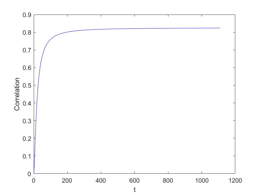
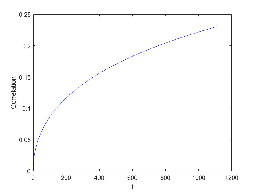
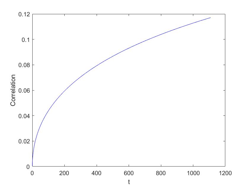
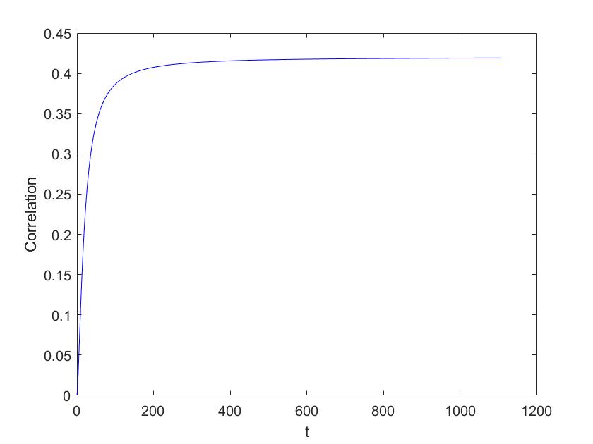
We study a class of multivariate tempered stable distributions and introduce the associated class of tempered stable Sato subordinators. These Sato subordinators are used to build additive inhomogeneous processes by subordination of a multiparameter Brownian motion. The resulting process is additive and time inhomogeneous. Furthermore, these processes are associated with the distribution at unit time of a class of Lévy process with good fit properties on financial data. The main feature of the Sato subordinated Brownian motion is that it has time dependent correlation, whereas the Lévy counterpart does not. We choose a specification with normal inverse Gaussian distribution at unit time and provide a numerical illustration of the correlation dynamics.

Mathematics Subject Classification (2000): 60G51, 60E07.

Keywords: Tempered stable distributions, Sato processes, multivariate additive subordination, multivariate asset modelling.

Introduction

Additive processes with independent but inhomogeneous increments have been proposed to model asset returns. Carr et al., (2007) showed that these processes can synthesize the surface of option prices and Eberlein and Madan, (2009) empirically analysed the use of Sato processes in the valuation of equity structured products.

A class of additive processes with inhomogeneous increments used in finance are Sato processes. Sato, (1999) showed that given a self decomposable law $\mu$ an additive process $Y(t)$ always exists such that $Y(1)\sim\mu$ and the time $t$ distribution is the law of $t^{q}Y(1)$. Eberlein and Madan, (2009) termed this additive process the Sato process. Sato processes exhibit a moment term structure in line with the one observed in financial markets, see Boen and Guillaume, (2019).

A possible approach to include time inhomogeneity in financial models is to use additive subordination; see Mendoza-Arriaga and Linetsky, (2016), Li et al., (2016) and Kokholm and Nicolato, (2010). In this case inhomogeneity comes from the subordinator.

The success of subordination in finance is due to many reasons. Price processes under no arbitrage are semimartingales and these can be represented as time-changed Brownian motions. Furthermore, time change models economic time: the more intense the market activity, the faster economic time runs relative to calendar time. When the change of time is a subordinator, the resulting process belongs to the (pure jump) Lévy class, a class of analytically tractable processes. In the one-dimensional case, the most famous subordinated Brownian motions such as the variance gamma and the normal inverse Gaussian processes have unit time self-decomposable distributions. Therefore it is possible to define the corresponding Sato processes. Unfortunately, in multivariate subordination this is no longer true.

In Takano, (1989), the author gave conditions for a multivariate subordinated Brownian motion to have self-decomposable unit time distribution. The author considered the subcase of a one-dimensional generalized gamma subordinator. Even in this case he found that if the Brownian motion has non-zero drift the subordinated process distribution at unit time is not self-decomposable. As a consequence, multivariate subordinated Brownian motions are not good candidates to construct multivariate Sato processes. However, it is possible to consider multivariate self-decomposable distributions to define multivariate Sato subordinators. Sato subordinators associated to self-decomposable distributions are easy to construct, introduce time inhomogeneity and perform well on financial data (Sun et al., (2017)). Therefore, it is possible to use additive subordination of multivariate Brownian motions to obtain additive processes with inhomogeneous increments to model asset returns.

In this paper we introduce and study a self-decomposable class of multivariate exponential tempered distributions and the associated multivariate Sato subordinators. This class is defined as a particular case of the tempered distributions in Rosiński, (2007) and it is a generalization of the multivariate gamma distribution in Pérez-Abreu and Stelzer, (2014). Exponential tempered stable distributions are a multivariate version of the self-decomposable distributions most used in finance, such as the famous CGMY (Carr et al., (2002)), the variance gamma (Madan and Seneta, (1990)), the bilateral gamma (Küchler and Tappe, (2008)), the gamma and the inverse Gaussian distributions. We study some properties of multivariate exponential tempered stable distributions, for example Proposition 2.2 provides the existence conditions for their moments and Proposition 3.1 provides conditions for them to be the distributions at unit time of Sato subordinators. We then characterize multivariate Sato subordinators by providing their time t Lévy measure in Theorem 3.1 and we focus on a specific dependence structure widely used in finance to include correlations in multivariate models.

Finally, we build a multivariate additive process using additive multivariate subordination of a Brownian motion. The construction is designed to have a multivariate process with the same unit time distribution as the factor-based $\rho\alpha$-model in Luciano and Semeraro, 2010b . This process has one-dimensional marginal processes that are themselves subordinated Brownian motions. Therefore, choosing the subordinator properly, the one-dimensional processes are self-decomposable. Making use of this and building on the construction proposed in Guillaume, (2012), Marena et al., (2018) introduced a multivariate process with the same unit time distribution of the $\rho\alpha$-models and one-dimensional marginal Sato processes. Although this process has time inhomogeneous increments, its correlation is constant over time, as in the original Lévy motion. For simplicity, correlations are assumed to be constant in many financial models, however this is not a realistic assumption, see e.g. Tóth and Kertész, (2006), Teng et al., (2016) and Lundin et al., (1998).

The main contribution of Sato subordination is to provide time varying correlations, while maintaining the features of the $\rho\alpha$-models dependence structure and remaining parsimonious in the number of parameters. Last but not least, as with for the Lévy and the marginal Sato models, Theorem 4.1 and its Corollary 5.2 provide the characteristic function in closed form. Although the empirical investigation of this model is beyond the scope of this work, we conclude with a numerical illustration of the correlation dynamics.

The paper is organized as follows. Section 1 introduces tempered stable distributions. Exponential tempered stable distributions are studied in Section 2, while Section 3 defines the corresponding Sato subordinators. Section 4 discusses multivariate Sato subordination of a multiparameter Brownain motion. The specification of an asset return model is developed in Section 5 with numerical illustration. Section 6 concludes.

1 Tempered stable distributions

This section introduces multivariate stable and tempered stable distributions.

Let $\mu$ be an infinitely divisible distribution on $\mathbb{R}^{d}$ without Gaussian component and $\nu$ its Lévy measure. The following proposition provides the polar decomposition of the Lévy measure $\nu$ (see e.g. Maejima et al., (2009) and Rosinski, (1990)).

Proposition 1.1.

Let $\nu$ be a Lévy measure. Then it exists a measure $\lambda$ on $S^{d-1}$ with $0<\lambda(S^{d-1})\leq\infty$ and a family $\{\nu_{\boldsymbol{w}}:\boldsymbol{w}\in S^{d-1}\}$ of measures on $(0,\infty)$, $0<\nu_{\boldsymbol{w}}(\mathbb{R}_{+})\leq\infty$, such that $\nu_{\boldsymbol{w}}(E)$ is measurable in $\boldsymbol{w}$ for any $E\in\mathcal{B}((0,\infty))$ and it is $\sigma$-finite for any $\boldsymbol{w}\in S^{d-1}$,

$$\int_{0}^{1}r^{2}\nu_{\boldsymbol{w}}(dr)<\infty$$ (1.1)

and

$$\nu(E)=\int_{S^{d-1}}\lambda{(d\boldsymbol{w})}\int_{\mathbb{R}_{+}}\boldsymbol{1}_{E}(s\boldsymbol{w})\nu_{\boldsymbol{w}}(ds),$$

where $\lambda$ and $\nu_{\boldsymbol{w}}$ are uniquely determined up to multiplication of measurable functions $0<c(\boldsymbol{w})<\infty$ and $\frac{1}{c(\boldsymbol{w})}$, respectively.

We say that $\nu$ has polar decomposition $(\lambda,\nu_{\boldsymbol{w}})$, where $\lambda$ and $\nu_{\boldsymbol{w}}$ are the spherical and the radial components of $\nu$, respectively. We write $\nu=(\lambda,\nu_{\boldsymbol{w}})$. Condition (1.1) guarantees that $\nu_{\boldsymbol{w}}$ is a one-dimensional Lévy measure for any $\boldsymbol{w}$. The radial component of $\mu$ is the real valued infinitely divisible (i.d.) distribution $\mu_{\boldsymbol{w}}$ - without Gaussian component - whose Lévy measure is $\nu_{\boldsymbol{w}}$.

The measure $\nu$ is said radially absolutely continuous (Sato, (1999)) if it exists a nonnegative measurable function $f(\boldsymbol{w},r)$ such that

$$\nu(E)=\int_{S^{d-1}}\lambda{(d\boldsymbol{w})}\int_{\mathbb{R}_{+}}\boldsymbol{1}_{E}(s\boldsymbol{w})f(\boldsymbol{w},s)ds.$$

From integration in polar coordinates (see e.g. Folland, (2013)), we have that if $\nu(d\boldsymbol{x})$ is a Lévy measure with Lévy density $f(\boldsymbol{x})$, then it exists a unique Borel measure $\sigma$ on $S^{d-1}$ such that

$$\begin{split}\nu(B)=\int_{\mathbb{R}^{d}}\boldsymbol{1}_{B}(\boldsymbol{x})f(\boldsymbol{x})d\boldsymbol{x}&=\int_{S^{d-1}}\int_{\mathbb{R}^{+}}\boldsymbol{1}_{B}(r\boldsymbol{w})f(\boldsymbol{w}r)r^{d-1}dr\sigma(d\boldsymbol{w}).\end{split}$$

We call $f_{\boldsymbol{w}}(r):=f(\boldsymbol{w}r)r^{d-1}$ the radial component of the density of $\nu$.

If $\nu$ is absolutely continuous then $\nu$ is also radially absolutely continuous. The other implication does not hold. It suffices to choose $\lambda$ with finite support and $\nu$ is not absolutely continuous.

Tempered stable distributions are obtained by tempering the radial component of the Lévy measure of an $\alpha$- stable distribution, $\alpha\in(0,2)$. It is well known that the Lévy measure $\nu_{0}$ of an $\alpha$-stable, $\alpha\in(0,2)$, measure $\mu_{0}$ is of the form

$$\nu_{0}(E)=\int_{S^{d-1}}\int_{\mathbb{R}_{+}}\boldsymbol{1}_{E}(r\boldsymbol{w})\frac{1}{r^{\alpha+1}}dr\lambda(d\boldsymbol{w}),$$ (1.2)

where $\lambda$ is a finite measure on $S^{d-1}$. Tempered stable distributions are formally defined as follows (Rosiński, (2007)).

Definition 1.1.

A probability measure $\mu$ on $\mathbb{R}^{d}$ is called tempered $\alpha$-stable (abbreviated as T$\alpha$S) if it is infinitely divisible without Gaussian part and it has Lévy measure $\nu$ of the following form

$$\nu(dr,d\boldsymbol{w})=\frac{q(r,\boldsymbol{w})}{r^{\alpha+1}}dr\lambda(d\boldsymbol{w}),$$ (1.3)

where $\alpha\in(0,2)$, $\lambda$ is a finite measure on $S^{d-1}$ and $q:(0,\infty)\rightarrow(0,\infty)$ is a Borel function such that $q(\cdot,\boldsymbol{w})$ is completely monotone with $\lim_{r\rightarrow\infty}q(r,\boldsymbol{w})=0$. The measure $\mu$ is called a proper T$\alpha$S distribution if, in addition to the above, $q(0+,\boldsymbol{w})=1$ for each $\boldsymbol{w}\in S^{d-1}$.

$T\alpha S$ distributions are radially absolutely continuous and belong to the extended Thorin class of infinitely divisible distributions introduced in Grigelionis, (2008): $T^{1-\alpha}(\mathbb{R}^{d})$ for $\alpha\in(0,1)$ and $T^{\chi}(\mathbb{R}^{d})$ fo all $\chi>0$ and $1\leq\alpha<2$. The radial component $\mu_{\boldsymbol{w}}$ of a $T\alpha S$ distributions has Lévy measure $\nu_{\boldsymbol{w}}(dr)=\frac{q(r,\boldsymbol{w})}{r^{\alpha+1}}dr$.

Stable and tempered stable distributions are clearly self-decomposable, see Equations (1.2), (1.3) and (A.1). The notion of self-decomposability is recalled in Appendix A.

2 Exponential tempered stable distributions

This section introduces tempered stable distributions with an exponential tempering function $q(r,\boldsymbol{w})$. Formally we have the following.

Definition 2.1.

An infinitely divisible probability measure $\mu$ on $\mathbb{R}^{d}$ is called exponential T$\alpha$S ($\mathcal{E}T\alpha S$) if it is without Gaussian part and it has Lévy measure $\nu$ of the form

$$\nu(E)=\int_{S^{d-1}}\int_{\mathbb{R}_{+}}\boldsymbol{1}_{E}(r\boldsymbol{w})\frac{e^{-\beta(\boldsymbol{w})r}}{r^{\alpha+1}}dr\lambda(d\boldsymbol{w}),$$ (2.1)

where $\alpha\in[0,2),$ $\lambda$ is a finite measure on $S^{d-1}$ and $\beta:S^{d-1}\rightarrow(0,\infty)$ is a Borel-measurable function.

If $\mu$ has Lévy measure (2.1) we write $\mu\sim\mathcal{E}T\alpha S(\alpha,\beta,\lambda)$. We include the case $\alpha=0$ because it gives the multivariate gamma distribution introduced and studied in Pérez-Abreu and Stelzer, (2014), that is of interest in financial applications. However, we focus on $\alpha\in(0,2)$ and refer to Pérez-Abreu and Stelzer, (2014) for the case $\alpha=0$. The following proposition gives conditions for a $\mathcal{E}T\alpha S$ distribution to exists and characterizes its Lévy measure.

Proposition 2.1.

Equation (2.1) defines a Lévy measure and therefore it exists an $\mathcal{E}T\alpha S$ distribution.

1. if $\alpha\in[0,1)$, it holds $\int_{||x||\leq 1}||\boldsymbol{x}||\nu(d\boldsymbol{x})<\infty$ and $\int_{\mathbb{R}^{d}}\nu(d\boldsymbol{x})=\infty$;

2. if $\alpha\in[1,2)$, it holds $\int_{||x||\leq 1}||\boldsymbol{x}||\nu(d\boldsymbol{x})=\infty$.

Proof.

Let $\nu=(\lambda,\nu_{\boldsymbol{w}})$ be the Lévy measure in (2.1) and let $B=\{\boldsymbol{x}\in\mathbb{R}^{d}:\,\,||\boldsymbol{x}||\leq 1\}$. Since

$$\begin{split}\int_{B}||\boldsymbol{x}||^{2}\nu(d\boldsymbol{x})&=\int_{S^{d-1}}\int_{0}^{1}\frac{r^{2}e^{-\beta(\boldsymbol{w})r}}{r^{\alpha+1}}dr\lambda(d\boldsymbol{w})\leq\int_{S^{d-1}}\int_{0}^{1}{r^{1-\alpha}}dr\lambda(d\boldsymbol{w})\\ &=\int_{S^{d-1}}\frac{1}{2-\alpha}\lambda(d\boldsymbol{w})=\frac{1}{2-\alpha}\lambda(S^{d-1})<\infty,\\ \end{split}$$

and

$$\begin{split}\int_{S^{d-1}}\int_{1}^{\infty}\frac{e^{-\beta(\boldsymbol{w})r}}{r^{\alpha+1}}dr\lambda(d\boldsymbol{w})&\leq\int_{S^{d-1}}\int_{1}^{\infty}\frac{1}{r^{\alpha+1}}dr\lambda(d\boldsymbol{w})\\ &=\int_{S^{d-1}}\frac{1}{\alpha}\lambda(d\boldsymbol{w})=\frac{1}{\alpha}\lambda(S^{d-1})<\infty,\\ \end{split}$$

we have $\int_{\mathbb{R}^{d}}(||\boldsymbol{x}||^{2}\wedge 1)\nu(d\boldsymbol{x})<\infty$ and $\nu$ is a Lévy measure.

1. See Pérez-Abreu and Stelzer, (2014) for $\alpha=0$ and let $\alpha\in(0,1)$ . It holds:

   $$\begin{split}\int_{B}||\boldsymbol{x}||\nu(d\boldsymbol{x})&=\int_{S^{d-1}}\int_{0}^{1}r\frac{e^{-\beta(\boldsymbol{w})r}}{r^{\alpha+1}}dr\lambda(d\boldsymbol{w})\\ &\leq\int_{S^{d-1}}\int_{0}^{1}\frac{1}{r^{\alpha}}dr\lambda(d\boldsymbol{w})=\int_{S^{d-1}}\frac{1}{1-\alpha}\lambda(d\boldsymbol{w})=\frac{1}{1-\alpha}\lambda(S^{d-1}).\end{split}$$

   The infinite activity of $\nu$ follows from the infinite activity of its radial component. it holds:

   $$\begin{split}\int_{B}||\boldsymbol{x}||\nu(d\boldsymbol{x})&=\int_{S^{d-1}}\int_{0}^{1}r\frac{e^{-\beta(\boldsymbol{w})r}}{r^{\alpha+1}}dr\lambda(d\boldsymbol{w})\\ &=\int_{S^{d-1}}\int_{0}^{1}\frac{e^{-\beta(\boldsymbol{w})r}}{r^{\alpha}}dr\lambda(d\boldsymbol{w})\geq\int_{S^{d-1}}e^{-\beta(\boldsymbol{w})}\int_{0}^{1}\frac{1}{r^{\alpha}}dr\lambda(d\boldsymbol{w}),\end{split}$$

   and $\int_{0}^{1}\frac{1}{r^{\alpha}}dr$ diverges if $\alpha\geq 1$. Therefore $\int_{B}||\boldsymbol{x}||\nu(d\boldsymbol{x})=\infty$.

∎

Remark 1.

The $\mathcal{E}T\alpha S$ distributions are proper $T\alpha S$ distributions (see Definition 1.1), they are self-decomposable and they are radially absolutely continuous.

If $\mu\sim\mathcal{E}T\alpha S(\alpha,\beta,\lambda)$ and $\beta$ is constant we say that the measure $\mu$ and its Lévy measure $\nu$ are homogeneous.

Corollary 2.1.

The characteristic function of an $\mathcal{E}T\alpha S$ distribution has the form:

$$\hat{\mu}(\boldsymbol{z})=\exp\{i\boldsymbol{\gamma}\cdot\boldsymbol{z}+\int_{\mathbb{R}^{d}}(e^{i\langle\boldsymbol{z},\boldsymbol{x}\rangle}-1-i\langle\boldsymbol{z},\boldsymbol{x}\rangle\boldsymbol{1}_{||\boldsymbol{x}||\leq 1}(\boldsymbol{x}))\frac{e^{-\beta{(\frac{\boldsymbol{x}}{||\boldsymbol{x}||})}||\boldsymbol{x}||}}{||\boldsymbol{x}||^{\alpha+1}}\tilde{\lambda}(d\boldsymbol{x})\},$$ (2.2)

where $\tilde{\lambda}$ has the form of (A.2).

Proof.

From (2.1) and (A.1) $\mu$ is self-decomposable with $k_{\boldsymbol{w}}(r)=\frac{e^{-\beta(\boldsymbol{w})r}}{r^{\alpha}}$, thus it is self-decomposable with $h$ function given by $h(\boldsymbol{x})=k_{\frac{\boldsymbol{x}}{||\boldsymbol{x}||}}(||\boldsymbol{x}||)=\frac{e^{-\beta(\frac{\boldsymbol{x}}{||\boldsymbol{x}||})||\boldsymbol{x}||}}{||\boldsymbol{x}||^{\alpha}}$, thus (2.2) follows. ∎

If $\nu$ is a one-dimensional $\mathcal{E}T\alpha S$ Lévy measure from equation (2.2) we have

$$\nu(dx)=(\boldsymbol{1}_{(-\infty,0)}(x)\frac{e^{-\beta^{+}|x|}}{|x|^{\alpha+1}}\lambda^{+}+\boldsymbol{1}_{(0,\infty)}(x)\frac{e^{-\beta^{-}x}}{x^{\alpha+1}}\lambda^{-})dx,$$

where $\beta^{+}=\beta(1)$, $\beta^{-}=\beta(-1)$, $\lambda^{+}=\lambda(\{1\})$ and $\lambda^{-}=\lambda(\{-1\})$. Thus, $\mathcal{E}T\alpha S$ distributions are multivariate versions of the tempered stable distributions studied in Küchler and Tappe, (2013), with the restriction that $\alpha$ is constant. By properly specifying the parameters, we find multivariate versions of well known tempered stable distributions as the CGMY, the variance gamma, the inverse Gaussian and the gamma ($\alpha=0$) distributions. We also observe that the one-dimensional radial component $\mu_{\boldsymbol{w}}$ of an $\mathcal{E}T\alpha S$ distribution belongs to the class of one sided tempered stable distributions studied in Küchler and Tappe, (2013).

The exponential tilting $q(r,\boldsymbol{w})=e^{-\beta(\boldsymbol{w})r}$ is an inhomogeneous tilting of a stable Lévy measure in all directions. In fact fo any $\boldsymbol{w}\in S^{d-1}$, $\nu_{\boldsymbol{w}}(dr)=e^{-\beta(\boldsymbol{w})r}\nu_{0}(dr)$, where $\nu_{0}(dr)$ is a one-dimensional $\alpha$-stable distribution. Tempered stable distributions have been characterized in Rosiński, (2007) in terms of their spectral measure $R$. We recall the definition of spectral measure and then we find it for $\mathcal{E}T\alpha S$ distributions.

Let $\mu\in\mathcal{E}T\alpha S(\alpha,\beta,\lambda)$. The tempering function of $\mu$ can be represented as

$$e^{-\beta(\boldsymbol{w})r}=\int_{\mathbb{R}_{+}}e^{-rs}Q(ds|\boldsymbol{w}),$$

where $Q(ds|\boldsymbol{w})=\delta_{\beta(\boldsymbol{w})}(s)ds$- $\mathcal{E}T\alpha S$ are proper tempered stable distributions. Let us introduce the measure $Q$:

$$\begin{split}Q(A)&=\int_{S^{d-1}}\int_{\mathbb{R}_{+}}\boldsymbol{1}_{A}(r\boldsymbol{w})Q(dr|\boldsymbol{w})\lambda(d\boldsymbol{w}).\end{split}$$

Clearly in this case the measure $Q$ becomes

$$\begin{split}Q(A)&=\int_{S^{d-1}}\int_{\mathbb{R}_{+}}\boldsymbol{1}_{A}(r\boldsymbol{w})Q(dr|\boldsymbol{w})\lambda(d\boldsymbol{w})=\int_{S^{d-1}}\boldsymbol{1}_{A}(\beta(\boldsymbol{w})\boldsymbol{w})\lambda(d\boldsymbol{w})=\int_{S^{d-1}}\boldsymbol{1}_{A_{\beta}}(\boldsymbol{w})\lambda(d\boldsymbol{w}),\end{split}$$ (2.3)

where $A_{\beta}=\{\boldsymbol{w}\in S^{d-1}:\beta(\boldsymbol{w})\boldsymbol{w}\in A\}$. The spectral measure $R$ is defined from $Q$ as

$$\begin{split}R(A)&:=\int_{\mathbb{R}^{d}}\boldsymbol{1}_{A}(\frac{\boldsymbol{x}}{||\boldsymbol{x}||^{2}})||\boldsymbol{x}||^{\alpha}Q(d\boldsymbol{x}),\\ \end{split}$$

in this case we have

$$\begin{split}R(A)&=\int_{S^{d-1}}\boldsymbol{1}_{A}(\frac{\boldsymbol{w}}{\beta(\boldsymbol{w})})\beta(\boldsymbol{w})^{\alpha}\lambda(d\boldsymbol{w}).\end{split}$$ (2.4)

Therefore

$$\begin{split}R(\mathbb{R}^{d})&=\int_{S^{d-1}}\beta(\boldsymbol{w})^{\alpha}\lambda(d\boldsymbol{w}).\end{split}$$

Furthermore, from (2.3) we have $Q(\mathbb{R}^{d})=\lambda(S^{d-1})$. We also have

$$\begin{split}\int_{\mathbb{R}^{d}}||\boldsymbol{x}||^{\alpha}R(d\boldsymbol{x})&=\int_{S^{d-1}}||\frac{\boldsymbol{w}}{\beta(\boldsymbol{w})}||^{\alpha}\beta(\boldsymbol{w})^{\alpha}\lambda(d\boldsymbol{w})=\int_{S^{d-1}}\lambda(d\boldsymbol{w})=\lambda(S^{d-1}).\end{split}$$ (2.5)

Finally,

$$\begin{split}\lambda(S^{d-1})=Q(\mathbb{R}^{d})=\int_{\mathbb{R}^{d}}||\boldsymbol{x}||^{\alpha}R(d\boldsymbol{x}).\end{split}$$

The existence of the moments of tempered stable distributions depends on their spectral measure, as proved in Proposition 2.7, Rosiński, (2007). Therefore, by (2.4), the existence of the moments of an $\mathcal{E}T\alpha S$ distributions depends on the function $\beta$ and on the spherical components $\lambda$ of its Lévy measure, as stated in the following proposition.

Proposition 2.2.

Let $\mu\sim\mathcal{E}T\alpha S(\alpha,\beta,\lambda)$, $\alpha\in(0,2)$ then we have

1. $\int_{\mathbb{R}^{d}}||\boldsymbol{x}||^{k}d\mu(\boldsymbol{x})<\infty$ for $k\in(0,\alpha)$;

2. $\int_{\mathbb{R}^{d}}||\boldsymbol{x}||^{\alpha}d\mu(\boldsymbol{x})<\infty$ if and only if $\int_{\{\boldsymbol{w}:\beta(\boldsymbol{w})>1\}}{\beta(\boldsymbol{w})}^{\alpha}\log(\beta(\boldsymbol{w}))\lambda(d\boldsymbol{w})<\infty$;

3. $\int_{\mathbb{R}^{d}}||\boldsymbol{x}||^{k}d\mu(\boldsymbol{x})<\infty$ if and only if $\int_{S^{d-1}}{\beta(\boldsymbol{w})}^{-k-\alpha}\lambda(d\boldsymbol{w})<\infty$, for $k>\alpha$.

Proof.

1. Follows from Proposition 2.7, Rosiński, (2007).

2. Clearly

   $$\begin{split}\int_{||\boldsymbol{x}||>1}||\boldsymbol{x}||^{\alpha}\log(||\boldsymbol{x}||)R(dx)&=\int_{S^{d-1}}1_{\{\beta(\boldsymbol{w})>1\}}{\beta(\boldsymbol{w})}^{\alpha}\log(\beta(\boldsymbol{w}))\lambda(d\boldsymbol{w}).\\ \end{split}$$

   and then Proposition 2.7 Rosiński, (2007) applies.

3. The condition $\int_{\mathbb{R}^{d}}||\boldsymbol{x}||^{k}d\mu(\boldsymbol{x})$ is equivalent to $\int_{\{||\boldsymbol{x}||>1\}}||\boldsymbol{x}||^{k}\nu(d\boldsymbol{x})<\infty$ (Sato, (1999) p.159) that is equivalent to

   $$\begin{split}\int_{\{||\boldsymbol{x}||>1\}}||\boldsymbol{x}||^{k}\nu(d\boldsymbol{x})&=\int_{S^{d-1}}\int_{1}^{\infty}e^{-\beta(\boldsymbol{w})r}r^{k-\alpha-1}dr\lambda(d\boldsymbol{w})<\infty.\end{split}$$

   The latter is equivalent to $\int_{S^{d-1}}{\beta(\boldsymbol{w})}^{-k-\alpha}\lambda(d\boldsymbol{w})<\infty$, as proved in Pérez-Abreu and Stelzer, (2014), Proposition 3.12.

∎

Notice that, in particular, if $\lambda$ has finite support all its moments exist. The next proposition provides the characteristic function of $\mathcal{E}T\alpha S$ distributions.

Proposition 2.3.

The characteristic function $\hat{\mu}$ of $\mu\sim$$\mathcal{E}T\alpha S$$(\alpha,\lambda,\beta)$ is:

for $\alpha\in(0,1)$

$$\hat{\mu}(\boldsymbol{z})=exp\{\Gamma(-\alpha)\int_{S^{d-1}}[(\beta(\boldsymbol{w})-i\langle\boldsymbol{w},\boldsymbol{z}\rangle)^{\alpha}-\beta(\boldsymbol{w})^{\alpha}]\lambda(d\boldsymbol{w})\},\,\,\,\forall\boldsymbol{z}\in\mathbb{R}^{d},$$ (2.6)

for $\alpha\in(1,2)$

$$\hat{\mu}(\boldsymbol{z})=exp\{\Gamma(-\alpha)\int_{S^{d-1}}[(\beta(\boldsymbol{w})-i\langle\boldsymbol{w},\boldsymbol{z}\rangle)^{\alpha}-\beta(\boldsymbol{w})^{\alpha}+i\langle\boldsymbol{w},\boldsymbol{z}\rangle\alpha\beta(\boldsymbol{w})^{\alpha-1}]\lambda(d\boldsymbol{w})\},\,\,\,\forall\boldsymbol{z}\in\mathbb{R}^{d},$$ (2.7)

and for $\alpha=1$

$$\hat{\mu}(\boldsymbol{z})=exp\{\int_{S^{d-1}}[(\beta(\boldsymbol{w})-i\langle\boldsymbol{w},\boldsymbol{z}\rangle)\log(\beta(\boldsymbol{w})-i\langle\boldsymbol{w},\boldsymbol{z}\rangle)+i\langle\boldsymbol{w},\boldsymbol{z}\rangle]\lambda(d\boldsymbol{w})\},\,\,\,\forall\boldsymbol{z}\in\mathbb{R}^{d}.$$ (2.8)

Proof.

The Lévy Khintchine formula in polar coordinates with (2.1) gives

$$\hat{\mu}(\boldsymbol{z})=exp\{\int_{S^{d-1}}\phi_{\boldsymbol{w}}(\langle\boldsymbol{w},\boldsymbol{z}\rangle)\lambda(d\boldsymbol{w})\},\,\,\,\forall\boldsymbol{z}\in\mathbb{R}^{d},$$ (2.9)

where if $\alpha\in(0,1)$ we have

$$\phi_{\boldsymbol{w}}(\langle\boldsymbol{w},\boldsymbol{z}\rangle):=\int_{\mathbb{R}_{+}}(e^{ir\langle\boldsymbol{w},\boldsymbol{z}\rangle}-1)\frac{e^{-\beta(\boldsymbol{w})r}}{r^{\alpha+1}}dr,$$

because by Proposition 2.1 it holds $\int_{|x|\leq 1}||\boldsymbol{x}||\nu(dx)<\infty$. If $\alpha\in(1,2)$ we have

$$\phi_{\boldsymbol{w}}(\langle\boldsymbol{w},\boldsymbol{z}\rangle):=\int_{\mathbb{R}_{+}}(e^{ir\langle\boldsymbol{w},\boldsymbol{z}\rangle}-1-ir\boldsymbol{1}_{|r|<1}(r)\langle\boldsymbol{w},\boldsymbol{z}\rangle)\frac{e^{-\beta(\boldsymbol{w})r}}{r^{\alpha+1}}dr.$$

Therefore for each $\boldsymbol{w}$, $\phi_{\boldsymbol{w}}(\langle\boldsymbol{w},\boldsymbol{z}\rangle)$ is the characteristic exponent of the one sided $\mathcal{E}T\alpha S$ distribution $\mu_{\boldsymbol{w}}$ that are provided in Küchler and Tappe, (2013).

If $\alpha\in(0,1)$, for each $\boldsymbol{w}$ the characteristic function of the radial component $\mu_{\boldsymbol{w}}$ of $\mu$ is:

$$\phi_{\boldsymbol{w}}(\langle\boldsymbol{w},\boldsymbol{z}\rangle)=\Gamma(-\alpha)[(\beta(\boldsymbol{w})-i\langle\boldsymbol{w},\boldsymbol{z}\rangle)^{\alpha}-\beta(\boldsymbol{w})^{\alpha}]$$

and (2.6) follows. If $\alpha\in(1,2)$, the characteristic function of the radial component $\mu_{\boldsymbol{w}}$ of $\mu$ is:

$$\phi_{\boldsymbol{w}}(\langle\boldsymbol{w},\boldsymbol{z}\rangle)=\Gamma(-\alpha)[(\beta(\boldsymbol{w})-i\langle\boldsymbol{w},\boldsymbol{z}\rangle)^{\alpha}-\beta(\boldsymbol{w})^{\alpha}+i\langle\boldsymbol{w},\boldsymbol{z}\rangle\alpha\beta(\boldsymbol{w})^{\alpha-1}]$$

and (2.7) follows.

If $\alpha=1$, from Theorem 2.9 in Rosiński, (2007) we have:

$$\hat{\mu}(\boldsymbol{z})=exp\{\int_{\mathbb{R}^{d}}\Phi(\langle\boldsymbol{x},\boldsymbol{z}\rangle)R(d\boldsymbol{x})\},\,\,\,\forall\boldsymbol{z}\in\mathbb{R}^{d},$$

where

$$\Phi(\langle\boldsymbol{x},\boldsymbol{z}\rangle)=(1-i\langle\boldsymbol{x},\boldsymbol{z}\rangle)\log(1-i\langle\boldsymbol{x},\boldsymbol{z}\rangle)+i\langle\boldsymbol{x},\boldsymbol{z}\rangle,\,\,\,\forall\boldsymbol{z}\in\mathbb{R}^{d},$$

From (2.4) it follows

$$\hat{\mu}(\boldsymbol{z})=exp\{\int_{S^{d-1}}\Phi(\langle\frac{\boldsymbol{w}}{\beta(\boldsymbol{w})},\boldsymbol{z}\rangle)\lambda(d\boldsymbol{w})\},\,\,\,\forall\boldsymbol{z}\in\mathbb{R}^{d},$$

that gives (2.8). ∎

The following propositions allow us to construct multivariate $\mathcal{E}T\alpha S$ distributions useful in applications, as we do in the next section.

Proposition 2.4.

A measure $\mu\sim\mathcal{E}T\alpha S(\alpha,\beta,\lambda)$ is absolutely continuous if and only if the support of $\lambda$ contains $d$ linearly independent vectors $\boldsymbol{w}_{j},j=1,\ldots,d$. Let $\boldsymbol{X}\sim\mu$, $\boldsymbol{X}$ has independent components in and only if $\lambda$ has support on $\boldsymbol{e}_{i},i=1,\ldots,d$ in $\mathbb{R}^{d}$.

Proof.

If the support of $\lambda$ contains $d$ linearly independent vectors, then the support of $\nu$ is full dimension. Therefore $\mu$ is a genuinely $d$-dimensional self-decomposable distribution, then $\mu$ is absolutely continuous (Sato, (1982)). Let $\boldsymbol{X}\sim\mu$. Then $\boldsymbol{X}$ has independent components if and only if $\nu$ has support on the coordinate axes (see e.g. Sato, (1999), E 12.10).

∎

Proposition 2.5.

Let $\alpha\in(0,1)$. Let $\boldsymbol{X}_{1}\sim$ $\mathcal{E}T\alpha S$ $(\alpha,\beta,\lambda_{1})$, $\boldsymbol{X}_{2}\sim$ $\mathcal{E}T\alpha S$ $(\alpha,\beta,\lambda_{2})$ and let them be independent. Then

1. $\boldsymbol{X}_{1}+\boldsymbol{X}_{2}\sim$ $\mathcal{E}T\alpha S$ $(\alpha,\beta,\lambda_{1}+\lambda_{2})$;

2. For a constant $c>0$, $c\boldsymbol{X}_{1}\sim$ $\mathcal{E}T\alpha S$ $(\alpha,\frac{\beta}{c},c^{\alpha}\lambda_{1})$.

Proof.

1. By independence

   $$\begin{split}\hat{\mu}_{\boldsymbol{X}_{1}+\boldsymbol{X}_{2}}(\boldsymbol{z})&=\hat{\mu}_{\boldsymbol{X}_{1}}(\boldsymbol{z})\hat{\mu}_{\boldsymbol{X}_{2}}(\boldsymbol{z})=exp\{\Gamma(-\alpha)\int_{S^{d-1}}\phi_{\boldsymbol{w}}(\langle\boldsymbol{w},\boldsymbol{z}\rangle)(\lambda_{1}+\lambda_{2})(d\boldsymbol{w})\}\end{split}$$

2. Since (see Küchler and Tappe, (2013))

   $$\begin{split}\phi_{\boldsymbol{w}}(\langle\boldsymbol{w},c\boldsymbol{z}\rangle)&=\Gamma(-\alpha)[(\beta(\boldsymbol{w})-i\langle\boldsymbol{w},c\boldsymbol{z}\rangle)^{\alpha}-\beta(\boldsymbol{w})^{\alpha}]\\ &=\Gamma(-\alpha)c^{\alpha}[(\frac{\beta(\boldsymbol{w})}{c}-i\langle\boldsymbol{w},c\boldsymbol{z}\rangle)^{\alpha}-(\frac{\beta(\boldsymbol{w})}{c})^{\alpha}],\end{split}$$

   from (2.9) we have the assert.

∎

Proposition 2.6.

Let $\alpha\in(0,1)$. The mean vector $\boldsymbol{m}$ and the covariance matrix $\Sigma$ of $\mu\sim\mathcal{E}T\alpha S(\alpha,\beta,\lambda)$ are

$$\begin{split}\boldsymbol{m}=\int_{S^{d-1}}\Gamma(1-\alpha)\beta(\boldsymbol{w})^{\alpha-1}\boldsymbol{w}\lambda(d\boldsymbol{w})\\ \end{split}$$

and

$$\begin{split}\Sigma=\int_{S^{d-1}}\Gamma(2-\alpha)\beta(\boldsymbol{w})^{\alpha-2}\boldsymbol{w}\boldsymbol{w}^{T}\lambda(d\boldsymbol{w})\\ \end{split}$$

Proof.

The cumulant generating function exists on $\{\boldsymbol{z}\in\mathbb{R}^{n}:\langle\boldsymbol{w},\boldsymbol{z}\rangle\leq\beta(\boldsymbol{w})\}$ and it is

$$\begin{split}k(\boldsymbol{z})&=\int_{S^{d-1}}\Gamma(-\alpha)[(\beta(\boldsymbol{w})-\langle\boldsymbol{w},\boldsymbol{z}\rangle)^{\alpha}-\beta(\boldsymbol{w})^{\alpha}]\lambda(d\boldsymbol{w})\end{split}$$

We have $m_{j}=\frac{\partial}{\partial z_{j}}k(\boldsymbol{z})|_{\boldsymbol{z}=0}$ and $\Sigma_{ij}=\frac{\partial}{\partial z_{i}\partial z_{j}}k(\boldsymbol{z})|_{\boldsymbol{z}=0}$, the thesis follows by inverting integration ad differentiation. ∎

2.1 Specifications

As mentioned in the previous section, multivariate $\mathcal{E}T\alpha S$ distributions are multivariate extension of tempered stable distributions in Küchler and Tappe, (2013). Therefore by properly choosing the parameters we have the following multivariate distributions.

1. Multivariate CGMY distribution. A Multivariate $CGMY(C,\beta,\alpha)$ distribution is a distribution $\mu$ with Lévy measure in (2.1), where $\lambda(d\boldsymbol{w})=C\sigma(d\boldsymbol{w})$ and $\sigma$ is the unique measure induced on $S^{d-1}$ from the Lebesgue measure on $\mathbb{R}^{d}$. We have

   $$\nu(d\boldsymbol{x})=C\frac{h(\boldsymbol{x})}{||\boldsymbol{x}||^{d}}d\boldsymbol{x},$$

   where $h(\boldsymbol{x})=k_{\frac{\boldsymbol{x}}{||\boldsymbol{x}||}}(||\boldsymbol{x}||)=\frac{e^{-\beta(\frac{\boldsymbol{x}}{||\boldsymbol{x}||})||\boldsymbol{x}||}}{||\boldsymbol{x}||^{\alpha}}$, therefore

   $$\nu(E)=C\int_{\mathbb{R}^{d}}\boldsymbol{1}_{E}(\boldsymbol{x})\frac{e^{-\beta{(\frac{\boldsymbol{x}}{||\boldsymbol{x}||})}||\boldsymbol{x}||}}{||\boldsymbol{x}||^{\alpha+d}}d\boldsymbol{x},$$

   If $\mu$ is one-dimensional we have

   $$\nu(dx)=C(\boldsymbol{1}_{(-\infty,0)}(x)\frac{e^{-G|x|}}{|x|^{\alpha+1}}+\boldsymbol{1}_{(0,\infty)}(x)\frac{e^{-Mx}}{x^{\alpha+1}})dx,$$

   thus $\mu$ is a CGMY distribution. We have $G=\beta(-1)$, $M=\beta(1)$ and $\alpha$ is the parameter $Y$, where $CGMY$ are the original parameters in Carr et al., (2002). As one can see, as in the univariate case, parameter $C$ may be viewed as a measure of the overall level of activity and function $\beta$ controls the rate of exponential decay in each direction. The homogeneous case $\beta=$cost is the multivariate extension of the symmetric CGMY, i.e. $G=M$.

2. Multivariate bilateral gamma and variance gamma distributions. The case $\alpha=0$ includes multivariate versions of the bilateral gamma distribution introduced in Küchler and Tappe, (2008) and of the famous variance gamma distribution Madan and Seneta, (1990). This case has been introduced and studied in Pérez-Abreu and Stelzer, (2014) under the name of multivariate Gamma distribution. We therefore refer to them for the case $\alpha=0$ .

3. Multivariate gamma distribution. The case $\alpha=0$ with the further condition $\lambda(S^{d}_{-})=0$ - also studied in Pérez-Abreu and Stelzer, (2014) - is a multivariate gamma distribution in a narrow sense, see also Semeraro, (2020).

4. Multivariate inverse Gaussian distribution. A $d$-dimensional inverse Gaussian distribution $\mu$ with parameters $\lambda$ and $\beta$, denoted ${IG}(\lambda,\beta)$, is a $\mathcal{E}T\alpha S$ distribution with the following Lévy measure:

   $$\nu_{IG}(E)=\int_{S^{d-1}}\lambda(d\boldsymbol{w})\int_{\mathbb{R}_{+}}\boldsymbol{1}_{E}(r\boldsymbol{w})\frac{e^{-\beta({\boldsymbol{w}})r}}{r^{3/2}}dr,$$

   where $\forall\boldsymbol{w}\in S^{d-1}$, $\nu_{\boldsymbol{w}}(dr)=\frac{e^{-\beta({\boldsymbol{w}})r}}{r^{3/2}}dr$ is the Lévy measure of a one-dimensional IG process with parameters $(1,\beta({\boldsymbol{w}}))$. If $\lambda$ has support in $S_{+}^{d-1}$ then we have a multivariate $IG$ distribution in a narrow sense.

   The inverse Gaussian distribution is the specification we focus on in the application proposed. Therefore we provide its characteristic function that is easily derived from of Proposition 2.3.

   $$\hat{\mu}(\boldsymbol{z})=exp\{-2\sqrt{\pi}\int_{S^{d-1}}[\sqrt{(b^{2}(\boldsymbol{w})-i\langle\boldsymbol{w},\boldsymbol{z}\rangle)}-b(\boldsymbol{w})]\lambda(d\boldsymbol{w})\},\,\,\,\forall\boldsymbol{z}\in\mathbb{R}^{d},$$

   where $b(\boldsymbol{w})=\sqrt{\beta(\boldsymbol{w})}$. As in the one-dimensional case if $\lambda(d\boldsymbol{w})=C\sigma(d\boldsymbol{w})$ and $\sigma$ is the unique measure induced on $S^{d-1}$ from the Lebesgue measure on $\mathbb{R}^{d}$, the inverse Gaussian distribution is a special case of $CGMY$ distribution with $\alpha=\frac{1}{2}$.

3 Multivariate $\mathcal{E}T\alpha S$ Sato subordinators

This section introduces time inhomogeneous additive subordinators with unit time $\mathcal{E}T\alpha S$ distribution. An additive subordinator is an increasing process with non stationary independent increments. The characteristic function of an additive subordinator $\SS(t)$ is (Mendoza-Arriaga and Linetsky, (2016))

$$\hat{\mu}_{t}(\boldsymbol{z})=\exp\{i\langle\boldsymbol{\gamma}(t),\boldsymbol{z}\rangle+\int_{0}^{t}\int_{\mathbb{R}_{+}^{d}}(e^{i\langle\boldsymbol{x},\boldsymbol{z}\rangle}-1)g(d\boldsymbol{x},u)du\},$$ (3.1)

where $\boldsymbol{\gamma}(t)\in\mathbb{R}^{d}_{+}$ is the time dependent drift and $g(d\boldsymbol{x},u)$ is a time-dependent measure so that $\int_{0}^{1}||\boldsymbol{x}||g(d\boldsymbol{x},u)<\infty$ for almost all $u$. We assume $\boldsymbol{\gamma}(t)=0$ and we call $g$ the differential Lévy measure of $\SS(t)$ according to Li et al., (2016).

Since a measure $\mu\sim\mathcal{E}T\alpha S(\alpha,\beta,\lambda)$ is self-decomposable, we can define a Sato process associated with $\mu$, that we call $\mathcal{E}T\alpha S$ Sato process (see Appendix A for the definition of a Sato process associated to a self-decomposable distribution). The time $t$ characteristic function of a Sato process $\SS(t)\sim\mu_{t}$ is given by

$$\hat{\mu}_{t}(\boldsymbol{z})=\hat{\mu}(t^{q}\boldsymbol{z}),\,\,\,\forall\boldsymbol{z}\in\mathbb{R}^{d},$$ (3.2)

where $\mu$ is a self-decomposable distribution. Sato processes are additive precesses and therefore we can define an additive Sato subordinator as follows.

Definition 3.1.

A $d$-dimensional Sato subordinator is a Sato process with one-dimensional positive and increasing trajectories.

We study multivariate Sato subordinators $\SS(t)$ with unit time $\mathcal{E}T\alpha S$ distributions $\mu$, i.e. $\SS(1)\sim\mu$. The next proposition gives condition for an $\mathcal{E}T\alpha S$ distribution to be the self-decomposable distribution associated to a Sato subordinator.

Proposition 3.1.

The Lévy measure in (2.1) is the Lévy measure of an $\mathcal{E}T\alpha S$ Sato subordinator $\SS(t)$ if and only if $\alpha\in(0,1)$ and $\lambda$ has support on $S^{d-1}_{+}$.

Proof.

For any $\boldsymbol{w}\in S^{d-1}$ let $S_{\boldsymbol{w}}(t)$ be a one-dimensional Sato process with Lévy measure $\nu_{\boldsymbol{w}}.$ The process $S_{\boldsymbol{w}}(t)$ only has positive jumps because $\nu_{\boldsymbol{w}}$ is a positive Lévy measure. Therefore $S_{\boldsymbol{w}}(t)$ is an increasing process if and only if $\int_{(0,1]}x\nu_{\boldsymbol{w}}(dx)<\infty$, see Sato, (1999), thus if and only if $\alpha\in(0,1)$. Finally, the Lévy measure $\nu$ is positive if and only if $\lambda$ has support on $S^{d-1}_{+}$.

∎

Theorem 3.1.

Let $\mu\sim$ $\mathcal{E}T\alpha S(\alpha,\beta,\lambda)$, the associated Sato subordinator $\SS(t)$ has time t Lévy measure given by

$$\nu(E,t)=\int_{S_{+}^{d-1}}\int_{\mathbb{R}_{+}}\boldsymbol{1}_{E}(r\boldsymbol{w})\frac{e^{-\beta(\boldsymbol{w})rt^{-q}}}{r^{\alpha+1}}t^{\alpha q}dr\lambda(d\boldsymbol{w})$$ (3.3)

and it has characteristic function (3.1) with differential Lévy measure

$$\begin{split}g(E,u)&=\int_{S_{+}^{d-1}}\int_{\mathbb{R}_{+}}\boldsymbol{1}_{E}(r\boldsymbol{w})e^{-\beta(\boldsymbol{w})ru^{-q}}qu^{\alpha q-1}\frac{\beta(\boldsymbol{w})ru^{-q}+\alpha}{r^{\alpha+1}}dr\lambda(d\boldsymbol{w}).\end{split}$$ (3.4)

Proof.

The time $t$ characteristic function of an $\mathcal{E}T\alpha S$-Sato subordinator with zero drift is given by (3.2), therefore

$$\begin{split}\hat{\mu}_{t}(\boldsymbol{z})&=\hat{\mu}(t^{q}\boldsymbol{z})=exp\{\int_{S^{d-1}}\int_{\mathbb{R}_{+}}(e^{ir\langle\boldsymbol{w},t^{q}\boldsymbol{z}\rangle}-1)\frac{e^{-\beta(\boldsymbol{w})r}}{r^{\alpha+1}}dr\lambda(d\boldsymbol{w})\}\\ &=exp\{\int_{S^{d-1}}\int_{\mathbb{R}_{+}}(e^{irt^{q}\langle\boldsymbol{w},\boldsymbol{z}\rangle}-1)\frac{e^{-\beta(\boldsymbol{w})r}}{r^{\alpha+1}}dr\lambda(d\boldsymbol{w})\}\\ &=exp\{\int_{S^{d-1}}\int_{\mathbb{R}_{+}}(e^{iu\langle\boldsymbol{w},\boldsymbol{z}\rangle}-1)\frac{e^{-\beta(\boldsymbol{w})ut^{-q}}}{u^{\alpha+1}t^{-\alpha q}}du\lambda(d\boldsymbol{w})\},\,\,\,\forall\boldsymbol{z}\in\mathbb{R}^{d}.\end{split}$$

and the time $t$ Lévy measure is (3.3). Let now

$$\begin{split}g_{\boldsymbol{w}}(r,u)&=\frac{\partial\nu_{\boldsymbol{w}}(r,u)}{\partial u}=e^{-\beta(\boldsymbol{w})ru^{-q}}qu^{\alpha q-1}\frac{\beta(\boldsymbol{w})ru^{-q}+\alpha}{r^{\alpha+1}}.\end{split}$$

We have

$$\begin{split}\hat{\mu}_{t}(\boldsymbol{z})&=exp\{\int_{S^{d-1}}\int_{\mathbb{R}_{+}}(e^{ir\langle\boldsymbol{w},t^{q}\boldsymbol{z}\rangle}-1)\int_{0}^{t}e^{-\beta(\boldsymbol{w})ru^{-q}}qu^{\alpha q-1}\frac{\beta(\boldsymbol{w})ru^{-q}+\alpha}{r^{\alpha+1}}dudr\lambda(d\boldsymbol{w})\}\end{split}$$

Fubini-Tonelli applies and we have

$$\begin{split}\hat{\mu}_{t}(\boldsymbol{z})&=exp\{\int_{0}^{t}\int_{S^{d-1}}\int_{\mathbb{R}_{+}}(e^{ir\langle\boldsymbol{w},t^{q}\boldsymbol{z}\rangle}-1)e^{-\beta(\boldsymbol{w})ru^{-q}}qu^{\alpha q-1}\frac{\beta(\boldsymbol{w})ru^{-q}+\alpha}{r^{\alpha+1}}dr\lambda(d\boldsymbol{w})du\},\end{split}$$

that with (3.1) gives that $g_{\boldsymbol{w}}(r,u)$ is the density of the radial component of the differential Lévy measure, therefore (3.4) follows.

∎

3.1 Examples

We consider here the Sato subordinator associated to the multivariate gamma distribution and to the multivariate IG distribution.

1. Multivariate Sato-gamma. The multivariate Sato gamma subordinator is the Sato subordinator associated to the multivariate gamma distribution in Pérez-Abreu and Stelzer, (2014) . A Sato-Gamma subordinator is a Sato process $\SS(t)$ such that $\SS(1)\sim\mathcal{E}T\alpha S(0,\beta,\lambda)$ and $\lambda$ has support on $S^{d-1}_{+}$.

   Notice that if $\lambda$ has support on $S^{d-1}$, we have a multivariate Sato-bilateral gamma or a multivariate Sato-variance gamma process. A process in this class has been used by boen2019towards to model asset prices.

2. Multivariate Sato-inverse Gaussian. A Sato-inverse gamma (S-IG) subordinator is a Sato process $\SS(t)$ such that $\SS(1)\sim\mathcal{E}T\alpha S(\frac{1}{2},\beta,\lambda)$ and $\lambda$ has support on $S^{d-1}_{+}$. We write $\SS(t)\sim$ S-IG$(\beta,\lambda)$. The time $t$ Lévy measure of a S-IG subordinator is

   $$\nu_{IG}(E,t)=\int_{S_{+}^{d-1}}\int_{\mathbb{R}_{+}}\boldsymbol{1}_{E}(r\boldsymbol{w})\frac{t^{\frac{q}{2}}e^{-\beta(\boldsymbol{w})rt^{-q}}}{r^{q+1}}dr\lambda(d\boldsymbol{w}).$$

   The S-IG subordinator is used in Section 5 for our application to finance. Therefore we report its time $t$ characteristic function. Let $\SS(t)\sim$ S-IG$(\beta,\lambda)$, then its characteristic function is

   $$\hat{\mu}_{t}(\boldsymbol{z})=\hat{\mu}(t^{q}\boldsymbol{z})=exp\{-2\sqrt{\pi}\int_{S_{+}^{d-1}}[\sqrt{(b^{2}(\boldsymbol{w})-i\langle\boldsymbol{w},t^{q}\boldsymbol{z}\rangle)}-b(\boldsymbol{w})]\lambda(d\boldsymbol{w})\},\,\,\,\forall\boldsymbol{z}\in\mathbb{R}^{d},$$

   where $b(\boldsymbol{w})=\sqrt{\beta(\boldsymbol{w})}$.

   If $\lambda$ has support on $S^{d-1}$ we have a multivariate Sato inverse Gaussian process.

4 Sato-$\mathcal{E}T\alpha S$ subordinated Brownian motion

In this section we build a multivariate inhomogeneous additive process by subordinating a multiparameter Brownian motion with a multivariate $\mathcal{E}T\alpha S$ Sato subordinator. For the formal definition of multiparameter (Lévy) process we refer to Barndorff-Nielsen et al., (2001). The Sato subordinator is assumed to have zero drift, i.e. $\gamma(0)=0$ in (3.1). This assumption allows us to avoid the introduction of regularized Sato $\mathcal{E}T\alpha S$ subordinators (see Li et al., (2016)).

Let ${\boldsymbol{B}}_{i}(t)$ be independent Brownian motions on $\mathbb{R}^{n_{i}}$ with drift $\boldsymbol{\mu}$ and covariance matrix $\boldsymbol{\Sigma_{i}}$, and let $\boldsymbol{B}=\{{\boldsymbol{B}}(\boldsymbol{s}),\boldsymbol{s}\in\mathbb{R}^{d}_{+}\}$, where $\boldsymbol{B}(\boldsymbol{s}):=(\boldsymbol{B}_{1}(s_{1}),\ldots,\boldsymbol{B}_{d}(s_{d}))^{T}$, be the associated multiparameter Lévy process. Let $\boldsymbol{A}_{i}\in\mathcal{M}_{n\times{n_{i}}}(\mathbb{R})$. We can define the process $\boldsymbol{B}_{\boldsymbol{A}}=\{\boldsymbol{B}_{\boldsymbol{A}}(\boldsymbol{s}),\boldsymbol{s}\in\mathbb{R}^{d}_{+}\}$ as

$${\boldsymbol{B}}_{\boldsymbol{A}}(\boldsymbol{s})=\boldsymbol{A}_{1}{{\boldsymbol{B}_{1}}}({s}_{1})+\ldots+\boldsymbol{A}_{d}{{\boldsymbol{B}_{d}}}({s}_{d})\,\,\,\boldsymbol{s}\in\mathbb{R}^{d}_{+}.$$ (4.1)

The process $\boldsymbol{B}_{\boldsymbol{A}}$ is a multiparameter Lévy process on $\mathbb{R}^{n}$, see Example 4.4 in Barndorff-Nielsen et al., (2001). We call the multiparameter Lévy process $\boldsymbol{B}_{\boldsymbol{A}}(\boldsymbol{s})$ in (4.1) multiparameter Brownian motion.

Definition 4.1.

A process $\boldsymbol{Y}$ defined by

$$\boldsymbol{Y}(t):=\boldsymbol{B}_{\boldsymbol{A}}(\boldsymbol{\SS}(t)),$$ (4.2)

where $\boldsymbol{B}_{\boldsymbol{A}}(\boldsymbol{s})$ is the multiparameter process in (4.1) and $\SS(t)$ is a multivariate Sato subordinator independent of $\boldsymbol{B}_{\boldsymbol{A}}(\boldsymbol{s})$, is a Sato subordinated multiparameter Brownian motion.

We now provide the characteristic function of $\boldsymbol{Y}(t)$ in (4.2).

Theorem 4.1.

The Sato subordinated Brownian motion $\boldsymbol{Y}(t)$ in (4.1) is an additive pure jump process with time $t$ characteristic function:

$$\hat{\mu}_{t}(\boldsymbol{z})=exp\{\Gamma(-\alpha)\int_{S^{d-1}}[(\beta(\boldsymbol{w})-t^{q}\langle\log(\hat{\phi}_{\boldsymbol{A}}(\boldsymbol{z})),\boldsymbol{w}\rangle)^{\alpha}-\beta(\boldsymbol{w})^{\alpha}]\lambda(d\boldsymbol{w})\},\,\,\,\forall\boldsymbol{z}\in\mathbb{R}^{d},$$ (4.3)

where $\log(\hat{\phi}_{\boldsymbol{A}}(\boldsymbol{z}))=(\log\hat{\phi}_{1}(\boldsymbol{z}),\ldots,\log\hat{\phi}_{d}(\boldsymbol{z}))$, $\hat{\phi}_{l}(\boldsymbol{z})$ is the characteristic function of $\boldsymbol{A}_{l}\boldsymbol{B}_{l}(1)$, $l=1,\ldots,d$.

Proof.

Let $\boldsymbol{A}_{i}\in\mathcal{M}_{n\times{n_{i}}}(\mathbb{R})$ and let the process $\boldsymbol{B}_{\boldsymbol{A}}$ be defined as in (4.1). The process $\tilde{\boldsymbol{B}}(s_{l})=\boldsymbol{A}_{l}\boldsymbol{B}_{l}(s_{l})$ is a $n$-dimensional Brownian motion with parameters $\boldsymbol{\mu}_{\boldsymbol{A}}=\boldsymbol{A}_{l}\boldsymbol{\mu}_{l}$ and $\boldsymbol{\Sigma}_{l}=\boldsymbol{A}_{l}\boldsymbol{\Sigma}_{l}\boldsymbol{A}_{l}^{T}$. We have

$$\boldsymbol{B}_{\boldsymbol{A}}(\boldsymbol{\delta}_{j})=\boldsymbol{B}_{\boldsymbol{A}}(0,\ldots,\underbracket{1}_{\text{j-th}},\ldots,0)=\boldsymbol{A}_{j}\boldsymbol{B}_{j}(1).$$

Thus

$$\hat{\phi}_{j}(\boldsymbol{z}) =\mathbb{E}[\exp\{i\langle\boldsymbol{A}_{j}\boldsymbol{B}_{j}(1),\boldsymbol{z}\rangle\}]=\mathbb{E}[\exp\{i\langle\boldsymbol{B}_{\boldsymbol{A}}(\boldsymbol{\delta}_{j}),\boldsymbol{z}\rangle\}]$$

and

$$\begin{split}\hat{\mu}_{t}(\boldsymbol{z})&=E[\exp\{i\langle\boldsymbol{Y}(t),\boldsymbol{z}\rangle]=E[E[\exp\{i\langle\boldsymbol{B}_{\boldsymbol{A}}(\boldsymbol{s}),\boldsymbol{z}\rangle\}|\SS(t)=\boldsymbol{s}]]\\ &=E[\exp\{\langle\log(\hat{\phi}_{\boldsymbol{A}}(\boldsymbol{z})),\SS(t)\rangle\}]=\exp\{\psi_{\SS}(t^{q}\log(\hat{\phi}_{\boldsymbol{A}}(\boldsymbol{z}))\},\\ \end{split}$$ (4.4)

where the second equality follows from Theorem 4.7 in Barndorff-Nielsen et al., (2001) and last equality follows because $\SS(t)$ is a Sato process. Equation (4.4) with (2.6), gives (4.3). ∎

The unit time distribution of $\boldsymbol{Y}(t)$ in (4.2) is a multivariate Gaussian mixture. The mixing distribution is the unit time distribution of the Sato subordinator $\SS(t)$.

Remark 2.

Subordination of multiparameter processes has been introduced in Barndorff-Nielsen et al., (2001), where the authors consider the case of a Lévy subordinator. In Jevtić et al., (2019), the authors consider the case where the multiparameter process is the multiparameter Brownian motion in 4.1. The Sato subordinated Brownian motion in (4.2) has the same unit time distribution of a subordinated multiparameter Brownian motion, as one can see from the unit time characteristic function.

5 Application to asset returns modeling

This section proposes an inhomogeneous multivariate additive model for asset returns based on Sato subordination. We specify the multivariate Sato subordinator to have a simple but flexible dependence structure. We build on a dependence structure economically sound that has been proposed in the Lévy framework.

Semeraro, (2008) introduced factor-based subordinators, i.e. subordinators with a component common to all assets and an idiosyncratic component. Factor-based subordinators are used to build asset return models, see e.g. Buchmann et al., (2015) and Guillaume, (2013). By properly choosing the components, the unit time distribution of factor-based subordinators belongs to the class of multivariate $\mathcal{E}T\alpha S$ distributions.

5.1 Sato subordinator

We start with the introduction of factor-based $\mathcal{E}T\alpha S$ distributions.

Proposition 5.1.

Let $\alpha\in(0,1)$. Let us consider a random vector $\SS=(S_{1},\ldots,S_{n})\sim\mu$, such that

$$S_{j}=X_{j}+a_{j}Z,\,\,\,j=1,\ldots,d,$$ (5.1)

where $Z\sim\mathcal{E}T\alpha S(\alpha,\beta_{Z},\lambda_{Z})$ and $X_{i}\sim\mathcal{E}T\alpha S(\alpha,\beta_{i},\lambda_{i})$ are independent. Then $\SS\sim\mathcal{E}T\alpha S(\alpha,\beta,\lambda)$, where $\lambda$ has support $\text{Supp}(\lambda)=\{\boldsymbol{w},\boldsymbol{e}_{j},j=1,\ldots,d\}$, $\{\boldsymbol{e}_{j},j=1,\ldots,d\}$ is the canonical $\mathbb{R}^{d}$ basis, $\boldsymbol{w}=\frac{\boldsymbol{a}}{||\boldsymbol{a}||}$ and $\beta:\text{Supp}(\lambda)\rightarrow\mathbb{R}$, is defined by $\beta(\boldsymbol{e}_{i})=\beta_{i}$ and $\beta(\boldsymbol{w})=\frac{\beta_{Z}}{||\boldsymbol{a}||}$.

Proof.

Let $\beta:Supp(\lambda)\rightarrow\mathbb{R}_{+}$, such that $\beta(\boldsymbol{w})=\beta_{j}$ if $\boldsymbol{w}=\boldsymbol{e}_{j}$ and $\beta(\boldsymbol{w})=\frac{\beta_{Z}}{||\boldsymbol{a}||}$ . The vector $\boldsymbol{a}Z:=(a_{1}Z,\dots,a_{d}Z)^{T}$ has $\mathcal{E}T\alpha S$ distribution with parameters $\alpha$, $\beta$ and $\lambda_{Z}$, where $\lambda_{Z}$ is a finite measure with support on the point $\boldsymbol{w}=\frac{\boldsymbol{a}}{||\boldsymbol{a}||}$, see Lemma 2.1 in Semeraro, (2020).

Since $\boldsymbol{X}=(X_{1},\ldots,X_{d})$ has independent components, by Proposition 2.4, its Lévy measure has support on $\{\boldsymbol{e}_{j},j=1,\ldots,d\}$. Thus

$$\begin{split}\nu_{\boldsymbol{X}}(E)&=\sum_{j=1}^{n}\nu_{\boldsymbol{X}}(E_{j})=\sum_{i=1}^{d}\boldsymbol{1}_{E_{i}}(r\boldsymbol{e}_{i})\frac{e^{-\beta_{i}r}}{r^{\alpha+1}}\lambda_{i}=\sum_{i=1}^{d}\boldsymbol{1}_{E_{i}}(r\boldsymbol{e}_{i})\frac{e^{-\beta({\boldsymbol{e}_{i}})r}}{r^{\alpha+1}}\lambda_{\boldsymbol{X}}(\{\boldsymbol{e}_{i}\}).\end{split}$$

where $E\in\mathcal{B}(\mathbb{R}^{n}\setminus\{0\})$, $E_{j}=E\cap A_{j}$ and $A_{j}=\{x\in\mathbb{R}^{n}:x_{k}=0,k\neq j,k=1,...,n\}$. Thus $\boldsymbol{X}\sim\mathcal{E}T\alpha S(\alpha,\beta,\lambda_{\boldsymbol{X}})$ with $\lambda_{\boldsymbol{X}}(\{\boldsymbol{w}\})=\lambda_{i}$ if $\boldsymbol{w}=\boldsymbol{e}_{i}$ and $\lambda_{\boldsymbol{X}}(\{\boldsymbol{w}\})=0$ otherwise.

Since $\boldsymbol{a}Z$ and $\boldsymbol{X}$ are independent, by Proposition 2.5 $\boldsymbol{X}+\boldsymbol{a}Z\sim\mathcal{E}T\alpha S(\alpha,\beta,\lambda)$, where $\lambda=\lambda_{X}+\lambda_{Z}$ and thus it has support on $\{\boldsymbol{w};\boldsymbol{e}_{j},j=1,\ldots,d\}$. ∎

We say that $\SS$ in Proposition 5.1 has a factor-based distribution $\mu\sim\mathcal{E}T\alpha S(\alpha,\beta,\lambda)$.

Corollary 5.1.

A factor-based measure $\mu\sim\mathcal{E}T\alpha S(\alpha,\beta,\lambda)$ has characteristic function the form

$$\begin{split}\hat{\mu}(\boldsymbol{z})=&\prod_{j=1}^{d}\exp\{\Gamma(-\alpha)[(\beta_{j}-iz_{j})^{\alpha}-\beta_{j}^{\alpha}]\lambda_{j}\}\cdot\\ &\cdot\exp\{\Gamma(-\alpha)[(\beta_{Z}-i(\sum_{k=1}^{d}a_{k}z_{k}))^{\alpha}-\beta_{Z}^{\alpha}]\lambda_{Z}\},\,\,\,\forall\boldsymbol{z}\in\mathbb{R}^{d},\\ \end{split}$$ (5.2)

where $\beta_{j},\beta_{Z}\in\mathbb{R}_{+}$ and $\lambda_{j},\lambda_{Z}\in\mathbb{R}_{+}$.

Proof.

It is sufficient to notice that if $\lambda$ has finite support $\{\boldsymbol{w}_{j},\,j=1,\ldots d\}$, then its characteristic function becomes

$$\begin{split}\hat{\mu}(\boldsymbol{z})&=\prod_{j=1}^{d}\exp\{\Gamma(-\alpha)\lambda_{j}[(\beta_{j}-i\langle\boldsymbol{w}_{j},\boldsymbol{z}\rangle)^{\alpha}-\beta_{j}^{\alpha}]\},\,\,\,\forall\boldsymbol{z}\in\mathbb{R}^{d},\end{split}$$

where $\beta(\boldsymbol{w}_{j})=\beta_{j}$ and $\lambda(\{\boldsymbol{w}_{j}\})=\lambda_{j}$. The assert follows by choosing $\lambda$ and $\beta$ as in Proposition 5.1. ∎

Notice that, if $\lambda$ has finite support, the one-dimensional marginal distributions $\mu_{j}$ of $\mu\sim\mathcal{E}T\alpha S(\alpha,\beta,\lambda)$ are convolutions of one-dimensional $\mathcal{E}T\alpha S$ distributions. This means that, by properly choosing the distributions in the $\mathcal{E}T\alpha S$ class and their parameters, we can use closure properties of convolution and obtain specified one-dimensional marginal distributions.

Factor-based subordinators with distributions at unit time that belong to the family of tempered stable distributions are widely used to introduce dependence in multivariate models in finance. See, for example, Semeraro, (2008), Luciano and Semeraro, 2010b and Buchmann et al., (2019). Here we propose a similar construction, but we replace a Lévy subordinator with a Sato subordinator, to include inhomogeneity of increments.

Definition 5.1.

A factor-based Sato subordinator $\SS(t)$ is a Sato process such that $\SS(1)$ has the factor-based $\mathcal{E}T\alpha S$ distribution in Proposition 5.1.

If $\SS(1)\sim\mathcal{E}T\alpha S(\alpha,\beta,\lambda)$, the time $t$ characteristic function of the Sato subordinator $\SS(t)$ is

$$\begin{split}\hat{\mu}_{t}(\boldsymbol{z})=\hat{\mu}(t^{q}\boldsymbol{z}),\end{split}$$

where $\hat{\mu}$ is the characteristic function in (5.2). If $\SS(t)$ is the Sato subordinator associated to $\SS$ we write $\SS(t)\sim\mathcal{E}T\alpha S(\alpha,\beta,\lambda,q)$.

5.2 Factor-based Sato subordinated Brownian motion

We now introduce two Sato subordinated Brownian motions, with $\mathcal{E}T\alpha S$ Sato subordinators. The two models proposed here have the same dependence structure of the factor-Based subordinated Brownian motions in Luciano and Semeraro, 2010b . Actually, the processes we consider have the same unit time distribution of the factor-based subordinated Brownian motions in Luciano and Semeraro, 2010b . Our aim is to keep the flexibility of their dependence structure and to have one-dimensional unit time distributions in given classes.

We can properly specify the unit time distribution to have one-dimensional margins belonging to classes well suited to model single asset returns. At the same time, we include time inhomogeneity of increments and time varying correlations.

Definition 5.2.

Let $B_{j}(t),j=1,\ldots,d$ be independent Brownian motions with drift $\mu_{j}$ and diffusion $\sigma_{j}$. Let $\boldsymbol{B}^{\rho}(t)$ be a correlated $d$-dimensional Brownian motion, with correlations $\rho_{ij}$, marginal drifts $\boldsymbol{\mu}^{\rho}_{j}=\mu_{j}\alpha_{j}$ and diffusion matrix $\Sigma^{\rho}:=(\rho_{ij}\sigma_{i}\sigma_{j}\sqrt{{\alpha_{i}}}\sqrt{{\alpha_{j}}})_{ij}$, $i,j=1,\ldots d$. The $\mathbb{R}^{d}$-valued subordinated process $\boldsymbol{Y}=\{\boldsymbol{Y}^{\rho}(t),t>0\}$ defined by

$$\boldsymbol{Y}^{\rho}(t)=\left(\begin{array}[c]{c}B_{1}(X_{1}(t))+B_{1}^{\rho}(Z(t))\\ ....\\ B_{d}(X_{d}(t))+B_{d}^{\rho}(Z(t))\end{array}\right),$$ (5.3)

where $X_{j}(t)$ and $Z(t)$ are the independent Sato subordinators with unit time distribution of $X_{j}$ and $Z$ in Proposition 5.1, independent from $\boldsymbol{B}(t)$ and $\boldsymbol{B}^{\rho}(t)$ is a $\rho$-factor-based Sato subordinated Brownian motion.

The following proposition can be proved as Proposition 3.1 in Jevtić et al., (2019).

Proposition 5.2.

Let $\boldsymbol{Y}^{\rho}(t)$ be a $\rho$-factor-based Sato subordinated Brownian motion in (5.3). Then $\boldsymbol{Y}^{\rho}(t)$ belong to the class of Sato subordinated Brownian motions in Definition 4.1.

Proof.

Let us consider the independent Brownian motions $B_{i}(t),\,i=1,\ldots d$ and $\boldsymbol{B}^{\rho}(t)$ 5.3 and let

$$\boldsymbol{B}_{\boldsymbol{A}}(\boldsymbol{s})=\sum_{i=1}^{d}A_{i}B_{i}(s_{i})+\boldsymbol{A}_{d+1}\boldsymbol{B}^{\rho}(s_{d+1}),$$

where $A_{i}\in\mathcal{M}(d\times 1)$, $i=1,\ldots,d$ and $\boldsymbol{A}\in\mathcal{M}_{d\times(d)}$ such that $A_{i}=(0,\ldots,1,\ldots,0)$, $i_{1},\ldots,d$ and $\boldsymbol{A}_{d+1}=\boldsymbol{I}_{d}$. Let now $\SS(t)=(X_{1}(t),\ldots,X_{d}(t),Z(t))$ be and $\mathcal{E}T\alpha S$ Sato subordinator with independent components. Let $\boldsymbol{Y}^{\rho}(t)$ be the process in (5.3) we have $\boldsymbol{Y}(t)^{\rho}=\boldsymbol{B}_{\boldsymbol{A}}(\SS(t))$. ∎

Corollary 5.2.

If $\SS(t)\sim\mathcal{E}T\alpha S(\alpha,\beta,\lambda,q)$ is the Sato subordinator in (5.1) the subordinated process $\boldsymbol{Y}(t)$ in (5.3) has characteristic function

$$\begin{split}\hat{\mu}_{t}(\boldsymbol{z})=&\prod_{j=1}^{d}\exp\{-2\sqrt{\pi}[(\beta_{j}-t^{q}(i\mu_{j}z_{j}-\frac{1}{2}\sigma^{2}z_{j}^{2})^{\alpha}-\beta_{j}^{\alpha}]\lambda_{j}\}\cdot\\ &\exp\{-2\sqrt{\pi}[(\beta_{Z}-t^{q}(i\boldsymbol{u}^{T}\boldsymbol{\mu}^{\rho}-\frac{1}{2}\boldsymbol{z}^{T}\boldsymbol{\Sigma}^{\rho}\boldsymbol{z})^{\alpha}-\beta_{Z}^{\alpha}]\lambda_{Z}\},\,\,\,\forall\boldsymbol{z}\in\mathbb{R}^{d},\end{split}$$ (5.4)

where $\beta_{j},\beta_{Z},\lambda_{j}$ and $\lambda_{Z}$ are the parameters in Proposition 5.1.

Corollary 5.3.

If the Brownian motions in Definition 5.2 have zero drift the subordinated process $\boldsymbol{Y}^{\rho}(t)$ in (5.3) is a Sato process.

Proof.

Since $\boldsymbol{Y}^{\rho}(t)=\boldsymbol{B}_{A}(\SS(t))$, it is the sum of the independent subordinated Brownian motions $B_{i}(S_{i}(t)),\,i=1,\ldots,d$ and $\boldsymbol{B}^{\rho}(S_{d+1}(t))$. It is sufficient to observe that if Brownian motions in Definition 5.2 have zero drift the unit time distribution of $B_{i}(S_{i}(t)),\,i=1,\ldots,d$ and $\boldsymbol{B}^{\rho}(S_{d+1}(t))$ are self-decomposable (Takano, (1989)), therefore the unit time distribution of and $\boldsymbol{Y}^{\rho}(t)$ is. Furthermore, $t^{2q}\log(\hat{\phi}_{\boldsymbol{A}}(\boldsymbol{z}))=\log(\hat{\phi}_{\boldsymbol{A}}(t^{q}\boldsymbol{z}))$. ∎

Proposition 5.3.

If all the parameters $\rho_{ij}$ in (5.3) collapse to 0 across different components, i.e. $\rho_{ij}=0$, for $i\neq j,$ $\rho_{ij}=1$, for $i=j,$ the factor-based Sato subordinated Brownian motion $\boldsymbol{Y}^{\rho}(t)$ in (5.3) has the simpler form:

$$\boldsymbol{Y}(t)=\boldsymbol{B}(\SS(t))=(B_{1}(S_{1}(t)),\ldots,B_{d}(S_{d}(t))),$$ (5.5)

where $\SS(t)$ is the factor-based Sato subordinator in Definition 5.1 and $\boldsymbol{B}(\boldsymbol{s})$ is a $d$-dimensional multiparameter Brownian motion with independent components $B_{j}(s_{j})$ that have mean $\mu_{j}$ and diffusion $\sigma_{j}$.

Proof.

By substituting $\rho_{ij}=0$ in (5.3) we The characteristic function of $\boldsymbol{Y}^{\rho}(t)$ becomes

$$\begin{split}\hat{\mu}_{t}(\boldsymbol{z})=&\prod_{j=1}^{d}\exp\{-2\sqrt{\pi}[(\beta_{j}-t^{q}(i\mu_{j}z_{j}-\frac{1}{2}\sigma^{2}z_{j}^{2})^{\alpha}-\beta_{j}^{\alpha}]\lambda_{j}\}\cdot\\ &\cdot\exp\{\Gamma(-\alpha)[(\beta_{Z}-it^{q}(\sum_{k=1}^{d}a_{k}(\mu_{k}z_{k}-\frac{1}{2}\sigma^{2}z_{k}^{2}))^{\alpha}-\beta_{Z}^{\alpha}]\lambda_{Z}\}\\ &=\exp\{\psi_{\SS}(t^{q}\log(\hat{\phi}_{\boldsymbol{I}}(\boldsymbol{z}))\},\,\,\,\forall\boldsymbol{z}\in\mathbb{R}^{d},\\ \end{split}$$

where $\hat{\phi}_{\boldsymbol{I}}(\boldsymbol{z})$ is the characteristic function of the multivariate Brownian motion in (5.5). From Theorem 4.1 it follows that $\hat{\mu}_{t}(\boldsymbol{z})=\exp\{\psi_{\SS}(t^{q}\log(\hat{\phi}_{\boldsymbol{I}}(\boldsymbol{z}))\}$ is the characteristic function of $\boldsymbol{Y}(t)$ in (5.5). ∎

A very useful result for applications and calibration is the following, that can be easily proved using characteristic functions, see Theorem 5.1, Luciano and Semeraro, 2010a .

Proposition 5.4.

The processes in (5.3) and in (5.5) have the same one-dimensional marginal processes in law, that are one-dimensional Sato subordinated Brownian motions.

As a consequence the processes (5.3) and (5.5) clearly have one-dimensional marginal processes that are themselves Sato-subordinated Brownian motions.

Linear correlation is usually used to calibrate the dependence structure in multivariate models and it is usually constant over time, although this is not a realistic assumption, see e.g. Tóth and Kertész, (2006), Teng et al., (2016) and Lundin et al., (1998). We now show that linear correlations of these processes changes over time and have a simple analytical formula. Standard computations give mean $E[Y^{\rho}_{j}(t)]$, variance $V[Y^{\rho}_{j}(t)]$ and correlation $\rho_{\boldsymbol{Y}^{\rho}(t)}(h,j)$ of $\boldsymbol{Y}^{\rho}(t)$:

$$\begin{split}E[Y^{\rho}_{j}(t)]&=\mu t^{q}E[S_{j}];\,\,\,V[Y^{\rho}_{j}(t)]=\sigma^{2}t^{q}E[S_{j}]+\mu^{2}t^{2q}V[S_{j}].\end{split}$$

$$\rho_{\boldsymbol{Y}^{\rho}(t)}(h,j)=\frac{\rho_{hj}\sigma_{h}\sigma_{j}\sqrt{a_{h}}\sqrt{a_{j}}t^{q}E[Z]+\mu_{j}\mu_{h}a_{j}a_{h}t^{2q}V({Z})}{\sqrt{(\sigma_{j}^{2}t^{q}E[S_{j}]+\mu_{j}^{2}t^{2q}V[S_{j}])(\sigma_{h}^{2}t^{q}E[S_{h}]+\mu_{h}^{2}t^{2q}V[S_{h}])}}$$ (5.6)

The linear correlation coefficients of $\boldsymbol{Y}(t)$ in (5.5) are obtained by assuming $\rho_{ij}=0$. Linear correlations are functions of time. Furthermore,

$$\lim_{t\rightarrow\infty}\rho_{\boldsymbol{Y}^{\rho}(t)}(l,j)=\rho_{\boldsymbol{S}}(l,j)$$

and

$$\lim_{t\rightarrow 0}\rho_{\boldsymbol{Y}^{\rho}(t)}(l,j)=\frac{\rho_{hj}\sqrt{a_{1}a_{j}}E{[Z]}}{\sqrt{E[S_{l}]E[S_{j}]}}.$$

Since $E[S_{j}]=E[X_{j}]+a_{j}E[Z]$, $\lim_{t\rightarrow 0}\rho_{\boldsymbol{Y}^{\rho}(t)}(l,j)=1$ if we have the limit values $\rho_{ij}=1$ and $E[X_{j}]=0$, $i,j=1,\ldots,d$.

The unit time distribution of $\boldsymbol{Y}^{\rho}(t)$ in (5.3) is a multivariate Gaussian mixture. This is the same unit time distributions of the $\rho\alpha$-models Lévy processes in Luciano and Semeraro, 2010b and of the $\rho\alpha$-Sato process in Marena et al., (2018).

In Marena et al., (2018) the authors rely on the fact that under proper conditions the one-dimensional marginal distributions of $\boldsymbol{Y}^{\rho}(1)$ are self-decomposable and introduced a multivariate process with Sato one-dimensional dynamics, the $\rho\alpha$-Sato process. This process, as discussed in the introduction is not a multivariate Sato process. Furthermore, although it introduces time inhomogeneity for single assets, it still has correlations constant over time. The $\rho\alpha$-model and the $\rho\alpha$-Sato model are recalled in Appendix B.

In the next section, we specify a distribution for the factor-based Sato subordinated Brownian motion and consider a numerical example to exhibit the dynamics of correlations.

5.3 Normal inverse Gaussian case

We specify the factor-based Sato subordinator to have multivariate inverse Gaussian $\mathcal{E}T\alpha S$ distribution and we choose the parameters to have the same unit time distribution of the factor-based $\rho\alpha$-NIG in Luciano and Semeraro, 2010b and of the factor-based multivariate Sato-NIG in Marena et al., (2018). To this purpose we choose the distribution of the subordinator factors according to a standard parametrization of the univariate IG distribution. An inverse Gaussian (IG) distribution with parameters $(a,b)$ is a Lévy process with the following characteristic function

$$\hat{\mu}_{IG}(u)=\exp\left(-a\left(\sqrt{b^{2}-2iu}-b\right)\right).$$

Let now $\SS=(S_{1},\ldots,S_{d})$ as in (5.1) with

$$X_{j}\sim IG\left(1-{a}\sqrt{a_{j}},\frac{1}{\sqrt{a_{j}}}\right),\,j=1,...,n\quad\text{and}\quad Z\sim IG(a,1),$$ (5.7)

where $0<a<\frac{1}{\sqrt{a_{j}}},\quad j=1,...,n$. Let now $\gamma_{j},\beta_{j},\delta_{j}$ be such that$\gamma_{j}>0$,$-\gamma_{j}<\beta_{j}<\gamma_{j}$, $\delta_{j}>0$; further, let$\frac{1}{\sqrt{a_{j}}}=\delta_{j}\sqrt{\gamma_{j}^{2}-\beta_{j}^{2}}.$

Let now $\SS(t)$ be the factor-based Sato subordinator in Definition 5.1 with unit time distribution of $\SS$, its time $t$ characteristic function $\hat{\mu}_{\SS(t)}(\boldsymbol{z})$ has the form

$$\begin{split}\hat{\mu}_{\SS(t)}(\boldsymbol{z})=&\prod_{j=1}^{d}\exp\{(1-a\sqrt{a_{j}})[\sqrt{(\frac{1}{a_{j}}-2it^{q}z_{j})}-\frac{1}{\sqrt{a_{j}}}]\}\cdot\\ &\cdot\exp\{-a[\sqrt{(1-2i(t^{q}\sum_{k=1}^{d}a_{k}z_{k}))}-1]\},\,\,\,\forall\boldsymbol{z}\in\mathbb{R}^{d}.\\ \end{split}$$

By construction the unit time distribution of $\SS(t)$ has one-dimensional $IG(1,\frac{1}{\sqrt{a_{j}}})$ marginal distributions that are self-decomposable. Therefore the processes $S_{j}(t)$ are one-dimensional Sato processes.

Definition 5.3.

Let $\boldsymbol{Y}^{\rho}(t)$ be the process defined in (5.3). If $X_{j}(t),\,\,i=1,\ldots,d$ and $Z(t)$ are Sato subordinators with unit time distributions in (5.7) and if we set $\mu_{j}=\beta_{j}\delta_{j}^{2}$ and $\sigma_{j}=\delta_{j}$ the process $\boldsymbol{Y}^{\rho}(t)$ is called factor-based Sato-IG subordinated Brownian motion.

From Proposition 5.4 the process $\boldsymbol{Y}^{\rho}(t)$ in Definition 5.3 has the following one marginal processes

$$Y^{\rho}_{j}(t)=\beta_{j}\delta_{j}^{2}S_{j}(t)+\delta_{j}W(S_{j}(t)),$$ (5.8)

where $W(t)$ is a standard Brownian motion and equality is in distribution. Therefore the unit time distributions of $\boldsymbol{Y}^{\rho}_{j}(t)$ in (5.8) are normal inverse Gaussian distributions with parameters $(\gamma_{j},\beta_{j},\delta_{j})$, that are self-decomposable. The one-dimensional processes $Y^{\rho}_{j}(t)$, $j=1,\ldots,d$ are Sato subordinated Brownian motions. Therefore in a multivariate asset model the process provides time varying correlations and time inhomogeneity also for single assets. The process $\boldsymbol{Y}^{\rho}(t)$ has a total of $2+3n+\frac{n(n-1)}{2}$ parameters: $a$ and $q$ are common parameters; $\gamma_{j},\beta_{j},\delta_{j},\,j=1,...,n$ are marginal parameters and $\rho_{ij},i,j=1,...,n,$ are the $\boldsymbol{B}^{\rho}$ correlations.

From (5.4), the time $t$ characteristic function $\hat{\mu}^{\rho}_{t}$ of $\boldsymbol{Y}^{\rho}(t)$, is

$$\begin{split}\hat{\mu}_{t}^{\rho}(\boldsymbol{u})&=-\prod_{j=1}^{d}\exp\left\{(1-\frac{a}{\zeta_{j}})\left(\sqrt{(\zeta_{j}^{2}-2t^{q}(i\beta_{j}\delta_{j}^{2}u_{j}+\frac{1}{2}\delta_{j}^{2}u_{j}^{2}))}-\zeta_{j}\right)\right.\\ &\left.-a\left(\sqrt{1-2t^{q}(i\boldsymbol{u}^{T}\boldsymbol{\mu}^{\rho}-\frac{1}{2}\boldsymbol{u}^{T}\boldsymbol{\Sigma}^{\rho}\boldsymbol{u})}-1\right)\right\}\end{split}$$

where $\zeta_{j}=\delta_{j}\sqrt{\gamma_{j}^{2}-\beta_{j}^{2}}.$ The linear correlations are given in (5.6) with $\sigma_{j}=\delta_{j}$, $\mu_{j}=\beta\delta_{j}^{2}$, $\sqrt{a_{j}}=\frac{1}{\zeta_{j}}$, $E[Z]=a$ and $V[Z]=a$ where $a\leq min\{\frac{1}{\sqrt{a_{j}}}\}$. The $\rho\alpha$-NIG in Luciano and Semeraro, 2010b is the Lévy process with unit time characteristic function $\hat{\mu}^{\rho}_{1}(\boldsymbol{z})$. A $\rho\alpha$-NIG process $\boldsymbol{Y}^{L}(t)$ has correlations constant over time and $\rho_{\boldsymbol{Y}^{L}(t)}(i,j)=\rho_{\boldsymbol{Y}^{\rho}(1)}(i,j)$, for each $t>0$. The marginal Sato-NIG process $\boldsymbol{X}(t)$ introduced in Marena et al., (2018) has marginal Sato processes with different Sato exponents. The $\rho\alpha$-NIG and the Sato-NIG processes are both recalled in Appendix B, see equations (B.2) and (B.3), respectively.

We consider here the subcase with a common Sato exponent, since the Sato exponent do not affect correlations of the Sato-NIG process. In this subcase the Sato-NIG process has characteristic function given by:

$$\hat{\mu}_{\boldsymbol{X}}(\boldsymbol{z})=\hat{\mu}_{1}^{\rho}(t^{q}\boldsymbol{z}),$$

where $\hat{\mu}_{1}^{\rho}(\boldsymbol{z})$ is the unit time characteristic function in (5.3). Although the Sato-NIG has time inhomogeneous increments it has correlations constant over time. The Sato-NIG correlations are $\rho_{\boldsymbol{X}(t)}(i,j)=\rho_{\boldsymbol{Y}^{\rho}(1)}(i,j)$, for each $t>0$.

Notice that, in the symmetric case, the factor-based S-IG subordinated Brownian motion in (5.3) and the Sato-NIG process have the same law at any time $t$ (by changing the parametrization of the Sato exponent), according to Corollary 5.3. This implies that we have time varying correlations in the asymmetric case. The empirical investigation of the fit of this model on real data is out of the aim of this paper. However, the next section provides a numerical example to show possible dynamics for correlations, using realistic parameters.

5.4 Numerical illustration

Define a bidimensional price process, $\boldsymbol{S}=\{\boldsymbol{S}(t),\,t\geq 0\}$, by

$$\boldsymbol{S}(t)=\boldsymbol{S}(0)\exp(\boldsymbol{c}t+\boldsymbol{Y}(t)),\,\boldsymbol{c}\in\mathbb{R}^{n},$$

where $\boldsymbol{c}$ is the drift term (equivalently, $S_{j}(t)=S_{j}(0)\exp(c_{j}t+Y_{j}(t)),\,t\geq 0,j=1,2.$).

Both the Sato-NIG process and the $\rho\alpha$-NIG Lévy processes are used to model the return process $\boldsymbol{Y}(t)$. These two processes, assuming the same (unit time) marginal parameters, have the same correlations that are constant over time and are equal to unit time correlation of the factor-based S-IG Brownian motion. In Luciano et al., (2016) the authors performed an estimate on real data of the $\rho\alpha$-NIG model under the historical measure. They considered daily log-returns on MSCI US Investable Market Indices from January 2, 2009 to May 31st, 2013. They had 10 indices, with a total of 1109 observations. The calibration was performed in two steps. The first consisted in fitting the marginal parameters from marginal return data; the second in selecting the common parameters by matching the historical return correlation matrix. The marginal return parameters were calibrates by maximum likelihood (MLE).

We use their estimates of the marginal parameters $\gamma_{j},\beta_{j},\delta_{j}$ of the first two indices (consumer discretionary (CD) and consumer staples (CS)) and move the correlation parameters and the Sato exponent to exhibit possible correlation dynamics over time in a bivariate setting.

The estimated marginal parameters $\gamma_{j},\beta_{j},\delta_{j}$ are taken from Luciano et al., (2016), Table 2 and they are reported in Table 1.

Notice that the Sato exponent $q$, that drives the correlation dynamics, is both a common and a marginal parameter.

Index	$\gamma$	$\beta$	$\delta$
CD	51.7708	-5.0441	0.0112
CS	108.3392	-12.8277	0.0076
EN	54.9486	-6.0927	0.0155
FN	22.7119	-1.7045	0.0113
HC	82.5935	-13.7078	0.0090
IN	45.0711	-5.2494	0.0115
IT	57.3094	-4.3395	0.0114
MT	54.3748	-7.4708	0.0159
TC	81.6045	-12.0085	0.0101
UT	97.9514	-7.5590	0.0098

Table 1: Maximum likelihood estimates of marginal NIG return distributions for the $\rho\alpha$NIG distribution from Luciano et al., (2016). MSCI US Investable Market Index from January 2, 2009 to May 31st, 2013.

We show the correlation dynamics over time of the two indices CD and CS for different values of the subordinator common parameter $a$, the Brownian motion correlation $\rho$ and the the Sato exponent $q$. We change one parameter at the time. We set two values for $a$: $a=\frac{a_{max}}{2};a_{max}-0.01$ (the case $a=0$ is independence). We set three values for $\rho$: $\rho=-0.5;\rho=0.5;\rho=0.99$. We set three values for $q$: $q=0.5;q=1;q=1.5$.

Figure 1 illustrates different dynamics of the time varying correlation if the return process is modelled by $\boldsymbol{Y}^{\rho}(t)$ in (5.3). Figure 2 exhibits four different correlation dynamics for the subcase with independent Brownian motions, i.e. $\rho=0$ and the return process becomes $\boldsymbol{Y}(t)$ in (5.5). We consider t=1109 as time horizon, since it is the number of daily observation in the sample. We exhibit two set of parameters for two pair of indices because all the other cases have similar dynamics. We can see that correlation changes in time, it can cover a wide range and it can be increasing or decreasing over time for both the processes $\boldsymbol{Y}^{\rho}(t)$ and its subcase $\boldsymbol{Y}(t)$.

(a) CASE1

(b) CASE2

(c) CASE3

(d) CASE4

Figure 1: Correlation dynamics of indicies CD, CS for the four choices of the common parameters: CASE1: $a=0.5671$, $\rho=0.5$, $q=0.5$; CASE2: $a=0.5671$, $\rho=-0.5$, $q=1.5$ CASE3: $a=0.2885$, $\rho=0.99$, $q=1.5$; CASE4: $a=amax$, $\rho=0.99$, $q=0.5$

Tables 2 and 3 provides the limit correlations at time $0$ and $t\rightarrow\infty$ and the unit time correlation. Depending on $a,\rho$ and $q$, with the same (unit time) marginal parameters, we have different ranges spanned from correlation over time.

Pair	$\lim_{t\rightarrow 0}\rho_{\boldsymbol{Y}^{\rho}(t)}(l,j)$	$\lim_{t\rightarrow\infty}\rho_{\boldsymbol{Y}^{\rho}(t)}(l,j)=\rho_{\SS}$	$\rho_{\boldsymbol{Y}(1)}$
CASE1	0.4128	0.8256	0.4175
CASE2	-0.4128	0.8256	-0.3984
CASE3	0.4159	0.4201	0.4158
CASE4	0.8173	0.8256	0.8172

Table 2: Correlations bound for the pair CD, CS and parameters $a$, $\rho$ and $q$ corresponding to the fours cases in Figure 1.

(a) CASE01

(b) CASE02

(c) CASE03

(d) CASE04

Figure 2: Correlation dynamics of indicies CD, CS for independent Brownian motions and the four choices of the remaining common parameters: CASE01: $a=0.5671$, $q=1.5$; CASE02: $a=0.5671$, $q=0.5$ CASE03: $a=0.2885$, $q=0.5$; CASE04: $a=0.5671$, $q=1.5$

Pair	$\lim_{t\rightarrow 0}\rho_{\boldsymbol{Y}^{\rho}(t)}(l,j)$	$\lim_{t\rightarrow\infty}\rho_{\boldsymbol{Y}^{\rho}(t)}(l,j)=\rho_{\SS}$	$\rho_{\boldsymbol{Y}(1)}$
CASE01	0	0.8256	0.0095
CASE02	0	0.8256	0.0095
CASE03	0	0.4201	0.0048
CASE03	0	0.4201	0.0048

Table 3: Correlations bound for the pair CD, CS and parameters $\rho=0$, $a$ and $q$ corresponding to the fours cases in Figure 2.

6 Conclusion

We have introduced and characterized a self-decomposable class of multivariate exponential tempered distributions and the associated multivariate Sato subordinators. Then we have constructed a multivariate additive process able to incorporate time inhomogeneity by additive subordination of a multivariate Brownian motion. The main contribution of Sato subordination is to provide time varying correlations, while remaining parsimonious in the number of parameters and providing a good fit on financial data. Although the empirical investigation of Sato subordination is beyond the purpose of this paper with a toy example we have shown that the model is capable to span a wide range of correlation over time and to exhibit different correlation dynamics for given unit time marginal parameters.

The next steps of our research are in two directions. The first direction is to empirically study the fit of factor-based Sato subordinated Brownian motions on financial data and study their moments term structure.

The second direction is to weaken the assumption of a Sato exponent common to all assets. In this work, we built on self-decomposability of multivariate $\mathcal{E}T\alpha S$ distributions and considered a multivariate Sato subordinator with scaling parameter $q$ common to all the one-dimensional processes. Since the factor-based S-IG subordinator has self-decomposable marginal distributions, a natural extension is to allow each marginal process to have its own Sato exponent as for the Sato-NIG in Marena et al., (2018), but preserving time varying correlation. To this aim a further step will be to study operator self-decomposability of multivariate $\mathcal{E}T\alpha S$-distributions and the associated Sato subordinators. The study of multivariate Sato subordination of more general Markov processes is also in the agenda of our future research.

Appendix A Self-decomposability and Sato processes

The Lévy measure of a self-decomposable distribution $\mu$ is of the form (Sato, (1999), Theorem 15.10):

$$\nu(E)=\int_{S^{d-1}}\int_{0}^{\infty}\boldsymbol{1}_{E}(r\boldsymbol{w})\frac{k_{\boldsymbol{w}}(r)}{r}dr\lambda(d\boldsymbol{w})$$ (A.1)

where $\lambda$ is a finite measure on $S^{d-1}$, $k_{\boldsymbol{w}}(r)\geq 0$ is measurable in $\boldsymbol{w}$, decreasing in $r>0$. The Lévy measure of a self-decomposable distribution on $\mathbb{R}$ has the form:

$$\begin{split}\nu(E)&=\int_{\mathbb{R}}\boldsymbol{1}_{E}(x)\frac{k(x)}{||x||}dx\,\ \end{split}$$

where $k(x)\geq 0$ is increasing on $(-\infty,0)$ and decreasing on $(0,\infty)$. Therefore a multivariate measure $\mu\in L(\mathbb{R}^{d})$ is self-decomposable if and only if its radial component is self-decomposable. The characteristic function of a $d$-dimensional self-decomposable distribution $\mu$ in cartesian coordinates has the form

$$\hat{\mu}(\boldsymbol{z})=\exp\{i\boldsymbol{\gamma}\cdot\boldsymbol{z}+\int_{\mathbb{R}^{d}}(e^{i\langle\boldsymbol{z},\boldsymbol{x}\rangle}-1-i\langle\boldsymbol{z},\boldsymbol{x}\rangle\boldsymbol{1}_{||\boldsymbol{x}||\leq 1}(\boldsymbol{x}))\frac{h(\boldsymbol{x})}{||\boldsymbol{x}||}\tilde{\lambda}(d\boldsymbol{x})\},$$

where

$$\tilde{\lambda}(E)=\int_{S^{d-1}}\int_{0}^{\infty}\boldsymbol{1}_{E}(r\boldsymbol{w})dr\lambda(d\boldsymbol{w}).$$ (A.2)

and $h(\boldsymbol{x})=k_{\frac{\boldsymbol{x}}{||\boldsymbol{x}||}}(||\boldsymbol{x}||)$. Thus

$$\begin{split}\nu(E)&=\int_{S^{d-1}}\int_{0}^{\infty}\boldsymbol{1}_{E}(r\boldsymbol{w})\frac{k_{\boldsymbol{w}}(r)}{r}dr\lambda(d\boldsymbol{w})\\ &=\int_{\mathbb{R}^{d}}\boldsymbol{1}_{E}(\boldsymbol{x})\frac{k_{\frac{x}{||\boldsymbol{x}||}}(||\boldsymbol{x}||)}{||\boldsymbol{x}||}\tilde{\lambda}(d\boldsymbol{x}).\end{split}$$

If $\lambda$ is the measure $\sigma$ induced on $S^{d-1}$ by the Lebesgue measure on $\mathbb{R}^{d}$ we have

$$\hat{\mu}(\boldsymbol{z})=\exp\{i\boldsymbol{\gamma}\cdot\boldsymbol{z}+\int_{\mathbb{R}^{d}}(e^{i\langle\boldsymbol{z},\boldsymbol{x}\rangle}-1-i\langle\boldsymbol{z},\boldsymbol{x}\rangle\boldsymbol{1}_{||\boldsymbol{x}||\leq 1})\frac{h(\boldsymbol{x})}{||\boldsymbol{x}||^{d}}d\boldsymbol{x}\},$$ (A.3)

A distribution is self-decomposable if and only if for any fixed $q>0$ it is the distribution of $\boldsymbol{Y}(1)$ for some additive process $\{\boldsymbol{Y}(t),\,t>0\}$ which is q-self-similar (see Sato, (1999) as a standard reference for self-similar processes ). A process $\boldsymbol{Y}(t)$ is $q$-self-similar if for each $a>0$

$$\boldsymbol{Y}(at)\overset{\mathcal{L}}{=}a^{q}\boldsymbol{Y}(t).$$

where $\overset{\mathcal{L}}{=}$ denotes equality in distribution of processes. The probability law of a Sato process at time $t$ is obtained by scaling a self-decomposable law $\mu$ (see Carr et al., (2007)). If $\boldsymbol{Y}(t)$ is a Sato process, we have :

$$\boldsymbol{Y}(t)\overset{\mathcal{L}}{=}t^{q}\boldsymbol{Y},$$

where $\boldsymbol{Y}\sim\mu$ and $q$ is the self-similar exponent. The time $t$ characteristic function of $\boldsymbol{Y}(t)\sim\mu_{t}$ is given by

$$\hat{\mu}_{t}(\boldsymbol{z})=\hat{\mu}(t^{q}\boldsymbol{z}),\,\,\,\forall\boldsymbol{z}\in\mathbb{R}^{d}.$$

Appendix B Factor-based $\rho\alpha$models

We first introduce the Lévy class of factor-based multivariate subordinators used to construct the $\mathbb{R}^{n}$-valued asset return process $\{\boldsymbol{Y}(t),\,t\geq 0\}$. A multidimensional factor-based subordinator $\{\boldsymbol{G}(t),t\geq 0\}$ is defined as follows

$$\boldsymbol{G}(t)=(X_{1}(t)+\alpha_{1}Z(t),...,X_{n}(t)+\alpha_{n}Z(t)),\quad\alpha_{j}>0,\,j=1,...,n,$$ (B.1)

where $\boldsymbol{X}(t)=\{(X_{1}(t),...,X_{n}(t)),t\geq 0\}$ and $\{Z(t),t\geq 0\}$ are independent subordinators with zero drift, and $\boldsymbol{X}(t)$ has independent components. Let $\boldsymbol{B}(\boldsymbol{s})$ and $\boldsymbol{B}^{\rho}(t)=(B_{1}^{\rho}(t),...,B_{n}^{\rho}(t))$ be the multivariate Brownian motions in Definition 5.2, independent of $\boldsymbol{B}(t)$. The $\mathbb{R}^{n}$-valued subordinated process $\{\boldsymbol{Y}^{L}(t),t>0\}$ defined by

$$\boldsymbol{Y}^{L}(t)=\left(\begin{array}[]{c}B_{1}(X_{1}(t))+B_{1}^{\rho}(Z(t))\\ ....\\ B_{n}(X_{n}(t))+B_{n}^{\rho}(Z(t))\end{array}\right),$$ (B.2)

where $X_{j}(t)$ and $Z(t)$ are independent subordinators, independent of $\boldsymbol{B}(t)$ and $\boldsymbol{B}^{\rho}(t)$ is a factor-based subordinated Brownian motion, called $\rho\alpha$-model. Clearly if $\boldsymbol{G}(1)$ has the same unit time distribution of $\SS(1)$ in Definition 5.1, also $\boldsymbol{Y}^{L}(1)$ and $\boldsymbol{Y}^{\rho}(1)$ have the same distribution.

Let now $\boldsymbol{Y}^{L}(t)$ be the process defined in (B.2). If $X(t)$ and $Z(t)$ are Lévy subordinators with unit time distribution in (5.7) and if we set $\mu_{j}=\beta_{j}\delta_{j}^{2}$ and $\sigma_{j}=\delta_{j}$ the process $\boldsymbol{Y}^{L}(t)$ is the $\rho\alpha$-NIG process in Luciano and Semeraro, 2010b . Obviously $\boldsymbol{Y}^{L}(t)$ and $\boldsymbol{Y}^{\rho}(1)$ in Definition 5.3 have the same distribution at unit time.

In Marena et al., (2018) a Sato version of the $\rho\alpha$-NIG has been introduced. This process is termed $\rho\alpha$-Sato NIG and it defined by:

$$\boldsymbol{\boldsymbol{X}}(t):\overset{\mathcal{L}}{=}t^{\boldsymbol{h}}\boldsymbol{Y}(1):=\left(\begin{array}[c]{c}t^{h_{1}}(B_{1}(X_{1}(1))+B_{1}^{\rho}(Z(1)))\\ ....\\ t^{h_{n}}(B_{n}(X_{n}(1))+B_{n}^{\rho}(Z(1)))\end{array}\right),$$ (B.3)

where $\boldsymbol{h}=(h_{1},\dots,h_{n})$ is the self-similar exponent. The unit time random vectors $\boldsymbol{X}(1)$, $\boldsymbol{Y}^{L}(1)$ and $\boldsymbol{Y}^{\rho}(1)$ have the same distribution.

The process $\boldsymbol{X}(t)$ is additive and its distribution at unit time has one-dimensional normal inverse Gaussian marginals. Therefore it has one-dimensional marginal Sato processes (the normal inverse Gaussian distribution is self-decomposable). In this work we consider the subcase $h_{1}=\ldots=h_{n}=q$.

References

• Barndorff-Nielsen et al., (2001) Barndorff-Nielsen, O. E., Pedersen, J., and Sato, K.-i. (2001). Multivariate subordination, self-decomposability and stability. Advances in Applied Probability, 33(1):160–187.
• Boen and Guillaume, (2019) Boen, L. and Guillaume, F. (2019). Building multivariate Sato models with linear dependence. Quantitative Finance, 19(4):619–645.
• Buchmann et al., (2015) Buchmann, B., Kaehler, B., Maller, R., and Szimayer, A. (2015). Multivariate subordination using generalised gamma convolutions with applications to vg processes and option pricing. arXiv preprint arXiv:1502.03901.
• Buchmann et al., (2019) Buchmann, B., Lu, K. W., Madan, D. B., et al. (2019). Weak subordination of multivariate Lévy processes and variance generalised gamma convolutions. Bernoulli, 25(1):742–770.
• Carr et al., (2002) Carr, P., Geman, H., Madan, D. B., and Yor, M. (2002). The fine structure of asset returns: An empirical investigation. The Journal of Business, 75(2):305–332.
• Carr et al., (2007) Carr, P., Geman, H., Madan, D. B., and Yor, M. (2007). Self-decomposability and option pricing. Mathematical Finance, 17(1):31–57.
• Eberlein and Madan, (2009) Eberlein, E. and Madan, D. B. (2009). Sato processes and the valuation of structured products. Quantitative Finance, 9(1):27–42.
• Folland, (2013) Folland, G. B. (2013). Real analysis: modern techniques and their applications. John Wiley & Sons.
• Grigelionis, (2008) Grigelionis, B. (2008). Thorin classes of Lévy processes and their transforms. Lithuanian Mathematical Journal, 48(3):294–315.
• Guillaume, (2012) Guillaume, F. (2012). Sato two-factor models for multivariate option pricing. Journal of Computational Finance, 15(4):159.
• Guillaume, (2013) Guillaume, F. (2013). The α𝛼\alphaVG model for multivariate asset pricing: calibration and extension. Review of Derivatives Research, 16(1):25–52.
• Jevtić et al., (2019) Jevtić, P., Marena, M., and Semeraro, P. (2019). Multivariate marked Poisson processes and market related multidimensional information flows. International Journal of Theoretical and Applied Finance, 22(02):1850058.
• Kokholm and Nicolato, (2010) Kokholm, T. and Nicolato, E. (2010). Sato processes in default modelling. Applied Mathematical Finance, 17(5):377–397.
• Küchler and Tappe, (2008) Küchler, U. and Tappe, S. (2008). Bilateral gamma distributions and processes in financial mathematics. Stochastic Processes and their Applications, 118(2):261–283.
• Küchler and Tappe, (2013) Küchler, U. and Tappe, S. (2013). Tempered stable distributions and processes. Stochastic Processes and their Applications, 123(12):4256–4293.
• Li et al., (2016) Li, J., Li, L., and Mendoza-Arriaga, R. (2016). Additive subordination and its applications in finance. Finance and Stochastics, 20(3):589–634.
• Luciano et al., (2016) Luciano, E., Marena, M., and Semeraro, P. (2016). Dependence calibration and portfolio fit with factor-based subordinators. Quantitative Finance, 16(7):1037–1052.
• (18) Luciano, E. and Semeraro, P. (2010a). A generalized normal mean-variance mixture for return processes in finance. International Journal of Theoretical and Applied Finance, 13(03):415–440.
• (19) Luciano, E. and Semeraro, P. (2010b). Multivariate time changes for Lévy asset models: Characterization and calibration. Journal of Computational and Applied Mathematics, 233(8):1937–1953.
• Lundin et al., (1998) Lundin, M. C., Dacorogna, M. M., and Müller, U. A. (1998). Correlation of high frequency financial time series. Available at SSRN 79848.
• Madan and Seneta, (1990) Madan, D. B. and Seneta, E. (1990). The variance gamma (vg) model for share market returns. Journal of Business, pages 511–524.
• Maejima et al., (2009) Maejima, M., Nakahara, G., et al. (2009). A note on new classes of infinitely divisible distributions on dsuperscript𝑑\mathbb{R}^{d}. Electronic Communications in Probability, 14:358–371.
• Marena et al., (2018) Marena, M., Romeo, A., and Semeraro, P. (2018). Multivariate factor-based processes with Sato margins. International Journal of Theoretical and Applied Finance, 21(01):1850005.
• Mendoza-Arriaga and Linetsky, (2016) Mendoza-Arriaga, R. and Linetsky, V. (2016). Multivariate subordination of Markov processes with financial applications. Mathematical Finance, 26(4):699–747.
• Pérez-Abreu and Stelzer, (2014) Pérez-Abreu, V. and Stelzer, R. (2014). Infinitely divisible multivariate and matrix gamma distributions. Journal of Multivariate Analysis, 130:155–175.
• Rosinski, (1990) Rosinski, J. (1990). On series representations of infinitely divisible random vectors. The Annals of Probability, 18(1):405–430.
• Rosiński, (2007) Rosiński, J. (2007). Tempering stable processes. Stochastic Processes and their Applications, 117(6):677–707.
• Sato, (1982) Sato, K.-I. (1982). Absolute continuity of multivariate distributions of class l. Journal of Multivariate Analysis, 12(1):89–94.
• Sato, (1999) Sato, K.-I. (1999). Lévy processes and infinitely divisible distributions. Cambridge university press.
• Semeraro, (2008) Semeraro, P. (2008). A multivariate variance gamma model for financial applications. International Journal of Theoretical and Applied Finance, 11(01):1–18.
• Semeraro, (2020) Semeraro, P. (2020). A note on the multivariate generalized asymmetric Laplace motion. Communications in Statistics-Theory and Methods, 49(10):2339–2355.
• Sun et al., (2017) Sun, Y., Mendoza-Arriaga, R., and Linetsky, V. (2017). Marshall-olkin distributions, subordinators, efficient simulation, and applications to credit risk. Advances in Applied Probability, pages 481–514.
• Takano, (1989) Takano, K. (1989). On mixtures of the normal distribution by the generalized gamma convolutions. Bulletin of the Faculty of Science, Ibaraki University. Series A, Mathematics, 21:29–41.
• Teng et al., (2016) Teng, L., Ehrhardt, M., and Günther, M. (2016). The dynamic correlation model and its application to the Heston model. In Innovations in Derivatives Markets, pages 437–449. Springer, Cham.
• Tóth and Kertész, (2006) Tóth, B. and Kertész, J. (2006). Increasing market efficiency: Evolution of cross-correlations of stock returns. Physica A: Statistical Mechanics and its Applications, 360(2):505–515.