Theory and simulation of the Ising model

Abstract

We have provided a concise introduction to the Ising model as one of the most important models in statistical mechanics and in studying the phenomenon of phase transition. The required theoretical background and derivation of the Hamiltonian of the model have also been presented. We finally have discussed the computational method and details to numerically solve the two- and three-dimensional Ising problems using Monte Carlo simulations. The related computer codes in both Python and Fortran, as well as a simulation trick to visualize the spin lattice, have also been provided.

Keywords Ising model $\cdot$ Monte Carlo method $\cdot$ Metropolis algorithm $\cdot$ Python $\cdot$ Fortran

1 Introduction

Multifarious physical phenomena to which statistical mechanics [1] is indeed applicable may fall into two major categories. In the first one, the system of interest could in fact be regarded as composed of practically noninteracting particles, in which the thermodynamic functions are straightforwardly calculated from the associated single-particle partition functions. Specific heats of gases and solids, chemical reactions and equilibrium constants, condensation of ideal Bose–Einstein gases, paramagnetism, spectral distribution of the blackbody radiation, and the elementary electron theory of metals, all belong to this category [2]. In solids, due to strong interatomic interactions, the actual atomic positions do not dramatically deviate from their mean values over a broad range of temperatures. As a result, a solid, in practice, could be thought of as an assembly of practically noninteracting harmonic oscillators (i.e., normal modes). In all these phenomena, except the Bose-Einstein condensation, the thermodynamic functions are smooth and continuous.

In the second category, on the other hand, the thermodynamic functions of the system in question involve analytic discontinuities and singularities in most cases, corresponding as well to various kinds of phase transitions. Condensation of gases, melting of solids, coexistence of phases particularly in the vicinity of critical points, ferromagnetism/antiferromagnetism, order-disorder transitions in alloys, and transitions to superconducting states, all fall into this category. The interparticle interactions featuring in these systems cannot be ignored, at all, by any approximation or transformation of the coordinates of the problem, in contrast to the first category aforementioned. As a result, the energy spectrum of the entire system cannot be related to its single-particle energy levels in any simple way. In such phenomena, a large number of corpuscles of the system may interact with one another in a rather strong, and cooperative manner, leading to phase transition as a macroscopic quality at a specific point called the critical temperature $(T_{c})$ of the system.

It has been known that a simple-minded model consisting an array of lattice sites, with merely short-range, nearest-neighbor interactions, could mimic a number of physico-chemical systems in which phase transition takes place. Such a naive model is indeed good enough to understand a class of phenomena involving gas-liquid and liquid-solid transitions, ferromagnetism and antiferromagnetism, phase separation in binary solutions, and order-disorder transitions in alloys, on a unified, theoretical basis. Albeit dramatically oversimplified, this model retains the essential physical features of such systems, particularly those related to the propagation of long-range order in the systems. In the language of ferromagnetism, each of the $N$ lattice sites is considered to be occupied by an atom with a magnetic moment $\mathrm{\bm{\mu}}$ whose magnitude is $g\mu_{B}\sqrt{J(J+1)}$, which can accordingly take $(2J+1)$ allowed quantized orientations in space, giving rise to $(2J+1)^{N}$ different configurations for the entire system as well (bold characters denote vectors; $g$ is Lande’s $g$-factor; $\mu_{B}\hskip 4.2679pt(=e\hbar\big{/}2mc)$ is the Bohr magneton; and $J$ is the eigenvalue of the total angular momentum operator). Each configuration (i.e., microstate) possesses an energy $E$ as a result of both pairwise interactions among neighboring atoms, and the interaction of the entire lattice with an external field $\mathrm{\bf{B}}$, if applied. The presence of a spontaneous magnetization $(M)$ at temperatures below $T_{c}$, and its absence above that temperature is then referred to as ferromagnetic phase transition. Theoretical and experimental investigations have so far shown that, for all ferromagnetic materials, data on the temperature dependence of $M$ fit best with the values of $J=1/2$ and $g=2.0023\cong 2$ in this model. As a result, it could be directly inferred that ferromagnetism is associated only with the spin degrees of freedom, not with the orbital motions of electrons [3, 4, 5]. We then have $\mu=2\mu_{B}\sqrt{S(S+1)}$ in dealing with ferromagnetism, where $S$ is the quantum spin number (total spin). Moreover, $s=1/2$ (spin of an electron, or spin at a single lattice point) gives rise to only two orientations: $s_{z}=+1/2$ with $\mu_{z}=+\mu_{B}$, and $s_{z}=-1/2$ with $\mu_{z}=-\mu_{B}$, leading as well to $2^{N}$ configurations for the entire lattice.

The interaction energy between two neighboring spins $s_{i}$ and $s_{j}$, according to quantum mechanics, is given by $E_{ij}=K_{ij}\pm J_{ij}$, with the $(+)$ sign for antiparallel $(S=0)$ and the $(-)$ sign for parallel $(S=1)$ spins. The interaction energies $K_{ij}$ (Coulomb integrals) [6, 7] and $J_{ij}$ (exchange integrals) [8] between particles $i$ and $j$ are also given by

$$K_{ij}=\int\int\phi_{i}({\bm{\mathrm{r}}}_{1})\phi^{*}_{i}({\bm{\mathrm{r}}}_{1})\hat{u}_{ij}\phi_{j}({\bm{\mathrm{r}}}_{2})\phi^{*}_{j}({\bm{\mathrm{r}}}_{2})d{\bm{\mathrm{r}}}_{1}d{\bm{\mathrm{r}}}_{2},$$

and

$$J_{ij}=\int\int\phi^{*}_{i}({\bm{\mathrm{r}}}_{1})\phi_{j}^{*}({\bm{\mathrm{r}}}_{2})\hat{u}_{ij}\phi_{i}({\bm{\mathrm{r}}}_{2})\phi_{j}({\bm{\mathrm{r}}}_{1})d{\bm{\mathrm{r}}}_{1}d{\bm{\mathrm{r}}}_{2},$$

where $\hat{u}_{ij}$ is the interaction potential (hat denotes operator), and $\phi_{i}({\bm{\mathrm{r}}}_{1})$ is the wavefunction of particle $i$ at position ${\bm{\mathrm{r}}}_{1}$—these integrals are both real and $K_{ij}\geq J_{ij}\geq 0$. The energy difference between the singlet ($E_{s}$) and triplet ($E_{t}$) states, for say a two-electron system, is also given by

$$E_{s}-E_{t}=2J,$$ (1)

where $J\doteq J_{12}$ (see Appendix A for the derivation of Eq. 1). The case with $J>0$ means the triplet state, which is energetically more favorable $(E_{t}=E_{s}-2J<E_{s})$, and the possibility of ferromagnetism should then be looked for. Antiferromagnetism, on the other hand, is marked by $J<0$, therefore $E_{s}=E_{t}-2J<E_{t}$. The Hamiltonian of the spin lattice can also be effectively written as

$$\hat{H}=-2\sum_{i>j}J_{ij}\hat{s}_{i}.\hat{s}_{j},$$ (2)

where $i$ and $j$ run over all spins, $\hat{s}_{i}$ is the spin of particle $i$, and the summation is carried out for all nearest-neighbor pairs in the lattice (see Appendix B for the derivation of Eq. 2). To a first approximation, we assume $J_{ij}$ to be considerable for only nearest-neighbor pairs (for which its value was denoted by $J$). This scheme, which is based on Eq. 2, is known as the Heisenberg model [9]. Truncating $\hat{s}_{i}.\hat{s}_{j}=\hat{s}_{ix}\hat{s}_{jx}+\hat{s}_{iy}\hat{s}_{jy}+\hat{s}_{iz}\hat{s}_{jz}$ by only its last term (namely, $\hat{s}_{iz}\hat{s}_{jz}$), Eq. 2 yields the so-called Ising model, first originated by Lenz [10] and followed up by his student Ising [11]. As a result, Eq. 2 turns into

$$\hat{H}=-2J\sum_{i>j}\hat{\sigma}_{i}.\hat{\sigma}_{j},$$ (3)

where the summation runs only over nearest-neighbor pairs, and $\hat{\sigma}$ is the Pauli matrix $\begin{pmatrix}1&0\\ 0&-1\end{pmatrix}$. The truncation $\hat{s}_{i}.\hat{s}_{j}\cong\hat{s}_{ix}\hat{s}_{jx}+\hat{s}_{iy}\hat{s}_{jy}$ also gives rise to a different model used for quantum lattice gases, with possible relevance to superfluid transition in liquid He⁴ [12], as well as to the study of insulating ferromagnets. Both Ising and the so-called XY [13] models could be regarded as special cases of a general anisotropic Heisenberg model with interaction parameters $J_{x,y,z}$: the former (Ising) corresponds with $J_{x},J_{y}\ll J_{z}$, while the latter represents $J_{x},J_{y}\gg J_{z}$. As mentioned before, the Ising model is capable of unifying phase transition phenomena occurring in several systems such as ferromagnets, gas-liquids, liquid mixtures, and binary alloys.

To further study and simulate the Ising model, we first ignore the kinetic energy of atoms and take into account only their spin degrees of freedom based on the fact that phase transition is essentially a consequence of the pairwise interaction. We then include only the nearest-neighbor contributions, as assumed in the model, in a way that the farther-neighbor contributions have no impact on the results. We could also study the relevant properties of the system under the effect of an external magnetic field $\mathrm{\bf{B}}$, causing in turn each spin $\sigma_{i}$ to acquire an extra potential energy $-\mu B\hat{\sigma}_{i}$ (where $B=|\mathrm{\bf{B}}|$). The full Hamiltonian of the system, using Eq. 3, is then given by

$$\hat{H}=-2J\sum_{i>j}\hat{\sigma}_{i}.\hat{\sigma}_{j}-\mu B\sum_{i}\hat{\sigma}_{i}.$$ (4)

2 Theory

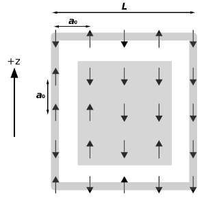
The Ising model has exact solutions in one and two dimensions, in contrast to the 3D cases all we know about which is through numerical simulations. Here, we aim at numerically solving the two- (2D) and three-dimensional (3D) Ising problems obeying Eq. 4 excluding the last term, namely with $B=0$ without loss of generality, using the Monte Carlo (MC) method [14]. To this end, we assume that the spins have primarily been aligned along the $z$ direction, as illustrated in Fig. 1 for a 2D, $5\times 5$, square lattice.

Figure 1: A 2D, $5\times 5$, square lattice of identical spins with the lattice constant $a_{0}$ and the length $L$—rendered in GIMP (version 2.8) [18]. Taking $a_{0}$ to be the length scale, $1+L\big{/}a_{0}$ gives the number of spins in each row or column. Only two possible space orientations (namely, $\pm z$) are assumed to be allowed, meaning spin–1/2 particles. The total number of spins is also $N=25$, out of which $N_{b}=16$ spins are on the border (indicated by the gray narrow band), and the rest, $N_{v}=9$ spins, are in the volume (the central gray area) of the system, showing that the ratio $N_{b}\big{/}N_{v}\simeq 1.77\gg 0$ is quite large, affecting dramatically the physics of the problem as well.

The minus sign behind $J$ in Eq. 4 indicates that any two neighboring spins prefer to be in the same direction. In other words, to maintain this minus, which is fundamental in order for the entire system to have a negative energy, both $\sigma_{i}$ and $\sigma_{j}$ must be either $+1$ or $-1$; otherwise, $\sigma_{i}.\sigma_{j}=-1$ leading as well to a positive total energy value for our bounded system. Therefore, any two neighboring spins tend to be parallel in either direction. It is also easy to infer that if the system is left to its own devices, namely in the absence of any external agitating factor such as magnetic fields (then $B=0$) or thermal fluctuations (then $T=0$), all spins tend to be parallel in either space orientation, and the minimum-energy $(E_{min})$ configuration is accordingly obtained. In such a case, the minimum number of microstates of the system is evidently $\Omega_{min}=2$ (all spins up or down), leading in turn to minimum entropy $(\mathcal{S}_{min}=k_{B}\ln\Omega_{min}=k_{B}\ln 2$; $k_{B}$ being the Boltzmann constant). Moreover, because $T=0$, minimum free energy $(F_{min})$ is also obtained according to the thermodynamic relation $F=E-T\mathcal{S}$. Evidently, any difference in the sign of neighboring spins increases the energy of the system.

Nevertheless, for $T>0$, minimum energy is not concurrent with minimum free energy due to $T\mathcal{S}>0$. To further clarify this point, we consider two microstates of the lattice of Fig. 1: one with all spins up, and the other with only one spin down. For the former, $\Omega=1$ and then $\mathcal{S}=k_{B}\ln 1=0$. For the latter, however, $\mathcal{S}=k_{B}\ln\left[N!\big{/}(N-1)!\right]=k_{B}\ln 25$, according to the fact that the only opposite (down) spin can be in any lattice point. The microstate with half of the spins up (or down) thus possesses both maximum entropy and zero magnetization $(M)$ simultaneously. As a result, $F_{min}$ is obtained when $T\mathcal{S}$ is maximum, namely when $\mathcal{S}$ is maximum, or for high enough temperature values that again lead to maximum entropy, or to $M=0$. It means that at high enough temperatures, the system lacks a net magnetization, and vice versa, as temperature decreases, $T\mathcal{S}$ becomes small, $F$ approaches $E$, and the system accordingly possesses a net, non-zero magnetization. According to this inverse correlation between $M$ and $T\mathcal{S}$, the former can then be viewed as an indication of order of the system, called as well the order parameter. At a critical temperature ($T_{c}$), the system undergoes a phase transition in a way that $M$ suddenly drops to zero; for $T<T_{c}$ the system is in the state in which all the spins are either up or down (minimum entropy), while for $T>T_{c}$ the system asymptotically moves to the state with half of the spins up or down (maximum entropy). As a result, this model features one of the most important phenomenon in physics, which is called spontaneous symmetry breaking [19]: at temperatures considerably higher than $T_{c}$, there exists an up-down spin symmetry, which spontaneously breaks into either spins-up or spins-down state as temperature approaches $T_{c}$.

Studying the behavior of the system in the vicinity of its critical point is indeed a basic problem in the theory of phase transition. Such a behavior is marked by the fact that various physical quantities of the system (e.g., the thermodynamic observables and/or their derivatives) possess singularities or discontinuities at the critical temperature. Notable examples of this type in the Ising model are the critical behaviors of the specific heat $(C_{v})$ and the magnetic susceptibility $(\chi)$. From statistical mechanics, such singularities are direct consequences of the fact that the correlation length $(\xi)$ of the system becomes infinitely large at $T_{c}$. This quantity is in fact a manifestation of the correlation between spin positions in the lattice. Due to such an infiniteness, the system becomes scale-free meaning that the asymptotic behaviors of the associated physical observables of the system near the critical point are given by power laws—say $M\sim(T_{c}-T)^{\delta}$, $\chi\sim|T_{c}-T|^{-\gamma}$, $C_{v}\sim|T_{c}-T|^{-\alpha}$, and $\xi\sim|T_{c}-T|^{-\nu}$, where $|T_{c}-T|$ means both $T_{c}-T$ and $T-T_{c}$ depending on the sign of $T_{c}-T$ at the neighborhood of $T_{c}$. As is seen, these power laws are characterized by the parameters $\alpha,\gamma,\delta$, and $\nu$, known as critical exponents, determining as well the qualitative nature of the critical behavior of the system.

2.1 Ensemble and phase space of the system

Assume that the original system of interest is a 2D square lattice with a total number $N$ of localized identical spins. Based on the fact that the standard statistical ensemble in MC simulations is the canonical ensemble [this is indeed due to the natural appearance of the equilibrium temperature in the Boltzmann weight factor $e^{-\beta E}$ ($\beta=1/k_{B}T$)], we accordingly consider a large ensemble consisting of many mental copies of the original system, being naturally enough in all sorts of possible configurations (microstates), including as well all possible states.

Considering this ensemble, the various systems will be in all sorts of possible microstates at any instant of time, consistent with the given macrostate which is common to all of them. In the phase space of the system, the corresponding picture involves a swarm of representative phase points, each of which for one member of the ensemble. In terms of dynamics, as the systems of the ensemble move continually between different microstates with time, the corresponding representative points also simultaneously move along their respective phase-space paths.

In the most general case, supposing the original system of interest to be a $D$-dimensional lattice with $N$ identical spins localized on the lattice points, the average of the thermodynamic observable $A$ pertaining to this system in say the canonical ensemble is then given by

$$\langle A\rangle=\bigg{[}\int A(q,p)e^{-\beta E(q,p)}d^{DN}q\hskip 1.42262ptd^{DN}p\bigg{]}\Bigg{/}\bigg{[}\int e^{-\beta E(q,p)}d^{DN}q\hskip 1.42262ptd^{DN}p\bigg{]},$$ (5)

which involves two many-dimensional integrals, $\big{(}d^{DN}q\hskip 1.42262ptd^{DN}p\big{)}$ is the volume element in the ($DN+DN=$) $2DN$-dimensional phase space, $q$ and $p$ are respectively the position and momentum coordinates, and $E(q,p)$ is the total energy of the system. Even, by taking into account the fact that interactions between the spins are velocity-independent (according to Eq. 4) and the momentum integrals could accordingly be separated off, carrying out integration in a $DN$-dimensional configuration space using usual numerical techniques is still quite impossible—$e^{-\beta E(q,p)}$ is in general the density of the phase-space representative points, which can also be more complicatedly a function of time. Resorting to MC methods, Eq. 5 accordingly turns into the simple unweighted average

$$\langle A\rangle=\frac{1}{M}\sum_{i=1}^{M}A({\mathfrak{q}}_{i})$$ (6)

where $M$ is the number of microstates ${\mathfrak{q}}_{i}$ within the sample $\{\mathfrak{q}\}$—a sample, here, is referred to as a set of microstates, which is in turn a subset of the ensemble.

2.2 The modified Monte Carlo scheme

In statistical mechanics, computer simulations involve two major categories, including molecular dynamics (MD) [20], and MC. In equilibrium statistical mechanics, an MC simulation uses pseudorandom number generators to sample the ensemble of the system according to the equilibrium probability distribution

$$\mathcal{P}(\mathfrak{q})=\frac{e^{-\beta E(\mathfrak{q})}}{\sum_{\mathfrak{q^{\prime}}}e^{-\beta E(\mathfrak{q^{\prime}})}},$$ (7)

where the summation is carried out over all members of the set $\{\mathfrak{q^{\prime}}\}$. In a modified MC scheme devised by Metropolis et al. [15], an MC simulation samples configurations (microstates) according to the Boltzmann weight factor $e^{-\beta E}$ and then weights them evenly, instead of drawing a sample randomly and then weighting them by $e^{-\beta E}$. The former, referred to as importance sampling, is indeed more optimized and computationally cost-effective compared to the latter simple-minded random sampling, and brings about a remarkable computational efficiency because according to which, all microstates within the sample are chosen with a probability $e^{-\beta E}$. Therefore, expectation values of the thermodynamic observables could simply be calculated by Eq. 6.

2.3 The Metropolis algorithm

Random walk in the sampling space, i.e., selecting a random microstate $\mathfrak{q}$ from the set $\{\mathfrak{q}\}$ with a probability distribution approaching Eq. 7, is accomplished by the Metropolis algorithm. Using Eq. 7, for two consecutive states $\mathfrak{q}$ and $\mathfrak{q^{\prime}}$ (the system moves from the former to the latter state in its phase space), it is obtained that

$$\frac{\mathcal{P}(\mathfrak{q^{\prime}})}{\mathcal{P}(\mathfrak{q})}=e^{-\beta\big{[}E(\mathfrak{q^{\prime}})-E(\mathfrak{q})\big{]}}=e^{-\beta\Delta E}.$$

This factor, as we show later on, lies at the heart of the Metropolis algorithm, and governs as well the random walks on the lattice. One important feature of this ratio is that it depends only on the energy difference between any two states, therefore, there is no need to have energies of all the microstates as included in the denominator of Eq. 7 as the canonical partition function of the system.

The Metropolis algorithm is accomplished in the following five steps:

• Step I. Change the present microstate $\mathfrak{q}$ of the system to another randomly chosen state $\mathfrak{q^{\prime}}$. In an Ising problem, this is equivalent to flipping a randomly selected spin. Since the total energy $(E)$ explicitly appears in the Boltzmann weight factor, it must then be an explicit function of the microstate of the system in a way that change in $\mathfrak{q}$ directly changes $E$.

• Step II. Calculate the energy difference $\Delta E=E(\mathfrak{q^{\prime}})-E(\mathfrak{q})$. If $\Delta E\leq 0$, then $E(\mathfrak{q^{\prime}})\leq E(\mathfrak{q})$ [therefore $\mathcal{P}(\mathfrak{q^{\prime}})\geq\mathcal{P}(\mathfrak{q})$] which is a desired result due to bringing about a less total energy compared to the previous state of the system, the change must then be accepted. In contrast, $\Delta E>0$ is not desired, nevertheless, we do not ignore this case and accept the related change with probability $e^{-\beta\Delta E}$. And how one can accept a change with a probability? The most familiar way is undoubtedly to use a die. As an illustration, assume you aim to accept a change or make a selection with probability $P_{0}=0.25$. You accordingly have to design a tetrahedron, pyramid-shape die with four equilateral triangular faces. Indeed, when we use coins or cubic dice, we are making selections with probabilities 0.5 and 0.167, respectively. Here, because $\Delta E>0$, $e^{-\beta\Delta E}$ is always between 0 and 1, and we can then design a computational die with $e^{+\beta\Delta E}$ sides. Since this exponential almost never results in a uniform die due to being inherently any real number—in other words, choosing a (real) random number between 0 and 1 almost never would be equal to a specific value of $e^{-\beta\Delta E}$ due to the never-happening match between their decimals—a more general, less stringent condition is then to accept the change with a probability less than $e^{-\beta\Delta E}$. This condition can indeed be justified according to the fact that the change with $\Delta E>0$ is not a desired one and we basically tend to get rid of this. As a result, being $rand()$ a random number between 0 and 1 as a probability, if $rand()<e^{-\beta\Delta E}$, then the change is accepted. Albeit seemingly evident, it should be useful to note that producing one random number using a pseudorandom number generator is equivalent to one throw of our computational die.

• Step III. Perform steps I and II once for each spin in the system (i.e., one spin at a time). The spins are usually selected randomly to ensure detailed balance [16, 17]. Steps I through III also define one MC sweep.

• Step IV. Repeat steps I through III for a number (eqstp in the codes) of MC sweeps in order for the entire system to be equilibrated. This value cannot be indeed estimated a priori. As a result, for an arbitrary value of temperature in the temperature loop of the code, one has to plot the total energy of the system at each step of equilibration and then check whether convergence is achieved.

• Step V. Repeat steps I through III for a number (mcstp in the codes of Sec. 3.4) of MC sweeps.

2.4 Ergodicity

In both major classes of computer simulation in statistical mechanics, MD and MC, the condition of being ergodic is cardinal, without which the simulations are not reliable to calculate the thermodynamic averages of interest. In the present MC algorithm, since all spins are equally likely to be chosen with finite probabilities, a large enough number of random moves would accordingly give the chance to all of them to be flipped, showing the ergodicity of the method. In other words, any microstate of the system can be reached from any other. More importantly, if we make a change in all the systems of the ensemble, and define $P_{\mathfrak{q}\rightarrow\mathfrak{q^{\prime}}}$ as the probability of a system to be carried out from state $\mathfrak{q}$ to $\mathfrak{q^{\prime}}$ caused by that change, ergodicity guarantees that

$$P_{\mathfrak{q}\rightarrow\mathfrak{q^{\prime}}}=P_{\mathfrak{q^{\prime}}\rightarrow\mathfrak{q}},$$ (8)

because all possible microstates are equally likely to happen.

2.5 Canonical distribution of the ensemble

The initial distribution of the ensemble, involving many copies of the original system, is evidently random: ${\mathcal{M}}_{\mathfrak{q}}$ systems in state $\mathfrak{q}$, ${\mathcal{M}}_{\mathfrak{q^{\prime}}}$ systems in state $\mathfrak{q^{\prime}}$, ${\mathcal{M}}_{\mathfrak{q^{\prime\prime}}}$ systems in state ${\mathfrak{q^{\prime\prime}}}$, and so on. We indeed aim at approaching an ensemble in which the distribution of any configuration (microstate) ${\mathfrak{q}}_{i}$ is given by Eq.7. The why of this goal is that the final ensemble will be accordingly composed of low-energy configurations, namely the states that are most probable to occur in Nature, including as well the ground state of the system. This, in fact, is a kind of importance sampling, and once the probability distribution of our ensemble approaches Eq.7, we are then allowed to weight them evenly, which exactly means that the simulation averages of the thermodynamic observables are simply given by Eq. 6.

We now assume that ${\mathcal{M}}_{\mathfrak{q}}$ is the number of systems of the ensemble that are in state $\mathfrak{q}$, and $E(\mathfrak{q})>E(\mathfrak{q^{\prime}})$, $\mathfrak{q^{\prime}}$ being another state. Therefore, transition from $\mathfrak{q}$ to $\mathfrak{q^{\prime}}$ is allowed due to bringing about a lower energy, and the total number of systems moving from $\mathfrak{q}$ to $\mathfrak{q^{\prime}}$ is simply given by ${\mathcal{M}}_{\mathfrak{q}}P_{\mathfrak{q}\rightarrow\mathfrak{q^{\prime}}}$. The number of systems moving from $\mathfrak{q^{\prime}}$ to $\mathfrak{q}$ is also

$$\mathcal{N}(\mathfrak{q^{\prime}}\rightarrow\mathfrak{q})={\mathcal{M}}_{\mathfrak{q^{\prime}}}P_{\mathfrak{q^{\prime}}\rightarrow\mathfrak{q}}e^{-\beta\Delta E}={\mathcal{M}}_{\mathfrak{q^{\prime}}}P_{\mathfrak{q}\rightarrow\mathfrak{q^{\prime}}}e^{-\beta[E(\mathfrak{q})-E(\mathfrak{q^{\prime}})]},$$

obtained according to the Metropolis algorithm (step II), and by using Eq. 8. As a result, the net difference between the number of systems moving from $\mathfrak{q}$ to $\mathfrak{q^{\prime}}$ and that of the reverse direction is then

$$\mathcal{N}(\mathfrak{q}\rightarrow\mathfrak{q^{\prime}})-\mathcal{N}(\mathfrak{q^{\prime}}\rightarrow\mathfrak{q})={\mathcal{M}}_{\mathfrak{q}}P_{\mathfrak{q}\rightarrow\mathfrak{q^{\prime}}}-{\mathcal{M}}_{\mathfrak{q^{\prime}}}P_{\mathfrak{q}\rightarrow\mathfrak{q^{\prime}}}e^{-\beta[E(\mathfrak{q})-E(\mathfrak{q^{\prime}})]}=P_{\mathfrak{q}\rightarrow\mathfrak{q^{\prime}}}\Big{(}{\mathcal{M}}_{\mathfrak{q}}-{\mathcal{M}}_{\mathfrak{q^{\prime}}}e^{-\beta[E(\mathfrak{q})-E(\mathfrak{q^{\prime}})]}\Big{)}.$$

From the Metropolis algorithm, it can be inferred that more systems will eventually move from state $\mathfrak{q}$ to $\mathfrak{q^{\prime}}$ on average, according to our previous assumption $E(\mathfrak{q^{\prime}})<E(\mathfrak{q})$, therefore,

$$\mathcal{N}(\mathfrak{q}\rightarrow\mathfrak{q^{\prime}})>\mathcal{N}(\mathfrak{q^{\prime}}\rightarrow\mathfrak{q})\Longrightarrow\mathcal{N}(\mathfrak{q}\rightarrow\mathfrak{q^{\prime}})-\mathcal{N}(\mathfrak{q^{\prime}}\rightarrow\mathfrak{q})>0\Longrightarrow{\mathcal{M}}_{\mathfrak{q}}-{\mathcal{M}}_{\mathfrak{q^{\prime}}}e^{-\beta[E(\mathfrak{q})-E(\mathfrak{q^{\prime}})]}>0$$

$$\Longrightarrow{\mathcal{M}}_{\mathfrak{q}}>{\mathcal{M}}_{\mathfrak{q^{\prime}}}\frac{e^{-\beta E(\mathfrak{q})}}{e^{-\beta E(\mathfrak{q^{\prime}})}}=\bigg{(}\frac{e^{-\beta E(\mathfrak{q^{\prime}})}}{{\mathcal{M}}_{\mathfrak{q^{\prime}}}}\bigg{)}^{-1}e^{-\beta E(\mathfrak{q})}\Longrightarrow{\mathcal{M}}_{\mathfrak{q}}=c_{0}\bigg{(}\frac{e^{-\beta E(\mathfrak{q^{\prime}})}}{{\mathcal{M}}_{\mathfrak{q^{\prime}}}}\bigg{)}^{-1}e^{-\beta E(\mathfrak{q})}\Longrightarrow{\mathcal{M}}_{\mathfrak{q}}\propto e^{-\beta E(\mathfrak{q})},$$

meaning that the ensemble will approach the canonical distribution—here, $c_{0}$ is some constant, and the ratio with the exponent $(-1)$ is also a detailed average, namely the probability of being in microstate $\mathfrak{q^{\prime}}$ averaged over all the systems that are in this state.

3 Simulation details

3.1 Initialization

The initial state of the system can be a random distribution of $(\pm 1)$ (associated with the two eigenvalues of $\hat{\sigma}_{z}$). It is also quite reasonable to start with a minimum-entropy configuration, such as the spins-up microstate, as we do here. We therefore store the number $N$ of $(+1)$s as elements of an array, which are then loaded into the computer memory once the code is run (one can also store them into an input file, but it is indeed redundant due to the fact that the initial configuration of the system after few MC sweeps is entirely lost and will not be reversible/retrievable anymore).

3.2 Energy

The total energy of the system, according to Eq. 4 (with $B=0$), is given by

$$-E\Big{/}J=2\sum_{i>j}\sigma_{i}.\sigma_{j}=\sum_{i=1}\sum_{j=1}\sigma_{i}.\sigma_{j},$$ (9)

according to which $J$ can be simply chosen as the unit of energy ($E\big{/}J$ is dimensionless). The energy difference is also calculated as follows. Assume in an MC sweep, the spin $s_{ij}$ is supposed to be flipped. Before flip (for a 2D lattice) we have

$$E(\mathfrak{q})=E_{0}+s_{ij}\Big{(}s_{i+1,j}+s_{i-1,j}+s_{i,j+1}+s_{i,j-1}\Big{)},$$

while after flip,

$$E(\mathfrak{q^{\prime}})=E_{0}-s_{ij}\Big{(}s_{i+1,j}+s_{i-1,j}+s_{i,j+1}+s_{i,j-1}\Big{)},$$

where $E_{0}$ is the energy contribution of all the spins excluding $s_{ij}$ and its four nearest neighbors. As a result, the energy difference is given by

$$\Delta E=E(\mathfrak{q^{\prime}})-E(\mathfrak{q})=-2s_{ij}\Big{(}s_{i+1,j}+s_{i-1,j}+s_{i,j+1}+s_{i,j-1}\Big{)}.$$

An alternative method (as in code5.py) uses the fact that this expression can also be written as

$$\Delta E\in\{-8,-4,0,4,8\},$$ (10)

therefore, one can easily compute $e^{-\beta\Delta E}$ for this set, store them in a five-element array, and then call them according to case.

3.3 Periodic boundary conditions

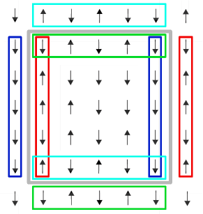
Hamiltonians involving many-body interactions are appeared in almost all physics, raising a quite important question as to how to treat the particles lying at the boundary of the system. As an illustration, these boundary particles, compared to the rest lying within the volume of the system, would accordingly experience only half of the interactions involved if the system is entirely immersed in say vacuum. In the thermodynamic limit (i.e., in macroscopic systems) the number $N_{b}$ of these boundary particles is absolutely negligible compared to the number $N_{v}$ of particles lying within the volume, therefore they do not affect the results. Nevertheless, the ratio $N_{b}\big{/}N_{v}$ is quite considerable (this is sometimes referred to as the finite-size effect) in all computer simulations of systems of particles due to the fact that simulating only small-scale systems several orders of magnitude smaller than their macroscopic analogues, as a consequence of limited computational power, is indeed feasible. A clear illustration of such systems has previously been shown in Fig. 1 in that most of the particles lay on the border. The question then arises: how is it possible to derive, or at least estimate approximately, different properties of interest pertaining to a given macroscopic system by only simulating a microscopic part of it? To do so, also to minimize the finite-size effect, a widely-used computational trick is called periodic boundary conditions—other types of boundary conditions are also possible, such as antiperiodic, free, etc. As an illustration, it is quite routine in computational solid state physics to calculate electronic structures of nanoscale materials [21, 22, 23, 24] using only their unit-cell information and then by applying the Born–von Karman periodic boundary conditions [25]. In the Ising model, as in MD simulations [26, 27, 28], it is assumed that the original system (the primary cell) is periodically replicated along the two spacial directions (or in the three directions for 3D problems) to form a macroscopic lattice [29]. Since only nearest-neighbor interactions are included in the Hamiltonian of the model (Eq. 4), the macroscopic lattice generated by replication, also involving an infinitely large number of particles, is simply scaled down to the original system plus its four nearest-neighbor rows and columns of spins, as illustrated in Fig. 2. Such a computational technique considerably reduces the finite-size effect particularly as the number of particles of the system increases.

Figure 2: The original system of Fig. 1 demarcated by the gray square, and its four nearest-neighbor rows and columns of spins separated off from the four neighboring image cells. Rectangles with identical colors are evidently of the same spin patterns.

3.4 Computer codes

We present five computer codes—code1.py, code2.f90, code3.py, code4.f90, and code5.py—written in both Python [30] (with .py suffix) and Fortran [31] (with .f90 suffix). The first two codes simulate a 2D problem, the next two solve a 3D problem, and the last one simulates a 2D lattice in that the energy difference is calculated according to Eq. 10. To run the codes, say code1.py, copy it into a text editor, save it with the same name and suffix, and run in the Linux command-line interface (CLI): python3 code1.py. To run the Fortran codes (say code2.f90), do the same and run: gfortran code2.f90 && ./a.out—one may also replace gfortran with ifort, or mpif90, or any other Fortran compiler. After the run is finished, the file output.txt is generated which contains six columns including, in order from left to right, the inverse temperature $\big{(}\beta=1\big{/}k_{B}T\big{)}$, temperature $(T)$, mean energy $\big{(}\langle E\rangle\big{/}J\big{)}$, mean magnetization $\big{(}\langle M\rangle\big{)}$, specific heat $\big{(}\langle C_{v}\rangle\big{/}k_{B}\big{)}$, and zero-field magnetic susceptibility ($\langle\chi\rangle$ per unit volume)—$\langle...\rangle$ means average over both the total number of spins and number of nearest-neighbors (4 for 2D and 6 for 3D problems). All the codes were written using a function-based programming style (in contrast to the simple-minded top-down design). The temperature range $([0.5,10])$ has been chosen so as to include the analytic critical temperature of the 2D system, namely $k_{B}T_{c}\big{/}J=2\big{/}\tanh^{-1}(1/\sqrt{2})=2.269185$, which is an asymptotic value and is approached only in the limit $N\longrightarrow\infty$. As a result, we have used $T_{c}=2.50$ for a $20\times 20$ lattice, obtained by trial and error, for plotting the output of code2.f90. Comparing the simulation times of one given system obtained by both Fortran and Python codes also reveals the fact that the former programming language is much more faster than the latter in scientific computing and simulation.

3.4.1 code1.py

⬇

1#!/usr/bin/python3

2import random

3import numpy as np

4from numpy.random import rand

5#-------------------------------------------

6L = 5 # Size of the square lattice

7mcstp = 100 # Number of MC sweep

8eqstp = 100 # Number of MC sweep for equilibration

9D = 2 # Lattice dimension

10N = L**D # Number of spins

11NN = 4 # Number of nearest-neighbors

12T_0 = 0.5 # Initial temperature

13T_f = 10.0 # Final temperature

14dT = 0.1 # Temperature step

15#----------------------------------

16c = 0 # Counter

17T = T_0 # Temperature initialization

18norm = 1./(mcstp*N*NN)

19nr2 = norm/mcstp

20#---------------

21def INIT(L):

22 """ Generates initial confuguration (cfg): all spins up """

23 cfg = np.random.randint(1, size = (L, L)) + 1

24 return cfg

25#--------------------------

26def METROPOLIS(spin, beta):

27 """The Metropolis algorithm"""

28 for i in range(L):

29 for j in range(L):

30 x = np.random.randint(0, L) # X coordinate

31 y = np.random.randint(0, L) # Y coordinate

32 s = spin[x, y]

33 # Periodic boundary conditions --------------

34 R = spin[(x + 1)%L, y] + spin[x, (y + 1)%L] \

35 + spin[(x - 1)%L, y] + spin[x, (y - 1)%L]

36 #--------------------------------------------

37 dE = 2*s*R # Energy difference

38 if dE < 0.:

39 s *= -1 # Flips the spin

40 elif rand() < np.exp(-dE*beta): # Throws the die

41 s *= -1 # Flips the spin

42 spin[x, y] = s # Returns the spin without flipping

43 return spin

44#--------------------------

45def CALCULATE_ENERGY(spin):

46 """Computes energy"""

47 En = 0. # Energy

48 for x in range(len(spin)):

49 for y in range(len(spin)):

50 S = spin[x, y]

51 # Periodic boundary conditions --------------

52 R = spin[(x + 1)%L, y] + spin[x, (y + 1)%L] \

53 + spin[(x - 1)%L, y] + spin[x, (y - 1)%L]

54 #--------------------------------------------

55 En -= S*R

56 return En

57#---------------------------------

58def CALCULATE_MAGNETIZATION(spin):

59 """Computes magnetization"""

60 mgnt = np.sum(spin) # Magnetization

61 return mgnt

62#-----------------------------------

63# Opens the output file "output.txt"

64# containing beta (B= 1/k_{B}T),

65# temperature (T), and the mean values of energy (E),

66# magnetization (M), specific heat (C_v),

67# and susceptibility (Chi) of the system

68# at every temperature step.

69g = open(’output.txt’, ’w’)

70g.write(’# T^{-1} T E M C_v Chi\n’)

71g.write(’#======= ======== ======== ======== ======== ========\n’)

72#--------------------------------------------------

73while T <= T_f: # Temperature loop (main loop)

74 T += dT

75 summ = [0, 0, 0, 0] # Accumulators

76 spin = INIT(L)

77 c = c + 1

78 B = 1./T; B2 = B*B

79 for sweep in range(eqstp): # Equilibration loop

80 METROPOLIS(spin, B)

81#---------------------------------------------

82 for sweep in range(mcstp): # Main MC loop

83 METROPOLIS(spin, B)

84 E = CALCULATE_ENERGY(spin)

85 M = CALCULATE_MAGNETIZATION(spin)

86 #---------------------------------

87 summ[0] += E # E accumulator

88 summ[1] += E*E # E^2 accumulator

89 summ[2] += M # M accumulator

90 summ[3] += M*M # M^2 accumulator

91#-------------------------------------------------

92# Thermodynamic averages at each temperature step

93 mean_E = summ[0]*norm # Mean E

94 mean_M = summ[2]*norm # Mean M

95 C_v = (norm*summ[1] - nr2*summ[0]*summ[0])*B2 # Specific heat (C_v)

96 chi = (norm*summ[3] - nr2*summ[2]*summ[2])*B # Susceptibility (Chi)

97 g.write(’%f %f %f %f %f %f\n’ \

98 %(B, T, mean_E, mean_M, C_v, chi))

99 print(’>>> Temperature step %d’ %(c))

3.4.2 code2.f90

⬇

1module SHARED_DATA

2implicit none

3save

4integer i, j ! Loop counters

5integer x, y ! Position coordinates

6integer up, down, right, left

7integer, parameter :: L = 5 ! Size of the quare lattice

8integer, parameter :: D = 2 ! Lattice dimension

9integer, parameter :: N = L**D ! Number of spins

10integer, parameter :: mcstp = 100 ! Monte Carlo sweeps

11integer, parameter :: eqstp = 100 ! Monte Carlo sweeps for equilibration

12integer, parameter :: NN = 4 ! Number of nearest-neighbors

13real, parameter :: T_0 = 0.5 ! Initial temperature

14real, parameter :: T_f = 10.0 ! Final temperature

15real, parameter :: norm = 1./(mcstp*N*NN)

16real, parameter :: nr2 = norm/mcstp

17real, parameter :: dT = 0.1 ! Temperature step

18end module

19!-------------------------------

20subroutine METROPOLIS(sp, beta)

21! The Metropolis algorithm"""

22use SHARED_DATA

23implicit none

24integer, intent(inout) :: sp(L, L) ! Spin

25real, intent(in) :: beta ! = 1/k_{B}T

26integer s ! Box for spin

27real R

28integer dE ! Energy difference

29real rand, x0, y0 ! Random numbers

30do i = 1, L

31 do j = 1, L

32 call random_number(x0)

33 call random_number(y0)

34 x = int(1 + (L - 1)*x0)

35 y = int(1 + (L - 1)*y0)

36 s = sp(x, y)

37 ! Periodic boundary conditions

38 if (x == 1) then

39 left = sp(L, y)

40 right = sp(2, y)

41 else if (x == L) then

42 left = sp(L - 1, y)

43 right = sp(1, y)

44 else

45 left = sp(x - 1, y)

46 right = sp(x + 1, y)

47 end if

48 if (y == 1) then

49 up = sp(x, 2)

50 down = sp(x, L)

51 else if (y == L) then

52 up = sp(x, 1)

53 down = sp(x, L - 1)

54 else

55 up = sp(x, y + 1)

56 down = sp(x, y - 1)

57 end if ! End of periodic boundary conditions

58 R = up + down + right + left

59 dE = 2*s*R

60 call random_number(rand)

61 if (dE < 0.) then

62 s = -s ! Flips the spin

63 else if (rand < exp(-dE*beta)) then ! Throws the die

64 s = -s ! Flips the spin

65 end if

66 sp(x, y) = s ! Returns the spin without flipping

67 enddo

68enddo

69end subroutine METROPOLIS

70!-----------------------------------

71real function CALCULATE_ENERGY(sp1)

72use SHARED_DATA

73implicit none

74integer, intent(in) :: sp1(L, L) ! Spin

75real En, R

76En = 0. ! Energy initialization

77do x = 1, L

78 do y = 1, L

79 if (x == 1) then

80 left = sp1(L, y)

81 right = sp1(2, y)

82 else if (x == L) then

83 left = sp1(L - 1, y)

84 right = sp1(1, y)

85 else

86 left = sp1(x - 1, y)

87 right = sp1(x + 1, y)

88 end if

89 if (y == 1) then

90 up = sp1(x, 2)

91 down = sp1(x, L)

92 else if (y == L) then

93 up = sp1(x, 1)

94 down = sp1(x, L - 1)

95 else

96 up = sp1(x, y + 1)

97 down = sp1(x, y - 1)

98 end if

99 R = up + down + right + left

100 En = En - sp1(x, y)*R

101 enddo

102enddo

103CALCULATE_ENERGY = En ! Energy

104end function

105!------------------------------------------

106real function CALCULATE_MAGNETIZATION(sp2)

107use SHARED_DATA

108implicit none

109integer, intent(in) :: sp2(L, L) ! Spin

110CALCULATE_MAGNETIZATION = sum(sp2) ! Magnetization

111end function

112!------------------------------

113program ising ! Main program

114use SHARED_DATA

115implicit none

116integer sweep ! Loop counter

117real T, B, B2 ! Temperature, beta = 1/k_{B}T, beta^2

118real summ0, summ1, summ2, summ3, summ4 ! Accumulators

119real E, M ! energy, magnetization

120real CALCULATE_ENERGY, CALCULATE_MAGNETIZATION ! External functions

121real mean_E, mean_M, C_v, chi ! Mean E, mean M, specific heat, susceptibility

122integer :: spin(L, L) = 1 ! Initial configuration: all spins up

123integer c ! Counter

124open(1, file = ’output.txt’) ! Output file: beta, T, E, M, Cv, chi

125open(2, file = ’eqltst.txt’) ! Output file for equilibration test

126T = T_0 ! Temperature initialization

127c = 0

12810 format (6f12.6)

129write(1, *)"# T^{-1} T E M C_v Chi"

130write(1, *)"# ======== ======== ======== ======== ======== ========"

131do while (T <= T_f) ! Temperature loop (main loop)

132 T = T + dT

133 c = c + 1

134 summ0 = 0.; summ1 = 0.; summ2 = 0.; summ3 = 0. ! Initializing accumulators

135 B = 1./T; B2 = B*B ! Beta, beta^2

136 do sweep = 1, eqstp ! Equilibration loop

137 call METROPOLIS(spin, B)

138 ! Activate the following 4 comment lines

139 ! (from the line 142 to 145) to check whether

140 ! equilibration is achieved for a given

141 ! temperature (here, T = 2).

142 ! To this end, plot eqltst.txt.

143 !E = CALCULATE_ENERGY(spin)

144 !if (int(T) == 2) then

145 ! write(2,*) step, E

146 !end if

147 enddo

148 !-------------------------------------

149 do sweep = 1, mcstp ! Main MC loop

150 call METROPOLIS(spin, B)

151 E = CALCULATE_ENERGY(spin)

152 M = CALCULATE_MAGNETIZATION(spin)

153 summ0 = summ0 + E ! E accumulator

154 summ1 = summ1 + E*E ! E^2 accumulator

155 summ2 = summ2 + M ! M accumulator

156 summ3 = summ3 + M*M ! M^2 accumulator

157 end do

158 !--------------------------------------------------

159 ! Thermodynamic averages at each temperature value

160 mean_E = summ0*norm ! Mean energy

161 mean_M = summ2*norm ! Mean magnetization

162 C_v = (norm*summ1 - nr2*summ0*summ0)*B2 ! Specific heat

163 chi = (norm*summ3 - nr2*summ2*summ2)*B ! Susceptibility

164 write(1, 10)B, T, mean_E, mean_M, C_v, chi

165 write(*, *)" >>> Temperature step", c

166end do

167end program

3.4.3 code3.py

⬇

1#!/usr/bin/python3

2import random

3import numpy as np

4from numpy.random import rand

5#--------------------------------------------

6L = 4 # Size of the square lattice

7D = 3 # Lattice dimension

8mcstp = 100 # Number of MC sweeps

9eqstp = 100 # Number of MC sweeps for equilibration

10N = L**D # Number of spins

11NN = 6 # Number of nearest-neighbors

12T_0 = 0.5 # Initial temperature

13T_f = 10.0 # Final temperature

14dT = 0.1 # Temperature step

15c = 0 # Counter

16T = T_0 # Temperature initialization

17norm = 1./(mcstp*N*NN)

18nr2 = norm/mcstp

19#---------------

20def INIT(L):

21 """Initial confuguration (cfg): all spins up"""

22 cfg = np.random.randint(1, size = (L, L, L)) + 1

23 return cfg

24#--------------------------

25def METROPOLIS(spin, beta):

26 """The Metropolis algorithm"""

27 for i in range(L):

28 for j in range(L):

29 for k in range(L):

30 x = np.random.randint(0, L) # X coordinate

31 y = np.random.randint(0, L) # Y coordinate

32 z = np.random.randint(0, L) # Z coordinate

33 s = spin[x, y, z] # Spin

34 # Periodic boundary conditions --------------------

35 R = spin[(x + 1)%L, y, z] + spin[x, (y + 1)%L, z] \

36 + spin[(x - 1)%L, y, z] + spin[x, (y - 1)%L, z] \

37 + spin[x, y, (z - 1)%L] + spin[x, y, (z + 1)%L]

38 #----------------------------------------------

39 dE = 2*s*R # Energy difference

40 if dE < 0.:

41 s *= -1 # Flips the spin

42 elif rand() < np.exp(-dE*beta): # Throws the die

43 s *= -1 # Flips the spin

44 spin[x, y, z] = s # Returns the spin without flipping

45 return spin

46#--------------------------

47def CALCULATE_ENERGY(spin):

48 """computes energy"""

49 En = 0.

50 for x in range(len(spin)):

51 for y in range(len(spin)):

52 for z in range(len(spin)):

53 S = spin[x, y, z] # Spin

54 # Periodic boundary conditions --------------------

55 R = spin[(x + 1)%L, y, z] + spin[x, (y + 1)%L, z] \

56 + spin[(x - 1)%L, y, z] + spin[x, (y - 1)%L, z] \

57 + spin[x, y, (z - 1)%L] + spin[x, y, (z + 1)%L]

58 #----------------------------------------------

59 En -= S*R # Energy

60 return En

61#----------------------------------

62def CALCULATE_MAGNETIZATION(spin):

63 """computes magnetization"""

64 mgnt = np.sum(spin) # Magnetization

65 return mgnt

66#-----------------------------------

67# Opens the output file "output.txt"

68# containing beta (B= 1/k_{B}T),

69# temperature (T), and the mean values of energy (E),

70# magnetization (M), specific heat (C_v),

71# and susceptibility (Chi) of the system

72# at every temperature.

73g = open(’output.txt’, ’w’)

74g.write(’# T^{-1} T E M C_v Chi\n’)

75g.write(’#======= ======== ======== ======== ======== ========\n’)

76#-----------------------------------------------

77while T <= T_f: # Temperature loop (main loop)

78 T += dT

79 s = [0, 0, 0, 0] # Initializing accumulators

80 spin = INIT(L) # Loads initial configuration

81 c = c + 1

82 B = 1./T; B2 = B*B

83 for sweep in range(eqstp): # Equilibration loop

84 METROPOLIS(spin, B)

85 #------------------------------------------

86 for sweep in range(mcstp): # Main MC loop

87 METROPOLIS(spin, B)

88 E = CALCULATE_ENERGY(spin)

89 M = CALCULATE_MAGNETIZATION(spin)

90 #---------------------------------

91 s[0] += E # E accumulator

92 s[1] += E*E # E^2 accumulator

93 s[2] += M # M accumulator

94 s[3] += M*M # M^2 accumulator

95 #---------------------------------------------

96 # Thermodynamic averages at each temperature step

97 mean_E = s[0]*norm # Mean energy

98 mean_M = s[2]*norm # Mean magnetization

99 C_v = (norm*s[1] - nr2*s[0]*s[0])*B2 # Specific heat

100 chi = (norm*s[3] - nr2*s[2]*s[2])*B # Susceptibility

101 g.write(’%f %f %f %f %f %f\n’ \

102 %(B, T, mean_E, mean_M, C_v, chi))

103 print(’>>> Temperature step %d’ %(c))

3.4.4 code4.f90

⬇

1module shared_data

2implicit none

3save

4integer i, j, k ! Loop counters

5integer x, y, z ! Spins’ position coordinates

6integer up, down, right, left, above, below

7integer, parameter :: L = 4 ! Size of the square lattice

8integer, parameter :: D = 3 ! Lattice dimension

9integer, parameter :: N = L**D ! Number of spins

10integer, parameter :: NN = 6 ! Number of nearest-neighbors

11integer, parameter :: mcstp = 100 ! Number of Monte Carlo sweeps

12integer, parameter :: eqstp = 100 ! Number of Monte Carlo sweeps for equilibration

13real, parameter :: T_0 = 0.5 ! Initial temperature

14real, parameter :: T_f = 10.0 ! Final temperature

15real, parameter :: norm = 1./(mcstp*N*NN)

16real, parameter :: nr2 = norm/mcstp

17real, parameter :: dT = 0.1 ! Temperature step

18end module

19!--------------------------------

20subroutine METROPOLIS(spin, beta)

21! The Metropolis algorithm

22use shared_data

23implicit none

24integer, intent(inout) :: spin(L, L, L) ! Spins

25real, intent(in) :: beta ! Beta = 1/kB*T

26integer s ! Box for spin

27real R

28real dE ! Energy difference

29real x0, y0, z0, rand ! Random numbers

30do i = 1, L

31 do j = 1, L

32 do k = 1, L

33 call random_number(x0)

34 call random_number(y0)

35 call random_number(z0)

36 x = int(1 + (L - 1)*x0) ! X coordinate

37 y = int(1 + (L - 1)*y0) ! Y coordinate

38 z = int(1 + (L - 1)*z0) ! Z coordinate

39 s = spin(x, y, z) ! Spin

40 ! Periodic boundary conditions

41 if (x == 1) then

42 left = spin(L, y, z)

43 right = spin(2, y, z)

44 else if (x == L) then

45 left = spin(L - 1, y, z)

46 right = spin(1, y, z)

47 else

48 left = spin(x - 1, y, z)

49 right = spin(x + 1, y, z)

50 end if

51 if (y == 1) then

52 up = spin(x, 2, z)

53 down = spin(x, L, z)

54 else if (y == L) then

55 up = spin(x, 1, z)

56 down = spin(x, L - 1, z)

57 else

58 up = spin(x, y + 1, z)

59 down = spin(x, y - 1, z)

60 end if

61 if (z == 1) then

62 above = spin(x, y, 2)

63 below = spin(x, y, L)

64 else if (z == L) then

65 above = spin(x, y, 1)

66 below = spin(x, y, L - 1)

67 else

68 above = spin(x, y, z + 1)

69 below = spin(x, y, z - 1)

70 end if ! End of periodic boundary conditions

71 R = up + down + right + left + above + below

72 dE = 2*s*R ! Energy difference

73 call random_number(rand) !Throws the die

74 if (dE < 0.) then

75 s = -s ! Flips the spin

76 elseif (rand < exp(-dE*beta)) then

77 s = -s ! Flips the spin

78 endif

79 spin(x, y, z) = s ! Returns the spin without flipping

80 enddo

81 enddo

82enddo

83end subroutine METROPOLIS

84!-----------------------------------

85real function CALCULATE_ENERGY(spin)

86use shared_data

87implicit none

88integer, intent(in) :: spin(L, L, L)

89real En, R

90En = 0. ! Energy initialization

91do x = 1, L

92 do y = 1, L

93 do z = 1, L

94 ! Periodic boundary conditions

95 if (x == 1) then

96 left = spin(l, y, z)

97 right = spin(2, y, z)

98 else if (x == L) then

99 left = spin(l - 1, y, z)

100 right = spin(1, y, z)

101 else

102 left = spin(x - 1, y, z)

103 right = spin(x + 1, y, z)

104 end if

105 if (y == 1) then

106 up = spin(x, 2, z)

107 down = spin(x, L, z)

108 else if (y == L) then

109 up = spin(x, 1, z)

110 down = spin(x, L - 1, z)

111 else

112 up = spin(x, y + 1, z)

113 down = spin(x, y - 1, z)

114 end if

115 if (z == 1) then

116 above = spin(x, y, 2)

117 below = spin(x, y, L)

118 else if (z == L) then

119 above = spin(x, y, 1)

120 below = spin(x, y, L - 1)

121 else

122 above = spin(x, y, z + 1)

123 below = spin(x, y, z - 1)

124 end if

125 R = up + down + right + left + above + below

126 En = En - spin(x, y, z)*R ! Energy accumulation

127 enddo

128 enddo

129enddo

130CALCULATE_ENERGY = En ! Energy

131end function

132!------------------------------------------

133real function CALCULATE_MAGNETIZATION(spin)

134use shared_data

135implicit none

136integer, intent(in) :: spin(L, L, L) ! Spin

137CALCULATE_MAGNETIZATION = sum(spin) ! Magnetization

138end function

139!------------------------------

140program ising ! Main program

141use shared_data

142implicit none

143integer sweep ! Loop counter

144real T, B, B2 ! Temperature, beta = 1/k_{B}T, beta^2

145real summ0, summ1, summ2, summ3, summ4 ! Accumulators

146real E, M ! Energy, magnetization

147real CALCULATE_ENERGY, CALCULATE_MAGNETIZATION ! external functions

148real mean_E, mean_M, C_v, chi ! Mean E, mean M, specific heat, susceptibility

149integer :: spin(L, L, L) = 1 ! Initial configuration: all spins up

150integer c ! Counter

151open(1, file = ’output.txt’) ! Output file

152!--------------------------------------------

153T = T_0 ! Temperature initialization

154c = 0

15510 format (6f12.6)

156write(1, *)"# T^{-1} T E M C_v Chi"

157write(1, *)"# ======== ======== ======== ======== ======== ========"

158do while (T <= T_f) ! Temperature loop (main loop)

159 T = T + dT

160 c = c + 1

161 ! Initializing accumulators ------------------

162 summ0 = 0.; summ1 = 0.; summ2 = 0.; summ3 = 0.

163 !---------------------------------

164 B = 1./T; B2 = B*B ! Beta, beta^2

165 do sweep = 1, eqstp ! Equilibration loop

166 call METROPOLIS(spin, B)

167 enddo

168 !---------------------------------

169 do sweep = 1, mcstp ! Main MC loop

170 call METROPOLIS(spin, B)

171 E = CALCULATE_ENERGY(spin)

172 M = CALCULATE_MAGNETIZATION(spin)

173 summ0 = summ0 + E ! E accumulator

174 summ1 = summ1 + E*E ! E^2 accumulator

175 summ2 = summ2 + M ! M accumulator

176 summ3 = summ3 + M*M ! M^2 accumulator

177 enddo

178 !--------------------------------------------------

179 ! Thermodynamic averages at each temperature value

180 mean_E = summ0*norm ! Mean energy

181 mean_M = summ2*norm ! Mean magnetization

182 C_v = (norm*summ1 - nr2*summ0*summ0)*B2 ! Specific heat

183 chi = (norm*summ3 - nr2*summ2*summ2)*B ! Susceptibility

184 write(1, 10)B, T, mean_E, mean_M, C_v, chi

185 write(1, 10)B, T, mean_E, mean_M, C_v, chi

186 write(*, *)" >>> Temperature step", c

187enddo

188end program

3.4.5 code5.py

⬇

1#!/usr/bin/python3

2import random

3import numpy as np

4from numpy.random import rand

5#-------------------------------------------

6L = 5 # Size of the square lattice

7mcstp = 1000 # Number of MC sweeps

8eqstp = 100 # Number of MC sweeps for equilibration

9D = 2 # Lattice dimension

10N = L**D # Number of spins

11NN = 4 # Number of nearest-neighbors

12T = 2.5 # Temperature

13B = 1./T # Beta = 1/k_{B}T

14B2 = B*B # Beta^2

15norm = 1./(mcstp*N*NN)

16nr2 = norm/mcstp

17#----------------

18def INIT(L):

19 """ Generates initial confuguration (cfg): all spins up """

20 cfg = np.random.randint(1, size = (L, L)) + 1

21 return cfg

22#--------------

23def bw(dE):

24 ’’’Computes Boltzmann weights’’’

25 if dE == -8 :

26 return 24.532530197 # exp(-dE/T)=exp(8/2.5)

27 elif dE == -4 :

28 return 4.953032424 # exp(-dE/T)=exp(4/2.5)

29 elif dE == 0 :

30 return 1.0 # exp(-dE/T)=exp(0)

31 elif dE == 4 :

32 return 0.201896518 # exp(-dE/T)=exp(-4/2.5)

33 elif dE == 8 :

34 return 0.040762204 # exp(-dE/T)=exp(-8/2.5)

35#-------------------------------------------------------

36def METROPOLIS(spin, beta):

37 """The Metropolis algorithm"""

38 for i in range(L):

39 for j in range(L):

40 x = np.random.randint(0, L) # X coordinate

41 y = np.random.randint(0, L) # Y coordinate

42 s = spin[x, y]

43 # Periodic boundary conditions --------------

44 R = spin[(x + 1)%L, y] + spin[x, (y + 1)%L] \

45 + spin[(x - 1)%L, y] + spin[x, (y - 1)%L]

46 #--------------------------------------------

47 dE = int(2*s*R) # Energy difference

48 if dE < 0.:

49 s *= -1 # Flips the spin

50 elif rand() < bw(dE): # Throws the die

51 s *= -1 # Flips the spin

52 spin[x, y] = s # Returns the spin without flipping

53 return spin

54#--------------------------

55def CALCULATE_ENERGY(spin):

56 """Computes energy"""

57 En = 0. # Energy

58 for x in range(len(spin)):

59 for y in range(len(spin)):

60 S = spin[x, y]

61 # Periodic boundary conditions --------------

62 R = spin[(x + 1)%L, y] + spin[x, (y + 1)%L] \

63 + spin[(x - 1)%L, y] + spin[x, (y - 1)%L]

64 #--------------------------------------------

65 En -= S*R

66 return En

67#---------------------------------

68def CALCULATE_MAGNETIZATION(spin):

69 """Computes magnetization"""

70 mgnt = np.sum(spin) # Magnetization

71 return mgnt

72#--------------------------------------

73summ = [0, 0, 0, 0, 0] # Accumulators

74spin = INIT(L)

75B = 1./T; B2 = B*B

76# Equilibration loop -----

77for sweep in range(eqstp):

78 METROPOLIS(spin, B)

79#------------------------------------------------------

80# Storing initial configuration in the file "spin.xyz"

81# The file will contain all spins at every sweep,

82# and will be used as the input file for XMakemol.

83f = open(’spin.xyz’, ’w’)

84f.write("%d\n\n" %(N))

85for x in range(L):

86 for y in range(L):

87 if spin[x, y] == 1:

88 f.write("O %d %d\n" %(x, y))

89 # O means oxygen: XMakemol parameter

90 elif spin[x, y] == -1:

91 f.write("Na %d %d\n" %(x, y))

92 # Na means sodium: XMakemol parameter

93#----------------------------------------------------

94for sweep in range(mcstp): # Main MC loop

95 METROPOLIS(spin, B)

96 E = CALCULATE_ENERGY(spin)

97 M = CALCULATE_MAGNETIZATION(spin)

98 #---------------------------------

99 summ[0] += E # E accumulator

100 summ[1] += E*E # E^2 accumulator

101 summ[2] += M # M accumulator

102 summ[3] += M*M # M^2 accumulator

103 summ[4] += abs(M) # |M| accumulator

104 #-----------------------------------

105 f = open(’spin.xyz’, ’a’)

106 for x in range(L):

107 for y in range(L):

108 if spin[x, y] == 1:

109 f.write("O %d %d\n" %(x, y))

110 elif spin[x, y] == -1:

111 f.write("Na %d %d\n" %(x, y))

112#--------------------------------------------

113# Computes thermodynamic averages

114mean_E = summ[0]*norm # <E>

115mean_E2 = summ[1]*norm # <E^2>

116mean_M = summ[2]*norm # <M>

117mean_M2 = summ[3]*norm # <M^2>

118mean_abs_M = summ[4]*norm # <|M|>

119C_v = (mean_E2 - nr2*summ[0]*summ[0])*B2 # Specific heat

120chi = (mean_M2 - nr2*summ[2]*summ[2])*B # Susceptibility

121print(’\n -----------------------------------------------------------------’)

122print(’ >>> THERMODYNAMIC AVERAGES:\n’)

123print(’ Lattice size = %d*%d’ %(L, L))

124print(’ Temperature [T] = %f’ %(T))

125print(’ Mean energy [<E>] = %f J’ %(mean_E))

126print(’ <E^2> = %f J^2’ %(mean_E2))

127print(’ Mean manetization [<M>] = %f’ %(mean_M))

128print(’ <M^2> = %f’ %(mean_M2))

129print(’ <|M|> = %f’ %(mean_abs_M))

130print(’ Energy fluctuation [<E^2> - <E>^2] = %f J^2’ %(mean_E2 - nr2*summ[0]*summ[0]))

131print(’ Magnetization fluctuation [<M^2> - <M>^2] = %f’ %(mean_M2 - nr2*summ[2]*summ[2]))

132print(’ Specific heat [<C_v>/k_{B}] = %f’ %(C_v))

133print(’ Susceptibility [<Chi>] = %f’ %(chi))

134print(’ -----------------------------------------------------------------\n’)

3.5 Output of code2.f90

Fig. 3 illustrates outputs of code2.f90 obtained for a $20\times 20$ lattice with parameters eqstp = mcstp = 2000 and dT = 0.005.

Figure 3: Outputs of code2.f90 for a 2D, $20\times 20$, square lattice of spin–1/2 particles, including the temperature dependence of (a) mean energy, (b) mean magnetization, (c) specific heat, and (d) zero-field magnetic susceptibility—rendered in Gnuplot (version 5.2) [32]. The critical temperature is also $T_{c}=2.5$ obtained by trial and error.

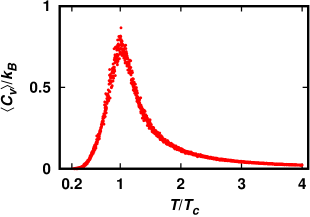
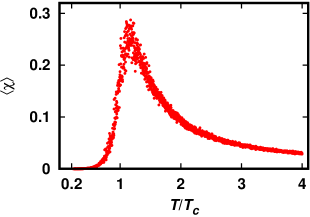
Phase transition is clearly observed from sharp changes in the diagrams of energy [Fig. 3.5] and magnetization [Fig. 3.5], also from the maximums of specific heat [Fig. 3] and zero-field magnetic susceptibility [Fig. 3], taking place at $T_{c}=2.5$. That the energy curve starts with its minimum value ($-J$ at $T\big{/}T_{c}=0.2$) is due to the fact that the initial configuration of the system has been chosen a minimum-energy microstate (all spins up). At $T=T_{c}$ energy undergoes a sharp raise, which, according to the thermodynamic relation $C_{v}=(\partial E\big{/}\partial T)_{N,V}$ gives rise to a maximum at this point. Maximums of the specific heats of solids, such as atomic clusters [33], are also clear manifestations of the solid-liquid phase transition: at the critical temperature, the energy of the system suddenly increases due to the fact that the binding energy of atoms is dominated by thermal fluctuations, increasing as well the kinetic energy of the atoms. The specific heat has been calculated using the energy fluctuation relation of the canonical ensemble

$$C_{v}=\frac{\langle(\Delta E)^{2}\rangle}{k_{B}T^{2}}=\frac{\langle E^{2}\rangle-\langle E\rangle^{2}}{k_{B}T^{2}}.$$

In contrast, the temperature dependence of $\langle M\rangle$, starting with its maximum, sharply decreases at the critical temperature and asymptotically approaches zero at high enough temperatures due to increase in the entropy of the system. Such a marked decrease is concurrent with the maximum in the temperature-dependent zero-field magnetic susceptibility of the system, calculated using the fluctuation-susceptibility relation

$$\chi=\frac{\langle(\Delta M)^{2}\rangle}{k_{B}T}=\frac{\langle M^{2}\rangle-\langle M\rangle^{2}}{k_{B}T}.$$

3.6 Output of code5.py: Visualizing the Ising lattice using XMakemol

Fig. 4 illustrates the output of code5.py for a $10\times 10$ lattice at $T=2.5$, visualized by XMakemol (version 5.16h) [34], which is a mouse-based software, written using LessTif [35] to render and manipulate atomic and chemical structures.

(a) sweep 1

(b) sweep 10

(c) sweep 850

Figure 4: A visualization of the outputs of code5.py simulating a 2D, $10\times 10$, square lattice of spin–1/2 particles at $T=2.5$ at three steps including (a) 1, (b) 10, and (c) 850. The red and blue balls respectively denote the up and down spins.

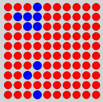
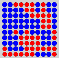
The input file required for creating such renders, namely spin.xyz, is generated by code5.py as an output file. To this end, we have added a simple snippet in our Python code, which stores the Cartesian components of each spin position (lattice point) at every MC step in the file spin.xyz, in that the up spins are defined as oxygen (O, red), and down spins as sodium (Na, blue) atoms, in the format readable to XMakemol. Fig. 5 also shows an output of code5.py for a $50\times 50$ lattice at $T=2.5$.

Figure 5: Output of code5.py simulating a 2D, $50\times 50$, square lattice of spin–1/2 particles at $T=2.5$.

4 Conclusions

A brief, comprehensive introduction to theory and simulation of the Ising model has been provided, which includes derivation of the Hamiltonian of the model, the computational details to numerically solve the 2D and 3D problems using the Monte Carlo method, the corresponding computer codes in both Python and Fortran, and a simulation trick to visualize the Ising lattice using XMakemol.

Appendix A Derivation of Eq. 1

The singlet ($\Psi_{s}$) and triplet ($\Psi_{t}$) wavefunctions associated with the system of two interacting electrons are

$$\Psi_{s}=\frac{1}{\sqrt{2}}\bigg{[}\phi_{1}(\mathrm{\bf{r}}_{1})\phi_{2}(\mathrm{\bf{r}}_{2})+\phi_{1}(\mathrm{\bf{r}}_{2})\phi_{2}(\mathrm{\bf{r}}_{1})\bigg{]}\chi_{s}$$

$$\Psi_{t}=\frac{1}{\sqrt{2}}\bigg{[}\phi_{1}(\mathrm{\bf{r}}_{1})\phi_{2}(\mathrm{\bf{r}}_{2})-\phi_{1}(\mathrm{\bf{r}}_{2})\phi_{2}(\mathrm{\bf{r}}_{1})\bigg{]}\chi_{t},$$

where $\phi_{1}(\mathrm{\bf{r}}_{1})$ is the position wavefunction of particle 1 at $\mathrm{\bf{r}}_{1}$, and $\chi_{s,t}$ are respectively the spin wavefunctions of the singlet and triplet states. The expectation values of the Hamiltonian $\hat{H}$ of the system in the singlet and triplet states are also respectively given by

$$E_{s}=\int\Psi_{s}^{*}\hat{H}\Psi_{s}d\mathrm{\bf{r}}_{1}d\mathrm{\bf{r}}_{2}$$

$$=\int\frac{1}{\sqrt{2}}\bigg{[}\phi_{1}^{*}(\mathrm{\bf{r}}_{1})\phi_{2}^{*}(\mathrm{\bf{r}}_{2})+\phi_{1}^{*}(\mathrm{\bf{r}}_{2})\phi_{2}^{*}(\mathrm{\bf{r}}_{1})\bigg{]}\hat{H}\frac{1}{\sqrt{2}}\bigg{[}\phi_{1}(\mathrm{\bf{r}}_{1})\phi_{2}(\mathrm{\bf{r}}_{2})+\phi_{1}(\mathrm{\bf{r}}_{2})\phi_{2}(\mathrm{\bf{r}}_{1})\bigg{]}d\mathrm{\bf{r}}_{1}d\mathrm{\bf{r}}_{2}$$

$$=\frac{1}{2}\int\bigg{[}\phi_{1}^{*}(\mathrm{\bf{r}}_{1})\phi_{2}^{*}(\mathrm{\bf{r}}_{2})\hat{H}\phi_{1}(\mathrm{\bf{r}}_{1})\phi_{2}(\mathrm{\bf{r}}_{2})\bigg{]}d\mathrm{\bf{r}}_{1}d\mathrm{\bf{r}}_{2}$$

$$+\frac{1}{2}\int\bigg{[}\phi_{1}^{*}(\mathrm{\bf{r}}_{1})\phi_{2}^{*}(\mathrm{\bf{r}}_{2})\hat{H}\phi_{1}(\mathrm{\bf{r}}_{2})\phi_{2}(\mathrm{\bf{r}}_{1})\bigg{]}d\mathrm{\bf{r}}_{1}d\mathrm{\bf{r}}_{2}$$

$$+\frac{1}{2}\int\bigg{[}\phi_{1}^{*}(\mathrm{\bf{r}}_{2})\phi_{2}^{*}(\mathrm{\bf{r}}_{1})\hat{H}\phi_{1}(\mathrm{\bf{r}}_{1})\phi_{2}(\mathrm{\bf{r}}_{2})\bigg{]}d\mathrm{\bf{r}}_{1}d\mathrm{\bf{r}}_{2}$$

$$+\frac{1}{2}\int\bigg{[}\phi_{1}^{*}(\mathrm{\bf{r}}_{2})\phi_{2}^{*}(\mathrm{\bf{r}}_{1})\hat{H}\phi_{1}(\mathrm{\bf{r}}_{2})\phi_{2}(\mathrm{\bf{r}}_{1})\bigg{]}d\mathrm{\bf{r}}_{1}d\mathrm{\bf{r}}_{2},$$

and

$$E_{t}=\int\Psi_{t}^{*}\hat{H}\Psi_{t}d\mathrm{\bf{r}}_{1}d\mathrm{\bf{r}}_{2}$$

$$=\int\frac{1}{\sqrt{2}}\bigg{[}\phi_{1}^{*}(\mathrm{\bf{r}}_{1})\phi_{2}^{*}(\mathrm{\bf{r}}_{2})-\phi_{1}^{*}(\mathrm{\bf{r}}_{2})\phi_{2}^{*}(\mathrm{\bf{r}}_{1})\bigg{]}\hat{H}\frac{1}{\sqrt{2}}\bigg{[}\phi_{1}(\mathrm{\bf{r}}_{1})\phi_{2}(\mathrm{\bf{r}}_{2})-\phi_{1}(\mathrm{\bf{r}}_{2})\phi_{2}(\mathrm{\bf{r}}_{1})\bigg{]}d\mathrm{\bf{r}}_{1}d\mathrm{\bf{r}}_{2}$$

$$=\frac{1}{2}\int\bigg{[}\phi_{1}^{*}(\mathrm{\bf{r}}_{1})\phi_{2}^{*}(\mathrm{\bf{r}}_{2})\hat{H}\phi_{1}(\mathrm{\bf{r}}_{1})\phi_{2}(\mathrm{\bf{r}}_{2})\bigg{]}d\mathrm{\bf{r}}_{1}d\mathrm{\bf{r}}_{2}$$

$$-\frac{1}{2}\int\bigg{[}\phi_{1}^{*}(\mathrm{\bf{r}}_{1})\phi_{2}^{*}(\mathrm{\bf{r}}_{2})\hat{H}\phi_{1}(\mathrm{\bf{r}}_{2})\phi_{2}(\mathrm{\bf{r}}_{1})\bigg{]}d\mathrm{\bf{r}}_{1}d\mathrm{\bf{r}}_{2}$$

$$-\frac{1}{2}\int\bigg{[}\phi_{1}^{*}(\mathrm{\bf{r}}_{2})\phi_{2}^{*}(\mathrm{\bf{r}}_{1})\hat{H}\phi_{1}(\mathrm{\bf{r}}_{1})\phi_{2}(\mathrm{\bf{r}}_{2})\bigg{]}d\mathrm{\bf{r}}_{1}d\mathrm{\bf{r}}_{2}$$

$$+\frac{1}{2}\int\bigg{[}\phi_{1}^{*}(\mathrm{\bf{r}}_{2})\phi_{2}^{*}(\mathrm{\bf{r}}_{1})\hat{H}\phi_{1}(\mathrm{\bf{r}}_{2})\phi_{2}(\mathrm{\bf{r}}_{1})\bigg{]}d\mathrm{\bf{r}}_{1}d\mathrm{\bf{r}}_{2}.$$

As a result, the energy difference between the two states is

$$E_{s}-E_{t}=\int\bigg{[}\phi_{1}^{*}(\mathrm{\bf{r}}_{1})\phi_{2}^{*}(\mathrm{\bf{r}}_{2})\hat{H}\phi_{1}(\mathrm{\bf{r}}_{2})\phi_{2}(\mathrm{\bf{r}}_{1})\bigg{]}d\mathrm{\bf{r}}_{1}d\mathrm{\bf{r}}_{2}+\int\bigg{[}\phi_{1}^{*}(\mathrm{\bf{r}}_{2})\phi_{2}^{*}(\mathrm{\bf{r}}_{1})\hat{H}\phi_{1}(\mathrm{\bf{r}}_{1})\phi_{2}(\mathrm{\bf{r}}_{2})\bigg{]}d\mathrm{\bf{r}}_{1}d\mathrm{\bf{r}}_{2}.$$ (11)

Assuming $\phi_{1}$ and $\phi_{2}$ to be real, and based on the fact that $\hat{H}$ is self-adjoint (then it can act on its left-hand side wavefunctions), Eq. 11 becomes

$$E_{s}-E_{t}=\int\bigg{[}\phi_{1}(\mathrm{\bf{r}}_{1})\phi_{2}(\mathrm{\bf{r}}_{2})\hat{H}\phi_{1}(\mathrm{\bf{r}}_{2})\phi_{2}(\mathrm{\bf{r}}_{1})\bigg{]}d\mathrm{\bf{r}}_{1}d\mathrm{\bf{r}}_{2}+\int\bigg{[}\phi_{1}(\mathrm{\bf{r}}_{1})\phi_{2}(\mathrm{\bf{r}}_{2})\hat{H}\phi_{1}(\mathrm{\bf{r}}_{2})\phi_{2}(\mathrm{\bf{r}}_{1})\bigg{]}d\mathrm{\bf{r}}_{1}d\mathrm{\bf{r}}_{2}$$

$$=2\int\bigg{[}\phi_{1}(\mathrm{\bf{r}}_{1})\phi_{2}(\mathrm{\bf{r}}_{2})\hat{H}\phi_{1}(\mathrm{\bf{r}}_{2})\phi_{2}(\mathrm{\bf{r}}_{1})\bigg{]}d\mathrm{\bf{r}}_{1}d\mathrm{\bf{r}}_{2}=2J$$ (12)

Appendix B Derivation of Eq. 2

From addition of two spins $\hat{s}_{1}$ and $\hat{s}_{2}$, we know that

$$\hat{S}=\hat{s}_{1}+\hat{s}_{2}\hskip 5.69054pt\Longrightarrow\hskip 5.69054pt\hat{S}^{2}=\hat{s}_{1}^{2}+\hat{s}_{2}^{2}+2\hat{s}_{1}.\hat{s}_{2}\hskip 5.69054pt\Longrightarrow\hskip 5.69054pt\hat{s}_{1}.\hat{s}_{2}=\frac{1}{2}\Big{[}\hat{S}^{2}-\hat{s}_{1}^{2}-\hat{s}_{2}^{2}\Big{]},$$

where $\hat{S}$ is the total spin operator of the two-electron system. Therefore,

$$|s_{1}-s_{2}|\leq S\leq|s_{1}+s_{2}|\hskip 5.69054pt\Longrightarrow\hskip 5.69054pt{S}= \left\{\begin{aligned} &1\hskip 14.22636pt\mathrm{Triplet}\\ &0\hskip 14.22636pt\mathrm{Singlet}\end{aligned}\right.$$

$$\hat{S}^{2}\ket{S,m_{S}}=S(S+1)\hbar^{2}\ket{S,m_{S}}\hskip 5.69054pt\Longrightarrow\hskip 5.69054ptS^{2}= \left\{\begin{aligned} &2\hskip 14.22636pt\mathrm{Triplet}\\ &0\hskip 14.22636pt\mathrm{Singlet}\end{aligned}\right.$$

$$\hat{s}_{1}^{2}\ket{s_{1},m_{s}}=s_{1}(s_{1}+1)\hbar^{2}\ket{s_{1},m_{s}}\hskip 5.69054pt\Longrightarrow\hskip 5.69054pts_{1}^{2}=s_{2}^{2}=\frac{3}{4}.$$

where characters without hats denote scalars. Further, because $\hat{S}^{2},\hat{s}_{1}^{2}$, and $\hat{s}_{2}^{2}$ are compatible observables, the eigenvalues of $\hat{s}_{1}.\hat{s}_{2}$, when acting on the common eigenstate of these three operators, are then

$$\frac{1}{2}\Big{(}S^{2}-s_{1}^{2}-s_{2}^{2}\Big{)}= \left\{\begin{aligned} &\frac{1}{2}\Big{(}2-\frac{3}{4}-\frac{3}{4}\Big{)}=\frac{1}{4}\hskip 22.19315pt\mathrm{Triplet}\\ &\frac{1}{2}\Big{(}0-\frac{3}{4}-\frac{3}{4}\Big{)}=-\frac{3}{4}\hskip 14.22636pt\mathrm{Singlet}\end{aligned}\right.$$ (13)

We indeed aim at constructing the Hamiltonian $\hat{H}$ in a way that (i) $\hat{H}$ when acting on $\Psi_{s}$ and $\Psi_{t}$ must respectively result in $E_{s}$ and $E_{t}$; (ii) $\hat{H}$ must be a function of the two spins $\hat{s}_{1}$ and $\hat{s}_{2}$, say $\hat{H}\propto\hat{s}_{1}.\hat{s}_{2}$; and (iii) Eq. 13 must hold. We particularly focus on the eigenvalues of $\hat{s}_{1}.\hat{s}_{2}$ (Eq. 13). For the triplet state, because the related eigenvalue is $1\big{/}4$, we then need one $(3\big{/}4)E_{t}$ to have a complete $E_{t}$ as the eigenvalue of the Hamiltonian. Likewise, for the singlet state, the related eigenvalue is $-3\big{/}4$, and we accordingly need one $(1\big{/}4)E_{s}$ with the minus sign for $\hat{s}_{1}.\hat{s}_{2}$ to have a complete $E_{s}$. Taking such crude considerations into account, one can construct an effective Hamiltonian in the form

$$\hat{H}=\frac{1}{4}E_{s}+\frac{3}{4}E_{t}-E_{s}\hat{s}_{1}.\hat{s}_{2}+E_{t}\hat{s}_{1}.\hat{s}_{2}=\frac{1}{4}\Big{(}E_{s}+3E_{t}\Big{)}-\Big{(}E_{s}-E_{t}\Big{)}\hat{s}_{1}.\hat{s}_{2},$$ (14)

which meets the requirements aforementioned. The precise value of $\big{(}E_{s}+3E_{t}\big{)}\big{/}4$ is indeed immaterial, and we can omit this by redefining the zero of energy; therefore, Eq. 14 turns into

$$\hat{H}=-2\sum_{i>j}J_{ij}\hat{s}_{i}.\hat{s}_{j},$$

where we have used Eq. A for $(E_{s}-E_{t})$ with $J\longrightarrow J_{ij}$.

References

- [1] M. Kardar, Statistical Physics of Particles, first ed., Cambridge University Press, 2007.
- [2] R.K. Pathria, P.D. Beale, Statistical Mechanics, third ed., Butterworth-Heinemann, Oxford, 2011.
- [3] S.J. Barnett, New Researches on Magnetization by Rotation and the Gyromagnetic Ratios of Ferromagnetic Substances, Proc. Am. Acad. Arts & Sci. 75 (1944) 109–129.
- [4] G.G. Scott, The Gyromagnetic Ratios of the Ferromagnetic Elements, Phys. Rev. 87 (1952) 697.
- [5] G.G. Scott, A Precise Mechanical Measurement of the Gyromagnetic Ratio of Iron, Phys. Rev. 82 (1951) 542.
- [6] R.G. Parr, W. Yang, Density-Functional Theory of Atoms and Molecules, Oxford University Press, New York, Oxford, 1989.
- [7] J. Kohanoff, Electronic Structure Calculations for Solids and Molecules: Theory and Computational Methods, first ed., Cambridge University Press, Cambridge, 2006.
- [8] D.J. Griffiths, Introduction to Quantum Mechanics, second ed., Pearson Prentice Hall, 2004.
- [9] W. Heisenberg, Zur Theorie des Ferromagnetismus, Z. Physik 49 (1928) 619–636.
- [10] W. Lenz, Beitrag zum Verständnis der magnetischen Erscheinungen in festen Körpern, Z. Physik 21 (1920) 613.
- [11] E. Ising, Beitrag zur Theorie des Ferromagnetismus, Z. Phys. 31 (1925) 253–258.
- [12] T. Matsubara, H. Matsuda, A Lattice Model of Liquid Helium, I, Prog. Theor. Phys. 16 (1956) 569–582.
- [13] D.D. Betts, M.H. Lee, Critical Properties of the XY Model, Phys. Rev. Lett. 20 (1968) 1507.
- [14] N. Metropolis, S. Ulam, The Monte Carlo Method, J. Am. Stat. Assoc. 44 (1949) 335–341.
- [15] N. Metropolis, A.W. Rosenbluth, M.N. Rosenbluth, A.H. Teller, E. Teller, Equations of state calculations by fast computing machines, J. Chem. Phys. 21 (1953) 1087–1092.
- [16] G.N. Lewis, A new principle of equilibrium, PNAS 11 (1925) 179–183.
- [17] D. Ter Haar, Foundations of Statistical Mechanics, Rev. Mod. Phys. 27 (1955) 289–338.
- [18] http://www.gimp.org/.
- [19] A.J. Beekman, L. Rademaker, J. van Wezel, arXiv:1909.01820v2.
- [20] A. Shekaari, M. Jafari, arXiv: 2103.16944v1.
- [21] A. Shekaari, M. Jafari, Unveiling the first post-graphene member of silicon nitrides: A novel 2D material, Comput. Mater. Sci. 180 (2020) 109693.
- [22] M. Jafari, A. Shekaari, N. Delavari, R. Jafari, Thermodynamic properties of TiC nanowire from first principles, J. Therm. Anal. Calorim. 138 (2019) 1167–1173.
- [23] A. Shekaari, M. Jafari, Electronic response of phagraphene membranes to excess charge carriers, Solid State Commun. 318 (2020) 113979.
- [24] A. Shekaari, M.R. Abolhassani, First-principles investigation of the thermodynamic properties of two-dimensional MoS2, Chin. J. Phys. 55 (2017) 105–114.
- [25] N.W. Ashcroft, N.D. Mermin, Solid State Physics, College ed., Harcourt, Inc., 1976.
- [26] A. Shekaari, M. Jafari, Effect of pairwise additivity on finite-temperature behavior of classical ideal gas, Physica A 497 (2018) 101–108.
- [27] A. Shekaari, M. Jafari, Structural dynamics of COVID-19 main protease, J. Mol. Struct. 1223 (2021) 129235.
- [28] A. Shekaari, M. Jafari, Non-equilibrium thermodynamic properties and internal dynamics of 32-residue beta amyloid fibrils, Physica A 557 (2020) 124873.
- [29] J. M. Haile, Molecular Dynamics Simulation: Elementary Methods, John Wiley & Sons, Inc., New York, 1992.
- [30] M. Lutz, Learning Python, fifth ed., O’Reilly Media, 2013.
- [31] S.J. Chapman, Fortran 95/2003 for Scientists and Engineers, third ed., McGraw-Hill Education, 2007.
- [32] www.gnuplot.info.
- [33] A. Shekaari, M. Jafari, Finite temperature properties and phase transition behavior of quasi-planar B36 nanocluster from first principles, Mater. Res. Express 6 (2019) 025014.
- [34] www.nongnu.org/xmakemol.
- [35] https://web.archive.org/web/20120723010742/http://lesstif.sourceforge.net/.