Quasi-stationary solutions of the surface quasi-geostrophic equation

Abstract

In the present study, we find that the surface quasi-geostrophic equation admits exact solutions, which evolve with time in quasi-stationary states. The solutions presented are available for any dissipation effect $\kappa(-\Delta)^{\alpha}$ ($\kappa>0$, $0\leq\alpha<1$), involved in the equation. When the equation is supercritical ($0\leq\alpha<\frac{1}{2}$), the problem on the existence of large global regular solutions remains open. This study, however, provides explicit sample solutions for the understanding of the uncertain problem.

1 Introduction

Consider the surface quasi-geostrophic equation

$$0=\partial_{t}\theta+\bm{u}\cdot\nabla\theta+\kappa(-\Delta)^{\alpha}\theta$$ (1)

for $0\leq\alpha<1$ and the dissipative parameter $\kappa>0$. Here $\theta$ is a scalar unknown representing potential temperature and $\bm{u}$ is the velocity expressed as

$$\bm{u}=(\partial_{y},-\partial_{x})(-\Delta)^{-\frac{1}{2}}\theta.$$

Equation (1) presents an interesting simple model that exhibits a number of nonlinear and dissipative characters of the 3D Navier-Stokes equations, and hence has been studied extensively. For the subcritical case $\frac{1}{2}<\alpha<1$, the existence of global solutions was obtained by Constantin and Wu [7]. When $\alpha=\frac{1}{2}$, equation (1) is critical, as it is comparable to the 3D Navier-Stokes equations with respect to a priori estimates in function spaces. However, the maximal principle, which is not applicable to the 3D Navier-Stokes equations, is available to (1). Thus global regular solutions remain existing (see Kiselev et al. [9]). For the supercritical case $0\leq\alpha<\frac{1}{2}$, the existence of local regular solutions and small global regular solutions have been obtained by Chae and Lee [1], Chen et al. [2], Wu [11] and Córdoda and Córododa [8] in a variety of function spaces. However, it is unknown for the existence of global regular solutions in the supercritical case. If the motion (1) is additionally driven by an external force, the existence of bifurcating stationary flows was studied by Chen and Price [5] and the author [3].

For the understanding of the dynamical behaviors of the solution to (1), we consider the equation to be $2\pi$-spatially periodic in the domain $\mathbb{T}^{2}=[0,2\pi)\times[0,2\pi)$, and simply present some exact solutions, which evolve in quasi-stationary states.

2 Exact solutions

The exact solution result is stated in the following.

Theorem 2.1.

Let $0\leq\alpha<1$ and $\kappa>0$. For any real constants $c_{1},...,c_{8}$, and integers $n,\,m$ with $nm\neq 0$ and $k$ so that

$$n^{2}+m^{2}=k^{2}\,\,\mbox{ whenever }\,\,(|c_{1}|+...+|c_{4}|)(|c_{1}|+...+|c_{4}|)\neq 0,$$ (2)

then (1) in $\mathbb{T}^{2}$ admits the following exact solution

$$\theta= e^{-\kappa(n^{2}+m^{2})^{\alpha}t}\Big{(}c_{1}\sin nx\sin my+c_{2}\cos nx\sin my+c_{3}\sin nx\cos my$$

$$\hskip 62.59605pt+c_{4}\cos nx\cos my\Big{)}$$

$$+e^{-\kappa|k|^{2\alpha}t}\Big{(}c_{5}\sin kx+c_{6}\sin ky+c_{7}\cos kx+c_{8}\cos ky\Big{)}.$$ (3)

Moreover, for any integers $n$ and $m$ with $|n|+|m|\neq 0$ and for any constants $a_{k}$ and $b_{k}$ so that $\sum_{k\in\mathbb{Z}}|k|(a_{k}^{2}+b_{k}^{2})<\infty$, then the function

$$\theta =\sum_{k\in\mathbb{Z}}e^{-\kappa(n^{2}k^{2}+m^{2}k^{2})^{\alpha}t}\Big{(}a_{k}\cos(knx+kmy)+b_{k}\sin(knx+kmy)\Big{)}$$ (4)

solves (1) in $\mathbb{T}^{2}$.

Proof.

The proof of (2.1) is straightforward.

For the validity with respect to $\theta$ given by (3), we see that

$$(-\Delta)^{-\frac{1}{2}}\theta=\lambda\theta\,\,\mbox{ for either }\,\,\lambda=\frac{1}{\sqrt{n^{2}+m^{2}}}\,\,\mbox{ or }\,\,\lambda=\frac{1}{|k|}.$$

This implies

$$\bm{u}\cdot\nabla\theta = \lambda(\partial_{y}\theta,-\partial_{x}\theta)\cdot\nabla\theta=0.$$

Rewrite (3) in the following form $\theta(t)=e^{-(-\Delta)^{\alpha}t}\theta(0),$ which solves the linear equation

$$\partial_{t}\theta+\kappa(-\Delta)^{\alpha}\theta=0$$ (5)

and hence solves (1).

For the validity with respect to $\theta$ given by (4), we see that

$$\bm{u}\cdot\nabla\theta= \Big{(}\partial_{y}(-\Delta)^{-\frac{1}{2}}\theta,-\partial_{x}(-\Delta)^{-\frac{1}{2}}\theta\Big{)}\cdot\nabla\theta$$

$$= \sum_{k,k^{\prime}\in\mathbb{Z}}e^{-\kappa(|k^{\prime}|^{2\alpha}+|k|^{2\alpha})(n^{2}+m^{2})^{\alpha}t}\frac{km(-a_{k}\varphi_{k}+b_{k}\phi_{k})nk^{\prime}(-a_{k^{\prime}}\varphi_{k^{\prime}}+b_{k^{\prime}}\phi_{k^{\prime}})}{\sqrt{n^{2}k^{2}+m^{2}k^{2}}}$$

$$- \sum_{k,k^{\prime}\in\mathbb{Z}}e^{-\kappa(|k^{\prime}|^{2\alpha}+|k|^{2\alpha})(n^{2}+m^{2})^{\alpha}t}\frac{kn(-a_{k}\varphi_{k}+b_{k}\phi_{k})mk^{\prime}(-a_{k^{\prime}}\varphi_{k^{\prime}}+b_{k^{\prime}}\phi_{k^{\prime}})}{\sqrt{n^{2}k^{2}+m^{2}k^{2}}}$$

$$= 0$$

for

$$\phi_{k}=\cos(knx+kmy)\,\,\mbox{ and }\,\,\varphi_{k}=\sin(knx+kmy).$$

Note that $\theta$ solves the linear equation (5) and hence solves (1).

The proof is complete. ∎

When $\kappa$ is as small as $0.001$ and $\alpha$ is close to the critical stage $\frac{1}{2}$, satisfactory numerical solutions of (1) via a spectral scheme were presented by Constantin et al. [6] by choosing respectively the following initial data

$$\sin x\sin y+\cos y,$$

$$-\cos 2x\cos y+\sin x\sin y,$$

$$\cos 2x\cos y+\sin x\sin y+\cos 2x\sin 3y.$$

As shown in [6], the flow patterns of the solutions initially from these data vary with the time $t$.

In the present study, however, the flow patterns of the exact solutions behave in a quasi-stationary manner. For example, we choose the solutions

$$\theta_{1} =e^{-5^{\alpha}\kappa t}(\sin 2x\sin y+\frac{1}{2}\cos 2x\cos y),$$ (6)

$$\theta_{2} =e^{-25^{\alpha}\kappa t}(\sin 4x\sin 3y+\frac{1}{2}\cos 4x\cos 3y+\sin 5y+\frac{1}{2}\sin 5x)$$ (7)

from (3), and the solution

$$\theta_{3} =e^{-2^{\alpha}\kappa t}\sin(x+y)+e^{-8^{\alpha}\kappa t}\sin(2x+2y)$$ (8)

from (4). They are displayed in Figure 1 for $\kappa=\alpha=0.001$.

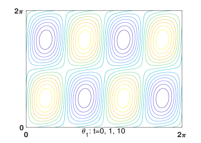
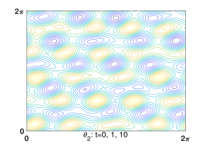
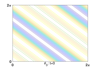
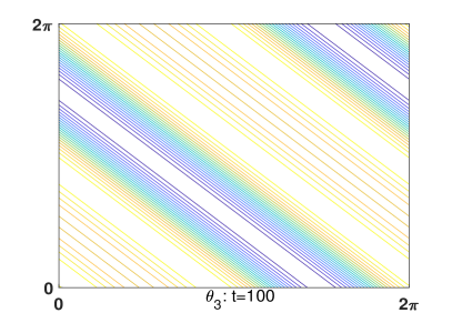
Figure 1: Exact solutions $\theta_{1}$, $\theta_{2}$ and $\theta_{3}$ for $\alpha=0.001$ and $\kappa=0.001$.

The solutions $\theta_{1}$ and $\theta_{2}$ as well as the solution (3) are quasi-stationary in the sense that their flow patterns remain unchanged (see Figure 1) as $t$ grows. This is due to the fact that the flow patterns defined by $\theta(t)=$constants are the same with those defined by $\theta(0)=$constants. Therefore, the flow patterns are not sensitive with the change of the parameters $\alpha$ and $\kappa$. The solution $\theta$ in (4) is a unidirectional flow moving along the parallel straight lines

$$nx+my={\rm constants}.$$

Figure 1 also shows that the solution $\theta_{3}$ as well as the solution (4) evolves in a quasi-stationary manner, as the flow patterns of $\theta_{3}$ for $t>0$ remain parallel to their initial form.

It should be noted that the exact solutions are for any $\kappa>0$ and $\alpha\geq 0$. In the numerical computation such as [6], it is difficult to keep the spectral scheme convergence when $\alpha$ is close to $0$. The vortex flow $e^{-\kappa(n^{2}+m^{2})^{\alpha}t}\sin nx\sin my$ is developed from the Taylor flow [10]. The present study is developed from the author’s recent investigation [4] on metastability of Kolmogorov flow.

Acknowledgment. This research was partially supported by NSFC of China (Grant No. 11571240).

References

• [1] D. Chae, J. Lee, Global well-posedness in the super-critical dissipative quasi-geostrophic equations, Commun. Math. Phys. 233 (2003), 297-311.
• [2] Q. Chen, C. Miao, Z. Zhang, A new Bernstein’s inequality and the 2D dissipative quasigeostrophic equation, Commun. Math. Phys. 271 (2007), 821-838.
• [3] Z.M. Chen, Bifurcating steady-state solutions of the dissipative quasi-geostrophic equation in Lagrangian formulation, Nonlinearity 29 (2016), 3132-3147.
• [4] Z.M. Chen, Enhanced and unenhanced dampings of Kolmogorov flow, preprint.
• [5] Z.M. Chen, W.G. Price, Stability and instability analyses of the dissipative quasi-geostrophic equation, Nonlinearity 21 (2008), 765-782.
• [6] P. Constantin, M.C. Lai, R. Sharma, Y.H. Tseng, J. Wu, New numerical results for the surface quasi-geostrophic equation, J. Sci. Comput. 50 (2012), 1-28.
• [7] P. Constantin, J. Wu, Behavior of solutions of 2D quasi-geostrophic equations, SIAM J. Math. Anal. 30 (1999), 937-948.
• [8] A. Córdoba, D. Córdoba, A maximum principle applied to quasi-geostrophic equations, Commun. Math. Phys. 249 (2004), 511-528.
• [9] A. Kiselev, F. Nazarov, A. Volberg, Global well-posedness for the critical 2d dissipative quasi-geostrophic equation, Invent. Math. 167 (2007), 445-453.
• [10] G.I. Taylor, On the decay of vortices in a viscous fluid, Philos. Mug. 46 (1923), 671-674.
• [11] J. Wu, Global solutions of the 2d dissipative quasi-geostrophic equation in Besov spaces, SIAM J. Math. Anal. 36 (2005), 1014-1030.