Enhanced and unenhanced dampings of Kolmogorov flow

Abstract

In the present study, Kolmogorov flow represents the stationary sinusoidal solution $(\sin y,0)$ to a two-dimensional spatially periodic Navier-Stokes system, driven by an external force. This system admits the additional non-stationary solution $(\sin y,0)+e^{-\nu t}(\sin y,0)$, which tends exponentially to the Kolmogorov flow at the minimum decay rate determined by the viscosity $\nu$. Enhanced damping or enhanced dissipation of the problem is obtained by presenting higher decay rate for the difference between a solution and the non-stationary basic solution. Moreover, for the understanding of the metastability problem in an explicit manner, a variety of exact solutions are presented to show enhanced and unenhanced dampings.

1 Introduction

Consider the two-dimensional periodically driven flow with viscosity $\nu>0$ governed by the Navier-Stokes equations

$$\partial_{t}\bm{u}+\bm{u}\cdot\nabla\bm{u}-\nu\Delta\bm{u}+\nabla p=\nu(a\sin y,0),\,\,\,\nabla\cdot\bm{u}=0$$ (1.1)

in the flat torus $\mathbb{T}_{\alpha}=[0,2\pi/\alpha)\times[0,2\pi)$ for $\alpha>0$ and $a\geq 0$. Therefore, the pressure $p$ and velocity $\bm{u}$ are subject to the spatially periodic condition with respect $2\pi/\alpha$ period in $x$ and $2\pi$ period in $y$. The vorticity formulation of (1.1) is expressed as

$$\partial_{t}\omega=-\bm{u}\cdot\nabla\omega+\nu\Delta\omega-\nu a\cos y=-J(\Delta^{-1}\omega,\omega)+\nu\Delta\omega-\nu a\cos y$$ (1.2)

with the Jacobian $J(\phi,\varphi)=\partial_{x}\phi\partial_{y}\varphi-\partial_{y}\phi\partial_{x}\varphi$. The velocity $\bm{u}$, vorticity $\omega$ and stream function $\psi$ of the flow are subject to the identities

$$\omega=-\Delta\psi\,\,\mbox{ and }\,\,\,\bm{u}=(\partial_{y}\psi,-\partial_{x}\psi).$$

This problem was introduced by Kolmogorov [1] in 1959 in a seminar, where he presented the stationary flow

$$\bm{u}=(a\sin y,0)\mbox{ or }\omega=-a\cos y,$$ (1.3)

which is known as Kolmogorov flow $(a=1)$, and encouraged turbulence study from the instability of the flow.

When $\alpha=1$, the linear stability of the Kolmogorov flow for all $\nu>0$ was given by Mishalkin and Sinai [12] and its nonlinear global stability was obtained by Marchioro [11]. When $0<\alpha<1$, Iudovich [9] showed the instability of Kolmogorov flow leading to the occurrence of secondary stationary flows. If the fluid domain is doubled to the size $[0,2\pi/\alpha)\times[0,4\pi)$, perturbations around the Kolmogorov flow give rise to Hopf bifurcation (see Chen and Price [4, 5]) into oscillatory flows. Nonlinear interaction arises from the coexistence of multiple secondary oscillatory flows from the Hopf bifurcation and develops into chaotic flows (see Chen and Price [6]). Turbulent Kolmogorov flow was also studied by Chandler and Kerswell [3].

In the present study, we are interested in stability problem of the Kolmogorov flow. Especially, for the unforced case $a=0$, the $L_{2}$ estimate of (1.2) in $\mathbb{T}_{\alpha}$ yields the damping of the enstrophy

$$\|\omega(t)\|_{L_{2}}\leq e^{-\nu t}\|\omega(0)\|_{L_{2}}\,\,\mbox{ for }\alpha\geq 1$$ (1.4)

at the minimum decay rate $\nu$. However, this damping may be enhanced for some class of initial data with respect to small $\nu$ or large Reynolds number $(Re=1/\nu)$. The enhanced damping problem was rased by Beck and Wayne [2]. They considered the equation

$$\partial_{t}\omega=\nu\Delta\omega-e^{-\nu t}\sin y\partial_{x}(1+\Delta^{-1})\psi,$$ (1.5)

which is linearized from the Navier-Stokes equation (1.2) with $a=0$ around its exact solution

$$\omega=-e^{-\nu t}\cos y.$$ (1.6)

When the non-local operator $\Delta^{-1}$ is not involved, they obtained the existence of constants $C$ and $M$ satisfying the estimate

$$\|\omega\|_{L_{2}}\leq Ce^{-M\sqrt{\nu}t}\|\omega(0)\|_{L_{2}},\,\,\,0<t\leq\frac{\tau}{\nu}$$ (1.7)

for given $\tau>0$, provided $\nu$ is small. The estimate (1.7) was recently obtained by Wei and Zhang [14] and Wei et al. [15] for the complete linear equation (1.5).

When $a=1$, Ibrahim et al. [8] considered the equation

$$\partial_{t}\omega=\nu\Delta\omega-a\sin y\partial_{x}(1+\Delta^{-1})\psi,$$ (1.8)

linearized around (1.3), and obtained the damping estimate (1.7).

The present study is actually motivated by the work of Lin and Xu [10], where they noticed that the linearized Navier-Stokes flow (1.5) is close to the linearized Euler flow

$$\partial_{t}\omega=-\sin y\partial_{x}(1+\Delta^{-1})\psi$$ (1.9)

for $t$ moderate and $\nu$ sufficiently small. Thus the low frequency modes leading to unenhanced damping can be controlled by the linearized Euler flow due to RAGE theorem [7]. They [10] considered the enhanced damping property of the linear equation (1.5) and the nonlinear equation (1.2) with $a=0$ as

$$\Big{\|}P_{\neq 0}\omega\Big{(}\frac{\tau}{\nu}\Big{)}\Big{\|}_{L_{2}}<\delta\|P_{\neq 0}\omega(0)\|_{L_{2}}$$

for given $\tau,\,\delta>0$, provided $\nu$ is small. Here $P_{\neq 0}$ is the projection operator

$$P_{\neq 0}\omega=\omega-\frac{\alpha}{2\pi}\int^{2\pi/\alpha}_{0}\omega dx.$$ (1.10)

Actually, equation (1.2) has the additional solution

$$\bm{u}=(a\sin y+e^{-\nu t}\sin y,\,0)\,\,\,\mbox{ or }\,\,\,\omega=-a\cos y-\cos ye^{-\nu t}.$$ (1.11)

Linearizing the Navier-Stokes equation (1.2) around (1.11), we have

$$\partial_{t}\omega=\nu\Delta\omega-a\sin y\partial_{x}(1+\Delta^{-1})\omega-e^{-\nu t}\sin y\partial_{x}(1+\Delta^{-1})\omega.$$ (1.12)

The present study is two fold. Firstly, we extend the analysis of Lin and Xu [10] to the forced Navier-Stokes equation (1.2). Secondly, to the understanding of the problem in a different direction, we present exact solutions showing the problem in an explicit manner.

The enhanced damping result reads as follows.

Theorem 1.1.

For any $\alpha>1$, $\tau>0$, $\delta>0$ and $a\in\{0,\,1\}$, then the following assertions hold true.

(i) Any solution $\omega$ to the linear equation (1.12) initiated from $\omega(0)\in L_{2}(\mathbb{T}_{\alpha})$ with $P_{\neq 0}\omega(0)=\omega(0)$ satisfies

$$\Big{\|}\omega\Big{(}\frac{\tau}{\nu}\Big{)}\Big{\|}_{L_{2}}<\delta\|\omega(0)\|_{L_{2}},$$

provided that $\nu>0$ is sufficiently small.

(ii)For any solution $\omega$ to the nonlinear equation (1.2) presented in the perturbed form

$$\omega=-a\cos y-\cos ye^{-\nu t}+\omega^{\prime},$$ (1.13)

then the perturbed flow $\omega^{\prime}$ satisfies

$$\Big{\|}P_{\neq 0}\omega^{\prime}(\frac{\tau}{\nu})\Big{\|}_{L_{2}}<\delta\Big{\|}P_{\neq 0}\omega^{\prime}(0)\Big{\|}_{L_{2}},$$

provided that $\omega(0)\in L_{2}(\mathbb{T}_{\alpha})$,

$$\|\omega^{\prime}(0)\|_{L_{2}}\leq\nu$$

and $\nu$ is sufficiently small.

When $a=1$, this result is on the stability of the Kolmogorov flow. Hence metastability rather than enhanced damping may be more suitable to address the present study.

When $a=0$, this result is comparable with that given by Lin and Xu [10] in the following.

Theorem 1.2.

([10, Theorem 1.2]) Consider the nonlinear NS equation (1.1) ( $a=0$ ) on $\mathbb{T}_{\alpha}$ with $\alpha\geq 1$. Denote $P_{\mathcal{K}}$ to be the projection of $L_{2}(\mathbb{T}_{\alpha})$ to the subspace of Kolmogorov flows $W_{\mathcal{K}}={\mathrm{s}pan}\{cosy,\sin y\}.$ Then,

(i) (Rectangular torus) Suppose $\alpha>1$. There exists $d>0$, such that for any $\tau>0$ and $\delta>0$, if $\nu$ is small enough, then for any solution $\omega^{\nu}(t)$ to (1.2) with initial data $\omega(0)\in L_{2}(\mathbb{T}_{\alpha})$ satisfying

$$\|(I-P_{\mathcal{K}})\omega^{\nu}(0)\|_{L_{2}}\leq d\nu,$$ (1.14)

we have

$$\Big{\|}P_{\neq 0}\omega^{\nu}\Big{(}\frac{\tau}{\nu}\Big{)}\Big{\|}_{L_{2}}<\delta\Big{\|}P_{\neq 0}\omega^{\nu}(0)\Big{\|}_{L_{2}}.$$ (1.15)

(ii) (Square torus) Suppose $\alpha=1$. There exist $d>0$, such that: for any $M>0$, $\tau>0$ and $\delta>0$, if $\nu$ is small enough , then for any solution $\omega^{\nu}(t)$ to (1.2) with initial data $\omega^{\nu}(0)\in L_{2}(\mathbb{T}_{\alpha})$ satisfying $\|(I-P_{\mathcal{K}})\omega^{\nu}(0)\|_{L_{2}}\leq d\nu$, either

$$\max_{0\leq t\leq\frac{\tau}{\nu}}\|P_{a}\omega^{\nu}(t)\|_{L_{2}}\geq M\|P_{\neq 0}\omega^{\nu}(0)\|_{L_{2}}$$ (1.16)

or

$$\inf_{0\leq t\leq\frac{\tau}{\nu}}\|(I-P_{a})P_{\neq 0}\omega^{\nu}(t)\|_{L_{2}}<\delta\|P_{\neq 0}\omega^{\nu}(0)\|_{L_{2}}$$ (1.17)

must hold true. Here $P_{a}$ is the orthogonal projection mapping $L_{2}$ onto the space span$\{\sin x,\cos x\}$.

Remark 1.1.

It should be noted that Theorem 1.2 or [10, Theorem 1.2] contradicts to the following fact:

For $\tau=M=1$, $\delta=e^{-\alpha^{2}-1}$ and any constant $d>0$, the function

$$\omega=d\nu\frac{\sqrt{\alpha}}{\sqrt{2}\pi}e^{-(\alpha^{2}+1)\nu t}\sin(\alpha x+y),\,\,\alpha\geq 1,$$ (1.18)

solves the Navier-Stokes equation (1.2) ($a=0$) in $\mathbb{T}_{\alpha}$ and has the following properties

$$\|(I-P_{\mathcal{K}})\omega(0)\|_{L_{2}} = \|\omega(0)\|_{L_{2}}=d\nu,\,\,\alpha\geq 1,$$

$$P_{\neq 0}\omega = \omega,\,\,\alpha\geq 1,$$

$$P_{a}\omega = 0,\,\,\alpha=1,$$

$$\|P_{\neq 0}\omega(t)\|_{L_{2}} \geq \delta\|P_{\neq 0}\omega(0)\|_{L_{2}},\,\,t\leq\frac{\tau}{\nu},\alpha>1,$$

$$\|((I-P_{a})P_{\neq 0}\omega(t)\|_{L_{2}} \geq \delta\|P_{\neq 0}\omega(0)\|_{L_{2}},\,\,t\leq\frac{\tau}{\nu},\alpha=1.$$

Therefore, the initial condition (1.14) holds ture, but none of the conclusion estimates (1.15)-(1.17) is valid, no matter how small the viscosity $\nu$ is.

Actually, Lin and Xu [10] considered estimating the perturbed flow $\omega^{\prime}(t)$ given by

$$\omega(t)=-\mathrm{e}^{-\nu t}\cos y+\omega^{\prime}(t)\mbox{ with }P_{\mathcal{K}}\omega^{\prime}(0)=0.$$

With the presence of the solution (1.18), a variety of exact solutions of the Navier-Stokes equation will be provided for showing their enhanced and unenhanced dampings.

Theorem 1.1 involves only the rectangular case $\alpha>1$, as the limit case $\alpha=1$ can be treated in a similar manner.

This paper is organized as follows. Theorem 1.1 is to be proved in Section 2. Exact solutions will be discussed in Section 3.

2 Proof of Theorem 1.1

The proof is developed from Lin and Xu [10] together with Constantin et al.[7]. The condition $\alpha>1$ is assumed throughout this section.

For convenience of notation, we always assume that $L_{2}(\mathbb{T}_{\alpha})$ denotes the $L_{2}$ space of all mean zero functions:

$$L_{2}(\mathbb{T}_{\alpha})=\Bigg{\{}\omega\,\,\Big{|}\,\,\int_{\mathbb{T}_{\alpha}}\omega dxdy=0,\|\omega\|_{L_{2}}^{2}=\int_{\mathbb{T}_{\alpha}}|\omega|^{2}dxdy<\infty\Bigg{\}}.$$

Recalling the operator $P_{\neq 0}$ from (1.10) , we define the $L_{2}$ subspaces $X=P_{\neq 0}L_{2}(\mathbb{T}_{\alpha})$, that is,

$$X=\Big{\{}\omega\in L_{2}(\mathbb{T}_{\alpha})\,\,|\,\,P_{\neq 0}\omega=\omega\Big{\}}.$$

It is convenience to use the equivalent $L_{2}$-norm

$$\|\omega\|_{X}=\|(1+\Delta^{-1})^{1/2}\omega\|_{L_{2}}$$ (2.1)

in the $L_{2}$ subspace $(1+\Delta^{-1})L_{2}(\mathbb{T}_{\alpha})$.

2.1 Preliminary estimates

As given by Lin and Xu [10], the enhanced damping lies on a modified RAGE theorem [7] with respect to the linearized Euler equation

$$\partial_{t}\omega=-(a+1)\sin y\partial_{x}(1+\Delta^{-1})\omega$$ (2.2)

in $X$, by avoiding unenhanced damping from low frequency eigenfunctions of the Laplacian operator $-\Delta$. We adopt the complete eigenvalues

$$\alpha^{2}\leq\lambda_{1}\leq\lambda_{2}\leq...$$

and the corresponding eigenfunctions $e_{1}$, $e_{2},...$ of the operator $-\Delta$ in $X$. Let $P_{N}$ be the $L_{2}$ projection mapping $X$ onto the subspace span$\{e_{1},...,e_{N}\}$.

Lemma 2.1.

([10, Lemma 2.3] and [7, Lemma 3.2]) Let $K\subset S\equiv\{\varphi\in X|\,\|\varphi\|_{L_{2}}=1\}$ be a compact set of $X$. For any $N,\kappa>0$, there exists $T_{c}(N,\kappa,K)$ such that for all $T\geq T_{c}$ and $\omega(0)/\|\omega(0)\|_{L_{2}}\in K$,

$$\frac{1}{T}\int^{T}_{0}\|P_{N}\omega(t)\|^{2}_{X}\leq\kappa\|\omega(0)\|^{2}_{X},$$ (2.3)

where $\omega(t)$ is the solution of the linearized Euler equation (2.2) initiated from $\omega(0)$.

Rewriting the Navier-Stokes equation (1.2) perturbed around the basic flow $-\cos y-e^{-\nu t}\cos y$, we have

$$\partial_{t}\omega= \nu\Delta\omega-a\sin y\partial_{x}(1+\Delta^{-1})\omega-\mathrm{e}^{-\nu t}\sin y\partial_{x}(1+\Delta^{-1})\omega$$

$$-\sigma J(\Delta^{-1}\omega,\omega),$$ (2.4)

with the constant $\sigma=0,\,1$. This equation is the linear one (1.12) for $\sigma=0$ and is the nonlinear perturbed form of (1.2) for $\sigma=1$.

The proof is essentially based on the fundamental $L_{2}$ estimate of the nonlinear Kolmogorov problem given by Iudovich [9, Eq. (2.14)],

$$\frac{d}{dt}\int_{\mathbb{T}_{\alpha}}\omega(t)(1+\Delta^{-1})\omega(t)dxdy=2\nu\int_{\mathbb{T}_{\alpha}}\Delta\omega(t)(1+\Delta^{-1})\omega(t)dxdy$$ (2.5)

or

$$\frac{d}{dt}\int_{\mathbb{T}_{\alpha}}\|\omega(t)\|^{2}_{X}+2\nu\|\nabla\omega(t)\|^{2}_{X}=0.$$ (2.6)

This estimate is simply obtained by taking the inner product of (2.4) with $(1+\Delta^{-1})\omega$ and using integration by parts.

The enhanced damping is to be confirmed when the solution to the previous equation is close to that of the linearized Euler equation (2.2).

Lemma 2.2.

For $\tau,\delta$ and $\nu$ in Theorem 1.1, Let $\omega^{\nu}$ be a solution of (2.4) with $\omega^{\nu}(0)\in L_{2}(\mathbb{T}_{\alpha})$. If the estimate

$$\|P_{\neq 0}\omega^{\nu}(t)-\omega^{0}(t)\|_{X}^{2}\leq\|P_{\neq 0}\omega^{\nu}(0)-\omega^{0}(0)\|_{X}^{2}+C_{1}\nu(1+t^{3})\|\nabla\omega^{0}(0)\|_{X}^{2}$$ (2.7)

holds true for a constant $C_{1}$ with respect to any solution $\omega^{0}$ of (2.2) initiated from

$$\omega^{0}(0)\in X^{1}\equiv\{\varphi\in X|\,\,\|\nabla\varphi\|_{X}<\infty\},$$

then

$$\Big{\|}P_{\neq 0}\omega^{\nu}\Big{(}\frac{\tau}{\nu}\Big{)}\Big{\|}_{L_{2}}<\delta\|P_{\neq 0}\omega^{\nu}(0)\|_{L_{2}}.$$ (2.8)

For the unforced case $a=0$, similar result has been presented in [10, pp. 1824-1825] originated from [7, Proof of Theorem 1.4]. Following [7], we adopt a compact set $K\subset S$ required by Lemma 2.1.

Proof.

For the given $\delta$ and $\tau>0$, we choose $N$ large enough so that

$$e^{-\lambda_{N}\tau}<\frac{\alpha^{2}}{\alpha^{2}-1}\delta^{2}.$$ (2.9)

In order to use Lemma 2.1, we adopt the compact set

$$K=\Big{\{}\phi\in X|\,\,\|\nabla\phi\|^{2}_{X}\leq\lambda_{N},\,\,\|\phi\|_{X}=1\Big{\}}.$$

Let $t_{1}=T_{c}(N,\frac{1}{10},K)$ from Lemma 2.1 and $C_{1}$ from (2.7). Choose a small viscosity $\nu_{0}$ so that

$$\nu_{0}C_{1}(1+t_{1}^{3})<\frac{1}{10\lambda_{N}}\,\,\,\mbox{ and }\,\,\,\nu_{0}<\frac{\tau}{3t_{1}}.$$ (2.10)

For any $0<\nu<\nu_{0}$, if

$$\lambda_{N}\|P_{\neq 0}\omega^{\nu}(t)\|^{2}_{X}\leq\|\nabla P_{\neq 0}\omega^{\nu}(t)\|^{2}_{X}$$

for all $t\in[0,\frac{\tau}{\nu}]$, it follows from (2.6) and (2.9) that

$$\Big{\|}P_{\neq 0}\omega^{\nu}\Big{(}\frac{\tau}{\nu}\Big{)}\Big{\|}^{2}_{X}\leq e^{-2\lambda_{N}\tau}\|P_{\neq 0}\omega^{\nu}(0)\|^{2}_{X}<\delta^{2}\|P_{\neq 0}\omega^{\nu}(0)\|^{2}_{L_{2}}$$ (2.11)

and we are done.

Otherwise, there exits $t_{0}\in[0,\frac{\tau}{\nu})$ being the first time in the interval such that

$$\|\nabla P_{\neq 0}\omega^{\nu}(t_{0})\|^{2}_{X}\leq\lambda_{N}\|P_{\neq 0}\omega^{\nu}(t_{0})\|^{2}_{X}.$$ (2.12)

Now we take the solution $\omega^{0}$ of (2.2) in the interval $[t_{0},t_{0}+t_{1}]$ so that $\omega^{0}(t_{0})=\omega_{0}\equiv P_{\neq 0}\omega^{\nu}(t_{0})$ . It follows from (2.7), (2.10) and (2.12) that

$$\|P_{\neq 0}\omega(t)-\omega^{0}(t)\|^{2}_{X} \leq\nu_{0}C_{1}(1+t_{1}^{3})\|\nabla\omega_{0}\|_{X}^{2}\leq\frac{1}{10}\|\omega_{0}\|_{X}^{2}.$$ (2.13)

Since $\omega_{0}/\|\omega_{0}\|_{X}\in K$, by the definition of $t_{1}$ and Lemma 2.1, we have

$$\frac{1}{t_{1}}\int^{t_{1}+t_{0}}_{t_{0}}\|P_{N}\omega^{0}(t)\|_{X}^{2}dt\leq\frac{1}{10}\|\omega_{0}\|_{X}^{2}.$$

By the conservation property (2.6) with $\nu=0$ for the linearized Euler equation, we have

$$\frac{1}{t_{1}} \int^{t_{1}+t_{0}}_{t_{0}}\|(I-P_{N})\omega^{0}(t)\|_{X}^{2}dt$$

$$=\|\omega_{0}\|^{2}_{X}-\frac{1}{t_{1}}\int^{t_{0}+t_{1}}_{t_{0}}\|P_{N}\omega^{0}(t)\|_{X}^{2}dt\geq\frac{9}{10}\|\omega_{0}\|_{X}^{2}.$$

This together with (2.13) implies

$$\frac{1}{t_{1}} \int^{t_{1}+t_{0}}_{t_{0}}\|(I-P_{N})P_{\neq 0}\omega^{\nu}(t)\|_{X}^{2}dt$$

$$\geq\frac{1}{t_{1}}\int^{t_{1}+t_{0}}_{t_{0}}\|(I-P_{N})\omega^{0}(t)\|_{X}^{2}dt-\frac{1}{t_{1}}\int^{t_{1}+t_{0}}_{t_{0}}\|P_{\neq 0}\omega^{\nu}(t)-\omega^{0}(t)\|_{X}^{2}dt$$

$$\geq\frac{4}{5}\|\omega_{0}\|_{X}^{2}.$$

Hence, we have

$$\int^{t_{0}+t_{1}}_{t_{0}}\|\nabla P_{\neq 0}\omega^{\nu}(t)\|^{2}_{X}dt \geq\lambda_{N}\int^{t_{0}+t_{1}}_{t_{0}}\|(I-P_{N})P_{\neq 0}\omega^{\nu}(t)\|^{2}_{X}$$

$$\geq\frac{4\lambda_{N}t_{1}}{5}\|\omega_{0}\|_{X}^{2}.$$

By (2.6), we have

$$\|P_{\neq 0}\omega^{\nu}(t_{0}+t_{1})\|^{2}_{X} =\|P_{\neq 0}\omega^{\nu}(t_{0})\|_{X}^{2}-2\nu\int^{t_{0}+t_{1}}_{t_{0}}\|\nabla P_{\neq 0}\omega^{\nu}(t)\|_{X}^{2}dt$$

$$\leq(1-\frac{8}{5}\lambda_{N}\nu t_{1})\|P_{\neq 0}\omega^{\nu}(t_{0})\|^{2}_{X}$$

$$\leq e^{-\frac{8}{5}\lambda_{N}\nu t_{1}}\|P_{\neq 0}\omega^{\nu}(t_{0})\|_{X}^{2}.$$ (2.14)

On the other hand, for any interval $[\tau_{1},\tau_{0}]$ such that

$$\|\nabla P_{\neq 0}\omega^{\nu}(t)\|^{2}_{X}\geq\lambda_{N}\|P_{\neq 0}\omega^{\nu}(t)\|^{2}_{X},\,\,\,\,t\in[\tau_{1},\tau_{0}],$$ (2.15)

we have by (2.6) that

$$\|P_{\neq 0}\omega^{\nu}(\tau_{1})\|^{2}_{X}\leq e^{-2\lambda_{N}\nu(\tau_{1}-\tau_{0})}\|P_{\neq 0}\omega^{\nu}(\tau_{0})\|_{X}^{2}.$$ (2.16)

Hence, the combination of all decay estimates from (2.14) and (2.16), and the use of $t_{1}<\frac{\tau}{3\nu}$ from (2.10) imply the existence of $t_{2}\in[\frac{2\tau}{3\nu},\frac{\tau}{\nu}]$ such that

$$\|P_{\neq 0}\omega^{\nu}(t_{2})\|^{2}_{X}\leq e^{-\frac{8}{5}\lambda_{N}\nu t_{2}}\|P_{\neq 0}\omega^{\nu}(0)\|_{X}^{2}\leq e^{-\lambda_{N}\tau}\|P_{\neq 0}\omega^{\nu}(0)\|_{X}^{2}.$$ (2.17)

Therefore, by (2.6) and (2.9), we have

$$\Big{\|}P_{\neq 0}\omega^{\nu}\Big{(}\frac{\tau}{\nu}\Big{)}\Big{\|}^{2}_{L_{2}} \leq\Big{\|}P_{\neq 0}\omega^{\nu}\Big{(}\frac{\tau}{\nu}\Big{)}\Big{\|}^{2}_{X}$$

$$\leq\|P_{\neq 0}\omega^{\nu}(t_{2})\|^{2}_{X}<\frac{\alpha^{2}\delta^{2}}{\alpha^{2}-1}\|P_{\neq 0}\omega^{\nu}(0)\|^{2}_{X}\leq\delta^{2}\|P_{\neq 0}\omega^{\nu}(0)\|_{L_{2}}^{2}.$$

This completes the proof of Lemma 2.2. ∎

2.2 Proof of Theorem 1.1

By Lemma 2.2, it suffices to prove the validity of (2.7) for the solutions $\omega^{\nu}$ of (2.4) and $\omega^{0}$ of (2.2) when $\omega^{\nu}(0)\in X$ and $\omega^{0}(0)\in X^{1}$.

Let $\omega=\omega^{\nu}_{1}-\omega^{0}$ with $\omega_{1}^{\nu}=P_{\neq 0}\omega^{\nu}$. Thus the difference $\omega$ is subject to the equation

$$\partial_{t}\omega= \nu\Delta\omega^{\nu}_{1}-a\sin y\partial_{x}(1+\Delta^{-1})\omega-\mathrm{e}^{-\nu t}\sin y\partial_{x}(1+\Delta^{-1})\omega$$

$$-(\mathrm{e}^{-\nu t}-1)\sin y\partial_{x}(1+\Delta^{-1})\omega^{0}+\sigma J(\Delta^{-1}\omega^{\nu},\omega^{\nu}).$$

Taking $L_{2}$ inner product of the previous equation with $(1+\Delta^{-1})\omega$ and integrating by parts, we have

$$\frac{1}{2}\frac{d}{dt} \|\omega(t)\|^{2}_{X}+\nu\|\nabla\omega_{1}^{\nu}(t)\|_{X}^{2}$$

$$= -\nu(\Delta\omega^{\nu}_{1},(1+\Delta^{-1})\omega^{0})-(\mathrm{e}^{-\nu t}-1)(\sin y\partial_{x}(1+\Delta^{-1})\omega^{0},(1+\Delta^{-1})\omega^{\nu}_{1})$$

$$+\sigma(J(\Delta^{-1}\omega^{\nu},\omega^{\nu}),(1+\Delta^{-1})\omega^{0}).$$ (2.18)

According to integration by parts, the first two linear terms on the right-hand side of (2.18) are bounded by

$$\nu\|\nabla\omega^{\nu}_{1}\|_{X} \|\nabla\omega^{0}\|_{X}+\nu t\|(1+\Delta^{-1})\omega^{0}\|_{L_{2}}\|\nabla(1+\Delta^{-1})\omega^{\nu}_{1}\|_{L_{2}}$$

$$\leq\nu\|\nabla\omega^{\nu}_{1}\|_{X}\|\nabla\omega^{0}\|_{X}+\nu t\|\omega^{0}\|_{X}\|\nabla\omega^{\nu}_{1}\|_{X}.$$ (2.19)

For the nonlinear problem, we estimate the last term on the right-hand side of (2.18) with $\sigma=1$. Adopt the orthogonal decomposition

$$\omega^{\nu}=\omega^{\nu}_{1}+\omega^{\nu}_{2}\,\,\mbox{ with }\,\,\omega_{2}^{\nu}=(I-P_{\neq 0})\omega^{\nu}.$$

By Hölder inequality and Sobolev imbedding, we have

$$-(J( \Delta^{-1}\omega^{\nu},\omega^{\nu}),(1+\Delta^{-1})\omega^{0})$$

$$= -\Big{(}J(\Delta^{-1}\omega^{\nu}_{2},\omega^{\nu}_{1})+J(\Delta^{-1}\omega^{\nu}_{1},\omega^{\nu}_{2})+J(\Delta^{-1}\omega^{\nu}_{1},\omega^{\nu}_{1}),(1+\Delta^{-1})\omega^{0}\Big{)}$$

$$\leq \Big{(}\|\Delta^{-1}\omega^{\nu}_{2}\|_{L_{\infty}}\|\nabla\omega^{\nu}_{1}\|_{L_{2}}+\|\nabla\Delta^{-1}\omega_{1}^{\nu}\|_{L_{\infty}}\|\omega^{\nu}_{2}\|_{L_{2}}+\|\Delta^{-1}\omega^{\nu}_{1}\|_{L_{\infty}}\|\nabla\omega_{1}\|_{L_{2}}\Big{)}$$

$$\cdot\|\nabla(1+\Delta^{-1})\omega^{0}\|_{L_{2}}$$

$$\leq C\|\nabla\omega_{1}^{\nu}\|_{X}(\|\omega^{\nu}_{2}\|_{L_{2}}+\|\omega^{\nu}_{1}\|_{L_{2}})\|\nabla\omega^{0}\|_{X}.$$ (2.20)

On the other hand, observing that the operator $1+\Delta^{-1}$ is positive on the space $(I-P_{\mathcal{K}})L_{2}(\mathbb{T}_{\alpha})$ and employing the $L_{2}$ estimate (2.5), we have

$$\|(I-P_{\mathcal{K}})\omega^{\nu}(t)\|_{L_{2}}^{2} \leq\frac{1}{1-\max\{\frac{1}{\alpha^{2}},\,\frac{1}{4}\}}(\omega^{\nu}(t),(1+\Delta^{-1})\omega^{\nu}(t))$$

$$\leq\frac{1}{1-\max\{\frac{1}{\alpha^{2}},\,\frac{1}{4}\}}(\omega^{\nu}(0),(1+\Delta^{-1})\omega^{\nu}(0))$$

$$\leq\frac{1}{1-\max\{\frac{1}{\alpha^{2}},\,\frac{1}{4}\}}\|\omega^{\nu}(0)\|_{L_{2}}^{2}.$$ (2.21)

Moreover, taking the inner product of (2.4) with $P_{\mathcal{K}}\omega^{\nu}$ and integrating by parts, we have

$$\frac{d}{dt} \|P_{\mathcal{K}}\omega^{\nu}\|^{2}_{L_{2}}$$

$$=-2\nu\|P_{\mathcal{K}}\omega^{\nu}\|^{2}_{L_{2}}-2(J(\Delta^{-1}(I-P_{\mathcal{K}})\omega^{\nu},(I-P_{\mathcal{K}})\omega^{\nu}),P_{\mathcal{K}}\omega^{\nu})$$

$$\leq-2\nu\|P_{\mathcal{K}}\omega^{\nu}\|^{2}_{L_{2}}+2\|\nabla\Delta^{-1}(I-P_{\mathcal{K}})\omega^{\nu}\|_{L_{2}}\|(I-P_{\mathcal{K}})\omega^{\nu}\|_{L_{2}}\|\nabla P_{\mathcal{K}}\omega^{\nu}\|_{L_{\infty}}$$

$$\leq-2\nu\|P_{\mathcal{K}}\omega^{\nu}\|^{2}_{L_{2}}+C\|(I-P_{\mathcal{K}})\omega^{\nu}\|_{L_{2}}^{2}\|P_{\mathcal{K}}\omega^{\nu}\|_{L_{2}}$$

$$\leq-\nu\|P_{\mathcal{K}}\omega^{\nu}\|^{2}_{L_{2}}+C\|\omega^{\nu}(0)\|_{L_{2}}^{4}.$$ (2.22)

Integrating (2.22) and combining the resultant equation with (2.21), we have

$$\|\omega^{\nu}(t)\|^{2}_{L_{2}} \leq\Big{(}1+\frac{1}{1-\max\{\frac{1}{\alpha^{2}},\,\frac{1}{4}\}}\Big{)}\|\omega^{\nu}(0)\|^{2}_{L_{2}}+C\int^{t}_{0}e^{-\nu(t-s)}\|\omega^{\nu}(0)\|_{L_{2}}^{4}ds$$

$$\leq C\Big{(}\|\omega^{\nu}(0)\|^{2}_{L_{2}}+\frac{1}{\nu}\|\omega^{\nu}(0)\|_{L_{2}}^{4}\Big{)}.$$ (2.23)

The combination of (2.18), (2.19) and (2.20) yields

$$\frac{d}{dt}\|\omega(t)\|^{2}_{X} \leq-2\nu\|\nabla\omega^{\nu}_{1}(t)\|_{X}^{2}+2\nu\|\nabla\omega^{\nu}_{1}(t)\|_{X}\|\nabla\omega^{0}(t)\|_{X}.$$ (2.24)

$$+2\nu t\|\omega^{0}(t)\|_{X}\|\nabla\omega^{\nu}_{1}(t)\|_{X}+C\sigma\|\nabla\omega^{\nu}_{1}(t)\|_{X}\|\omega^{\nu}(t)\|_{L_{2}}\|\nabla\omega^{0}(t)\|_{X}.$$

Therefore, by (2.23), the conservation of $\|\omega^{0}(t)\|_{X}^{2}$ from (2.6) with $\nu=0$, and the estimate [10, Lemma 2.3]

$$\|\nabla\omega^{0}(t)\|_{X}\leq C(1+t)\|\nabla\omega^{0}(0)\|_{X},$$

we have

$$\frac{d}{dt}\|\omega(t)\|^{2}_{X}$$

$$\leq-2\nu\|\nabla\omega^{\nu}_{1}(t)\|_{X}^{2}+C\nu\|\nabla\omega^{\nu}_{1}(t)\|_{X}((1+t)\|\nabla\omega^{0}(0)\|_{X}+t\|\omega^{0}(0)\|_{X})$$

$$+C\sigma\|\nabla\omega^{\nu}_{1}(t)\|_{X}(1+t)\|\nabla\omega^{0}(0)\|_{X}(\|\omega^{\nu}(0)\|^{2}_{L_{2}}+\frac{1}{\nu}\|\omega^{\nu}(0)\|_{L_{2}}^{4})^{1/2}.$$ (2.25)

If $\sigma=0$, the previous estimate implies (2.7). Otherwise, for $\sigma=1$, we use the assumption $\|\omega^{\nu}(0)\|_{L_{2}}\leq\nu$ and $\nu\leq 1$ to obtain from (2.25) that

$$\frac{d}{dt}\|\omega(t)\|^{2}_{X}\leq -2\nu\|\nabla\omega^{\nu}_{1}(t)\|_{X}^{2}+C\nu(1+t)\|\nabla\omega^{\nu}_{1}(t)\|_{X}\|\nabla\omega^{0}(0)\|_{X}$$

$$+C\nu t\|\nabla\omega^{\nu}_{1}(t)\|_{X}\|\omega^{0}(0)\|_{X}+C\nu\|\nabla\omega^{\nu}_{1}(t)\|_{X}(1+t)\|\nabla\omega^{0}(0)\|_{X}$$

$$\leq C\nu(1+t^{2})\|\nabla\omega^{0}(0)\|_{X}^{2}$$

with the constants $C$ independent of $\nu$. Hence, we obtain the validity of (2.7), after the integration of the previous equation.

The proof of Theorem 1.1 is complete.

3 Enhanced and unenhanced dampings of exact solutions

For the Navier-Stokes equation (1.2) with $\alpha>0$ and $a\in\{0,\,1\}$, we seek exact solutions $\omega$, satisfying the stationary Euler equation

$$J(\Delta^{-1}\omega,\omega)=0$$ (3.1)

at $t=0$, and in the form of

$$\omega=-a\cos y+e^{\nu\Delta t}\Big{(}\omega(0)+a\cos y\Big{)}.$$

3.1 Exact solutions of (1.2) with $a=1$

For any function

$$\phi=\sum_{n\geq 1}(a_{n}\cos ny+b_{n}\sin ny)\in L_{2}(\mathbb{T}_{\alpha}),$$

equation (1.2) has the exact solution

$$\omega =-\cos y+\mathrm{e}^{\nu\Delta t}\phi=-\cos y+\sum_{n\geq 1}e^{-n^{2}\nu t}(a_{n}\cos ny+b_{n}\sin ny)$$ (3.2)

due to the validity of (3.1) for $t\geq 0$.

The solution (1.2) is a unidirectional flow moving in horizontal lines $y=$ constants. Moreover, this solution is in the kernel of the projection operator $P_{\neq 0}$ and is absent in the metastability estimate in Theorem 1.1, due to the use of the RAGE theorem estimate in Lemma 2.1. However, equation (3.2) shows that the stability can be enhanced if $\omega$ involves high frequency modes only.

For non-unidirectional flow, we consider (1.2) in the extended domain

$$[0,2\pi/\alpha)\times[0,2\pi/\beta)\mbox{ with }\alpha^{2}+\beta^{2}=1\mbox{ and }1/\beta\in\mathbb{Z}.$$ (3.3)

Therefore, as in the perturbation form of (1.13), we have the exact solution

$$\omega= -a\cos y-\cos ye^{-\nu t}+e^{-\nu t}\Big{(}c_{1}\sin y+c_{2}\cos y+c_{3}\sin\alpha x\sin\beta y)$$

$$+e^{-\nu t}\Big{(}c_{4}\cos\alpha x\cos\beta y+c_{5}\sin\alpha x\cos\beta y+c_{6}\cos\alpha x\sin\beta y\Big{)}$$ (3.4)

for any constants $c_{i}$, since this function is subject to (3.1) for $t\geq 0$. This is a low frequency flow and the perturbed flow part decays at the minimum rate $\nu$. That is, Theorem 1.1 is no longer true if the fluid domain $\mathbb{T}_{\alpha}$ with $\alpha>1$ is replaced by the domain (3.3). For example, we choose a function from (3.4) as

$$\omega=-\cos y-\cos ye^{-\nu t}+e^{-\nu t}\Big{(}2\cos y+\sin\frac{\sqrt{3}}{2}x\sin\frac{1}{2}y\Big{)}$$ (3.5)

in the domain $[0,\frac{4\pi}{\sqrt{3}})\times[0,4\pi)$. This solution transforms initially from the four vortices state $\sin\frac{\sqrt{3}}{2}x\sin\frac{1}{2}y$ to the horizontal unidirectional flow $-\cos y$ (see Figure 1 at intermediate time states of the transition). This transition exhibits inverse cascade of two-dimensional fluid motion by enlarging two diagonal vortices, while other two vortices are compressed and then destroyed into pieces.

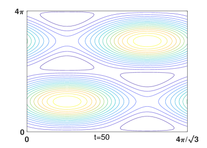
Figure 1: Vorticity contours for the exact solution (3.5) when $\nu=0.01$.

When $\alpha<1$, the Kolmogorov flow losses stability, but solutions (3.2) and (3.4) remain in its nonlinear stable manifold.

3.2 Exact solutions of (1.2) with $a=0$

For the case $a=0$, the basic stationary solution $-a\cos y$ becomes zero. We thus have more freedom to construct exact solutions.

Firstly, the unenhanced damping function (3.4) in the domain (3.3) solves (1.2) with $a=0$.

Secondly, to display solutions in $\mathbb{T}_{\alpha}$ with $\alpha>0$, we take any $n,\,m,\,i,\,j\in\mathbb{Z}$ and $a_{k},\,b_{k},\,c_{l}\in\mathbb{Re}$, and choose the following functions

$$\omega_{1} =\sum_{k\in\mathbb{Z}}e^{-\nu(n^{2}\alpha^{2}+m^{2})k^{2}t}(a_{k}\cos(kn\alpha x+kmy)+b_{k}\sin(kn\alpha x+kmy))$$ (3.6)

for $\omega_{1}(0)\in L_{2}(\mathbb{T}_{\alpha})$,

$$\omega_{2}= e^{-\nu(n^{2}\alpha^{2}+m^{2})t}\Big{(}c_{1}\sin n\alpha x\sin my+c_{2}\cos n\alpha x\sin my$$

$$\hskip 62.59605pt+c_{3}\sin n\alpha x\cos my+c_{4}\cos n\alpha x\cos my\Big{)},$$ (3.7)

$$\omega_{3}= \omega_{2}+e^{-\nu j^{2}t}(c_{5}\sin jy+c_{6}\cos jy),\,\,\mbox{ when }\alpha^{2}n^{2}+m^{2}=j^{2},$$ (3.8)

$$\omega_{4}= \omega_{2}+e^{-\nu i^{2}\alpha^{2}t}(c_{5}\sin i\alpha x+c_{6}\cos i\alpha x)$$

$$+e^{-\nu j^{2}t}(c_{7}\sin jy+c_{8}\cos jy),\,\,\mbox{ when }\,\alpha^{2}n^{2}+m^{2}=\alpha^{2}i^{2}=j^{2}.$$ (3.9)

It is readily seen that $\omega_{1},...,\omega_{4}$ solves (1.2). Indeed, to show $\omega_{1}$ satisfying (3.1) for $t\geq 0$, we see that

$$J (\Delta^{-1}\omega_{1},\omega_{1})$$

$$=\sum_{k,k^{\prime}\in\mathbb{Z}}e^{-\nu(k^{\prime 2}+k^{2})(\alpha^{2}n^{2}+m^{2})t}\frac{kn\alpha(-a_{k}\varphi_{k}+b_{k}\phi_{k})mk^{\prime}(-a_{k^{\prime}}\varphi_{k^{\prime}}+b_{k^{\prime}}\phi_{k^{\prime}})}{n^{2}\alpha^{2}k^{2}+m^{2}k^{2}}$$

$$-\sum_{k,k^{\prime}\in\mathbb{Z}}e^{-\nu(k^{\prime 2}+k^{2})(\alpha^{2}n^{2}+m^{2})t}\frac{km(-a_{k}\varphi_{k}+b_{k}\phi_{k})n\alpha k^{\prime}(-a_{k^{\prime}}\varphi_{k^{\prime}}+b_{k^{\prime}}\phi_{k^{\prime}})}{n^{2}\alpha^{2}k^{2}+m^{2}k^{2}}=0,$$

where we have used the condition $\omega_{1}(0)\in L_{2}(\mathbb{T}_{\alpha})$ to exclude mean zero functions and employed the notion

$$\phi_{k}=\cos(kn\alpha x+kmy)\,\,\mbox{ and }\,\,\varphi_{k}=\sin(kn\alpha x+kmy).$$

For the remaining functions $\omega_{l}$ with $l=2,\,3$ and $4$, we see that $\Delta^{-1}\omega_{l}$ is proportional to $\omega_{l}$ and thus (3.1) holds true for $t\geq 0$.

The solution $\omega_{1}$ is a unidirectional flow or a bar flow moving along the straight streamlines

$$n\alpha x+my=\mathrm{constants}.$$

For example, we take a function from (3.6) as

$$\omega= e^{-4(\alpha^{2}+1)\nu t}\sin(2\alpha x+2y)+e^{-16(\alpha^{2}+1)\nu t}\cos(4\alpha x+4y)$$

$$= e^{-\sqrt{\nu}t}\sin(2\alpha x+2y)+e^{-4\sqrt{\nu}t}\cos(4\alpha x+4y)$$ (3.10)

in $\mathbb{T}_{\alpha}$ for $\alpha=\sqrt{6}/2$. Here $\nu=0.01$ for showing the enhanced damping $e^{-\sqrt{\nu}t}$. Vortex contours of the solution (3.10) are displayed in Figure 2.

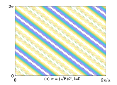
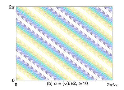
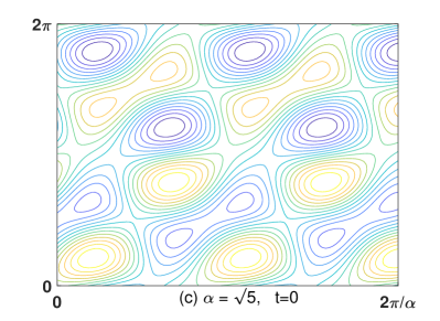
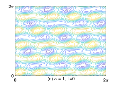
Figure 2: Vorticity contours of solutions (3.10) in (a)-(b), (3.11) in (c) and (3.12) in (d) for $\nu=0.01$.

For non-unidirectional flows, we choose a function from (3.8) in $\mathbb{T}_{\alpha}$ with $\alpha=\sqrt{5}$ in the following from

$$\omega =e^{-\frac{9}{10}\sqrt{\nu}t}(\sin(\sqrt{5}x)\sin(2y)+0.3\cos(\sqrt{5}x)\cos(2y)+0.4\sin(3y)),$$ (3.11)

where $\nu=0.01$. From (3.9), we take the following function

$$\omega=e^{-\frac{5}{2}\sqrt{\nu}t}\Big{(} 0.4\sin(4x)\sin(3y)+0.5\cos(4x)\cos(3y)$$

$$+\sin(5y)+0.3\sin(5x)\Big{)},\,\,\,\nu=0.01,$$ (3.12)

in the domain $\mathbb{T}_{\alpha}$ with $\alpha=1$.

The enhanced damping flows (3.11) and (3.12) are displayed in Figure 2 (c)-(d). The solutions (3.7)-(3.9) or (3.11)-(3.12) are in the form of

$$\omega(t)=e^{-(a^{2}n^{2}+m^{2})\nu t}\omega(0),$$ (3.13)

which decays with $t$. However, the vorticity contours of $\omega(t)$ on the horizontal planes $z=$constants are the same with those of $\omega(0)$ on the horizontal planes $z=e^{(\alpha^{2}n^{2}+m^{2})\nu t}$cosntants. Therefore, in Figure 2 (c)-(d), we only provide vorticity contours at the initial state $t=0$, as the flow patterns remain quasi-stationary when $t$ grows. On the other hand, when $\nu$ is sufficiently small and $t$ is moderate, the exact solutions evolve in a quasi-stationary manner and are close to their initial states, which solve the stationary Euler equation. Solutions (3.6)-(3.9) also exhibit quasi-stationary states such as bar states (unidirectional flows), dipole states and quadrupole states discussed by Yin et al. [16] in a turbulence decaying problem.

It should be noted that the solution $e^{-(\alpha^{2}n^{2}+m^{2})\nu t}\sin(\alpha nx)\sin(my)$ is known as Taylor flow given by Taylor [13].

Remark 3.1.

If the fluid domain is the horizontal channel $\mathbb{Re}\times[0,2\pi]$ and the fluid motion is additionally driven by the up moving boundary in the following sense

$$\bm{u}|_{y=2\pi}=(2\pi,0),\,\,\,\bm{u}|_{y=0}=(0,0),$$

the Navier-Stokes system (1.1) refers to a forced Couette flow problem and has the exact unidirectional solution

$$\bm{u}=\Big{(}y+a\sin y+\sum_{n\geq 1}e^{-\nu n^{2}t}a_{n}\sin ny,\,0\Big{)}$$

for any coefficients $a_{n}$ so that $\sum_{n\geq 1}a_{n}^{2}<\infty$.

References

- [1] V.I. Arnold, L.D. Meshalkin, A.N. Kolmogorov’s seminar on selected problems of analysis (1958-1959), Russ. Math. Surv. 15 (1960), 247-250.
- [2] M. Beck, C.E. Wayne, Metastability and rapid convergence to quasi-stationary bar states for the two-dimensional Navier-Stokes equations, Proc. R. Soc. Edinburgh A 143 (2013), 905-927.
- [3] G.J. Chandler, R.R. Kerswell, Invariant recurrent solutions embedded in a turbulent two-dimensional Kolmogorov flow, J. Fluid Mech. 722 (2013), 554-595.
- [4] Z.M. Chen, W.G. Price, Remarks on the time dependent periodic Navier-Stokes flows on a two-dimensional torus, Commun. Math. Phys. 207 (1999), 81 - 106.
- [5] Z.M. Chen, W.G. Price, Supercritical regimes of liquid-metal fluid motions in electromagnetic fields: wall-bounded flows, Proc. R. Soc. Lond. A 458 (2002), 2735-2757.
- [6] Z.M. Chen, W.G. Price, Onset of chaotic Kolmogorov flows resulting from interacting oscillatory modes, Commun. Math. Phys. 256 (2005), 737-766.
- [7] P. Constantin, A. Kiselev, L. Ryzhik, A. Zlatos, Diffusion and mixing in fluid flow, Annals Math. 168 (2008), 643-674.
- [8] S. Ibrahim, Y. Maekawa, N. Masmoudi, On pseudospectral bound for non-selfadjoint operators and Its application to stability of Kolmogorov flows, Annals of PDE 5 (2019), 1-84.
- [9] V.I. Iudovich, Example of the generation of a secondary stationary or periodic flow when there is loss of stability of the laminar flow of a viscous incompressible fluid, J. Appl. Math. Mech. 29 (1965), 527-544.
- [10] Z. Lin, M. Xu, Metastability of Kolmogorov Flows and Inviscid Damping of Shear Flows, Arch. Rational Mech. Anal. 231 (2019), 1811-1852.
- [11] C. Marchioro, An example of absence of turbulence for any Reynolds number, Commun. Math. Phys. 105(1986), 99-106.
- [12] L.D. Meshalkin, Ya.G. Sinai, Investigation of the stability of a stationary solution of a system of equations for the plane movement of an incompressible viscous fluid, J. Math. Mech. 19 (1961), 1700-1705
- [13] G.I. Taylor, On the decay of vortices in a viscous fluid, Philos. Mug. 46 (1923), 671-674.
- [14] D. Wei, Z. Zhang, Enhanced dissipation for the Kolmogorov flow via the hypocoercivity method, Sci. China Math. 62 (2019), 1219-1232.
- [15] D. Wei, Z. Zhang, W. Zhao, Linear inviscid damping and enhanced dissipation for the Kolmogorov flow, Adv. Math. 362, 106963 (2020).
- [16] Z. Yin, D.C. Montgomery, H.J.H. Clercx, Alternative statistical-mechanical descriptions of decaying two-dimensional turbulence in terms of “patches” and “points”, Phys. Fluids 15, 1937 (2003).