Poisson-Boltzmann formulary: Second edition

Abstract

The Poisson-Boltzmann (PB) equation provides a mean-field theory of electrolyte solutions at interfaces and in confinement, with numerous applications ranging from colloid science to nanofluidics. This formulary gathers important formulas for the PB description of a $Z$:$Z$ electrolyte solution inside slit and cylindrical channels. Different approximated solutions (thin electrical double layers, no co-ion, Debye-Hückel, and homogeneous/parabolic potential limits) and their range of validity are discussed, together with the full solution for the slit channel. In addition, different boundary conditions are presented, the limits of the PB framework are briefly discussed, and Python scripts to solve the PB equation numerically are provided.

I Introduction

When an electrolyte solution meets a solid surface, several mechanisms can generate a surface charge, together with an opposite charge carried by ions in the liquid (typical mechanisms include dissociation of surface groups and specific adsorption of charged species) [1, 2, 3]. In the vicinity of a charged wall, ions reorganize to form a diffuse charged layer, the electrical double layer (EDL), which screens the surface electric field over the so-called Debye length denoted $\lambda_{\text{D}}$, see Fig. 1(a-b). The EDL plays a key role in many aspects of soft condensed matter, as it controls the stability and dynamics of charged objects in solution [1, 2, 3]. In particular, the EDL is at the origin of the so-called electrokinetic effects, where gradients and fluxes of different types (hydrodynamic, electrical, chemical, thermal) are coupled in the presence of charged interfaces [4]. Such electrokinetic effects are central to the very active field of nanofluidics [5, 6, 7, 8].

The ion distribution and electric potential profile in the EDL can be computed by combining the Poisson equation for electrostatics and the Boltzmann distribution of the ions into the so-called Poisson-Boltzmann (PB) equation, under certain assumptions [9, 10]:

• the Poisson equation is written assuming that the solvent has a local, homogeneous and isotropic dielectric permittivity;

• the Boltzmann distribution of the ions is written assuming that the energy of the ions results only from their Coulomb interactions with the other ions and the wall, described at a mean-field level.

Educational presentations of the PB theory can be found in books [1, 2, 3], book chapters [9, 10], and articles [4], discussing in particular applications to nanofluidics [5, 6, 7, 8].

In contrast, this formulary simply gathers important formulas for the description of the EDL with the PB equation, focusing on a $Z$:$Z$ electrolyte solution inside slit and cylindrical channels, see Fig. 1(c) and Fig. 1(d), respectively. After introducing the notations (Sec. II) and important characteristic lengths (Sec. III), the formulary describes the cases of a slit channel (Sec. IV) and of a cylindrical channel (Sec. V). For both geometries, different approximated solutions are discussed: the thin EDL limit, where $\lambda_{\text{D}}$ is small as compared to the channel size; the no co-ion limit, where the EDLs overlap and the surface charge is large enough that co-ions are excluded; the Debye-Hückel limit at low surface charge, where the PB equation can be linearized. The range of validity of these approximations is then discussed; for the slit channel only, the general solution is presented. Finally the limits of the PB framework are briefly discussed in Sec. VII.

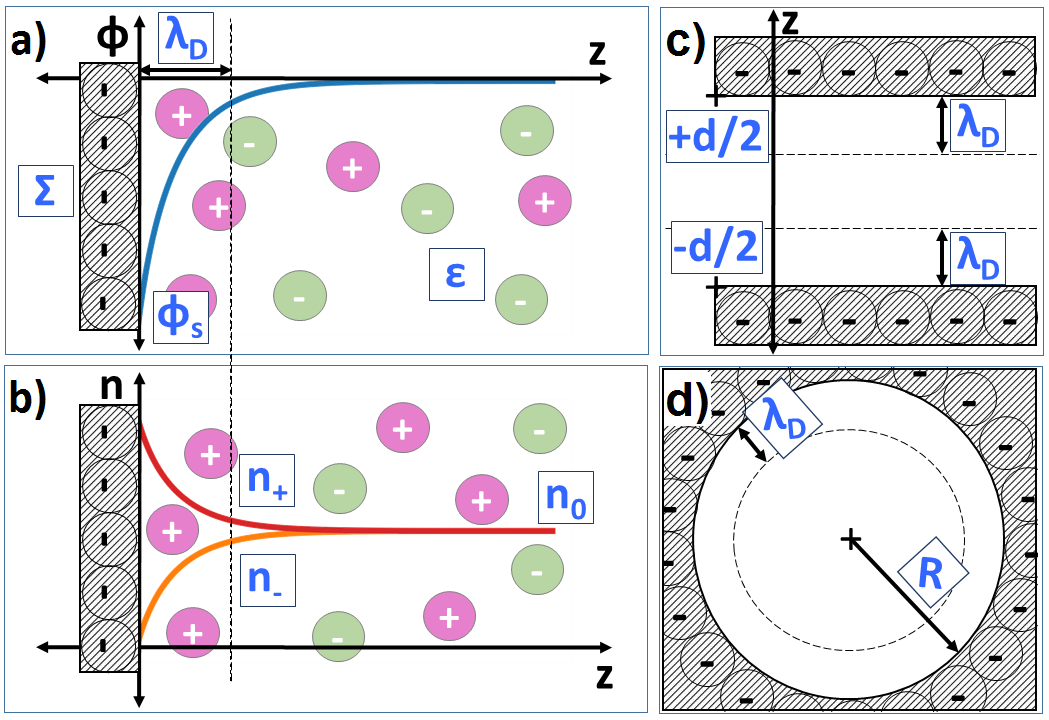
Figure 1: a-b) Local picture of the electrical double layer at a charged wall ($z$ is the distance from the wall, $\Sigma$ the surface charge density, $\varepsilon$ the solvent dielectric permittivity, and $\lambda_{\text{D}}$ the Debye length): a) Profile of reduced electric potential $\phi$, with $\phi_{\text{s}}$ the value at the wall; b) Profiles of cation $n_{+}$ and anion $n_{-}$ densities, with $n_{0}$ the bulk value. c) Schematics of the slit channel. d) Schematics of the cylindrical channel.

II Notations

• solvent dielectric permittivity $\varepsilon$

• inverse thermal energy $\beta=1/(k_{\text{B}}T)$, with $k_{\text{B}}$ the Boltzmann constant and $T$ the temperature

• absolute ionic charge $q=Ze$, with $e$ the elementary charge and $Z$ the ion valence

• ion densities $n_{\pm}$

• charge density $\rho_{\text{e}}$

• salt concentration $n_{0}=n_{+}=n_{-}$ in the bulk/reservoirs

• surface charge density $\Sigma$

• electrostatic potential $V$

• reduced potential $\phi=\beta qV$

• their value at the wall $V_{\text{s}}$ and $\phi_{\text{s}}$

• auxiliary reduced potential $\psi=-\text{sgn}(\Sigma)\times\phi$

• Bjerrum length $\ell_{\text{B}}$

• Debye length $\lambda_{\text{D}}$

• Gouy-Chapman length $\ell_{\text{GC}}$

• $\chi=\lambda_{\text{D}}/\ell_{\text{GC}}$

• Dukhin length $\ell_{\text{Du}}$

III Characteristic lengths

Solvent permittivity $\varepsilon$: Bjerrum length $\ell_{\text{B}}$ –

The Bjerrum length is the distance at which the electrostatic interaction energy between two ions is equal to the thermal energy $k_{\text{B}}T$.

$$\ell_{\text{B}}=\frac{\beta q^{2}}{4\pi\varepsilon}\quad\Leftrightarrow\quad\varepsilon=\frac{\beta q^{2}}{4\pi\ell_{\text{B}}}$$ (1)

For a monovalent salt in water at room temperature, $\ell_{\text{B}}\sim 0.7$ nm.

Bulk salt concentration $n_{0}$: Debye length $\lambda_{\text{D}}$ –

The Debye length is the range of the exponential screening of the electric field in an electrolyte.

$$\lambda_{\text{D}}=\frac{1}{\sqrt{8\pi\ell_{\text{B}}n_{0}}}\quad\Leftrightarrow\quad n_{0}=\frac{1}{8\pi\ell_{\text{B}}\lambda_{\text{D}}^{2}}$$ (2)

For a monovalent salt in water at room temperature, $\lambda_{\text{D}}\sim 0.3\,\text{nm}/\sqrt{n_{0}\text{(mol/L)}}$.

Surface charge density $\Sigma$: Gouy-Chapman length $\ell_{\text{GC}}$ –

The Gouy-Chapman length is the distance at which the electrostatic interaction energy between an ion and a charged surface is comparable to the thermal energy $k_{\text{B}}T$.

$$\ell_{\text{GC}}=\frac{q}{2\pi\ell_{\text{B}}|\Sigma|}\quad\Leftrightarrow\quad\Sigma=\text{sgn}(\Sigma)\frac{q}{2\pi\ell_{\text{B}}\ell_{\text{GC}}}$$ (3)

For monovalent ions in water at room temperature, $\ell_{\text{GC}}\sim 36\,\text{nm}/|\Sigma|\mathrm{(mC/m^{2})}$.

In the following, it will appear that many quantities can be expressed as a function of the ratio $\chi=\lambda_{\text{D}}/\ell_{\text{GC}}$, which is proportional to the absolute value of the surface charge, and inversely proportional to the square root of the bulk salt concentration:

$$\chi=\frac{\lambda_{\text{D}}}{\ell_{\text{GC}}}=2\pi\ell_{\text{B}}\lambda_{\text{D}}\frac{|\Sigma|}{q}=\frac{|\Sigma|/q}{\sqrt{n_{0}}}\sqrt{\frac{\pi\ell_{\text{B}}}{2}}$$

Surface ions vs bulk ions: Dukhin length $\ell_{\text{Du}}$ –

The Dukhin length is the channel scale at which the number of salt ions in bulk compares to the number of counter-ions at the surfaces [6].

$$\ell_{\text{Du}}=\frac{\absolutevalue{\Sigma}/q}{n_{0}}$$ (4)

IV Slit channel

This section gathers the equations describing a $Z$:$Z$ electrolyte solution confined between two planar parallel walls at a distance $d$, see Fig. 1(c).

IV.1 Thin EDLs: one wall with salt

When the distance $d$ between the surfaces is much larger than the thickness of the EDLs, one can solve the PB equation for a single charged wall, and superimpose the potentials of the two walls to obtain the full potential in the channel. The limits of validity of this approximation will be quantified in section IV.4.

Accordingly, this section gathers formulas for the description of a $Z$:$Z$ electrolyte solution in contact with a single planar wall, where $z\geq 0$ is the distance from the wall, see Fig. 1(a) and (b).

IV.1.1 PB equation: derivation

Poisson equation:

$$-\varepsilon\dfrac{\mathrm{d}^{2}V}{\mathrm{d}z^{2}}=\rho_{\text{e}}(z)=q\{n_{+}(z)-n_{-}(z)\}$$

Boltzmann distribution:

$$n_{\pm}(z)=n_{0}\,\exp{\mp\beta qV(z)}$$

Poisson-Boltzmann equation

$$\frac{\mathrm{d}^{2}\phi}{\mathrm{d}z^{2}}=\frac{1}{\lambda_{\text{D}}^{2}}\sinh\{\phi(z)\}$$ (5)

IV.1.2 PB equation: solution

Multiplying both sides of Eq. (5) by $\mathrm{d}\phi/\mathrm{d}z$ and integrating between $z=\infty$ and $z$; imposing that $\mathrm{d}\phi/\mathrm{d}z|_{z=\infty}=\phi(\infty)=0$:

$$\frac{1}{2}\left(\frac{\mathrm{d}\phi}{\mathrm{d}z}\right)^{2}=\frac{1}{\lambda_{\text{D}}^{2}}\left\{\cosh(\phi)-1\right\}$$ (6)

Noting that $\cosh(\phi)-1=2\sinh^{2}(\phi/2)$, and that $\phi$ and $\mathrm{d}\phi/\mathrm{d}z$ are of opposite sign:

$$\frac{\mathrm{d}\phi}{\mathrm{d}z}=-\frac{2}{\lambda_{\text{D}}}\sinh\left(\frac{\phi}{2}\right)$$ (7)

Noting that $\sinh(\phi/2)=2\sinh(\phi/4)\cosh(\phi/4)=2\tanh(\phi/4)\cosh^{2}(\phi/4)$, and integrating like a physicist:

$$\int_{\phi_{\text{s}}}^{\phi}\frac{\mathrm{d}(\phi/4)}{\tanh(\phi/4)\cosh^{2}(\phi/4)}=-\int_{0}^{z}\frac{\mathrm{d}z}{\lambda_{\text{D}}}\\ \quad\Rightarrow\quad\ln\left|\tanh\left(\frac{\phi}{4}\right)\right|-\ln\left|\tanh\left(\frac{\phi_{\text{s}}}{4}\right)\right|=-\frac{z}{\lambda_{\text{D}}}$$

Noting that $\phi$ and $\phi_{\text{s}}$ have the same sign:

$$\tanh\left(\frac{\phi}{4}\right)=\tanh\left(\frac{\phi_{\text{s}}}{4}\right)e^{-\frac{z}{\lambda_{\text{D}}}}$$

Noting that $\text{atanh}(x)=\frac{1}{2}\ln\left(\frac{1+x}{1-x}\right)$, and defining

$$\gamma=\tanh\left(\frac{\phi_{\text{s}}}{4}\right)$$ (8)

one finally gets:

$$\phi(z)=4\,\text{atanh}\left\{\gamma e^{-\frac{z}{\lambda_{\text{D}}}}\right\}=2\ln\left(\frac{1+\gamma e^{-\frac{z}{\lambda_{\text{D}}}}}{1-\gamma e^{-\frac{z}{\lambda_{\text{D}}}}}\right)$$ (9)

IV.1.3 Surface charge and surface potential

Electrostatics at the interface:

$$-\left.\frac{\mathrm{d}V}{\mathrm{d}z}\right|_{z=0}=\frac{\Sigma}{\varepsilon}\\ \quad\Rightarrow\quad\left.\frac{\mathrm{d}\phi}{\mathrm{d}z}\right|_{z=0}=-4\pi\ell_{\text{B}}\,\frac{\Sigma}{q}=-\frac{2\,\text{sgn}(\Sigma)}{\ell_{\text{GC}}}$$ (10)

Note that Eq. (10) also follows from the global electroneutrality of the system:

$$\int_{0}^{\infty}\rho_{\text{e}}\differential z=-\int_{0}^{\infty}\varepsilon\frac{\differential^{2}V}{\differential z^{2}}\differential z=\varepsilon\left.\frac{\mathrm{d}V}{\mathrm{d}z}\right|_{z=0}=-\Sigma$$

Using Eq. (7), one obtains Grahame equation relating $\phi_{\text{s}}$ and $\Sigma$:

$$\sinh\left(\frac{\phi_{\text{s}}}{2}\right)=2\pi\ell_{\text{B}}\lambda_{\text{D}}\,\frac{\Sigma}{q}=\text{sgn}(\Sigma)\chi$$ (11)

so that $\phi_{\text{s}}$ can be expressed as:

$$\phi_{\text{s}}=2\,\text{sgn}(\Sigma)\,\text{asinh}\left(\chi\right)\\ =2\,\text{sgn}(\Sigma)\ln\left\{\chi+\sqrt{1+\chi^{2}}\right\}$$ (12)

One can also express $\gamma=\tanh(\phi_{\text{s}}/4)$ as a function of $\Sigma$, or equivalently as a function of $\chi$:

$$\gamma=\frac{\text{sgn}(\Sigma)}{\chi}\left\{-1+\sqrt{1+\chi^{2}}\right\}$$ (13)

IV.1.4 A few integrals

Electrostatic energy $\mathcal{E}$

$$\mathcal{E}=\frac{\varepsilon}{2}\int_{0}^{\infty}\left(\frac{\mathrm{d}V}{\mathrm{d}z}\right)^{2}\,\mathrm{d}z=\frac{1}{8\pi\ell_{\text{B}}\beta}\int_{0}^{\infty}\left(\frac{\mathrm{d}\phi}{\mathrm{d}z}\right)^{2}\,\mathrm{d}z\\ =\frac{1}{2\pi\ell_{\text{B}}\lambda_{\text{D}}\beta}\left\{-1+\sqrt{1+\chi^{2}}\right\}=\frac{|\gamma|}{2\pi\ell_{\text{B}}\ell_{\text{GC}}\beta}$$ (14)

Ionic densities

• Total density excess

  Using Eq. (6),

  $$n_{+}+n_{-}-2n_{0}=2n_{0}\left\{\cosh(\phi)-1\right\}=\frac{1}{8\pi\ell_{\text{B}}}\left(\frac{\mathrm{d}\phi}{\mathrm{d}z}\right)^{2}$$

  Therefore,

  $$\int_{0}^{\infty}\left(n_{+}+n_{-}-2n_{0}\right)\,\mathrm{d}z=\beta\mathcal{E}$$ (15)

• Density difference

  Electroneutrality imposes that:

  $$\int_{0}^{\infty}\rho_{\text{e}}(z)\,\mathrm{d}z=-\Sigma$$

  Remembering that $\rho_{\text{e}}=q(n_{+}-n_{-})$, one gets:

  $$\int_{0}^{\infty}(n_{+}-n_{-})\,\mathrm{d}z=-\frac{\Sigma}{q}=-\frac{\text{sgn}(\Sigma)}{2\pi\ell_{\text{B}}\ell_{\text{GC}}}$$ (16)

More integrals

$$\mathcal{F}=\int_{0}^{\infty}\left(\phi_{\text{s}}-\phi\right)\left(\frac{\mathrm{d}\phi}{\mathrm{d}z}\right)^{2}\,\mathrm{d}z\\ =\frac{8\,\text{sgn}(\Sigma)}{\lambda_{\text{D}}}\left\{\chi-\text{asinh}(\chi)\right\}$$ (17)

$$\mathcal{G}=\int_{0}^{\infty}z\left(\frac{\mathrm{d}\phi}{\mathrm{d}z}\right)^{2}\,\mathrm{d}z=-4\ln\left(1-\gamma^{2}\right)$$ (18)

IV.1.5 Thickness of the EDL

The thickness of the EDL is often identified with the Debye length $\lambda_{\text{D}}$. However, at high $|\Sigma|$, the charge of the EDL is concentrated in a region much thinner than $\lambda_{\text{D}}$. The characteristic thickness of the charged region can be defined as:

$$\lambda=\frac{\int_{0}^{\infty}z\,\rho_{\text{e}}(z)\,\mathrm{d}z}{\int_{0}^{\infty}\rho_{\text{e}}(z)\,\mathrm{d}z}=\frac{\varepsilon V_{\text{s}}}{\Sigma}=\frac{V_{\text{s}}}{-\left.\frac{\mathrm{d}V}{\mathrm{d}z}\right|_{z=0}}=\frac{\phi_{\text{s}}}{-\left.\frac{\mathrm{d}\phi}{\mathrm{d}z}\right|_{z=0}}$$

Using Eq. (10) and Eq. (12), one gets:

$$\lambda=\lambda_{\text{D}}\frac{\text{asinh}\left(\chi\right)}{\chi}=\ell_{\text{GC}}\,\text{asinh}\left(\chi\right)$$ (19)

The characteristic scale for the variation of the electric field can also be written, following Weisbuch and Guéron [11]:

$$\lambda^{\prime}=\frac{\left.-\frac{\mathrm{d}\phi}{\mathrm{d}z}\right|_{z=0}}{\left.\frac{\mathrm{d}^{2}\phi}{\mathrm{d}z^{2}}\right|_{z=0}}=\frac{\lambda_{\text{D}}}{\sqrt{1+\chi^{2}}}$$ (20)

The limits at low and high surface charge of these characteristic scales are reported in section IV.1.6 (Table 1).

IV.1.6 Low and high surface charge limits

Critical surface charge

When the surface charge $|\Sigma|$ is low enough that the reduced potential $|\phi|$ is much lower than 1 everywhere, and therefore when $|\phi_{\text{s}}|=\max(|\phi|)\ll 1$, the PB equation can be linearized; this is the Debye-Hückel (DH) regime.

Using Grahame equation, Eq. (11), it appears that this regime is found when $\chi=\lambda_{\text{D}}/\ell_{\text{GC}}\ll 1$. The related critical surface charge for which $\lambda_{\text{D}}=\ell_{\text{GC}}$ writes:

$$|\Sigma|_{\text{c}}=\frac{q}{2\pi\ell_{\text{B}}\lambda_{\text{D}}}=\sqrt{\frac{8\varepsilon n_{0}}{\beta}}$$ (21)

For instance, for a monovalent salt in water at room temperature:

$$|\Sigma|_{\text{c}}\sim\frac{36\,\text{mC/m}^{2}}{\lambda_{\text{D}}\text{(nm)}}\sim 120\,\text{mC/m}^{2}\sqrt{n_{0}\text{(mol/L)}}$$ (22)

In practice, the linearized equation only provides a fair description for $|\Sigma|\lesssim 0.2|\Sigma|_{\text{c}}=24\,\text{mC/m}^{2}\sqrt{n_{0}\text{(mol/L)}}$. Thus, except at very high salt concentration, the DH regime is only found for very low surface charge.

Debye-Hückel regime

When $\chi=\lambda_{\text{D}}/\ell_{\text{GC}}\ll 1$, the PB equation can be linearized and its solutions simplified:

• the PB equation becomes: $\dfrac{\mathrm{d}^{2}\phi}{\mathrm{d}z^{2}}=\dfrac{1}{\lambda_{\text{D}}^{2}}\phi$

• the potential becomes: $\phi(z)=\phi_{\text{s}}\,\text{e}^{-z/\lambda_{\text{D}}}$

• $\gamma$ becomes $\phi_{\text{s}}/4$

• the Grahame relation becomes: $V_{\text{s}}/\lambda_{\text{D}}=\Sigma/\varepsilon$

Some limits at low and high surface charge

The limits of $\phi_{\text{s}}$, $\gamma$, $\mathcal{E}$, $\lambda$, $\lambda^{\prime}$, $\mathcal{F}$ and $\mathcal{G}$ at low and high surface charge are reported in Table 1.

Quantity	$\chi=\lambda_{\text{D}}/\ell_{\text{GC}}\ll 1$	$\chi=\lambda_{\text{D}}/\ell_{\text{GC}}\gg 1$
$\phi_{\text{s}}$	$\text{sgn}(\Sigma)2\chi=\beta q\dfrac{\Sigma\lambda_{\text{D}}}{\varepsilon}$	$2\,\text{sgn}(\Sigma)\ln\left(2\chi\right)$
$\gamma$	$\text{sgn}(\Sigma)\dfrac{\chi}{2}=\beta q\dfrac{\Sigma\lambda_{\text{D}}}{4\varepsilon}$	$\text{sgn}(\Sigma)$
$\mathcal{E}$	$\dfrac{\chi^{2}}{4\pi\beta\ell_{\text{B}}\lambda_{\text{D}}}=\dfrac{\Sigma^{2}\lambda_{\text{D}}}{4\varepsilon}$	$\dfrac{\chi}{2\pi\beta\ell_{\text{B}}\lambda_{\text{D}}}=\dfrac{|\Sigma|}{\beta q}$
$\lambda$	$\lambda_{\text{D}}$	$\ell_{\text{GC}}\ln\left(2\chi\right)$
$\lambda^{\prime}$	$\lambda_{\text{D}}$	$\ell_{\text{GC}}$
$\mathcal{F}$	$\dfrac{4\,\text{sgn}(\Sigma)\chi^{3}}{3\lambda_{\text{D}}}$	$\dfrac{8\,\text{sgn}(\Sigma)\chi}{\lambda_{\text{D}}}$
$\mathcal{G}$	$\chi^{2}$	$4\ln\left(\dfrac{\chi}{2}\right)$

Table 1: One wall with salt: limits of $\phi_{\text{s}}$, $\gamma$, $\mathcal{E}$, $\lambda$, $\lambda^{\prime}$, $\mathcal{F}$ and $\mathcal{G}$ for $\chi=\lambda_{\text{D}}/\ell_{\text{GC}}\ll 1$ (low surface charge, DH regime) and for $\chi=\lambda_{\text{D}}/\ell_{\text{GC}}\gg 1$ (high surface charge regime).

IV.2 Thick EDLs, high surface charge: two walls, no co-ion

When the EDLs overlap and for large enough surface charges (these conditions will be quantified in section IV.4), co-ions are excluded from the channel and the PB equation can be solved with counter-ions only.

IV.2.1 PB equation: derivation

Let’s consider counter-ions with density $n(z)$ confined between two parallel walls located at $z=-d/2$ and $z=d/2$, baring the same surface charge density $\Sigma$.

In order to make the equations describing a negative surface charge (with positive counter-ions) or a positive surface charge (with negative counter-ions) identical, one can define an auxiliary reduced potential $\psi$, which will always be negative:

$$\psi=-\text{sgn}(\Sigma)\times\phi=-\text{sgn}(\Sigma)\times\beta qV.$$ (23)

The potential in the middle of the channel is arbitrarily fixed to zero: $\psi_{\text{m}}=\psi(z=0)=0$ (this condition will be relaxed in section IV.3.4). Denoting $n_{\text{m}}$ the counter-ion density at $z=0$, and introducing a new characteristic length $K^{-1}$,

$$K^{-1}=\frac{1}{\sqrt{2\pi\ell_{\text{B}}n_{\text{m}}}}\quad\Leftrightarrow\quad n_{\text{m}}=\frac{K^{2}}{2\pi\ell_{\text{B}}},$$ (24)

one can derive the PB equation.

Poisson equation:

$$qn(z)=-\dfrac{\varepsilon}{\beta q}\dfrac{\mathrm{d}^{2}\psi}{\mathrm{d}z^{2}}$$

Boltzmann distribution:

$$n(z)=n_{\text{m}}\,\mathrm{e}^{-\psi(z)}$$

Poisson-Boltzmann equation:

$$\dfrac{\mathrm{d}^{2}\psi}{\mathrm{d}z^{2}}=-2K^{2}\,\mathrm{e}^{-\psi(z)}$$ (25)

IV.2.2 PB equation: solution

$$\psi(z)=\ln\left\{\cos^{2}(Kz)\right\}$$ (26)

$$\dfrac{\mathrm{d}\psi}{\mathrm{d}z}=-2K\tan(Kz)$$ (27)

$$n(z)=\dfrac{n_{\text{m}}}{\cos^{2}(Kz)}=\dfrac{K^{2}}{2\pi\ell_{\text{B}}\cos^{2}(Kz)}$$ (28)

IV.2.3 Surface charge and surface potential

To fully determine the potential and ion density profiles, one needs to express $K$ as a function of the surface charge.

Electrostatics at the interface (or equivalently, global electroneutrality):

$$\left.\frac{\mathrm{d}V}{\mathrm{d}z}\right|_{z=d/2}=\frac{\Sigma}{\varepsilon}\quad\Rightarrow\quad\left.\frac{\mathrm{d}\psi}{\mathrm{d}z}\right|_{z=d/2}=-\frac{2}{\ell_{\text{GC}}}$$ (29)

Using Eq. (27), one obtains:

$$Kd\,\tan\left(\frac{Kd}{2}\right)=\frac{d}{\ell_{\text{GC}}}.$$ (30)

Equation (30) only provides an implicit expression for $K$, but a very accurate explicit approximation (error below $0.07$ %) can be written:

$$\frac{Kd}{2}\approx\frac{\pi}{2}\sqrt{\frac{x(x+5)}{x^{2}+9x+5\pi^{2}/2}},$$ (31)

with $x=d/\ell_{\text{GC}}$.

Simpler approximate expressions can also be derived in the low and high surface charge limits, see Sec. IV.2.5.

IV.2.4 A few integrals

Electrostatic energy $\mathcal{E}$

$$\mathcal{E}=\frac{\varepsilon}{2}\int_{-d/2}^{d/2}\left(\frac{\mathrm{d}V}{\mathrm{d}z}\right)^{2}\,\mathrm{d}z\\ =\frac{2}{\pi d\ell_{\text{B}}\beta}\frac{Kd}{2}\left[\tan\left(\frac{Kd}{2}\right)-\frac{Kd}{2}\right]$$ (32)

An approximate expression as a function of $x=d/\ell_{\text{GC}}$ (error below $1$ %) can be written:

$$\mathcal{E}\approx\frac{1}{\pi d\ell_{\text{B}}\beta}\times\frac{x^{2}}{6-\sqrt{x}/5+x}.$$ (33)

Ionic density

$$\int_{-d/2}^{d/2}n(z)\,\mathrm{d}z=\frac{2|\Sigma|}{q}=\frac{1}{\pi\ell_{\text{B}}\ell_{\text{GC}}}$$ (34)

IV.2.5 Low and high surface charge limits

Low surface charge

When $\Sigma$ is small enough that $d/\ell_{\text{GC}}\ll 1$, Eq. (30) simplifies:

$$Kd\approx\sqrt{2d/\ell_{\text{GC}}},$$ (35)

which is accurate within 1 % up to $d/\ell_{\text{GC}}\approx 0.12$.

Note that when $d/\ell_{\text{GC}}\ll 1$, $Kd\ll 1$, so that $\psi\approx 0$ and the ion density is approximately homogeneous in the channel:

$$n\approx\dfrac{K^{2}}{2\pi\ell_{\text{B}}}=\dfrac{1}{\pi d\ell_{\text{B}}\ell_{\text{GC}}}.$$ (36)

This is commonly called the ideal gas regime. In practice, the ion density varies by less than 10 % over the channel thickness as long as $d/\ell_{\text{GC}}<0.2$.

High surface charge

When $\Sigma$ is large enough that $d/\ell_{\text{GC}}\gg 1$, Eq. (30) simplifies:

$$Kd\approx\frac{\pi}{1+\frac{2\ell_{\text{GC}}}{d}},$$ (37)

which is accurate within 1 % down to $d/\ell_{\text{GC}}\approx 7$.

Eventually, when $d/\ell_{\text{GC}}\rightarrow\infty$, $Kd\rightarrow\pi$, and the potential and ion density profiles reach a limit, sometimes referred to as the “Gouy-Chapman limit”:

$$\psi(z)=\ln\left\{\cos^{2}(\pi z/d)\right\}$$ (38)

$$n(z)=\dfrac{\pi}{2d^{2}\ell_{\text{B}}\cos^{2}(\pi z/d)}$$ (39)

IV.3 General case: two walls with salt

IV.3.1 Exact solution

In the general case of an aqueous electrolyte confined between two symmetrical parallel walls located at $z=-d/2$ and $z=d/2$, the potential profile can be written in terms of the Jacobi elliptic functions cd, sn, cn and dn.

As for the no co-ion regime (see Sec. IV.2), one can define an auxiliary reduced potential $\psi$, which is always negative:

$$\psi=-\text{sgn}(\Sigma)\times\phi=-\text{sgn}(\Sigma)\times\beta qV.$$ (40)

The auxiliary potential writes:

$$\psi(y)=2\ln\left\{\sqrt{m}\ \text{cd}\left(\frac{yr_{1}}{2\sqrt{m}},m^{2}\right)\right\},$$ (41)

where $y=z/d\in[-0.5;0.5]$ is the reduced position, $r_{1}=d/\lambda_{\text{D}}$, and $m=\exp(\psi_{\text{m}})$ with $\psi_{\text{m}}$ the potential in the middle of the slab. The parameter $m$ is the solution of:

$$r_{2}=\frac{1-m^{2}}{2\sqrt{m}}\times\frac{\text{sn}\left(\frac{r_{1}}{4\sqrt{m}},m^{2}\right)}{\text{cn}\left(\frac{r_{1}}{4\sqrt{m}},m^{2}\right)\text{dn}\left(\frac{r_{1}}{4\sqrt{m}},m^{2}\right)},$$ (42)

where $r_{2}=\lambda_{\text{D}}/\ell_{\text{GC}}$. For a given $r_{1}$, $m$ lies in the interval $]m_{0},1[$, where $m_{0}$ the solution of $4\sqrt{m}K(m^{2})=r_{1}$ (with $K(x)$ the complete elliptic integral of the first kind).

The PB equation can also be solved numerically (a Python script to that aim is provided in the appendix, A.1), and different approximate solutions for the auxiliary reduced potential $\psi$ expressed as a function of the reduced position $y=z/d$ can be written depending on $r_{1}$ and $r_{2}$, discussed in the following.

IV.3.2 Debye-Hückel limit

When the reduced potential $|\psi|$ is small everywhere (this condition will be quantified in section IV.4), the PB equation can be linearized (DH regime, already encountered when considering only one wall in Sec. IV.1).

With the conditions:

$$\left.\frac{\mathrm{d}\psi}{\mathrm{d}z}\right|_{z=0}=0\quad\text{and}\quad\left.\frac{\mathrm{d}\psi}{\mathrm{d}z}\right|_{z=d/2}=-\frac{2}{\ell_{\text{GC}}},$$

the solution to the linearized PB equation, $\frac{\mathrm{d}^{2}\psi}{\mathrm{d}z^{2}}=\psi/\lambda_{\text{D}}^{2}$, writes:

$$\psi=-\frac{2\lambda_{\text{D}}}{\ell_{\text{GC}}}\ \frac{\cosh\left(\frac{z}{\lambda_{\text{D}}}\right)}{\sinh\left(\frac{d}{2\lambda_{\text{D}}}\right)}=-2r_{2}\ \frac{\cosh\left(yr_{1}\right)}{\sinh\left(\frac{r_{1}}{2}\right)}.$$ (43)

The corresponding potential $V$ writes:

$$V(z)=\frac{\Sigma\lambda_{\text{D}}}{\varepsilon}\ \frac{\cosh\left(\frac{z}{\lambda_{\text{D}}}\right)}{\sinh\left(\frac{d}{2\lambda_{\text{D}}}\right)}.$$ (44)

The limits of validity of this approximation will be discussed in section IV.4.

IV.3.3 Homogeneous/parabolic potential limits

Homogeneous potential

When the EDLs overlap ($r_{1}=d/\lambda_{\text{D}}\ll 1$) and for low enough surface charges ($r_{1}r_{2}=d/\ell_{\text{GC}}\ll 1$), the potential and ion densities are almost homogeneous: this is commonly referred to as the ideal gas limit. In this limit, the ion densities and the auxiliary reduced potential write [6]:

$$\begin{split}n^{\text{IG}}_{\pm}&=\mp\frac{\Sigma}{qd}+\sqrt{n_{0}^{2}+\left(\frac{\Sigma}{qd}\right)^{2}}\\ &=n_{0}\left\{\mp\text{sgn}(\Sigma)\frac{\ell_{\text{Du}}}{d}+\sqrt{1+\left(\frac{\ell_{\text{Du}}}{d}\right)^{2}}\right\},\end{split}$$ (45)

$$\psi_{\text{IG}}=-\text{asinh}\left(\frac{\ell_{\text{Du}}}{d}\right)=-\text{asinh}\left(\frac{4r_{2}}{r_{1}}\right),$$ (46)

introducing the Dukhin length $\ell_{\text{Du}}=(|\Sigma|/q)/n_{0}=4\lambda_{\text{D}}^{2}/\ell_{\text{GC}}$. An example of potential profile in the ideal gas regime is shown in Fig. 3. The limits of validity of this approximation will be discussed in section IV.4.

Parabolic potential

For weaker EDL overlaps, one can expand the solution of the PB equation in series of $z/\lambda_{\text{D}}$; to second order, one obtains [12]:

$$\psi(z)\approx\psi_{\text{m}}+\frac{\text{sinh}(\psi_{\text{m}})}{2}\left(\frac{z}{\lambda_{\text{D}}}\right)^{2}.$$ (47)

Using $\psi_{\text{m}}=\psi_{\text{IG}}$, one gets:

$$\psi(z)\approx-\text{asinh}\left(\frac{4r_{2}}{r_{1}}\right)-\frac{2r_{2}}{r_{1}}\left(\frac{z}{\lambda_{\text{D}}}\right)^{2}.$$ (48)

However, the ideal gas potential is close to the average potential in the channel, and systematically shifted from the potential in the middle of the channel. The shift can be estimated as:

$$\frac{2}{d}\int_{0}^{d/2}-\frac{2r_{2}}{r_{1}}\left(\frac{z}{\lambda_{\text{D}}}\right)^{2}\differential z\approx-\frac{r_{1}r_{2}}{6},$$

and it can be subtracted from $\psi_{\text{IG}}$ to obtain a closer approximation to $\psi_{\text{m}}$:

$$\psi_{\text{IG}}^{\text{cor}}=-\text{asinh}\left(\frac{4r_{2}}{r_{1}}\right)+\frac{r_{1}r_{2}}{6}.$$ (49)

Overall, a good practical approximation for $\psi(z)$ is:

$$\begin{split}\psi(z)&\approx\psi_{\text{IG}}^{\text{cor}}+\frac{\text{sinh}(\psi_{\text{IG}})}{2}\left(\frac{z}{\lambda_{\text{D}}}\right)^{2}\\ &\approx-\text{asinh}\left(\frac{4r_{2}}{r_{1}}\right)+\frac{r_{1}r_{2}}{6}-\frac{2r_{2}}{r_{1}}\left(\frac{z}{\lambda_{\text{D}}}\right)^{2}\\ &\approx-\text{asinh}\left(\frac{4r_{2}}{r_{1}}\right)+\frac{r_{1}r_{2}}{6}-2r_{1}r_{2}y^{2}.\end{split}$$ (50)

An example of potential profile in the parabolic potential regime is shown in Fig. 3. The limits of validity of this approximation will be discussed in section IV.4.

IV.3.4 No co-ion limit

When the EDLs overlap and for large enough surface charges, co-ions are excluded from the channel and the PB equation can be solved with counter-ions only, see Sec. IV.2. The auxiliary reduced potential $\psi(r)$ and the counter-ion density profile $n(r)$ were given by Eq. (26) and by Eq. (28), respectively. Both $\psi$ and $n$ depended on an inverse length $K$ related to the surface charge via Eq. (30).

However, the potential in the middle of the channel was arbitrarily fixed to zero. To reproduce the exact potential, one needs to acknowledge that the channel is connected to an external salt reservoir with salt concentration $n_{0}$ and corresponding Debye length $\lambda_{\text{D}}$. Moving the reference of potential to the reservoir, $\psi_{0}=0$, the Boltzmann distribution for the counter-ions becomes $n(z)=n_{0}\,\mathrm{e}^{-\psi(z)}$, and the PB equation rewrites:

$$\dfrac{\mathrm{d}^{2}\psi}{\mathrm{d}z^{2}}=-\frac{1}{2\lambda_{\text{D}}^{2}}\,\mathrm{e}^{-\psi(z)},$$

$$\text{with}\ \ \left.\frac{\differential\psi}{\differential z}\right|_{z=0}=0\ \ \text{and}\ \ \left.\frac{\differential\psi}{\differential z}\right|_{z=d/2}=-\frac{2}{\ell_{\text{GC}}}.$$

Denoting $Kd=r_{3}$, the solution writes:

$$\psi=2\ln\left[\frac{r_{1}}{2r_{3}}\cos(r_{3}y)\right],$$ (51)

with

$$r_{3}\,\tan\left(\frac{r_{3}}{2}\right)=r_{1}r_{2}.$$ (52)

In particular, the potential in the center of the channel is $\psi_{\text{m}}=\psi(y=0)=2\ln\left[r_{1}/(2r_{3})\right]$. An example of potential profile in the no co-ion regime is shown in Fig. 3. The limits of validity of this approximation will be discussed in section IV.4.

IV.4 Validity of the approximate solutions

In section IV.3, it appeared that the potential profile is uniquely determined by the two ratios $r_{1}=d/\lambda_{\text{D}}$ and $r_{2}=\lambda_{\text{D}}/\ell_{\text{GC}}$. Here we will discuss the range of $r_{1}$ and $r_{2}$ where the different approximate solutions presented in the previous sections can safely be used. Following Markovich et al. [10], we will illustrate the domains of validity of the approximate solutions in a $r_{2}-r_{1}$ diagram, see Fig. 2. Typical potential profiles in different regimes corresponding to a strong EDL overlap are represented in Fig. 3, where the exact solution is compared to the approximated formulas.

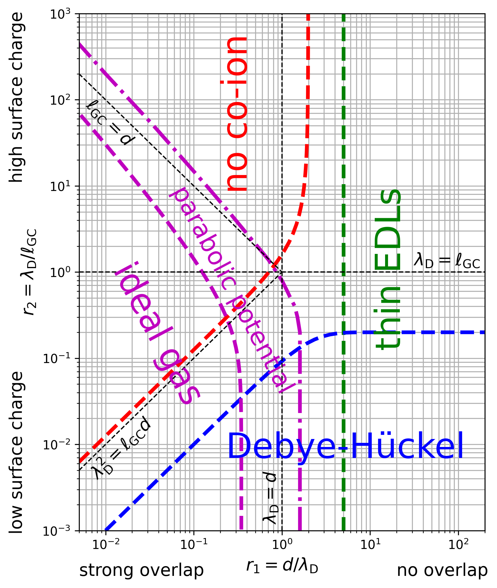
Figure 2: Domains of validity of the different approximate solutions to the PB equation for an electrolyte solution confined between two planar walls, as a function of the ratios $r_{1}=d/\lambda_{\text{D}}$ and $r_{2}=\lambda_{\text{D}}/\ell_{\text{GC}}$, where $d$ is the distance between the walls, $\lambda_{\text{D}}$ the Debye length, and $\ell_{\text{GC}}$ the Gouy-Chapman length.

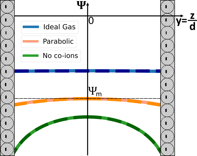
Figure 3: Typical potential profiles for an electrolyte solution confined between two planar walls, in the strong overlap regime ($r_{1}=d/\lambda_{\text{D}}=0.1$). Three limiting regimes are illustrated: ideal gas/homogeneous potential ($r_{2}=\lambda_{\text{D}}/\ell_{\text{GC}}=1$), parabolic potential ($r_{2}=10$), and no co-ion ($r_{2}=100$) limits. In the three cases, the exact potential (light continuous line) is compared to the approximated formula (dark dashed line) for the ideal gas, Eq. (46), parabolic potential, Eq. (50), and no co-ion, Eq. (51), limits.

IV.4.1 Thin EDLs limit

When the distance $d$ between the surfaces is much larger than the Debye length (corresponding to well-separated EDLs), one can solve the PB equation for a single charged wall (see Sec. IV.1), and superimpose the potentials of the two walls to obtain the full potential in the channel.

In practice, this approach provides an an accurate representation of the exact solution as long as $r_{1}=d/\lambda_{\text{D}}>5$. This boundary is represented with a green dashed line in Fig. 2.

IV.4.2 Debye-Hückel limit

In practice, the DH potential introduced in Sec. IV.3.2 is an excellent approximation to the exact potential as long as the surface potential, $|\psi_{\text{s}}|=\max(|\psi|)=|\psi(y=1/2)|$, remains under a (somehow arbitrary) critical value $\psi_{\text{c}}=0.4$. This corresponds to $r_{2}\leq\tanh(r_{1}/2)\times\psi_{\text{c}}/2$. This boundary is represented with a blue dashed line in Fig. 2.

One can then simplify the relation between $r_{1}$ and $r_{2}$ by considering two limits: for thin EDLs, $r_{1}\gg 1$, the DH solution can be used up to $r_{2}\leq\psi_{\text{c}}/2$; for overlapping EDLs, $r_{1}\ll 1$, the DH solution can be used up to $r_{2}\leq r_{1}\times\psi_{\text{c}}/4$.

IV.4.3 Homogeneous/parabolic potential limits

Homogeneous potential (ideal gas)

To estimate the range of validity of the homogeneous potential approximation (see Sec. IV.3.3), one can compare the homogeneous potential value to the next term in a Taylor series of the potential as a function of $z/\lambda_{\text{D}}$, i.e., the parabolic term.

The homogeneous potential writes: $|\psi_{\text{IG}}|=\text{asinh}(4r_{2}/r_{1})$, and the maximum difference between the parabolic term and its average value writes: $r_{1}r_{2}/3$. Imposing a maximum ratio $\theta_{\text{c}}$ between the two terms, one obtains:

$$r_{1}r_{2}=3\theta_{\text{c}}\text{asinh}\left(\frac{4r_{2}}{r_{1}}\right).$$ (53)

This boundary is represented for $\theta_{\text{c}}=1\,\%$ with a purple dashed line in Fig. 2.

Parabolic potential

The accuracy of the parabolic potential approximation depends crucially on the choice of $\psi_{\text{m}}$. Using $\psi_{\text{m}}=\psi_{\text{IG}}$, the error is approximately half the one of the homogeneous potential approximation, which does not extend much the range of parameters where it can be applied. In contrast, Eq. (50) approximates the exact potential within 1 % over a broader range of parameters, see the purple dashed-dotted line in Fig. 2.

IV.4.4 No co-ion limit

To determine the limits of applicability of this regime, one can estimate the ratio $\eta$ between counter-ions and co-ion densities in the middle of the channel:

$$\eta=\frac{n_{\text{m}}^{\text{counter-ion}}}{n_{\text{m}}^{\text{co-ion}}}=\exp{-2\psi_{\text{m}}}=\left(\frac{2r_{3}}{r_{1}}\right)^{4}.$$ (54)

One can consider that co-ions are efficiently excluded from the channel when $\eta$ is above a critical value $\eta_{\text{c}}$, that we will arbitrarily fix to $100$. Combining Eq. (52) and Eq. (54), one can see that $\eta=\eta_{\text{c}}$ corresponds to:

$$r_{2}=\frac{\eta_{\text{c}}^{1/4}}{2}\,\tan\left(\frac{r_{1}\eta_{\text{c}}^{1/4}}{4}\right).$$ (55)

This boundary is represented with a red dashed line in Fig. 2.

One can simplify the relation between $r_{1}$ and $r_{2}$ by considering two limits: for small surface charges, $r_{2}\ll 1$, the no co-ion approximation can be used for $r_{2}\geq r_{1}\eta_{\text{c}}^{1/2}/8\approx 1.25r_{1}$; for large surface charges, $r_{2}\gg 1$, the no co-ion approximation can be used for $r_{1}\leq 2\pi/\eta_{\text{c}}^{1/4}\approx 1.99$.

V Cylindrical channel

This section gathers the equations describing a $Z$:$Z$ electrolyte solution confined inside a cylindrical channel of radius $R$, see Fig. 1(d). More detailed discussions can be found in e.g. Refs. 13, 14, 15.

V.1 Thin EDL

When the channel radius $R$ is much larger than the thickness of the EDL, one can neglect the wall curvature at the scale of the EDL, and solve the PB equation for a single planar charged wall, see section IV.1, where the distance to the wall is $z=R-r$.

Accordingly, the integrals computed per unit surface for a single planar wall in Sec. IV.1.4 can simply be multiplied by $2\pi R$ to obtain the corresponding integral per unit length of the cylindrical channel.

The limits of validity of this approximation will be quantified in section V.4.

V.2 Thick EDL, high surface charge: no co-ion

When the EDLs overlap and for large enough surface charges (these conditions will be quantified in section V.4), co-ions are excluded from the channel and the PB equation can be solved with counter-ions only.

V.2.1 PB equation: derivation

As for the slit channel, the counter-ion density is denoted $n(r)$, and one can define an auxiliary reduced potential $\psi$, which is always negative:

$$\psi=-\text{sgn}(\Sigma)\times\phi=-\text{sgn}(\Sigma)\times\beta qV.$$

The potential in the middle of the channel is arbitrarily fixed to zero: $\psi_{\text{m}}=\psi(r=0)=0$ (this condition will be relaxed in section V.3.3). Denoting $n_{\text{m}}$ the counter-ion density at $r=0$, one can define the same characteristic length $K^{-1}$ as for the slit geometry,

$$K^{-1}=\frac{1}{\sqrt{2\pi\ell_{\text{B}}n_{\text{m}}}}\quad\Leftrightarrow\quad n_{\text{m}}=\frac{K^{2}}{2\pi\ell_{\text{B}}},$$

and derive the PB equation for a negative surface charge (with positive counter-ions) or for a positive surface charge (with negative counter-ions).

Poisson equation:

$$qn(r)=-\dfrac{\varepsilon}{\beta q}\,\frac{1}{r}\frac{\mathrm{d}}{\mathrm{d}r}\left(r\frac{\mathrm{d}\psi}{\mathrm{d}r}\right)$$

Boltzmann distribution:

$$n(r)=n_{\text{m}}\,\mathrm{e}^{-\psi(r)}$$

Poisson-Boltzmann equation:

$$\frac{1}{r}\frac{\mathrm{d}}{\mathrm{d}r}\left(r\frac{\mathrm{d}\psi}{\mathrm{d}r}\right)=-2K^{2}\,\mathrm{e}^{-\psi(r)}$$ (56)

V.2.2 PB equation: solution

$$\psi(r)=2\ln\left[1-\left(\frac{Kr}{2}\right)^{2}\right]$$ (57)

$$\dfrac{\mathrm{d}\psi}{\mathrm{d}r}=\frac{-K^{2}r}{1-\left(\frac{Kr}{2}\right)^{2}}$$ (58)

$$n(r)=\dfrac{n_{\text{m}}}{\left[1-\left(\frac{Kr}{2}\right)^{2}\right]^{2}}=\dfrac{K^{2}}{2\pi\ell_{\text{B}}\left[1-\left(\frac{Kr}{2}\right)^{2}\right]^{2}}$$ (59)

V.2.3 Surface charge and surface potential

To fully determine the potential and ion density profiles, one needs to express $K$ as a function of the surface charge.

Electrostatics at the interface (or equivalently, global electroneutrality):

$$\left.\frac{\mathrm{d}V}{\mathrm{d}r}\right|_{r=R}=\frac{\Sigma}{\varepsilon}\quad\Rightarrow\quad\left.\frac{\mathrm{d}\psi}{\mathrm{d}r}\right|_{r=R}=-\frac{2}{\ell_{\text{GC}}}$$ (60)

Using Eq. (58), one obtains:

$$\frac{(KR)^{2}}{1-\left(\frac{KR}{2}\right)^{2}}=\frac{2R}{\ell_{\text{GC}}},$$ (61)

which can be solved:

$$\frac{KR}{2}=\sqrt{\frac{R/\ell_{\text{GC}}}{R/\ell_{\text{GC}}+2}}.$$ (62)

Hence, in contrast with the slit geometry, an explicit expression of $K$ can be derived in general for a cylindrical channel.

V.2.4 A few integrals

Electrostatic energy $\mathcal{E}$ (per unit length of the channel)

Denoting $y=KR/2$,

$$\mathcal{E}=\frac{\varepsilon}{2}\int_{0}^{R}2\pi r\,\mathrm{d}r\ \left(\frac{\mathrm{d}V}{\mathrm{d}r}\right)^{2}\\ =\frac{2}{\ell_{\text{B}}\beta}\left[\ln(1-y^{2})+\frac{y^{2}}{1-y^{2}}\right]$$ (63)

Using Eq. (62), $\mathcal{E}$ can be directly written in terms of $R/\ell_{\text{GC}}$:

$$\mathcal{E}=\frac{2}{\ell_{\text{B}}\beta}\left[\ln(\frac{2}{R/\ell_{\text{GC}}+2})+\frac{R}{2\ell_{\text{GC}}}\right]$$ (64)

Ionic density

$$\int_{0}^{R}2\pi r\,\mathrm{d}r\ n(z)=2\pi R\frac{|\Sigma|}{q}=\frac{R}{\ell_{\text{B}}\ell_{\text{GC}}}$$ (65)

V.2.5 Low and high surface charge limits

Low surface charge

When $\Sigma$ is small enough that $R/\ell_{\text{GC}}\ll 1$, Eq. (62) simplifies:

$$KR\approx\sqrt{2R/\ell_{\text{GC}}},$$ (66)

which is accurate to within 1 % up to $R/\ell_{\text{GC}}\approx 0.04$.

Note that when $R/\ell_{\text{GC}}\ll 1$, $KR\ll 1$, so that $\psi\approx 0$ and the ion density is approximately homogeneous in the channel:

$$n\approx\dfrac{K^{2}}{2\pi\ell_{\text{B}}}=\dfrac{1}{\pi R\ell_{\text{B}}\ell_{\text{GC}}}.$$ (67)

This is commonly called the ideal gas regime. In practice, the ion density varies by less than 10 % over the channel thickness as long as $R/\ell_{\text{GC}}<0.1$.

High surface charge

When $\Sigma$ is large enough that $R/\ell_{\text{GC}}\gg 1$, Eq. (62) simplifies:

$$KR\approx\frac{2}{1+\frac{\ell_{\text{GC}}}{R}},$$ (68)

which is accurate to within 1 % down to $R/\ell_{\text{GC}}\approx 7$.

Eventually, when $R/\ell_{\text{GC}}\rightarrow\infty$, $KR\rightarrow 2$, and the potential and ion density profiles reach a limit, sometimes referred to as the “Gouy-Chapman limit”:

$$\psi(r)=2\ln\left[1-\left(\frac{r}{R}\right)^{2}\right],$$ (69)

$$n(r)=\dfrac{2}{\pi\ell_{\text{B}}R^{2}\left[1-\left(\frac{r}{R}\right)^{2}\right]^{2}}.$$ (70)

V.3 General case

In a cylindrical channel, we are not aware of a usable analytical solution for the general case, and the PB equation has to be solved numerically (a Python script to that aim is provided in the appendix, A.2). Nevertheless, like in the slit case, one can define two ratios $r_{1}=R/\lambda_{\text{D}}$ and $r_{2}=\lambda_{\text{D}}/\ell_{\text{GC}}$, which uniquely determine the auxiliary reduced potential $\psi=-\text{sgn}(\Sigma)\times\phi$ expressed as a function of the reduced position $y=r/R$. Different approximate solutions can be written depending on $r_{1}$ and $r_{2}$, discussed in the following.

V.3.1 Debye-Hückel limit

When the reduced potential $|\psi|$ is small everywhere, the PB equation can be linearized (DH regime).

With the conditions:

$$\left.\frac{\mathrm{d}\psi}{\mathrm{d}r}\right|_{r=0}=0\quad\text{and}\quad\left.\frac{\mathrm{d}\psi}{\mathrm{d}r}\right|_{r=R}=-\frac{2}{\ell_{\text{GC}}},$$

the solution to the linearized PB equation in cylindrical coordinates, $\frac{1}{r}\frac{\mathrm{d}}{\mathrm{d}r}\left(r\frac{\mathrm{d}\psi}{\mathrm{d}r}\right)=\psi/\lambda_{\text{D}}^{2}$, writes:

$$\psi(r)=-\frac{2\lambda_{\text{D}}}{\ell_{\text{GC}}}\ \frac{\mathrm{I}_{0}\left(\frac{r}{\lambda_{\text{D}}}\right)}{\mathrm{I}_{1}\left(\frac{R}{\lambda_{\text{D}}}\right)}=-2r_{2}\frac{\mathrm{I}_{0}\left(r_{1}y\right)}{\mathrm{I}_{1}\left(r_{1}\right)},$$ (71)

where $\mathrm{I}_{0}(x)$ and $\mathrm{I}_{1}(x)$ are the modified Bessel functions of the first kind of order zero and one. The corresponding potential $V$ writes:

$$V(r)=\frac{\Sigma\lambda_{\text{D}}}{\varepsilon}\ \frac{\mathrm{I}_{0}\left(\frac{r}{\lambda_{\text{D}}}\right)}{\mathrm{I}_{1}\left(\frac{R}{\lambda_{\text{D}}}\right)}.$$ (72)

The limits of validity of this approximation will be quantified in section V.4.

Electrostatic energy $\mathcal{E}$ (per unit length of the cylindrical channel)

With $y=R/\lambda_{\text{D}}$,

$$\begin{split}\mathcal{E}&=\frac{\varepsilon}{2}\int_{0}^{R}2\pi r\left(\frac{\differential V}{\differential r}\right)^{2}\differential r\\ &=\frac{R^{2}}{2\beta\ell_{\text{B}}\ell_{\text{GC}}^{\,2}}\left[1-\frac{I_{0}(y)I_{2}(y)}{I_{1}(y)^{2}}\right].\end{split}$$ (73)

V.3.2 Homogeneous/parabolic potential limits

Homogeneous potential

When the EDLs overlap ($r_{1}=R/\lambda_{\text{D}}\ll 1$) and for low enough surface charges ($r_{1}r_{2}=R/\ell_{\text{GC}}\ll 1$), the potential and ion densities are almost homogeneous: this is commonly referred to as the ideal gas limit. In this limit, the ion densities and the auxiliary reduced potential write:

$$\begin{split}n^{\text{IG}}_{\pm}&=\mp\frac{\Sigma}{qR}+\sqrt{n_{0}^{2}+\left(\frac{\Sigma}{qR}\right)^{2}}\\ &=n_{0}\left\{\mp\text{sgn}(\Sigma)\frac{\ell_{\text{Du}}}{R}+\sqrt{1+\left(\frac{\ell_{\text{Du}}}{R}\right)^{2}}\right\},\end{split}$$ (74)

$$\psi_{\text{IG}}=-\text{asinh}\left(\frac{\ell_{\text{Du}}}{R}\right)=-\text{asinh}\left(\frac{4r_{2}}{r_{1}}\right),$$ (75)

introducing the Dukhin length $\ell_{\text{Du}}=(|\Sigma|/q)/n_{0}=4\lambda_{\text{D}}^{2}/\ell_{\text{GC}}$. The limits of validity of this approximation will be discussed in section V.4.

Parabolic potential

For weaker EDL overlaps, one can expand the solution of the PB equation in series of $r/\lambda_{\text{D}}$; to second order, one obtains [12]:

$$\psi(r)\approx\psi_{\text{m}}+\frac{\text{sinh}(\psi_{\text{m}})}{4}\left(\frac{r}{\lambda_{\text{D}}}\right)^{2}.$$ (76)

Using $\psi_{\text{m}}=\psi_{\text{IG}}$, one gets:

$$\psi(r)\approx-\text{asinh}\left(\frac{4r_{2}}{r_{1}}\right)-\frac{r_{2}}{r_{1}}\left(\frac{r}{\lambda_{\text{D}}}\right)^{2}.$$ (77)

However, the ideal gas potential is close to the average potential in the channel, and systematically shifted from the potential in the middle of the channel. The shift can be estimated as:

$$\frac{1}{\pi R^{2}}\int_{0}^{R}-\frac{r_{2}}{r_{1}}\left(\frac{r}{\lambda_{\text{D}}}\right)^{2}2\pi r\differential r\approx-\frac{r_{1}r_{2}}{2},$$

and it can be subtracted from $\psi_{\text{IG}}$ to obtain a closer approximation to $\psi_{\text{m}}$:

$$\psi_{\text{IG}}^{\text{cor}}=-\text{asinh}\left(\frac{4r_{2}}{r_{1}}\right)+\frac{r_{1}r_{2}}{2}.$$ (78)

Overall, a good practical approximation for $\psi(r)$ is:

$$\begin{split}\psi(r)&\approx\psi_{\text{IG}}^{\text{cor}}+\frac{\text{sinh}(\psi_{\text{IG}})}{4}\left(\frac{r}{\lambda_{\text{D}}}\right)^{2}\\ &=-\text{asinh}\left(\frac{4r_{2}}{r_{1}}\right)+\frac{r_{1}r_{2}}{2}-\frac{r_{2}}{r_{1}}\left(\frac{r}{\lambda_{\text{D}}}\right)^{2}.\end{split}$$ (79)

The limits of validity of this approximation will be discussed in section V.4.

V.3.3 No co-ion limit

When the EDL extends over the whole channel and for large enough surface charges, co-ions are excluded from the channel and the PB equation can be solved with counter-ions only, see Sec. V.2. The auxiliary reduced potential $\psi(r)$ and the counter-ion density profile $n(r)$ were given by Eq. (57) and by Eq. (59), respectively. Both $\psi$ and $n$ depended on an inverse length $K$ related to the surface charge via Eq. (62).

However, the potential in the middle of the channel was arbitrarily fixed to zero. To reproduce the exact potential, one needs to acknowledge that the channel is connected to an external salt reservoir with salt concentration $n_{0}$ and corresponding Debye length $\lambda_{\text{D}}$. Moving the reference of potential to the reservoir, $\psi_{0}=0$, the Boltzmann distribution for the counter-ions becomes $n(z)=n_{0}\,\mathrm{e}^{-\psi(z)}$, and the PB equation rewrites:

$$\frac{1}{r}\frac{\mathrm{d}}{\mathrm{d}r}\left(r\frac{\mathrm{d}\psi}{\mathrm{d}r}\right)=-\frac{1}{2\lambda_{\text{D}}^{2}}\,\mathrm{e}^{-\psi(r)},$$

$$\text{with}\ \ \left.\frac{\mathrm{d}\psi}{\mathrm{d}r}\right|_{r=0}=0\ \ \text{and}\ \ \left.\frac{\mathrm{d}\psi}{\mathrm{d}r}\right|_{r=R}=-\frac{2}{\ell_{\text{GC}}}.$$

Denoting $KR=r_{3}$, the solution writes:

$$\psi=2\ln\left\{\frac{r_{1}}{2r_{3}}\left[1-\left(\frac{r_{3}y}{2}\right)^{2}\right]\right\},$$ (80)

with

$$r_{3}=2\sqrt{\frac{r_{1}r_{2}}{r_{1}r_{2}+2}}.$$ (81)

In particular, the potential in the center of the channel is $\psi_{\text{m}}=\psi(y=0)=2\ln\left[r_{1}/(2r_{3})\right]$. The limits of validity of this approximation will be discussed in section V.4.

V.4 Validity of the approximate solutions

We will in the following bound the regions in the $r_{1}-r_{2}$ diagram where the different approximate solutions can be used safely, see Fig. 4.

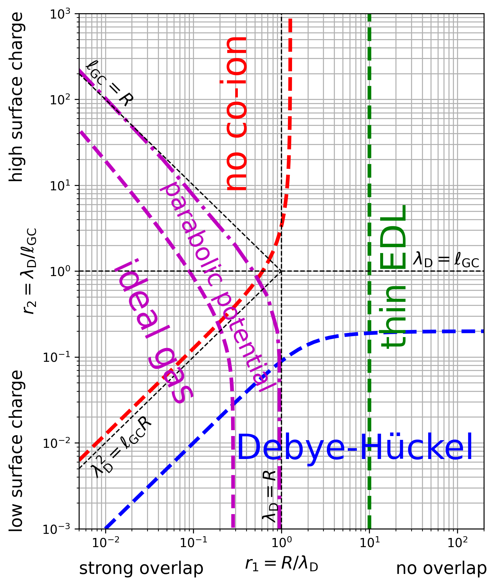
Figure 4: Domains of validity of the different approximate solutions to the PB equation for an electrolyte solution confined inside a cylindrical channel, as a function of the ratios $r_{1}=R/\lambda_{\text{D}}$ and $r_{2}=\lambda_{\text{D}}/\ell_{\text{GC}}$, where $R$ is the channel radius, $\lambda_{\text{D}}$ the Debye length, and $\ell_{\text{GC}}$ the Gouy-Chapman length.

V.4.1 Thin EDL limit

When the channel radius $R$ is much larger than $\lambda_{\text{D}}$, one can neglect the wall curvature at the scale of the EDL, and solve the PB equation for a single planar charged wall.

However this approximation should be taken with caution. Even when the EDL is significantly thinner than the channel radius ($R/\lambda_{\text{D}}>10$), the planar wall solution only provides a fair description of the exact potential profile. Still, this boundary is represented with a green dashed line in Fig. 2.

V.4.2 Debye-Hückel limit

Like in the slit case, the DH potential introduced in Sec. V.3.1 is an excellent approximation to the exact potential as long as the surface potential, $|\psi_{\text{s}}|=\max(|\psi|)=|\psi(r=R)|$ remains under a (somehow arbitrary) critical value $\psi_{\text{c}}=0.4$. This corresponds to:

$$r_{2}\leq\frac{\mathrm{I}_{1}(r_{1})}{\mathrm{I}_{0}(r_{1})}\times\frac{\psi_{\text{c}}}{2}.$$ (82)

This boundary is represented with a blue dashed line in Fig. 4.

One can then simplify the relation between $r_{1}$ and $r_{2}$ by considering two limits: for thin EDLs, $r_{1}\gg 1$, the DH solution can be used up to $r_{2}\leq\psi_{\text{c}}/2$; for overlapping EDLs, $r_{1}\ll 1$, the DH solution can be used up to $r_{2}\leq r_{1}\times\psi_{\text{c}}/4$.

V.4.3 Homogeneous/parabolic potential limits

Homogeneous potential (ideal gas)

To estimate the range of validity of the homogeneous potential approximation (see Sec. V.3.2), one can compare the homogeneous potential value to the next term in a Taylor series of the potential as a function of $R/\lambda_{\text{D}}$, i.e., the parabolic term.

The homogeneous potential writes: $|\psi_{\text{IG}}|=\text{asinh}(4r_{2}/r_{1})$, and the maximum difference between the parabolic term and its average value writes: $r_{1}r_{2}/2$. Imposing a maximum ratio $\theta_{\text{c}}$ between the two terms, one obtains:

$$r_{1}r_{2}=2\theta_{\text{c}}\text{asinh}\left(\frac{4r_{2}}{r_{1}}\right).$$ (83)

This boundary is represented for $\theta_{\text{c}}=1\,\%$ with a purple dashed line in Fig. 4.

Parabolic potential

The accuracy of the parabolic potential approximation depends crucially on the choice of $\psi_{\text{m}}$. Using $\psi_{\text{m}}=\psi_{\text{IG}}$, the error is approximately the same as the one of the homogeneous potential approximation. In contrast, Eq. (79) approximates the exact potential within 1 % over a broader range of parameters, see the purple dashed-dotted line in Fig. 4.

V.4.4 No co-ion limit

To determine the limits of applicability of this regime, one can estimate the ratio $\eta$ between counter-ions and co-ion densities in the middle of the channel:

$$\eta=\frac{n_{\text{m}}^{\text{counter-ion}}}{n_{\text{m}}^{\text{co-ion}}}=\exp{-2\psi_{\text{m}}}=\left(\frac{2r_{3}}{r_{1}}\right)^{4}.$$ (84)

One can consider that co-ions are efficiently excluded from the channel when $\eta$ is above a critical value $\eta_{\text{c}}$, that we will arbitrarily fix to $100$. Combining Eq. (81) and Eq. (84), one can see that $\eta=\eta_{\text{c}}$ corresponds to:

$$r_{2}=\frac{2r_{1}\eta_{\text{c}}^{1/2}}{16-r_{1}^{\,2}\eta_{\text{c}}^{1/2}}.$$ (85)

This boundary is represented with a red dashed line in Fig. 4.

One can simplify the relation between $r_{1}$ and $r_{2}$ by considering two limits: for small surface charges, $r_{2}\ll 1$, the no co-ion approximation can be used for $r_{2}\geq r_{1}\eta_{\text{c}}^{1/2}/8\approx 1.25r_{1}$; for large surface charges, $r_{2}\gg 1$, the no co-ion approximation can be used for $r_{1}\leq 4/\eta_{\text{c}}^{1/4}\approx 1.26$.

VI Common boundary conditions

VI.1 Surface charge density and surface potential

At a charged surface, the surface charge density $\Sigma$ and the surface potential $\phi_{\text{s}}$ can be linked by expressing the electric field at the wall as a function of the surface charge, Eq. (10). This equation can be solved when the shape of the potential is known, resulting e.g. in the Grahame equation, Eq. (11), for one wall with salt.

VI.2 Constant charge

Insulating walls are commonly described using a constant surface charge, i.e., the surface charge density $\Sigma$ is imposed. This is the boundary condition considered by default in this formulary. The surface potential $\phi_{\text{s}}$ can then be obtained from interfacial electrostatics, see Sec. VI.1.

VI.3 Constant potential

In contrast, conducting surfaces are usually described using a constant potential, i.e., the surface potential $\phi_{\text{s}}$ is imposed. All the results in the formulary can be expressed in terms of the surface potential $\phi_{\text{s}}$ and/or $\gamma=\tanh(\phi_{\text{s}}/4)$, through the relation between $\phi_{\text{s}}$ and $\Sigma$ given by interfacial electrostatics, see Sec. VI.1.

The domains of validity of the different approximations can also be represented, e.g. for a slit channel, as a function of $r_{1}=d/\lambda_{\text{D}}$ and $|\phi_{\text{s}}|$, see Fig. 5.

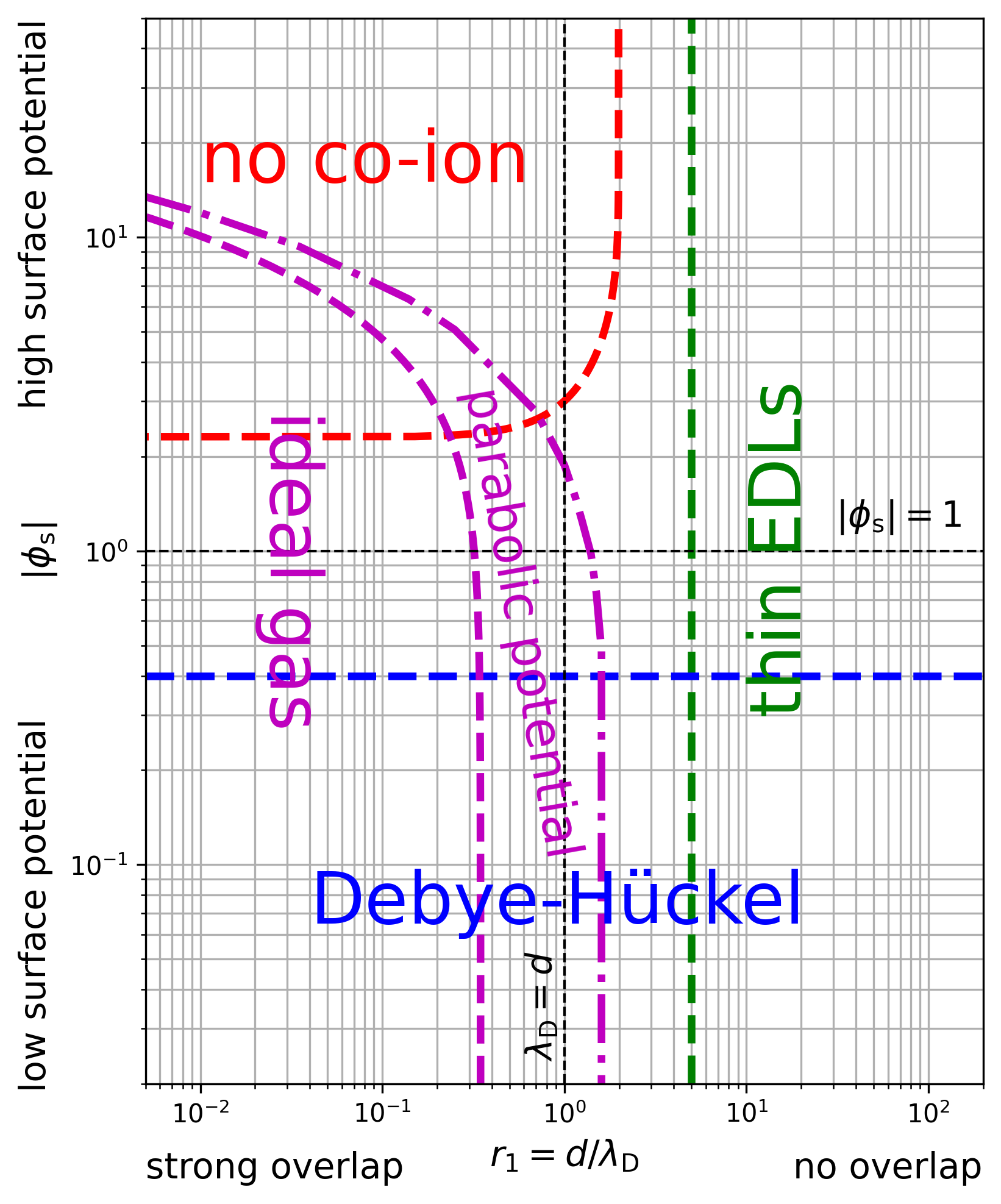
Figure 5: Domains of validity of the different approximate solutions to the PB equation for an electrolyte solution confined between two planar walls, as a function of $r_{1}=d/\lambda_{\text{D}}$ and $|\phi_{\text{s}}|$, where $d$ is the distance between the walls, $\lambda_{\text{D}}$ the Debye length, and $\phi_{\text{s}}$ the reduced surface potential.

VI.4 Charge regulation

Finally, surface charge and potential can be controlled by chemical reactions at the surface, for instance in the presence of ionizable groups at the surface, which can release counter-ions into the solution [16]. We will present here the simple and common case of a single-site dissociation process, described by the reaction:

$$\ce{AB<-->A^{-}+B^{+}},$$ (86)

where $\ce{AB}$ denotes a neutral surface site that can be ionized, $\ce{A^{-}}$, releasing a counter-ion $\ce{B^{+}}$ in solution (we arbitrarily consider a negatively charged surface, and monovalent ionized sites). This process is characterized by an equilibrium constant $K_{\text{d}}$ through:

$$K_{\text{d}}=\frac{[\ce{A^{-}}][\ce{B^{+}}]_{\text{s}}}{[\ce{AB}]},$$ (87)

where $[\ce{A^{-}}]$, $[\ce{B^{+}}]_{\text{s}}$, and $[\ce{AB}]$ denote the concentrations of the species at the surface.

Denoting $a$ the average distance between the ionizable sites on the surface, one can relate the fraction of ionized groups $\varphi_{\text{A}}$ to the surface charge: $\varphi_{\text{A}}=-\Sigma a^{2}/e$. $\varphi_{\text{A}}$ is also related to the concentrations of $\ce{AB}$ and $\ce{A^{-}}$ at the surface through: $[\ce{A^{-}}]/[\ce{AB}]=\varphi_{\text{A}}/(1-\varphi_{\text{A}})$.

The concentration of $\ce{B^{+}}$ at the interface can then be expressed as a function of the surface potential, and Eq. (87) provides a relation between the surface charge and the surface potential. Formally, denoting $n_{\text{B}}^{\text{bulk}}$ the concentration of $\ce{B^{+}}$ in bulk, $[\ce{B^{+}}]_{\text{s}}=n_{\text{B}}^{\text{bulk}}\exp(-\phi_{\text{s}})$, and Eq. (87) can be rewritten:

$$\varphi_{\text{A}}=-\frac{\Sigma a^{2}}{e}=\frac{1}{1+\frac{1}{K_{\text{d}}}n_{\text{B}}^{\text{bulk}}\exp(-\phi_{\text{s}})}.$$ (88)

Finally, interfacial electrostatics provides another relation between surface charge and surface potential (e.g. Grahame equation, Eq. (11), for one wall with salt), so that $\Sigma$ and $\phi_{\text{s}}$ can be uniquely determined by combining the two equations.

VII Limits of the PB framework

In the first molecular layers of liquid close to the wall, the hypotheses underlying the PB equation generally fail. The reader can find detailed discussions on the limits of the PB theory in e.g. Refs. 1, 2, 3, 9, 10, 4, 5, 17, 7, 18, 8.

Here we will simply present a criterion for the validity of the mean field approximation. The importance of ionic correlations can be quantified by the plasma parameter $\Gamma$, see Refs. 19, 20, 21, which compares the typical interaction energy between two ions and the thermal energy $k_{\mathrm{B}}T$:

$$\Gamma=\frac{\beta q^{2}}{4\pi\varepsilon d_{\mathrm{ion}}}=\frac{\ell_{\text{B}}}{d_{\mathrm{ion}}},$$ (89)

where $d_{\mathrm{ion}}$ is the typical inter-ionic distance.

This typical inter-ionic distance can be related to surface or bulk properties, imposing respectively a critical surface charge density $|\Sigma|^{\mathrm{c}}$ or a critical salt concentration $n_{0}^{\mathrm{c}}$ above which the applicability of the PB framework should be taken with care.

At the surface, assuming that counter-ions organize into a monolayer screening the surface charge, $1/d_{\mathrm{ion}}^{\,2}=|\Sigma|/q$, and $\Gamma^{\text{surface}}=\sqrt{|\Sigma|\ell_{\text{B}}^{2}/q}$. Ionic correlations cannot be neglected when $\Gamma^{\text{surface}}>1$, see Refs. 19, 20, corresponding to:

$$|\Sigma|>|\Sigma|^{\mathrm{c}}=\frac{q}{\ell_{\text{B}}^{2}}=\frac{(4\pi\varepsilon/\beta)^{2}}{(Ze)^{3}},$$ (90)

where the last expression highlights the strong impact of the ion valence $Z$ on $\absolutevalue{\Sigma^{\mathrm{c}}}$. For monovalent ions in water at $300\,$K, $\absolutevalue{\Sigma^{\mathrm{c}}}\sim 330\,$mC/m², but for divalent ions it drops to $\sim 40\,$mC/m².

In bulk, because the total ionic concentration is twice the salt concentration, the inter-ionic distance is $d_{\mathrm{ion}}=(2n_{0})^{-1/3}$, and $\Gamma^{\text{bulk}}=(2n_{0}\ell_{\text{B}}^{3})^{1/3}$. Ionic correlations cannot be neglected when $\Gamma^{\text{bulk}}>1$, see Refs. 19, 20, corresponding to:

$$n_{0}>n_{0}^{\mathrm{c}}=\frac{1}{2\ell_{\text{B}}^{3}}=\frac{(4\pi\varepsilon/\beta)^{3}}{2(Ze)^{6}}.$$ (91)

For a monovalent salt in water at $300\,$K, $n_{0}^{\mathrm{c}}\sim 2\,$M, but for a divalent salt it drops to $\sim 30$ mM.

Finally, it is important to note that, for monovalent ions in water at room temperature, $\ell_{\text{B}}\sim 7\,$Å is greater than the ionic size, so that there will be no steric repulsion effects when $\Gamma=\ell_{\text{B}}/d_{\mathrm{ions}}<1$.

Appendix A Numerical solution with Python

The Python codes listed below solve numerically the PB equation in the slit and cylindrical geometries, using the solve_bvp function of the SciPy package. The script files are included in the sources of this archive.

A.1 Slit channel

This code computes and plots the auxiliary reduced potential $\psi=-\text{sgn}(\Sigma)\times\phi$ as a function of the reduced position $z/d$ in a slit channel with walls located at $z=-d/2$ and $z=d/2$ (see Sec. IV.3), for a broad range of values of $r_{1}=d/\lambda_{\text{D}}$ and $r_{2}=\lambda_{\text{D}}/\ell_{\text{GC}}$.

In order to use the solve_bvp function, one needs to convert the PB equation into a first order system of ordinary differential equations subject to two-point boundary conditions:

$$\frac{\differential^{2}\psi}{\differential z^{2}}=\frac{1}{\lambda_{\text{D}}^{2}}\sinh\{\psi\}\quad\text{with}\quad\left.\frac{\differential\psi}{\differential z}\right|_{z=0}=0\quad\text{and}\quad\left.\frac{\differential\psi}{\differential z}\right|_{z=d/2}=-\frac{2}{\ell_{\text{GC}}}$$

$$x=z/d,\quad y_{0}=\psi,\quad r_{1}=d/\lambda_{\text{D}},\quad r_{2}=\lambda_{\text{D}}/\ell_{\text{GC}}\quad\Rightarrow\left\{\begin{aligned} &y_{0}^{\prime}=y_{1}\\ &y_{1}^{\prime}=r_{1}^{2}\sinh(y_{0})\end{aligned}\right.\quad\text{with}\quad\left\{\begin{aligned} &y_{1}(0)=0\\ &y_{1}(1/2)=-2r_{1}r_{2}\end{aligned}\right.$$

Listing 1: PB_slit_num.py

⬇

#!/usr/bin/env python3

# -*- coding: utf-8 -*-

r1 = 5.

r2 = 5.

import numpy as np

import matplotlib.pyplot as plt

from scipy.integrate import solve_bvp

# y0 = psi

# x = z/d

# Right-hand side of the system:

# y0’ = y1

# y1’ = r1^2 sinh(y0)

def fun(x, y):

return np.vstack((y[1], r1**2*np.sinh(y[0])))

# Boundary conditions:

# y1(left) = 0

# y1(right)+2r1r2 = 0

def bc(ya, yb):

return np.array([ya[1], yb[1]+2.0*r1*r2])

# Solving for x in [0;0.5]

x = np.linspace(0., 0.5, 10000)

y = np.zeros((2, x.size))

# Initial guess for the potential profile

r1init = 1.

r3init = 3.135322030076839 # r2init = 1000

y[0] = 2.*np.log(r1init/(2.*r3init)*np.cos(r3init*x))

# Calling solve_bvp

res = solve_bvp(fun, bc, x, y, tol=1.e-6, max_nodes=5000000)

x_plot = np.linspace(0., 0.5, 500)

y_plot = res.sol(x_plot)[0]

plt.plot(x_plot, y_plot, label=’numerical’)

plt.legend()

plt.xlabel(r”$z/d$”)

plt.ylabel(r”$\psi$”)

plt.show()

A.2 Cylindrical channel

This code computes and plots the auxiliary reduced potential $\psi=-\text{sgn}(\Sigma)\times\phi$ as a function of the reduced position $r/R$ in a cylindrical channel of radius $R$ (see Sec. V.3), for a broad range of values of $r_{1}=R/\lambda_{\text{D}}$ and $r_{2}=\lambda_{\text{D}}/\ell_{\text{GC}}$.

In order to use the solve_bvp function, one needs to convert the PB equation into a first order system of ordinary differential equations subject to two-point boundary conditions:

$$\frac{\differential^{2}\psi}{\differential r^{2}}+\frac{1}{r}\frac{\differential\psi}{\differential r}=\frac{1}{\lambda_{\text{D}}^{2}}\sinh\{\psi\}\quad\text{with}\quad\left.\frac{\differential\psi}{\differential r}\right|_{r=0}=0\quad\text{and}\quad\left.\frac{\differential\psi}{\differential r}\right|_{r=R}=-\frac{2}{\ell_{\text{GC}}}$$

$$x=r/R,\quad y_{0}=\psi,\quad r_{1}=R/\lambda_{\text{D}},\quad r_{2}=\lambda_{\text{D}}/\ell_{\text{GC}}\quad\Rightarrow\left\{\begin{aligned} &y_{0}^{\prime}=y_{1}\\ &y_{1}^{\prime}=r_{1}^{2}\sinh(y_{0})-y_{1}/x\end{aligned}\right.\quad\text{with}\quad\left\{\begin{aligned} &y_{1}(0)=0\\ &y_{1}(1)=-2r_{1}r_{2}\end{aligned}\right.$$

Listing 2: PB_cyl_num.py

⬇

#!/usr/bin/env python3

# -*- coding: utf-8 -*-

r1 = 5.

r2 = 5.

import numpy as np

import matplotlib.pyplot as plt

from scipy.integrate import solve_bvp

# y0 = psi

# x = r/R

# Right-hand side of the system:

# y0’ = y1

# y1’ = r1^2 sinh(y0)-y1/x

def fun(x, y):

return np.vstack((y[1], r1**2*np.sinh(y[0])-y[1]/x))

# Boundary conditions:

# y1(left) = 0

# y1(right)+2r1r2 = 0

def bc(ya, yb):

return np.array([ya[1], yb[1]+2.0*r1*r2])

# Solving for x in ]0;1]

x = np.linspace(1.e-6, 1., 10000)

y = np.zeros((2, x.size))

# Initial guess for the potential profile

r1init = 1.

r3init = 1.9980029950087341 # r2init = 1000

y[0] = 2.*np.log(r1init/(2.*r3init)*(1.-(r3init*x/2)**2))

# Calling solve_bvp

res = solve_bvp(fun, bc, x, y, tol=1.e-6, max_nodes=5000000)

x_plot = np.linspace(0., 1., 500)

y_plot = res.sol(x_plot)[0]

plt.plot(x_plot, y_plot, label=’numerical’)

plt.legend()

plt.xlabel(r”$r/R$”)

plt.ylabel(r”$\psi$”)

plt.show()