Channel linear Weingarten surfaces in space forms

Abstract.

Channel linear Weingarten surfaces in space forms are investigated in a Lie sphere geometric setting, which allows for a uniform treatment of different ambient geometries. We show that any channel linear Weingarten surface in a space form is isothermic and, in particular, a surface of revolution in its ambient space form.

We obtain explicit parametrisations for channel surfaces of constant Gauss curvature in space forms, and thereby for a large class of linear Weingarten surfaces up to parallel transformation.

1. Introduction

Two different ways to define linear Weingarten surfaces can be found in the literature, either by requiring an affine relationship between the principal curvatures or one between the mean and the Gauss curvature. In these notes, we adopt the second definition: a surface in a space form is called linear Weingarten if, for some non-trivial triple $a,b,c\in\mathbb{R}$, its Gauss and mean curvatures $K$ and $H$ satisfy

$$aK+2bH+c=0.$$

This includes surfaces of constant Gauss or mean curvature (CGC or CMC, respectively) as well as their parallel surfaces.

We investigate linear Weingarten surfaces that are additionally channel surfaces, that is, envelop a $1$-parameter family of spheres. An example is provided by surfaces that are invariant under a $1$-parameter subgroup of rotations in the given space form. The study of such rotational linear Weingarten surfaces goes back to Delaunay’s investigations of CMC surfaces of revolution in Euclidean space in [12], but have again sparked interest in recent years from various points of view, see [3], [24], [25] or most recently [2], [16], [27] and references therein. Since the considered surfaces arise via the action of isometries on a planar profile curve, all curvature notions only depend on the profile curve. This fact has been used to prove various classification results for these curves and, subsequently, rotational linear Weingarten surfaces. However, explicit parametrisation formulas for these surfaces seem only to be available in special cases.

Channel linear Weingarten surfaces in Euclidean space are either tubular or surfaces of revolution, and are parallel to either the catenoid or a CGC surface, as was shown in [20] by giving explicit parametrisations in terms of Jacobi’s elliptic functions ([1, Chap. 16]). In this way, the authors obtained a complete and transparent classification of channel linear Weingarten surfaces in Euclidean space.

In this present text, we aim to complement the existing results by explicit parametrisations for rotational CGC surfaces, in particular, in hyperbolic space $\mathbb{H}^{3}$ and the $3$-sphere $\mathbb{S}^{3}$ and, in consequence, for any linear Weingarten surface that is parallel to such a CGC surface — the clear advantage being that many results about such surfaces can then be derived or verified by mere computation. Particular attention is paid to a choice of parametrisations that are well-behaved across singularities of the surfaces, that necessarily occur in various cases according to Hilbert’s theorem. Our parametrisations provide a complete classification result for non-tubular channel linear Weingarten surfaces in $\mathbb{S}^{3}$, where every such surface is parallel to a CGC surface (cf [3]), and encompass the large class of channel linear Weingarten surfaces in $\mathbb{H}^{3}$ that have a rotational CGC surface in their parallel family (cf [16], [24] or [27]).

Considering the ambient space form geometries as subgeometries of Lie sphere geometry will allow for a unified treatment of the various cases that occur: note that channel surfaces naturally belong to the realm of sphere geometries, see [28], for example. Further, in [6], the authors have shown that linear Weingarten surfaces appear as special $\Omega$-surfaces in Lie sphere geometry. Section 2 will serve the reader as a brief introduction into the projective model of this geometry and explain how space form geometries may be viewed as subgeometries. In this way, we may conveniently investigate surfaces in different space forms in a unified manner. A Bonnet type theorem (Proposition 2.8) will demonstrate the key role of CGC surfaces within the class of linear Weingarten surfaces and will provide for a simple generalisation of our parametrisations to rotational linear Weingarten surfaces.

As another instance of the unifying sphere geometric treatment, rotational surfaces will be considered in Section 3, where we express the Gauss curvature of a rotational surface in terms of one parameter. This expression will be used to classify rotational CGC surfaces.

In Section 4 we provide a Lie geometric version of Vessiot’s theorem [19, Theorem 3.7.5]: as sphere geometries provide a natural ambient setting for channel surfaces, Möbius geometry provides for a natural ambient geometry for isothermic surfaces, that is, surfaces that admit conformal curvature line parameters. Vessiot’s theorem states that any channel isothermic surface is, upon a suitable stereographic projection into Euclidean space, a surface of revolution or has straight curvature lines. Similarly, we shall discover that $\Omega$-surfaces, a Lie sphere geometric generalisation of isothermic surfaces, that are additionally channel surfaces are isothermic upon a suitable choice of a Möbius (sub-)geometry of Lie sphere geometry (see Theorem 4.3).

Motivated by Proposition 2.8 and Theorem 4.7, we will investigate rotational CGC surfaces in Section 5: elliptic differential equations are obtained and used to provide constructions for families of such surfaces. The principal aim of this section is to provide general strategies to solve the occurring differential equations and to discuss reality of the produced solutions. Our case analysis, depending on the relation between the constant Gauss curvature and the curvature of the ambient space form, is yet another instance of a splitting that is frequently observed when constructing immersions between space forms [16], [17], [25].

Specific parametrisations, and the classification results they imply, are then stated in Section 6: for instance, all channel linear Weingarten surfaces in $\mathbb{S}^{3}$ are parametrised by the functions given in Table 1 and a suitable parallel transformation. The corresponding classification in $\mathbb{H}^{3}$ turns out to be richer, partly due to the appearance of various types of “rotations”, see Tables 2, 3, and 4.

2. Linear Weingarten surfaces

We consider parametrised surfaces in space forms. For a unified treatment we model the space form geometries as subgeometries of Lie sphere geometry. Here is a quick glance at our setup, for details see [8], [10] or [21].

2.1. Lie sphere geometry and its subgeometries

Consider $\mathbb{R}^{4,2}$, a $6$-dimensional real vector space with inner product $(.,.)$ of signature ${(-++++-)}$. We call a vector $\mathfrak{v}$ timelike, spacelike or lightlike depending on whether $(\mathfrak{v},\mathfrak{v})$ is negative, positive or vanishes.

We call the projective light cone

$$\mathcal{L}:=\mathbb{P}L^{5}=\mathbb{P}\{\mathfrak{v}\in\mathbb{R}^{4,2}\,|\,(\mathfrak{v},\mathfrak{v})=0\}=\{\langle\mathfrak{v}\rangle\subset\mathbb{R}^{4,2}|\mathfrak{v}\neq 0\leavevmode\nobreak\ \textrm{is lightlike}\},$$

the Lie quadric, where $\langle\mathfrak{v}\rangle$ denotes the linear span of $\mathfrak{v}$. Points in the Lie quadric represent oriented $2$-spheres in $3$-dimensional space forms (here, points are spheres with vanishing radius).

Lie sphere transformations are given by the action of orthogonal transformations of $\mathbb{R}^{4,2}$ on the Lie quadric. For $A\in O(4,2)$ we have $A\cdot\langle\mathfrak{v}\rangle=\langle A\mathfrak{v}\rangle$.

Let $\mathfrak{p}\in\mathbb{R}^{4,2}$ be a unit timelike vector, that is $(\mathfrak{p},\mathfrak{p})=-1$. The projective sub-quadric

$$\mathcal{M}_{\mathfrak{p}}:=\{x\in\mathcal{L}|x\perp\mathfrak{p}\},$$

is a model space of $3$-dimensional Möbius geometry and Möbius transformations are induced by orthogonal transformations that fix $\mathfrak{p}$. We call $\mathfrak{p}$ a point sphere complex, and elements of $\mathcal{M}_{\mathfrak{p}}$ point spheres. More generally, every $\mathfrak{v}\in\mathbb{R}^{4,2}\setminus\{0\}$ spans a linear sphere complex, consisting of all spheres which are represented by null lines perpendicular to it. A sphere $\langle\mathfrak{s}\rangle\in\mathcal{L}$ contains a point $\langle\mathfrak{x}\rangle\in\mathcal{M}_{\mathfrak{p}}$ if and only if $(\mathfrak{x},\mathfrak{s})=0$.

If we orthogonally project a sphere $s=\langle\mathfrak{s}\rangle\in\mathcal{L}\setminus\mathcal{M}_{\mathfrak{p}}$ onto $\langle\mathfrak{p}\rangle^{\perp}$ we obtain a vector $\sigma\in\langle\mathfrak{p}\rangle^{\perp}\cong\mathbb{R}^{4,1}$ with

$$(\sigma,\sigma)=(\mathfrak{s},\mathfrak{p})^{2}>0,$$

i.e., the representative of a sphere in the projective model of Möbius geometry as described in [19]. We call $\sigma$ a Möbius representative of $s$.

Let $\mathfrak{q}\in\mathbb{R}^{4,2}\setminus\{0\}$ be perpendicular to $\mathfrak{p}$ and denote $\kappa:=-(\mathfrak{q},\mathfrak{q})$. Define the affine sub-quadric

$$\mathfrak{R}_{\mathfrak{p},\mathfrak{q}}:=\{\mathfrak{x}\in L^{5}|(\mathfrak{x},\mathfrak{p})=0,\leavevmode\nobreak\ (\mathfrak{x},\mathfrak{q})=-1\}.$$

Then, $\mathfrak{R}_{\mathfrak{p},\mathfrak{q}}$ has constant curvature $\kappa$, hence each connected component of $\mathfrak{R}_{\mathfrak{p},\mathfrak{q}}$ yields a model for a space form geometry. The isometry group of the space form is then denoted as $Iso_{\mathfrak{p},\mathfrak{q}}(3)$ and consists of all orthogonal transformations that fix $\mathfrak{p}$ and $\mathfrak{q}$. We call $\mathfrak{q}$ the space form vector. Spheres represented by null lines orthogonal to $\mathfrak{q}$ represent planes; hence the set of planes in $\mathfrak{R}_{\mathfrak{p},\mathfrak{q}}$ is identified with

$$\mathfrak{T}_{\mathfrak{p},\mathfrak{q}}:=\{\mathfrak{x}\in L^{5}|(\mathfrak{x},\mathfrak{p})=-1,\leavevmode\nobreak\ (\mathfrak{x},\mathfrak{q})=0\}.$$

2.2. Surfaces

Let $\mathfrak{f}:\Sigma^{2}\to\mathfrak{R}_{\mathfrak{p},\mathfrak{q}}$ parametrise a surface in a space form. Its tangent plane congruence, denoted by $\mathfrak{t}:\Sigma^{2}\to\mathfrak{T}_{\mathfrak{p},\mathfrak{q}}$, is of the form $\mathfrak{t}=\mathfrak{p}+\mathfrak{n}$, where $\mathfrak{n}$ denotes the usual Gauss map of $\mathfrak{f}$ when $(\mathfrak{q},\mathfrak{q})\neq 0$.

The line congruence $\Lambda=\langle\mathfrak{f},\mathfrak{t}\rangle$ is called the Legendre lift of $\mathfrak{f}$. $\Lambda$ is a Legendre immersion, that is, for any two sections $\mathfrak{s}_{1},\mathfrak{s}_{2}\in\Gamma\Lambda$ we have

$$(\mathfrak{s}_{1},\mathfrak{s}_{2})=0\leavevmode\nobreak\ \textrm{and}\leavevmode\nobreak\ (d\mathfrak{s}_{1},\mathfrak{s}_{2})=0,$$

and for all $p\in\Sigma^{2}$

$$\forall\mathfrak{s}\in\Gamma\Lambda\colon d_{p}\mathfrak{s}(X)\in\Lambda(p)\leavevmode\nobreak\ \Rightarrow\leavevmode\nobreak\ X=0.$$

We say that $\Lambda$ envelops a sphere congruence $\langle\mathfrak{s}\rangle:\Sigma^{2}\to\mathcal{L}$ if $\mathfrak{s}(p)\in\Lambda(p)$ for all $p\in\Sigma^{2}$.

Lie sphere transformations naturally act on Legendre immersions and Legendre lifts of surfaces in space forms: for $A\in O(4,2)$,

$$A\cdot\Lambda:=A\cdot\langle\mathfrak{f},\mathfrak{t}\rangle=\langle A\mathfrak{f},A\mathfrak{t}\rangle,$$

which induces a map on surfaces by mapping $\mathfrak{f}$ to the point sphere congruence enveloped by $A\cdot\Lambda$. The following lemma, a proof of which can be found in [10, Sect 2.5], shows that this map on surfaces is well-defined.

Lemma 2.1.

Given a point sphere complex $\mathfrak{p}$ and a Legendre immersion $\Lambda$, there is precisely one point sphere congruence $\mathfrak{f}$ enveloped by $\Lambda$.

Apart from the point sphere and tangent plane congruences, Legendre lifts also envelop their curvature sphere congruences $s_{1},s_{2}$: away from umbilic points, let $(u,v)$ denote curvature line coordinates. Then, the curvature sphere congruences are characterised by

$$(\mathfrak{s}_{1})_{u},(\mathfrak{s}_{2})_{v}\in\Gamma\Lambda,$$

for any lifts $\mathfrak{s}_{i}$ of $s_{i}$. Further, we have $\Lambda=\langle\mathfrak{s}_{1},\mathfrak{s}_{2}\rangle$.

A sphere congruence $s:\Sigma^{2}\to\mathcal{L}$ is isothermic if it allows for a Moutard lift $\mathfrak{s}$, that is,

$$\mathfrak{s}_{uv}||\mathfrak{s},$$

for parameters $(u,v)$, which are then curvature line parameters. Equivalently, any lift $\mathfrak{s}$ of $s$ satisfies a Laplace equation $0=\mathfrak{s}_{uv}+a\mathfrak{s}_{u}+b\mathfrak{s}_{v}+c\mathfrak{s}$ with equal Laplace invariants, $a_{u}+ab-c=b_{v}+ab-c$ ([11, Chap II], [15]).

Definition 2.2.

A surface $\mathfrak{f}$ in a space form is called an $\Omega$-surface, if its Legendre lift $\Lambda$ envelops a (possibly complex conjugate) pair of isothermic sphere congruences $s^{\pm}$ that separate the curvature spheres harmonically. We will also call $\Lambda$ itself an $\Omega$-surface.

Remark 2.3.

For real isothermic sphere congruences, this is the definition of Demoulin in [13] and [14]. However, we will also consider $\Omega$-surfaces enveloping complex isothermic sphere congruences (also characterised by the existence of Moutard lifts). If the two isothermic sphere congruences coincide (with one of the curvature sphere congruences), the surface $\mathfrak{f}$ is called an $\Omega_{0}$-surface.

In our considerations, we will use a characterisation of $\Omega$-surfaces in terms of special lifts of their curvature sphere congruences: while one can always choose lifts $\mathfrak{s}_{1}\in\Gamma s_{1}$ and $\mathfrak{s}_{2}\in\Gamma s_{2}$ of the curvature sphere congruences of a Legendre lift such that

$$(\mathfrak{s}_{1})_{u}\in\Gamma s_{2},\leavevmode\nobreak\ \textrm{and}\leavevmode\nobreak\ (\mathfrak{s}_{2})_{v}\in\Gamma s_{1},$$

for $\Omega$-surfaces, even more can be achieved ([7]).

Proposition 2.4.

A surface $\mathfrak{f}:\Sigma^{2}\to\mathfrak{R}_{\mathfrak{p},\mathfrak{q}}$ with curvature sphere congruences $s_{1}$ and $s_{2}$ is an $\Omega$-surface, if and only if there exists a function $\phi$ and lifts $\mathfrak{s}_{1},\mathfrak{s}_{2}$ of $s_{1},s_{2}$ such that

$$\begin{split}(\mathfrak{s}_{1})_{u}&=\phi_{u}\mathfrak{s}_{2},\\ (\mathfrak{s}_{2})_{v}&=\varepsilon^{2}\phi_{v}\mathfrak{s}_{1},\end{split}$$ (1)

where $\varepsilon\in\{1,i\}$.

Remark 2.5.

For $\Omega_{0}$-surfaces, (1) holds with $\varepsilon=0$.

Proof.

A proof for this can be found in [29, Sect 4.3]. We summarise the argument given there briefly:

Let $\Lambda$ be an $\Omega$-surface with Moutard lifts $\mathfrak{s}^{\pm}$ of the enveloped isothermic sphere congruences. Since they separate the curvature sphere congruences $s_{1}$ and $s_{2}$ harmonically, there are lifts such that

$$\mathfrak{s}^{\pm}=\mathfrak{s}_{1}\pm\varepsilon\mathfrak{s}_{2},$$

and functions $\alpha,\overline{\alpha},\beta,\overline{\beta}$ such that

$$(\mathfrak{s}_{1})_{u}=\overline{\alpha}\mathfrak{s}_{1}+\alpha\mathfrak{s}_{2}$$

$$(\mathfrak{s}_{2})_{v}=\beta\mathfrak{s}_{1}+\overline{\beta}\mathfrak{s}_{2}.$$

The Moutard condition $\mathfrak{s}^{\pm}_{uv}||\mathfrak{s}^{\pm}\in\Lambda$ yields $\overline{\alpha}=\overline{\beta}=0$ as well as $\alpha_{v}=\varepsilon^{2}\beta_{u}$, which is the integrability condition of

$$\phi_{u} =\alpha$$

$$\phi_{v} =\epsilon^{2}\beta.$$

Hence (1) is satisfied with any solution of that system.

Conversely, given lifts satisfying (1), the two sphere congruences given by ${s^{\pm}=\langle\mathfrak{s}^{\pm}\rangle}$ with ${\mathfrak{s}^{\pm}:=\mathfrak{s}_{1}\pm\varepsilon\mathfrak{s}_{2}}$ obviously separate the curvature spheres harmonically. They are also isothermic, as

$$(\mathfrak{s}^{\pm})_{uv}=\varepsilon^{2}\left(\phi_{u}\phi_{v}\pm\varepsilon\phi_{uv}\right)\mathfrak{s}^{\pm}$$

demonstrates that $\mathfrak{s}^{\pm}$ are Moutard lifts. ∎

2.3. Curvature

The principal curvatures of $\mathfrak{f}$ can be expressed by

$$k_{i}=\frac{(\mathfrak{s}_{i},\mathfrak{q})}{(\mathfrak{s}_{i},\mathfrak{p})},$$ (2)

which is lift-invariant. Denote by $K=k_{1}k_{2}$ and $H=\frac{k_{1}+k_{2}}{2}$ the (extrinsic) Gauss and mean curvatures of $\mathfrak{f}$. We call $\mathfrak{f}$ a linear Weingarten surface if there is a non-trivial triple of constants $a,b,c$ such that the linear Weingarten condition

$$aK+2bH+c=0,$$

holds. A linear Weingarten surface is called tubular if $ac-b^{2}=0$, that is, if one of the principal curvatures is constant. In what follows we will generally assume that $\mathfrak{f}$ is non-tubular.

We restate a version of the linear Weingarten condition given in [7]. Since the principal curvatures of a linear Weingarten surface $\mathfrak{f}$ can be written in terms of arbitrary lifts $\mathfrak{s}_{i}$ of the curvature sphere congruences as in (2), we may write the linear Weingarten condition as

$$\begin{pmatrix}(\mathfrak{s}_{1},\mathfrak{q}),(\mathfrak{s}_{1},\mathfrak{p})\end{pmatrix}W\begin{pmatrix}(\mathfrak{s}_{2},\mathfrak{q})\cr(\mathfrak{s}_{2},\mathfrak{p})\end{pmatrix}=0,\leavevmode\nobreak\ \textrm{with}\leavevmode\nobreak\ W=\begin{pmatrix}a&b\cr b&c\end{pmatrix}.$$ (3)

Then, $W$ induces a non-degenerate bilinear form on $\langle\mathfrak{p},\mathfrak{q}\rangle$, and the linear Weingarten condition can be seen as an orthogonality condition for two vectors with respect to that form. A change of basis in $\langle\mathfrak{p},\mathfrak{q}\rangle$, given by a $\operatorname{GL}(2)$ matrix $B$ as $(\mathfrak{q},\mathfrak{p})\mapsto(\mathfrak{q},\mathfrak{p})B^{-1}$, changes the linear Weingarten condition by

$$W\mapsto BWB^{t}.$$ (4)

In [7] this is used to prove the following theorem:

Theorem 2.6.

Non-tubular linear Weingarten surfaces in space forms are those $\Omega$-surfaces $\Lambda=\langle\mathfrak{s}^{+},\mathfrak{s}^{-}\rangle$ that envelop a (possibly complex conjugate) pair of isothermic sphere congruences $s^{\pm}=\langle\mathfrak{s}^{\pm}\rangle$, each of which takes values in a linear sphere complex $\mathfrak{p}^{\pm}$. The plane $\langle\mathfrak{p}^{+},\mathfrak{p}^{-}\rangle$ is the plane spanned by the point sphere complex $\mathfrak{p}$ and the space form vector $\mathfrak{q}$.

Remark 2.7.

The linear sphere complexes $\mathfrak{p}^{\pm}$ are constant conserved quantities for the isothermic sphere congruences of the enveloped pair in the sense of [9, Def 2.1], for details see [5].

This characterisation is useful to investigate parallel families of linear Weingarten surfaces: Given a space form $\mathfrak{R}_{\mathfrak{p},\mathfrak{q}}$, a parallel transformation $P$ is a Lie sphere transformation that acts solely on $\langle\mathfrak{p},\mathfrak{q}\rangle$. It is well known that parallel transformations preserve linear Weingarten surfaces (see, for instance, [26, Sect 2.7]), a fact that follows by straightforward computations in a space form, or from Theorem 2.6: $P\cdot\Lambda=\langle P\mathfrak{s}^{+},P\mathfrak{s}^{-}\rangle$ is still spanned by isothermic sphere congruences taking values in fixed linear sphere complexes $P\mathfrak{p}^{\pm}$. The fact that $P\mathfrak{p}^{\pm}$ span $\langle\mathfrak{p},\mathfrak{q}\rangle$ makes $P\Lambda$ a linear Weingarten surface in $\mathfrak{R}_{\mathfrak{p},\mathfrak{q}}$ again.

Let $\mathfrak{f}$ be a linear Weingarten surface in $\mathfrak{R}_{\mathfrak{p},\mathfrak{q}}$ satisfying (3). If we interpret the action of $P$ in $\langle\mathfrak{p},\mathfrak{q}\rangle$ as a change of basis in that plane, we learn that the parallel surface $\tilde{\mathfrak{f}}\in\Gamma P\Lambda$ satisfies the linear Weingarten equation

$$\begin{pmatrix}(\tilde{\mathfrak{s}}_{1},\mathfrak{q}),(\tilde{\mathfrak{s}}_{1},\mathfrak{p})\end{pmatrix}\tilde{W}\begin{pmatrix}(\tilde{\mathfrak{s}}_{2},\mathfrak{q})\\ (\tilde{\mathfrak{s}}_{2},\mathfrak{p})\end{pmatrix}=0,$$

with a matrix $\tilde{W}=PWP^{t}$ of the form given in (4). In [8], the authors investigate parallel families of discrete linear Weingarten surfaces in this manner. For our purpose of classifying channel linear Weingarten surfaces, we formulate the following proposition, the proof of which is analogous to that of the discrete version, see [8, Sect 4.6].

Proposition 2.8.

Let $\mathfrak{f}:\Sigma\to\mathfrak{R}_{\mathfrak{p},\mathfrak{q}}$ be a non-tubular linear Weingarten surface satisfying (3) in a space form of curvature $\kappa=-(\mathfrak{q},\mathfrak{q})\in\{-1,0,+1\}$.

1. $\kappa=1$: the parallel family of $\mathfrak{f}$ contains two antipodal pairs of CGC surfaces.

2. $\kappa=0$: if $c\neq 0$, $\mathfrak{f}$ is parallel to a CGC surface with $K\neq 0$.

3. $\kappa=-1$: if $\left|\frac{a+c}{2}\right|>|b|$, $\mathfrak{f}$ is parallel to precisely one CGC surface with $K\neq 0$.

Remark 2.9.

The parallel CGC surfaces satisfy $K\neq 0$, because surfaces with $K=0$ are tubular and tubularity is preserved under parallel transformation. Similarly, parallel transformations in a space form with $\kappa\neq 0$ preserve flatness, that is, vanishing of the intrinsic Gauss curvature $K+\kappa$. For $\kappa=-1$, flat surfaces satisfy $\tfrac{a+c}{2}=b=0$, hence $\mathfrak{f}$ is parallel to a non-flat surface if $\left|\tfrac{a+c}{2}\right|>|b|$.

Remark 2.10.

In the remaining cases, $\kappa=0$ and $c=0$ or $\kappa=-1$ and $\left|\frac{a+c}{2}\right|\leq|b|\neq 0$, that are not stated in the proposition, the parallel family does not contain a CGC surface.

3. Rotational surfaces

The goal of this section is to obtain formulas for the Gauss curvature of rotational surfaces. We aim to achieve this in a symmetric way, so that our formulas are as independent as possible of the type of space form and rotation.

The isometry group of a space form $\mathfrak{R}_{\mathfrak{p},\mathfrak{q}}$ is the subgroup $\operatorname{Iso}_{\mathfrak{p},\mathfrak{q}}(3)\subset O(4,2)$ of orthogonal transformations that fix the point sphere complex $\mathfrak{p}$ and the space form vector $\mathfrak{q}$. For a $2$-plane $\Pi\perp\langle\mathfrak{p},\mathfrak{q}\rangle$, we call a $1$-parameter subgroup of isometries $\rho_{1}$ a subgroup of rotations (in $\Pi$), if it acts as the identity on $\Pi^{\perp}$. Denote by $\operatorname{sgn}{\Pi}$ the signature of the induced metric on $\Pi$. We call a subgroup of rotations

• elliptic if $\operatorname{sgn}{\Pi}=(++)$,

• parabolic if $\operatorname{sgn}{\Pi}=(+0)$, or

• hyperbolic if $\operatorname{sgn}{\Pi}=(+-)$.

Note that these are all possible signatures because $\Pi$ is perpendicular to the timelike point sphere complex $\mathfrak{p}$. The causal character of the space form vector $\mathfrak{q}$ further restricts the possible signatures: for instance, there are no parabolic subgroups of rotations in $\mathbb{S}^{3}$ ($\mathfrak{q}$ timelike) but they act as translations on $\mathbb{R}^{3}$ ($\mathfrak{q}$ lightlike). Hyperbolic subgroups of rotations only exist in $\mathbb{H}^{3}$.

Let $\{\mathfrak{e}_{1},\mathfrak{v}_{1}\}$ denote an orthogonal basis of $\Pi\subset\mathbb{R}^{4,2}$, where $(\mathfrak{e}_{1},\mathfrak{e}_{1})=1$ and

$$\kappa_{1}:=(\mathfrak{v}_{1},\mathfrak{v}_{1})$$

encodes the signature of $\Pi$. Denote

$$\mathfrak{v}(\theta)=\rho_{1}(\theta)\mathfrak{v}_{1},\leavevmode\nobreak\ \mathfrak{e}(\theta)=\rho_{1}(\theta)\mathfrak{e}_{1},$$

and, since $\rho_{1}$ is a $1$-parameter subgroup of $O(4,2)$, the $\theta$-derivative $\mathfrak{v}^{\prime}$ of $\mathfrak{v}$ is given as

$$\mathfrak{v}^{\prime}(\theta)=\rho_{1}(\theta)\mathfrak{v}^{\prime}(0),$$

and similarly for $\mathfrak{e}$. It is easy to see that

$$(\mathfrak{v}^{\prime}(0),\mathfrak{v}_{1})=(\mathfrak{e}^{\prime}(0),\mathfrak{e}_{1})=0,$$

hence, upon changing the parameter $\theta$, we have $\mathfrak{e}^{\prime}(0)=\mathfrak{v}_{1}$ which yields

$$\mathfrak{v}^{\prime}(\theta)=-\kappa_{1}\mathfrak{e}(\theta),\leavevmode\nobreak\ \textrm{and}\leavevmode\nobreak\ \mathfrak{e}^{\prime}(\theta)=\mathfrak{v}(\theta).$$

Setting

$$c_{\lambda}(\psi):=\left\{\begin{array}[]{c}\cos(\sqrt{\lambda}\leavevmode\nobreak\ \psi)\\ 1\\ \cosh(\sqrt{-\lambda}\leavevmode\nobreak\ \psi)\end{array}\right.\quad\textrm{and}\quad s_{\lambda}(\psi):=\left\{\begin{array}[]{cll}\tfrac{1}{\sqrt{\lambda}}\sin(\sqrt{\lambda}\leavevmode\nobreak\ \psi)&\textrm{for}&\lambda>0\\ \psi&\textrm{for}&\lambda=0\\ \tfrac{1}{\sqrt{-\lambda}}\sinh(\sqrt{-\lambda}\leavevmode\nobreak\ \psi)&\textrm{for}&\lambda<0,\end{array}\right.$$

we have

$$\mathfrak{e}(\theta) =c_{\kappa_{1}}(\theta)\mathfrak{e}_{1}+s_{\kappa_{1}}(\theta)\mathfrak{v}_{1},$$

$$\mathfrak{v}(\theta) =-\kappa_{1}s_{\kappa_{1}}(\theta)\mathfrak{e}_{1}+c_{\kappa_{1}}(\theta)\mathfrak{v}_{1},$$

compare with [19, Sect 3.7.6].

Remark 3.1.

The orbit of $\mathfrak{v}_{1}$ under the action of an elliptic (hyperbolic) subgroup of rotations is an ellipse (a hyperbola) in $\Pi$. If $\Pi$ is isotropic, the parabolic subgroup of rotations $\rho_{1}$ fixes the lightlike $\mathfrak{v}_{1}$. In this case, the orbit of any lightlike $\mathfrak{v}_{2}\in\langle\mathfrak{e}_{1}\rangle^{\perp}$ with $(\mathfrak{v}_{1},\mathfrak{v}_{2})=-1$ is a parabola in the affine $2$-plane $\mathfrak{v}_{2}+\Pi$, given as

$$\rho_{1}(\theta)\mathfrak{v}_{2}=\mathfrak{v}_{2}+\theta\mathfrak{e}_{1}+\tfrac{\theta^{2}}{2}\mathfrak{v}_{1}.$$

In Figure 1, we visualise the three types of subgroups of rotation that exist in the hyperbolic plane: elliptic subgroups move a point along a circular orbit that does not intersect the ideal boundary; the orbit of the same point under the action of a hyperbolic subgroup intersects the ideal boundary in two points. The orbit under a parabolic subgroup is a horocircle, i.e., touches the ideal boundary in precisely one point (in the half plane we choose the ideal point at infinity, hence the orbit appears as a straight line).

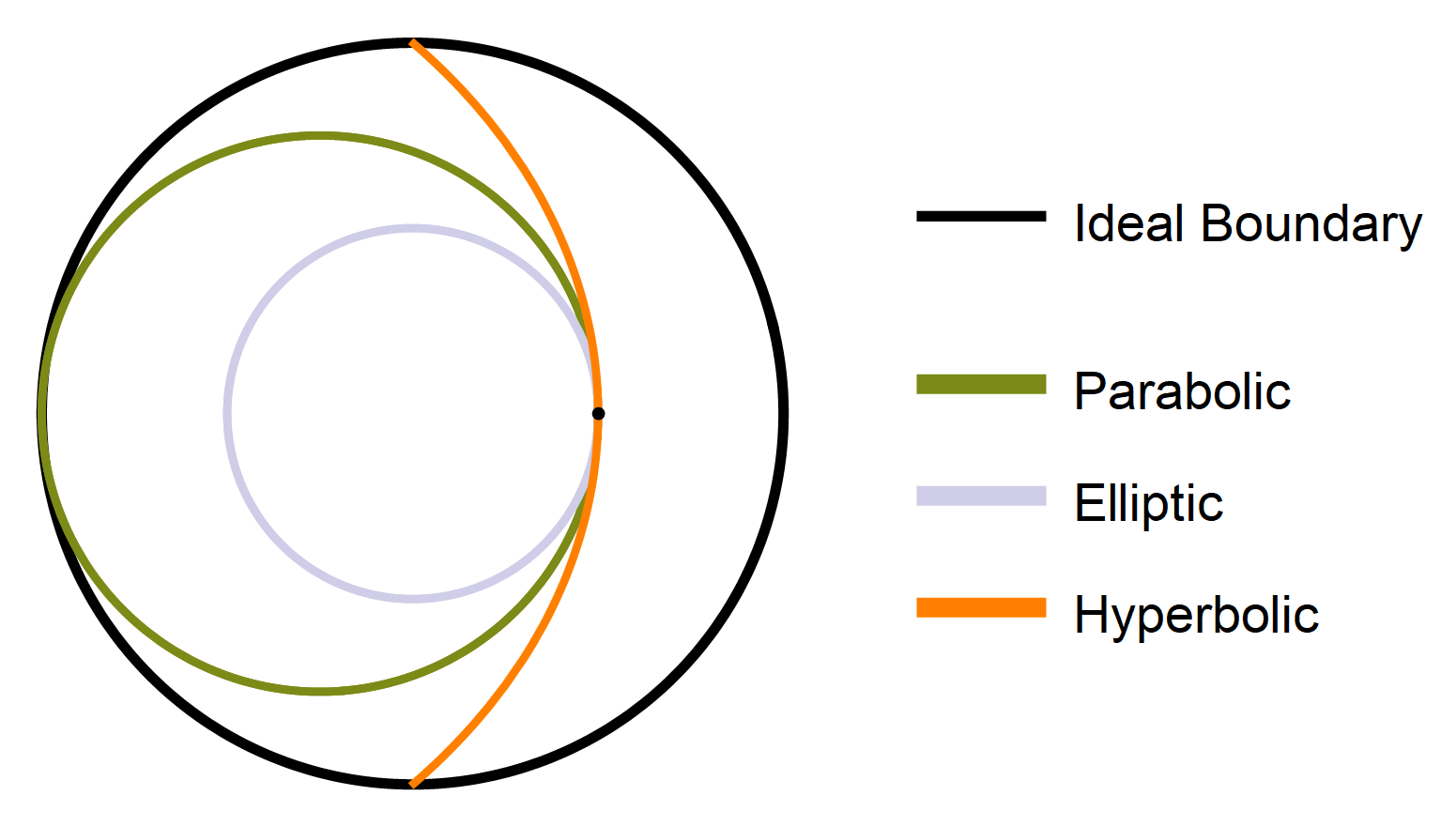
(a) Poincaré disk

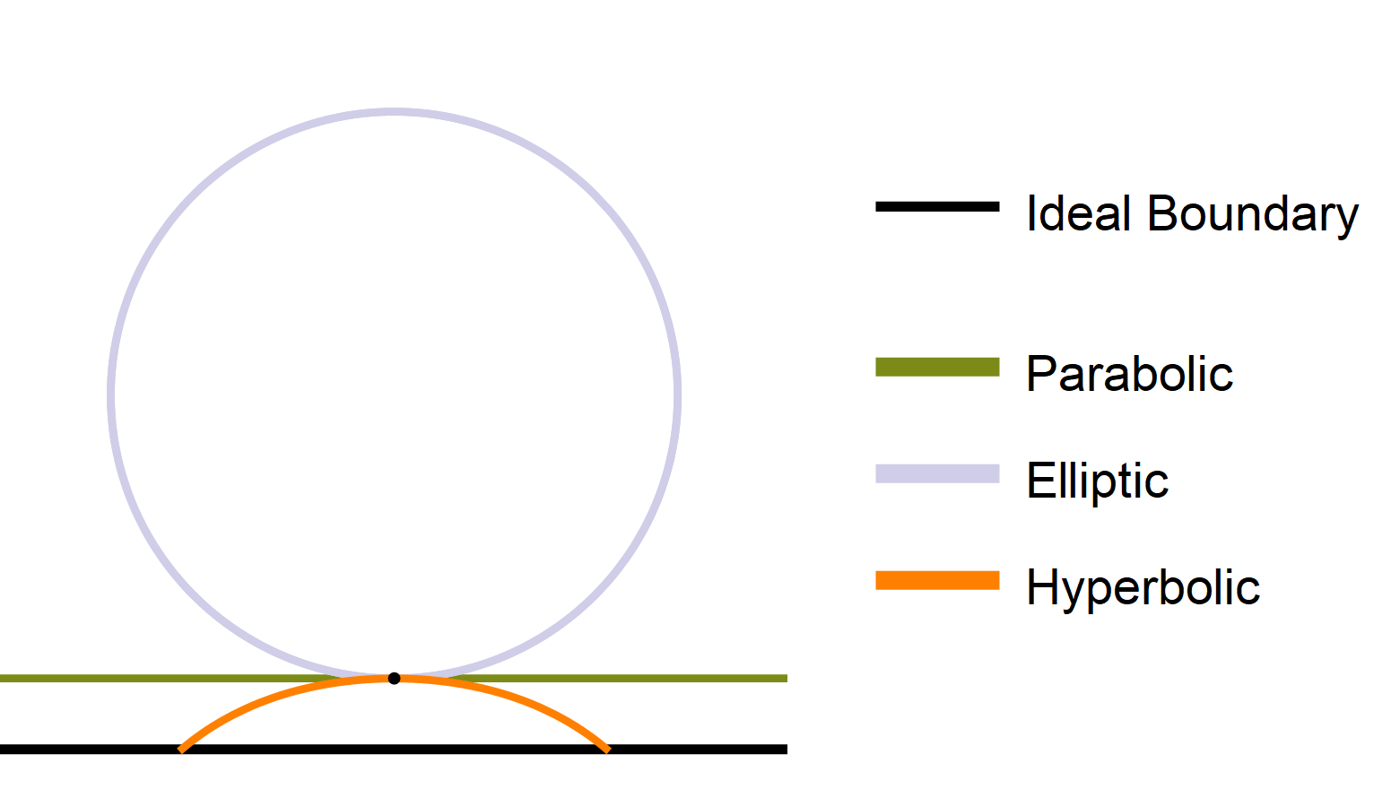
(b) Poincaré half plane

Figure 1. Visualisation of subgroups of rotation in the hyperbolic plane: The orbits of one point under all three types of subgroup of rotation are shown in the Poincaré disk and the half plane model.

We call $\mathfrak{f}:\Sigma^{2}\to\mathfrak{R}_{\mathfrak{p},\mathfrak{q}}$ a rotational surface if there is a plane $\Pi$ so that $\mathfrak{f}$ is invariant under a subgroup of rotations $\rho_{1}$ in $\Pi$. We can parametrise

$$\mathfrak{f}(t,\theta)=\rho_{1}\!\left(\theta\right)\mathfrak{c}(t),$$

with a profile curve $\mathfrak{c}=\mathfrak{f}(\cdot,0):I\to\langle\mathfrak{e}_{1}\rangle^{\perp}\cap\mathfrak{R}_{\mathfrak{p},\mathfrak{q}}$ that is orthogonal to $\mathfrak{e}_{1}$. The profile curve takes values in the sphere $\mathfrak{e}_{1}+\mathfrak{p}\in\mathfrak{T}_{\mathfrak{p},\mathfrak{q}}$, and is in this sense planar. We employ the parametrisation (5) below of rotational surfaces, see also [19, Sect 3.7.6].

We first consider the cases where $\mathfrak{v}_{1}$ is non-isotropic, hence, $\kappa_{1}\neq 0$. Let

$$\gamma(t):=\tfrac{\mathfrak{c}(t)}{\kappa_{1}r(t)},\leavevmode\nobreak\ \textrm{with}\leavevmode\nobreak\ r(t)=-\tfrac{(\mathfrak{c}(t),\mathfrak{v}_{1})}{\kappa_{1}},$$

denote the lift of the profile curve such that $(\gamma,\mathfrak{v}_{1})=-1$. Note that $r(t)$ is the $\mathfrak{v}_{1}$-coordinate function of $\mathfrak{c}$. For this new lift $\gamma$,

$$\gamma+\tfrac{1}{\kappa_{1}}\mathfrak{v}_{1}\in\Pi^{\perp},$$

is fixed by $\rho_{1}$ and we obtain the following Moutard lift of $\mathfrak{f}$:

$$\begin{split}\mathfrak{m}_{\mathfrak{f}}(t,\theta)&=\gamma(t)+\tfrac{1}{\kappa_{1}}\left(\mathfrak{v}_{1}-\rho_{1}\!\left(\theta\right)\mathfrak{v}_{1}\right)\\ &=\gamma(t)+s_{\kappa_{1}}(\theta_{1})\mathfrak{e}_{1}+\tfrac{1}{\kappa_{1}}\left(1-c_{\kappa_{1}}(\theta)\right)\mathfrak{v}_{1}.\end{split}$$ (5)

If, on the other hand, $\mathfrak{v}_{1}$ is isotropic, we choose a lightlike $\mathfrak{v}_{2}$ perpendicular to $\mathfrak{p},\mathfrak{q}$ and $\mathfrak{e}_{1}$ such that $(\mathfrak{v}_{1},\mathfrak{v}_{2})=-1$. Then we define

$$\gamma(t):=\tfrac{\mathfrak{c}(t)}{r(t)}\leavevmode\nobreak\ \textrm{with}\leavevmode\nobreak\ r(t)=-(\mathfrak{c}(t),\mathfrak{v}_{1}),$$

which yields again $(\gamma,\mathfrak{v}_{1})=-1$, but this time $r(t)$ is the $\mathfrak{v}_{2}$-coordinate function of $\mathfrak{c}(t)$. A Moutard lift of $\mathfrak{f}$ is then

$$\begin{split}\mathfrak{m}_{\mathfrak{f}}(t,\theta)&=\rho_{1}(\theta)\mathfrak{v}_{2}+\gamma(t)-\mathfrak{v}_{2}\\ &=\gamma(t)+\theta\mathfrak{e}_{1}+\tfrac{\theta^{2}}{2}\mathfrak{v}_{1}.\end{split}$$ (6)

Note that this is indeed (5) as $\tfrac{1}{\kappa_{1}}\left(1-c_{\kappa_{1}}(\theta)\right)$ converges to $\tfrac{\theta^{2}}{2}$ as $\kappa_{1}$ approaches $0$.

The tangent plane congruence $\mathfrak{t}:\Sigma^{2}\to\mathfrak{T}_{\mathfrak{p},\mathfrak{q}}$ of $\mathfrak{f}$ is also invariant under the subgroup of rotations in $\Pi$, hence also has a Moutard lift $\mathfrak{m}_{\mathfrak{t}}(t,\theta)=\rho_{1}\!\left(\theta\right)\mathfrak{v}_{1}+\nu(t)$ with a suitable $\nu:I\to\langle\mathfrak{e}_{1}\rangle^{\perp}$. As with the surface $\mathfrak{f}$, there is a function $\tilde{r}$ such that $\mathfrak{m}_{\mathfrak{t}}=\mathfrak{t}/\tilde{r}$. The conditions $(\mathfrak{m}_{\mathfrak{t}},\mathfrak{m}_{\mathfrak{f}})=(\mathfrak{m}_{\mathfrak{t}},(\mathfrak{m}_{\mathfrak{f}})_{t})=0$ and $(\mathfrak{m}_{\mathfrak{t}},\mathfrak{m}_{\mathfrak{t}})=0$ determine the map $\nu$.

The curvatures of the surface are the curvatures of its lift $\mathfrak{f}$ in $\mathbb{R}^{4,2}$ with respect to $\mathfrak{t}$, which represents the Gauss map of $\mathfrak{f}$ as a hypersurface in $\mathfrak{R}_{\mathfrak{p},\mathfrak{q}}$, as was mentioned at the beginning of Section 2.2. To obtain the Moutard lifts $\mathfrak{m}_{\mathfrak{f}}$ and $\mathfrak{m}_{\mathfrak{t}}$, we rescaled by $r$ and $\tilde{r}$ respectively, hence

$$(\mathfrak{f}_{t},\mathfrak{f}_{t})=r^{2}((\mathfrak{m}_{\mathfrak{f}})_{t},(\mathfrak{m}_{\mathfrak{f}})_{t}),\leavevmode\nobreak\ (\mathfrak{f}_{t},\mathfrak{t}_{t})=r\tilde{r}((\mathfrak{m}_{\mathfrak{f}})_{t},(\mathfrak{m}_{\mathfrak{t}})_{t}),$$ (7)

because $\mathfrak{f}$ and $\mathfrak{t}$ are lightlike. We will denote the speed of the profile curve of the Moutard lift $\mathfrak{m}_{\mathfrak{f}}$ by $v$, that is,

$$v^{2}=((\mathfrak{m}_{\mathfrak{f}})_{t},(\mathfrak{m}_{\mathfrak{f}})_{t}).$$

We proceed to provide formulas for the Gauss curvature of $\mathfrak{f}$, to be be used in Section 5. The cases where either $\kappa$ or $\kappa_{1}$ vanish need to be treated separately.

3.1. Non-isotropic cases

First assume that $\kappa_{1}\neq 0$ in a non-Euclidean space form ($\kappa\neq 0$). Then $\mathbb{R}^{4,2}$ splits as

$$\mathbb{R}^{4,2}=\langle\mathfrak{p},\mathfrak{q}\rangle\oplus_{\perp}\Pi\oplus_{\perp}\langle\mathfrak{v}_{2},\mathfrak{e}_{2}\rangle,$$

where we choose $\mathfrak{v}_{2},\mathfrak{e}_{2}\in\mathbb{R}^{4,2}$ orthogonal such that $(\mathfrak{e}_{2},\mathfrak{e}_{2})=1$ and $(\mathfrak{v}_{2},\mathfrak{v}_{2})=\kappa_{2}$ with $|\kappa_{1}|=|\kappa_{2}|$.

With suitable functions $A,B$ on $I$ and $R=\kappa_{1}/(\kappa r)$, we write

$$\mathfrak{m}_{\mathfrak{f}}(t,\theta) =\rho_{1}\!\left(\theta\right)\mathfrak{v}_{1}+R(t)\mathfrak{q}+A(t)\mathfrak{v}_{2}+B(t)\mathfrak{e}_{2},$$

$$\mathfrak{m}_{\mathfrak{t}}(t,\theta) =\rho_{1}\!\left(\theta\right)\mathfrak{v}_{1}+\tilde{R}(t)\mathfrak{p}-\tfrac{\kappa_{1}B^{\prime}(t)}{\kappa_{2}(B^{\prime}(t)A(t)-B(t)A^{\prime}(t))}\mathfrak{v}_{2}+\tfrac{\kappa_{1}A^{\prime}(t)}{B^{\prime}(t)A(t)-B(t)A^{\prime}(t)}\mathfrak{e}_{2},$$

with $\tilde{R}=1/\tilde{r}$ satisfying

$$\tilde{R}^{2}=\frac{\kappa_{1}v^{2}\kappa R^{2}}{\kappa_{2}(AB^{\prime}-A^{\prime}B)^{2}}.$$ (8)

The principal curvatures of $\mathfrak{m}_{\mathfrak{f}}$ with respect to $\mathfrak{m}_{\mathfrak{t}}$ are

$$\widetilde{k}_{1}=\frac{((\mathfrak{m}_{\mathfrak{f}})_{t},(\mathfrak{m}_{\mathfrak{t}})_{t})}{((\mathfrak{m}_{\mathfrak{f}})_{t},(\mathfrak{m}_{\mathfrak{f}})_{t})}=\kappa_{1}\frac{A^{\prime\prime}B^{\prime}-A^{\prime}B^{\prime\prime}}{v^{2}(AB^{\prime}-A^{\prime}B)},\quad\widetilde{k}_{2}=\frac{((\mathfrak{m}_{\mathfrak{f}})_{\theta},(\mathfrak{m}_{\mathfrak{t}})_{\theta})}{((\mathfrak{m}_{\mathfrak{f}})_{\theta},(\mathfrak{m}_{\mathfrak{f}})_{\theta})}=\frac{\kappa_{1}}{\kappa_{1}}=1.$$

Using (7) and (8) we obtain

$$k_{1}=\kappa_{1}\leavevmode\nobreak\ \sqrt{\frac{\kappa\kappa_{2}}{\kappa_{1}}}\leavevmode\nobreak\ \frac{A^{\prime\prime}B^{\prime}-A^{\prime}B^{\prime\prime}}{v^{3}},\quad k_{2}=\sqrt{\frac{\kappa\kappa_{2}}{\kappa_{1}}}\leavevmode\nobreak\ \frac{AB^{\prime}-A^{\prime}B}{v},$$

hence the Gauss curvature of $\mathfrak{f}$ is

$$K=\kappa\kappa_{2}\frac{(AB^{\prime}-A^{\prime}B)(A^{\prime\prime}B^{\prime}-A^{\prime}B^{\prime\prime})}{v^{4}}.$$

It is beneficial to rewrite this using polar coordinates: define $\Pi_{2}:=\langle\mathfrak{v}_{2},\mathfrak{e}_{2}\rangle$ and denote the rotation in $\Pi_{2}$ as $\rho_{2}$, analogous to $\rho_{1}$. Since $\kappa_{2}\neq 0$, we have

$$\rho_{2}\!\left(\psi\right)\mathfrak{v}_{2}=\kappa_{2}s_{\kappa_{2}}(\psi)\mathfrak{e}_{2}+c_{\kappa_{2}}(\psi)\mathfrak{v}_{2},$$

hence we write

$$A(t)\mathfrak{v}_{2}+B(t)\mathfrak{e}_{2}=D(t)\rho_{2}\!\left(\psi(t)\right)\mathfrak{v}_{2}$$

with suitable functions $D$ and $\psi$ of $t$: if $\mathfrak{v}_{2}$ is spacelike $\Pi_{2}$ is a Euclidean plane and these are the usual polar coordinates; for timelike $\mathfrak{v}_{2}$ we have $\kappa_{2}A^{2}+B^{2}=\kappa R^{2}-\kappa_{1}<0$ showing that $A\mathfrak{v}_{2}+B\mathfrak{e}_{2}$ is timelike and thus in the orbit of $D\mathfrak{v}_{2}$ for a suitably chosen function $D$. In terms of these new coordinate functions, we obtain

$$\mathfrak{m}_{\mathfrak{f}}(t,\theta)=\rho_{1}\!\left(\theta\right)\mathfrak{v}_{1}+D(t)\rho_{2}\!\left(\psi(t)\right)\mathfrak{v}_{2}+R(t)\mathfrak{q}$$ (9)

and state the following lemma:

Lemma 3.2.

For a rotational surface, given in terms of the Moutard lift (9), its Gauss curvature is given by

$$\begin{split}&K=\kappa\kappa_{2}\psi^{\prime}\leavevmode\nobreak\ \frac{\kappa\kappa_{2}D^{2}R(\psi^{\prime}R^{\prime\prime}-\psi^{\prime\prime}R^{\prime})-2\psi^{\prime}(\kappa RR^{\prime})^{2}-\psi^{\prime}(\kappa_{1}\kappa R^{\prime 2}+\kappa_{2}^{3}\psi^{\prime 2}D^{4})}{v^{4}},\\ &\textrm{with}\leavevmode\nobreak\ v^{2}=\frac{\kappa_{1}\kappa R^{\prime 2}+\kappa_{2}^{3}\psi^{\prime 2}D^{4}}{\kappa_{2}D^{2}}.\end{split}$$ (10)

Remark 3.3.

The rotations $\rho_{1}$ and $\rho_{2}$ commute, hence changing the initial value of $\psi$ results in an isometry applied to $\mathfrak{f}$ that does not change the curvature. This is reflected by the fact that only derivatives of $\psi$ appear in (10).

3.2. Isotropic cases

We now turn to the cases where either one of $\mathfrak{v}_{1}$ or $\mathfrak{q}$ is lightlike, in other words, $\mathfrak{f}$ is parabolic rotational in $\mathbb{H}^{3}$ or elliptic rotational in $\mathbb{R}^{3}$. Then, we choose $\mathfrak{v}_{2}$ lightlike such that either $(\mathfrak{v}_{1},\mathfrak{v}_{2})=-1$ or $(\mathfrak{v}_{2},\mathfrak{q})=-1$. In either case $\langle\mathfrak{v}_{1},\mathfrak{v}_{2},\mathfrak{p},\mathfrak{q}\rangle$ spans a $4$-dimensional subspace orthogonal to a spacelike plane. Let $\mathfrak{e}_{2}$ denote a vector such that $\{\mathfrak{e}_{1},\mathfrak{e}_{2}\}$ is an orthonormal basis of that plane.

3.2.1. Parabolic rotational surfaces in $\mathbb{H}^{3}$

Assume $\kappa_{1}=0$. With the notations of the previous section we obtain

$$\mathfrak{m}_{\mathfrak{f}}(t,\theta)=\rho_{1}\!\left(\theta\right)\mathfrak{v}_{2}+B(t)\mathfrak{e}_{2}+A(t)\mathfrak{v}_{1}+R(t)\mathfrak{q},$$

as the Moutard lift of $\mathfrak{f}$. The principal curvatures are

$$k_{1}=\sqrt{-\kappa}\leavevmode\nobreak\ \frac{B^{\prime}A^{\prime\prime}-B^{\prime\prime}A^{\prime}}{v^{3}},\quad k_{2}=\sqrt{-\kappa}\leavevmode\nobreak\ \frac{B^{\prime}}{v},$$

hence the Gauss curvature of $\mathfrak{f}$ is

$$K=-\kappa\frac{B^{\prime}(B^{\prime}A^{\prime\prime}-B^{\prime\prime}A^{\prime})}{v^{4}}.$$

As polar coordinates we use $\mathfrak{v}_{2}+B(t)\mathfrak{e}_{2}+A(t)\mathfrak{v}_{1}=\rho_{2}\!\left(\psi(t)\right)\mathfrak{v}_{2}+D(t)\mathfrak{v}_{1}$, where $\rho_{2}$ denotes the parabolic rotation in $\langle\mathfrak{v}_{1},\mathfrak{e}_{2}\rangle$. We arrive at the following parametrisation of the Moutard lift $\mathfrak{m}_{\mathfrak{f}}$

$$\mathfrak{m}_{\mathfrak{f}}(t,\theta)=\rho_{2}\!\left(\psi(t)\right)\rho_{1}\!\left(\theta\right)\mathfrak{v}_{2}+D(t)\mathfrak{v}_{1}+R(t)\mathfrak{q},$$ (11)

and obtain the following lemma by a straightforward computation:

Lemma 3.4.

For a rotational surface, given in terms of the Moutard lift (11), its Gauss curvature is given by

$$\begin{split}&K=\frac{\psi^{\prime}}{\kappa}\frac{\kappa R(\psi^{\prime}R^{\prime\prime}-\psi^{\prime\prime}R^{\prime})-\psi^{\prime}(\psi^{\prime 2}-\kappa R^{\prime 2})}{v^{4}},\\ &\textrm{with}\leavevmode\nobreak\ v^{2}:=((\mathfrak{m}_{\mathfrak{f}})_{t},(\mathfrak{m}_{\mathfrak{f}})_{t})=\psi^{\prime 2}-\kappa R^{\prime 2}.\end{split}$$ (12)

3.2.2. Surfaces of revolution in $\mathbb{R}^{3}$

Lastly, for $(\mathfrak{q},\mathfrak{q})=0$, we choose $\mathfrak{v}_{2}$ so that $(\mathfrak{q},\mathfrak{v}_{2})=-1$ and we may proceed similarly to the parabolic rotation case. Note, however, that in this case the roles of $A$ and $R$ are interchanged: the $\mathfrak{v}_{2}$-coefficient of the space form lift $\mathfrak{f}$ equals $1$, so $A=1/r$ if we parametrise $\mathfrak{m}_{\mathfrak{f}}$ as before. Also, $(\mathfrak{m}_{\mathfrak{t}},\mathfrak{q})=0$ translates to the $\mathfrak{v}_{2}$-part of the tangent plane congruence vanishing.

The principal curvatures are now

$$k_{1}=\sqrt{\kappa_{1}}\leavevmode\nobreak\ \frac{A^{\prime}B^{\prime\prime}-B^{\prime}A^{\prime\prime}}{v^{3}},\quad k_{2}=\frac{1}{\sqrt{\kappa_{1}}}\leavevmode\nobreak\ \frac{BA^{\prime}-AB^{\prime}}{v}.$$

The polar coordinates in $\langle\mathfrak{v}_{2},\mathfrak{e}_{2}\rangle$ are given by parabolic rotations in $\langle\mathfrak{q},\mathfrak{e}_{2}\rangle$. This results in

$$\mathfrak{m}_{\mathfrak{f}}(t,\theta)=\rho_{1}\!\left(\theta\right)\mathfrak{v}_{1}+R(t)\mathfrak{q}+D(t)\rho_{2}\!\left(\psi(t)\right)\mathfrak{v}_{2}$$ (13)

as a Moutard lift, hence $B=D\psi$ and $A=D$. We arrive at the expression for the Gauss curvature stated in the following lemma:

Lemma 3.5.

For a rotational surface, given in terms of the Moutard lift (13), the Gauss curvature is given by

$$\begin{split}&K=\frac{D^{2}\psi^{\prime}(D(\psi^{\prime}D^{\prime\prime}-\psi^{\prime\prime}D^{\prime})-2D^{\prime 2}\psi^{\prime})}{v^{4}},\\ &\textrm{with}\leavevmode\nobreak\ v^{2}=\frac{\kappa_{1}D^{\prime 2}+\psi^{\prime 2}D^{4}}{D^{2}}.\end{split}$$ (14)

4. Channel linear Weingarten surfaces

Channel surfaces can be characterised by a number of equivalent properties (see [4]). We give a definition in terms of Legendre lifts.

Definition 4.1.

A surface is called a channel surface if its Legendre lift $\Lambda$ envelops a $1$-parameter family of spheres $s$.

Remark 4.2.

Since $s$ only depends on one parameter, it is a curvature sphere congruence of $\Lambda$. Given curvature parameters $(u,v)$, there exists a lift $\mathfrak{s}$ of $s$ such that, wlog,

$$\mathfrak{s}_{v}=0.$$

Take another lift $\tilde{\mathfrak{s}}=\lambda\mathfrak{s}$ of $s$, then $\tilde{\mathfrak{s}}_{v}=\lambda_{v}\mathfrak{s}$. Thereby, a channel surface has a curvature sphere congruence $s$ such that $\mathfrak{s}_{v}\in\Gamma s$ for all lifts $\mathfrak{s}\in\Gamma s$.

Channel surfaces are examples of $\Omega_{0}$-surfaces [28]. We now consider umbilic-free channel $\Omega$-surfaces, that is, Legendre maps that are channel and have an additional $\Omega$-structure.

Let $s$ be a one parameter family of (curvature) spheres, enveloped by $\Lambda$, and denote the other curvature sphere congruence by $s_{1}$. As we stated in Proposition 2.4, the curvature sphere congruences of an $\Omega$-surface $\Lambda$ admit lifts $\mathfrak{s}_{1},\mathfrak{s}$ such that

$$(\mathfrak{s}_{1})_{u}=\phi_{u}\mathfrak{s},\quad\mathfrak{s}_{v}=\varepsilon^{2}\phi_{v}\mathfrak{s}_{1}.$$ (15)

for curvature line coordinates $(u,v)$ and $\varepsilon\in\{i,1\}$. As noted in Remark 4.2, all lifts of $s$ satisfy $\mathfrak{s}_{v}\in\Gamma s$. Together with (15) this implies $\phi_{v}=0$ and $\phi=\phi(u)$ is a function of $u$ only. Furthermore, $(\mathfrak{s}_{1})_{uv}=0$, so $\mathfrak{s}_{1}$ and $\mathfrak{s}$ are Moutard lifts of isothermic sphere congruences, as are all maps of the form

$$\mathfrak{s}_{1}+U(u)\mathfrak{s}.$$ (16)

The original version of Vessiot’s theorem [31] states that any channel isothermic surface in the conformal $3$-sphere (the space of Möbius geometry) is either a surface of revolution, a cylinder, or a cone in a suitably chosen Euclidean subgeometry. We will now prove the following Lie geometric version of this theorem.

Theorem 4.3.

A channel $\Omega$-surface is either a Dupin cyclide or a cone, a cylinder, or a surface of revolution in a suitably chosen Euclidean subgeometry,

Proof.

Let $\Pi$ denote the subspace spanned by $\mathfrak{s}$ and its $u$-derivatives. Then, because $(\mathfrak{s}_{1})_{uv}=0$, we get

$$\Pi(u)\perp\langle(\mathfrak{s}_{1})_{v},(\mathfrak{s}_{1})_{vv}\rangle=:\Pi_{1}(v).$$

Since $\Pi_{1}$ is of dimension $2$ (for non-degeneracy we assume $(\mathfrak{s}_{1})_{v}$ to be spacelike), $\Pi$ is an at most $4$-dimensional subspace of $\mathbb{R}^{4,2}$ for every $u$.

Assume $\Pi$ is $3$-dimensional at one point $u_{0}$. Then $\Pi(u_{0})^{\perp}$ is a $(2,1)$-plane in which $\mathfrak{s}_{1}$ takes its values. Thereby, $s_{1}$ is a curvature sphere congruence of a Dupin cyclide given by the splitting $\Pi(u_{0})\oplus\Pi(u_{0})^{\perp}$ (see, e.g., [28, Def 4.4]).

Now assume $\Pi$ is never $3$-dimensional. Then, because $\Pi_{1}$ only depends on $v$ and $\Pi$ only on $u$, $\Pi$ is a constant $4$-dimensional space, including at least one timelike direction. Choose any point sphere complex $\mathfrak{p}\in\Pi$ and consider the Möbius geometry modeled on $\mathfrak{p}$. After projection onto $\langle\mathfrak{p}\rangle^{\perp}$, $\Pi_{1}$ is unchanged, so the Möbius representative of $s$ moves in a $3$-space $\pi\subset\langle\mathfrak{p}\rangle^{\perp}\cong\mathbb{R}^{4,1}$. The following three cases occur (for details see [19, Sect 3.7.7]).

• If $\pi$ does not intersect the light cone $\mathcal{L}_{\mathfrak{p}}\subset\langle\mathfrak{p}\rangle^{\perp}$, then $\mathcal{L}_{\mathfrak{p}}\cap\pi^{\perp}$ contains exactly two points which are then contained in all spheres of the enveloped sphere curve $s$. Map one of these points to infinity via stereographic projection to see that the envelope is a cone.

• If $\pi$ touches $\mathcal{L}_{\mathfrak{p}}$ in one point, then all spheres of $s$ touch in precisely this point. Upon a stereographic projection, $s$ consists of planes and the envelope becomes a cylinder.

• If, finally, $\pi$ intersects $\mathcal{L}_{\mathfrak{p}}$ in two points, then $\pi^{\perp}$ consists of all spheres that share a common circle $\gamma$. Accordingly, all spheres in $s$ are perpendicular to that circle. Under a stereographic projection that maps $\gamma$ to a straight line, $s$ becomes a curvature sphere congruence of a surface of revolution.

∎

Remark 4.4.

If $\Pi$ is three-dimensional, we can choose $\mathfrak{p}$ so that $s$ consists of the spheres in an elliptic sphere pencil. Then the surface, that is, the point sphere congruence, degenerates to a circle and $s_{1}$ consists of point spheres, which furthers the analogy between Theorem 4.3 and Vessiot’s theorem: In the original theorem, it is stated that an isothermic channel surface is either rotational or its curvature lines are straight lines (i.e., the distinguished circles in the Euclidean subgeometry), whereas in Theorem 4.3 the channel $\Omega$-surface is either isothermic or the curvature spheres are points (the distinguished spheres in the Möbius subgeometry).

Now we turn to the main objects of interest for this paper: a channel linear Weingarten surface in a space form $\mathfrak{R}_{\mathfrak{p},\mathfrak{q}}$ is an $\Omega$-surface with a pair of constant conserved quantities $\mathfrak{p}^{\pm}$ spanning $\langle\mathfrak{p},\mathfrak{q}\rangle$ (see Remark 2.7) such that one curvature sphere congruence is constant along the corresponding curvature direction (recall that we assume all linear Weingarten surfaces to be non-tubular). Thus, let $\Lambda=\langle\mathfrak{s}^{+},\mathfrak{s}^{-}\rangle$ be linear Weingarten with conserved quantities $\mathfrak{p}^{\pm}$ and let $\tilde{\mathfrak{p}}\in\langle\mathfrak{p}^{+},\mathfrak{p}^{-}\rangle$ be any linear sphere complex. Consider the enveloped sphere congruence $\tilde{s}$ given by the lift

$$\tilde{\mathfrak{s}}=\mathfrak{s}_{1}-\frac{(\mathfrak{s}_{1},\tilde{\mathfrak{p}})}{(\mathfrak{s},\tilde{\mathfrak{p}})}\mathfrak{s},=\frac{1}{(\mathfrak{s},\tilde{\mathfrak{p}})}((\tilde{\mathfrak{p}},\mathfrak{s})\mathfrak{s}_{1}-(\tilde{\mathfrak{p}},\mathfrak{s}_{1})\mathfrak{s}),$$

where $s=\langle\mathfrak{s}\rangle$ is the enveloped $1$-parameter family of curvature spheres. Clearly $(\tilde{\mathfrak{s}},\tilde{\mathfrak{p}})=0$, hence $\tilde{s}$ takes values in the sphere complex $\tilde{\mathfrak{p}}$. As we saw in the proof of Proposition 2.4, the isothermic sphere congruences enveloped by $\Lambda$ are given as $\mathfrak{s}^{\pm}=\mathfrak{s}_{1}\pm\varepsilon\mathfrak{s}$ with lifts of the curvature spheres satisfying (15). Thereby we have $(\mathfrak{s}_{1},\mathfrak{p}^{\pm})=\mp\varepsilon(\mathfrak{s},\mathfrak{p}^{\pm})$, hence, $(\mathfrak{s}_{1},\mathfrak{p}^{\pm})_{v}=0$. It is now straightforward to see that $\tilde{\mathfrak{s}}_{uv}=0$, hence $\tilde{\mathfrak{s}}$ is a Moutard lift of $\tilde{s}$ (given in the form (16)). Since the plane spanned by $\mathfrak{p}^{\pm}$ is also spanned by the space form vector and the point sphere complex of the space form, we have proved the following proposition.

Proposition 4.5.

Let $\Lambda$ be a non-tubular channel linear Weingarten surface in a space form with point sphere complex $\mathfrak{p}$ and space form vector $\mathfrak{q}$. Then every sphere congruence that takes values in a linear sphere complex in $\langle\mathfrak{p},\mathfrak{q}\rangle$ is isothermic.

Corollary 4.6.

Non-tubular channel linear Weingarten surfaces in space forms (and their tangent plane congruences) are isothermic.

In Theorem 4.3, we have constructed a space form lift of a channel $\Omega$-surface in a suitably chosen Euclidean subgeometry that was invariant under a $1$-parameter family of Lie sphere transformations, namely, translations, dilations, or rotations. For channel linear Weingarten surfaces in a space form, we wish to show that these Lie sphere transformations are always rotations in the respective space form.

Theorem 4.7.

Every non-tubular channel linear Weingarten surface in a space form is a rotational surface.

Proof.

First, as stated in Remark 4.4, if $\Pi$ is $3$-dimensional at any one point then $\Lambda$ is a Dupin cyclide. However, linear Weingarten Dupin cyclides are always tubular. Thus, for a non-tubular channel linear Weingarten surface, $\Pi$ is constant and $4$-dimensional.

The sphere curve $s$ is invariant under rotations in the plane $\Pi_{1}$. Since $(\mathfrak{s}_{1})_{v}$ (hence $(\mathfrak{s}_{1})_{vv}$) is perpendicular to $\langle\mathfrak{p}^{+},\mathfrak{p}^{-}\rangle=\langle\mathfrak{p},\mathfrak{q}\rangle$, we have that $\mathfrak{p},\mathfrak{q}\perp\Pi_{1}$ and thus the rotations in $\Pi_{1}$ are indeed isometries of the considered space form. ∎

Remark 4.8.

It should be noted that the isometries that appear in the Euclidean case may be translations. However, the resulting surfaces, cylinders, are tubular. Consequently, non-tubular linear Weingarten channel surfaces in that case are always surfaces of revolution, as stated in [20, Thm 2.1].

5. Constant Gauß curvature

Let $\mathfrak{f}:\Sigma\to\mathfrak{R}_{\mathfrak{p},\mathfrak{q}}$ be a channel surface with constant Gauss curvature; then it is a rotational surface by Theorem 4.7. Let $\Pi_{1}$ denote the corresponding plane of rotations. We computed the Gauss curvature $K$ of a rotational surface in Section 3, and we will now use the fact that $K$ is constant to obtain a differential equation that determines the coordinate functions of $\mathfrak{f}$.

As in Section 3, we will also split this section into two subsections, attending to the non-isotropic and isotropic cases separately. In either subsection we will obtain a system of differential equations by choosing an appropriate parametrisation for the profile curve of the rotational surface.

5.1. Non-isotropic cases

Let $\mathfrak{f}$ be a surface of non-parabolic rotation in a non-Euclidean space form. Then $\mathbb{R}^{4,2}$ orthogonally splits into the $\mathfrak{p},\mathfrak{q}$-plane, the rotation plane $\Pi_{1}=\langle\mathfrak{v}_{1},\mathfrak{e}_{1}\rangle$ and the orthogonal complement plane $\Pi_{2}=\langle\mathfrak{v}_{2},\mathfrak{e}_{2}\rangle$. We have

$$\begin{array}[]{c|cccccc}(\leavevmode\nobreak\ ,\leavevmode\nobreak\ )&\mathfrak{p}&\mathfrak{q}&\mathfrak{v}_{1}&\mathfrak{e}_{1}&\mathfrak{v}_{2}&\mathfrak{e}_{2}\cr\hline\cr\mathfrak{p}&-1&0&0&0&0&0\cr\mathfrak{q}&0&-\kappa&0&0&0&0\cr\mathfrak{v}_{1}&0&0&\kappa_{1}&0&0&0\cr\mathfrak{e}_{1}&0&0&0&1&0&0\cr\mathfrak{v}_{2}&0&0&0&0&\kappa_{2}&0\cr\mathfrak{e}_{2}&0&0&0&0&0&1\end{array}$$ (24)

where we choose $\mathfrak{v}_{2}$ such that $|\kappa_{2}|=|\kappa_{1}|$ (note that $\kappa\kappa_{1}\kappa_{2}>0$). We denote the rotation in the plane $\Pi_{i}$ by $\rho_{i}$ and write

$$\mathfrak{f}(t,\theta)=r(t)\rho_{1}\!\left(\theta\right)\mathfrak{v}_{1}+d(t)\rho_{2}\!\left(\psi(t)\right)\mathfrak{v}_{2}+\tfrac{1}{\kappa}\mathfrak{q},$$ (25)

where we have used polar coordinates in $\Pi_{2}$. Note at this point that we are still free to chose the speed of the profile curve.

Proposition 5.1.

Let $\mathfrak{R}_{\mathfrak{p},\mathfrak{q}}$ be a non-Euclidean space form and let $\mathfrak{f}:\Sigma^{2}\to\mathfrak{R}_{\mathfrak{p},\mathfrak{q}}$ be a CGC $K\neq 0$ surface of non-parabolic rotation, parametrised as in (25).

Then, with a suitable choice of speed for the profile curve, the coordinate functions $r,\psi$ and $h$ satisfy

$$r^{\prime 2} =\tfrac{1}{\kappa\kappa_{1}\kappa_{2}}\left((1-C)+\kappa_{1}Kr^{2}\right)\left(C-\kappa_{1}(K+\kappa)r^{2}\right),$$ (26)

$$\psi^{\prime} =\tfrac{\kappa_{1}Kr^{2}+1-C}{\kappa_{2}(1-\kappa\kappa_{1}r^{2})},$$ (27)

$$d^{2} =\tfrac{1-\kappa\kappa_{1}r^{2}}{\kappa\kappa_{2}},$$ (28)

where $C$ denotes a suitable constant.

Proof.

With the Moutard lift

$$\mathfrak{m}_{\mathfrak{f}}(t,\theta)=\rho_{1}\!\left(\theta\right)\mathfrak{v}_{1}+D(t)\rho_{2}\!\left(\psi(t)\right)\mathfrak{v}_{2}+R(t)\mathfrak{q},$$

we have the following expression of the Gauss curvature in terms of $R,D$ and $\psi$

$$K=\kappa\kappa_{2}^{3}\psi^{\prime}D^{4}\leavevmode\nobreak\ \tfrac{\kappa\kappa_{2}D^{2}R(R^{\prime\prime}\psi^{\prime}-R^{\prime}\psi^{\prime\prime})-2\psi^{\prime}(\kappa RR^{\prime})^{2}}{(\kappa_{1}\kappa R^{\prime 2}+\kappa_{2}^{3}\psi^{\prime 2}D^{4})^{2}}-\tfrac{\kappa\kappa_{2}^{3}\psi^{\prime 2}D^{4}}{\kappa_{1}\kappa R^{\prime 2}+\kappa_{2}^{3}\psi^{\prime 2}D^{4}},$$ (29)

which is a simple reformulation of (10) in Lemma 3.2. We will use the fact that $K\equiv const$ to obtain a differential equation for $R=\tfrac{1}{\kappa r}$, which will then yield the differential equation for $r$.

Define

$$g(t):=\tfrac{\kappa\kappa_{1}R^{\prime 2}(t)}{\kappa\kappa_{1}R^{\prime 2}(t)+\kappa_{2}^{3}\psi^{\prime 2}(t)D^{4}(t)}.$$

Then (29) yields

$$K+\kappa=\tfrac{\kappa_{2}D^{2}R}{2\kappa_{1}R^{\prime}}(\kappa g)^{\prime}+\kappa g,$$

which implies

$$\kappa g=\tfrac{\widetilde{C}R^{2}}{\kappa_{2}D^{2}}+(K+\kappa).$$ (30)

Since $0\leq g\leq 1$, we have that

$$D^{2}\geq\tfrac{1}{\kappa\kappa_{2}}\left(\kappa_{1}K-(\kappa K+\widetilde{C})R^{2}\right)\geq 0.$$ (31)

Therefore, we obtain the elliptic differential equation

$$\kappa^{2}R^{\prime 2}=\tfrac{1}{\kappa\kappa_{1}\kappa_{2}}\left(\kappa_{1}K-(\kappa K+\widetilde{C})R^{2}\right)\left(R^{2}(\widetilde{C}+\kappa K+\kappa^{2})-\kappa_{1}(K+\kappa)\right)$$ (32)

for the function $R$ from (30) by reparameterising the $t$-coordinate so that the speed of the profile curve $\mathfrak{m}_{\mathfrak{f}}(t,0)$ (given in Lemma 3.2) satisfies

$$v^{2}=\tfrac{1}{\kappa\kappa_{2}}\left(\kappa_{1}K-(\kappa K+\widetilde{C})R^{2}\right);$$

hence setting

$$\psi^{\prime}=\tfrac{\kappa_{1}K-(\kappa K+\widetilde{C})R^{2}}{\kappa\kappa_{2}(\kappa R^{2}-\kappa_{1})},$$ (33)

without loss of generality (note that $\kappa R^{2}-\kappa_{1}=\kappa_{2}D^{2}\neq 0$). Rewriting this and (32) in terms of $r$, we obtain (26) and (27), for $C=\tfrac{1}{\kappa^{2}}(\widetilde{C}+\kappa K+\kappa^{2})$. The equation for $d$ follows from the fact that $\mathfrak{f}$ takes values in the light cone. This completes the proof. ∎

Note that the constant $C$, as defined in the last proof, satisfies

$$\tfrac{\kappa\kappa_{1}}{\kappa_{2}}(K+\kappa)r^{2}\leq\tfrac{\kappa C}{\kappa_{2}}\leq\tfrac{\kappa}{\kappa_{2}}+\tfrac{\kappa\kappa_{1}}{\kappa_{2}}Kr^{2},$$ (34)

because of (31). This imposes bounds on the sign of $C$ under certain circumstances: say $\tfrac{\kappa_{1}(K+\kappa)}{\kappa_{2}}$ is non-negative, then $\tfrac{\kappa}{\kappa_{2}}C<0$ would force $r$ to be imaginary. Similarly, if $\tfrac{\kappa_{1}\kappa K}{\kappa_{2}}$ were non-positive, $r$ would be imaginary as soon as $\tfrac{\kappa}{\kappa_{2}}(C-1)>0$. Hence, in our pursuit of real solutions, we investigate three cases:

• the intrinsic Gauss curvature $K+\kappa$ is positive and $\tfrac{\kappa}{\kappa_{2}}C\geq 0$;

• the extrinsic Gauss curvature $K$ is negative and $\tfrac{\kappa}{\kappa_{2}}(C-1)\leq 0$;

• the remaining cases, where $K+\kappa\leq 0\leq K$ and $C\in\mathbb{R}$.

The first two of these cases may overlap and the last may not occur (for instance if $\kappa=1$).

5.1.1. Positive intrinsic Gauss curvature.

We start our analysis with the assumption $K+\kappa>0$. If $C=0$ then $r\equiv 0$, hence assume $\tfrac{\kappa C}{\kappa_{2}}>0$. Then

$$y=\sqrt{\tfrac{\kappa_{1}(K+\kappa)}{C}}\leavevmode\nobreak\ r$$

is a real function and (26) takes the form

$$y^{\prime 2}=\tfrac{K+\kappa-\kappa C}{\kappa\kappa_{2}}\left(1-y^{2}\right)\left(q^{2}+p^{2}y^{2}\right)\leavevmode\nobreak\ \textrm{with}\leavevmode\nobreak\ p^{2}=\tfrac{KC}{K+\kappa-\kappa C}\leavevmode\nobreak\ \textrm{and}\leavevmode\nobreak\ p^{2}+q^{2}=1,$$

which leads to

$$y(s)=\operatorname{cn}_{p}\left(\sqrt{\tfrac{K+\kappa-\kappa C}{\kappa\kappa_{2}}}\leavevmode\nobreak\ s\right),$$

and subsequently

$$r(s)=\sqrt{\tfrac{C}{\kappa_{1}(K+\kappa)}}\leavevmode\nobreak\ \operatorname{cn}_{p}\left(\sqrt{\tfrac{K+\kappa-\kappa C}{\kappa\kappa_{2}}}\leavevmode\nobreak\ s\right),$$ (35)

where $\operatorname{cn}_{p}$ denotes a Jacobi elliptic function with modulus $p$. If $p\notin[0,1]$, a Jacobi transformation may be applied to express $r$ by another Jacobi elliptic function with modulus $\tilde{p}\in[0,1]$. For an overview of the Jacobi elliptic functions and their Jacobi transformations, see Appendix A or Section 6 for examples.

To obtain $\psi$ we need to integrate (27), which may be rewritten as

$$\psi^{\prime}(s)=-\tfrac{K}{\kappa\kappa_{2}}+\tfrac{K+\kappa}{\kappa\kappa_{2}}\left(1+\tfrac{\kappa C}{K+\kappa-\kappa C}\operatorname{sn}_{p}^{2}\left(\sqrt{\tfrac{K+\kappa-\kappa C}{\kappa\kappa_{2}}}\leavevmode\nobreak\ s\right)\right)^{-1}.$$

We can then express $\psi$ as

$$\psi(s)=-\tfrac{K}{\kappa\kappa_{2}}\leavevmode\nobreak\ s+\tfrac{K+\kappa}{\kappa\kappa_{2}}\sqrt{\tfrac{\kappa\kappa_{2}}{K+\kappa-\kappa C}}\leavevmode\nobreak\ \Pi\!\left(-\tfrac{\kappa C}{K+\kappa-\kappa C};\left.\sqrt{\tfrac{K+\kappa-\kappa C}{\kappa\kappa_{2}}}\leavevmode\nobreak\ s\right|p\right)$$ (36)

where $\Pi\!\left(k;\left.s\right|p\right)$ denotes the incomplete elliptic integral of the third kind with modulus $p$ and parameter $k$ as defined in [1, Sect 17.2], that is,

$$\Pi\!\left(k;\left.s\right|p\right)=\int_{0}^{s}\tfrac{du}{1-k\operatorname{sn}_{p}^{2}(u)}.$$

For solutions (35) with $p\notin[0,1]$, transformations of $\Pi$ can be applied (see Appendix A).

5.1.2. Negative extrinsic Gauss curvature.

Assume now that $K<0$. Then $y=\sqrt{\tfrac{\kappa_{1}K}{C-1}}r$ is real and satisfies

$$y^{\prime 2}=\tfrac{\kappa C-(K+\kappa)}{\kappa\kappa_{2}}\left(1-y^{2}\right)\left(q^{2}+p^{2}y^{2}\right)\leavevmode\nobreak\ \textrm{with}\leavevmode\nobreak\ p^{2}=\tfrac{(K+\kappa)(C-1)}{\kappa C-(K+\kappa)}\leavevmode\nobreak\ \textrm{and}\leavevmode\nobreak\ p^{2}+q^{2}=1.$$

Hence we learn that

$$r(s)=\sqrt{\tfrac{C-1}{\kappa_{1}K}}\leavevmode\nobreak\ \operatorname{cn}_{p}\left(\sqrt{\tfrac{\kappa C-(K+\kappa)}{\kappa\kappa_{2}}}\leavevmode\nobreak\ s\right).$$ (37)

Again we integrate (33) by writing

$$\psi^{\prime}(s)=-\tfrac{K}{\kappa\kappa_{2}}+\tfrac{K}{\kappa\kappa_{2}}\left(1-\tfrac{\kappa(C-1)}{\kappa C-(K+\kappa)}\operatorname{sn}_{p}^{2}\left(\sqrt{\tfrac{\kappa C-(K+\kappa)}{\kappa\kappa_{2}}}\leavevmode\nobreak\ s\right)\right)^{-1},$$

and $\psi$ is given by an incomplete integral of the third kind

$$\psi(s)=-\tfrac{K}{\kappa\kappa_{2}}\leavevmode\nobreak\ s+\tfrac{K}{\kappa\kappa_{2}}\sqrt{\tfrac{\kappa\kappa_{2}}{\kappa C-(K+\kappa)}}\leavevmode\nobreak\ \Pi\!\left(\tfrac{\kappa(C-1)}{\kappa C-(K+\kappa)};\left.\sqrt{\tfrac{\kappa C-(K+\kappa)}{\kappa\kappa_{2}}}\leavevmode\nobreak\ s\right|p\right)).$$ (38)

5.1.3. Remaining cases.

Finally, assume that $K+\kappa\leq 0\leq K$, hence $C$ a priori ranges over $\mathbb{R}$. Note that, for particular values of $C$, the solutions given in the previous two sections suffice:

• if $\tfrac{C}{\kappa_{1}}$ is negative, we can still employ the solution given in (35);

• if $\tfrac{C-1}{\kappa_{1}}$ is positive, the solution given in (37) is still real.

However, if $C$ satisfies $0\leq\tfrac{C}{\kappa_{1}}\leq\tfrac{1}{\kappa_{1}}$, both solutions are imaginary. We consider this case next. The function $y=\sqrt{\tfrac{\kappa_{1}K}{C-1}}\leavevmode\nobreak\ r$ now satisfies the differential equation

$$y^{\prime 2}=\tfrac{(-K)C}{\kappa\kappa_{2}}(1-y^{2})(1-p^{2}y^{2})\leavevmode\nobreak\ \textrm{with}\leavevmode\nobreak\ p^{2}=\tfrac{(K+\kappa)(C-1)}{KC},$$

which is solved by the Jacobi $\operatorname{sn}$ function

$$r(s)=\sqrt{\tfrac{C-1}{\kappa_{1}K}}\leavevmode\nobreak\ \operatorname{sn}_{p}\left(\sqrt{\tfrac{(-K)C}{\kappa\kappa_{2}}}\leavevmode\nobreak\ s\right).$$

To see that this is a real solution, note that the two square roots are purely imaginary. Since $\operatorname{sn}_{p}(ix)$ is imaginary, we find that $r$ is real (see Appendix A):

$$r(s) =\sqrt{\tfrac{C-1}{\kappa_{1}K}}\leavevmode\nobreak\ \operatorname{sn}_{p}\left(\sqrt{\tfrac{KC}{\kappa\kappa_{2}}}\leavevmode\nobreak\ is\right)$$

$$=-\sqrt{\tfrac{1-C}{\kappa_{1}K}}\leavevmode\nobreak\ \operatorname{sc}_{q}\left(\sqrt{\tfrac{KC}{\kappa\kappa_{2}}}\leavevmode\nobreak\ s\right),$$ (39)

wherein $q$ is defined by $p^{2}+q^{2}=1$, as usual. Note that this solution is real under our assumption $0\leq\tfrac{C}{\kappa_{1}}\leq\tfrac{1}{\kappa_{1}}$, hence in all cases where neither (35) nor (37) yield a solution.

As in the previous subsections, we may rewrite (33) as

$$\psi^{\prime}(s)=\tfrac{1-C}{\kappa_{2}}\left(1-\tfrac{K+\kappa-\kappa C}{K}\operatorname{sn}_{q}^{2}\left(\sqrt{\tfrac{KC}{\kappa\kappa_{2}}}\leavevmode\nobreak\ s\right)\right)^{-1},$$

to obtain

$$\psi(s)=\tfrac{1-C}{\kappa_{2}}\sqrt{\tfrac{\kappa\kappa_{2}}{KC}}\leavevmode\nobreak\ \Pi\!\left(\tfrac{K+\kappa-\kappa C}{K};\left.\sqrt{\tfrac{KC}{\kappa\kappa_{2}}}\leavevmode\nobreak\ s\right|q\right).$$ (40)

5.2. Isotropic scenarios

The isotropic cases are those where $\kappa$ or $\kappa_{1}$ vanishes, that is, the cases of parabolic rotational surfaces in hyperbolic space forms and of elliptic rotational surfaces in Euclidean space.

5.2.1. Parabolic rotational surfaces in $\mathbb{H}^{3}$

First, we investigate parabolic rotational surfaces in hyperbolic space: assume that $\mathfrak{v}_{1},\mathfrak{v}_{2}$ are lightlike with $(\mathfrak{v}_{1},\mathfrak{v}_{2})=-1$ and that $\mathfrak{e}_{1},\mathfrak{e}_{2}$ are unit length orthogonal vectors perpendicular to $\langle\mathfrak{v}_{1},\mathfrak{v}_{2}\rangle$ and $\langle\mathfrak{p},\mathfrak{q}\rangle$. Consider the parabolic rotations $\rho_{i}$ in $\langle\mathfrak{v}_{1},\mathfrak{e}_{i}\rangle$, which are given by

$$\rho_{i}\!\left(\theta\right):\leavevmode\nobreak\ (\mathfrak{v}_{2},\mathfrak{e}_{i},\mathfrak{v}_{1})\mapsto(\mathfrak{v}_{2}+\theta\mathfrak{e}_{i}+\tfrac{\theta^{2}}{2}\mathfrak{v}_{1},\mathfrak{e}_{i}+\theta\mathfrak{v}_{1},\mathfrak{v}_{1}).$$

Then, in polar coordinates, a parabolic rotational surface $\mathfrak{f}$ is given by

$$\mathfrak{f}(t,\theta)=\tfrac{1}{\kappa}\mathfrak{q}+r(t)\rho_{2}\!\left(\psi(t)\right)\rho_{1}\!\left(\theta\right)\mathfrak{v}_{2}+d(t)\mathfrak{v}_{1}.$$ (41)

Proposition 5.2.

Let $\mathfrak{R}_{\mathfrak{p},\mathfrak{q}}$ be a hyperbolic space form with spacelike $\mathfrak{q}$. Let $\mathfrak{f}:\Sigma^{2}\to\mathfrak{R}_{\mathfrak{p},\mathfrak{q}}$ be a CGC $K\neq 0$ parabolic rotational surface, parametrised as in (41).

Then, with a suitable choice of speed for the profile curve, the coordinate functions $r,\psi$ and $h$ satisfy

$$r^{\prime 2} =\left(-\tfrac{1}{\kappa}\right)\left(C-Kr^{2}\right)\left((K+\kappa)r^{2}-C\right),$$ (42)

$$\psi^{\prime} =\left(-\tfrac{1}{\kappa}\right)\left(K-\tfrac{C}{r^{2}}\right),$$ (43)

$$d =\left(-\tfrac{1}{\kappa}\right)\tfrac{1}{2r},$$ (44)

where $C$ denotes a suitable constant.

Proof.

Using the Moutard lift

$$\mathfrak{m}_{\mathfrak{f}}(t,\theta)=R(t)\mathfrak{q}+\rho_{2}\!\left(\psi(t)\right)\rho_{1}\!\left(\theta\right)\mathfrak{v}_{1}+D(t)\mathfrak{v}_{1},$$

we have seen in (12) that

$$K=\kappa^{2}\psi^{\prime}R\tfrac{\psi^{\prime}R^{\prime\prime}-\psi^{\prime\prime}R^{\prime}}{(\psi^{\prime 2}-\kappa R^{\prime 2})^{2}}+(-\kappa)\tfrac{\psi^{\prime 2}}{\psi^{\prime 2}-\kappa R^{\prime 2}}.$$

Similarly to the proof of Proposition 5.1, we set

$$g:=\tfrac{-\kappa R^{\prime 2}}{\psi^{\prime 2}-\kappa R^{\prime 2}}$$

to obtain

$$g=(1+\tfrac{1}{\kappa}K)+\widetilde{C}R^{2}.$$

This time, $0\leq g\leq 1$ implies

$$\tfrac{1}{\kappa}K+\widetilde{C}R^{2}\leq 0,$$

hence we derive the following differential equation for $r=\tfrac{1}{\kappa R}$:

$$r^{\prime 2}=\left(-\tfrac{1}{\kappa}\right)\left(C-Kr^{2}\right)\left((K+\kappa)r^{2}-C\right),$$

by setting $C=-\tfrac{\widetilde{C}}{\kappa}$ and choosing

$$\psi^{\prime}=v^{2}=\left(-\tfrac{1}{\kappa}\right)\left(K-\tfrac{C}{r^{2}}\right).$$ (45)

Naturally, $d$ is given by $(\mathfrak{f},\mathfrak{f})=0$, and we are done. ∎

Further, $C$ satisfies (because the function $g$ in the previous proof satisfies $0\leq g\leq 1$)

$$r^{2}(K+\kappa)\leq C\leq Kr^{2}.$$

Accordingly, for $r$ to be a real function,

• $K+\kappa>0$ dictates $C\geq 0$,

• $K<0$ dictates $C\leq 0$, whereas

• $K+\kappa\leq 0\leq K$ does not restrict $C$.

As before, we define functions $y_{1}=\sqrt{\tfrac{K+\kappa}{C}}r$ and $y_{2}=\sqrt{\tfrac{K}{C}}r$ and use them to obtain the solutions

$$\begin{split}r_{1}(s)&=\sqrt{\tfrac{C}{K+\kappa}}\operatorname{cn}_{p}\left(\sqrt{C}\leavevmode\nobreak\ s\right),\leavevmode\nobreak\ \textrm{with}\leavevmode\nobreak\ p^{2}=-\tfrac{K}{\kappa},\\ r_{2}(s)&=\sqrt{\tfrac{C}{K}}\leavevmode\nobreak\ \operatorname{cn}_{p}\left(\sqrt{-C}\leavevmode\nobreak\ s\right),\leavevmode\nobreak\ \textrm{with}\leavevmode\nobreak\ p^{2}=\tfrac{K+\kappa}{\kappa}.\end{split}$$ (46)

These solutions are real as soon as their coefficients are real (i.e., as soon as the respective $y$-function is real). This takes care of all cases: in the first two cases, the respective function provides a solution. If $K+\kappa\leq 0\leq K$, depending on the sign of $C$, one of $r_{1},r_{2}$ is real and hence a feasible solution. By (43), $\psi$ is determined as before:

$$\begin{split}\psi_{1}(s)&=-\tfrac{K}{\kappa}\leavevmode\nobreak\ s+\tfrac{K+\kappa}{\kappa\sqrt{C}}\leavevmode\nobreak\ \Pi\!\left(1;\left.\sqrt{C}\leavevmode\nobreak\ s\right|p\right),\\ \psi_{2}(s)&=-\tfrac{K}{\kappa}\leavevmode\nobreak\ s-\tfrac{K}{\kappa}\sqrt{-\tfrac{\kappa}{(K+\kappa)C}}\leavevmode\nobreak\ \Pi\!\left(p^{2};\left.\sqrt{-\tfrac{(K+\kappa)C}{\kappa}}\leavevmode\nobreak\ s\right|p\right),\end{split}$$ (47)

with an appropriate transformation applied if $p\notin[0,1]$.

5.2.2. Surfaces of revolution in $\mathbb{R}^{3}$

Finally, we consider an elliptic rotational surface in Euclidean $3$-space, i.e., a common surface of revolution. This case was fully analysed in [20], thus we just show how our setting leads to the same differential equations. Equation (14) can be rewritten as

$$\tfrac{2D^{\prime}}{D^{3}}\kappa_{1}K=g^{\prime}$$

with

$$g:=\tfrac{\kappa_{1}D^{\prime 2}}{\kappa_{1}D^{\prime 2}+\psi^{\prime 2}D^{4}}.$$

Integration of the equation then yields

$$D^{\prime 2}=\left((1-C)D^{2}+\kappa_{1}K\right)\left(CD^{2}-\kappa_{1}K\right),$$

after reparameterising the profile curve so that

$$v^{2}=\kappa_{1}\left((1-C)D^{2}+\kappa_{1}K\right).$$

In this case, we obtain the space form lift of $\mathfrak{m}_{\mathfrak{f}}$ via rescaling by $r=1/D$, and arrive (assuming $\kappa_{1}=1$) at the standard parametrisation in a suitable orthonormal basis $\{e_{1},e_{2},e_{3}\}$ of $\mathbb{R}^{3}$:

$$f(t,\theta)=r(t)\cos\theta e_{1}+r(t)\sin\theta e_{2}+\psi(t)e_{3},$$

with $r$ satisfying

$$r^{\prime 2}=\left((1-C)+Kr^{2}\right)(C-Kr^{2}),$$

which is precisely Equation (6) of [20]. Thus, for a solution, we refer the interested reader to this publication.

6. Rotational CGC surfaces in $\mathbb{S}^{3}$ and $\mathbb{H}^{3}$

In this section we discuss rotational CGC surfaces in $\mathbb{S}^{3}$ and $\mathbb{H}^{3}$, which are modelled in the classical way: consider $\mathbb{S}^{3}$ as the unit sphere in Euclidean $\mathbb{R}^{4}$ and $\mathbb{H}^{3}$ as the upper sheet of the two sheeted hyperboloid in $\mathbb{R}^{3,1}$ with the Lorentz metric. In Minkowski space $\mathbb{R}^{3,1}$, we choose the basis according to the type of rotation: for surfaces of hyperbolic and elliptic rotation, we choose an orthonormal basis, so that the metric takes the form

$$(x,y)=-x_{0}y_{0}+x_{1}y_{1}+x_{2}y_{2}+x_{3}y_{3};$$

when considering surfaces of parabolic rotation we use a pseudo-orthonormal basis and the metric is computed as

$$(x,y)=-x_{0}y_{1}-x_{1}y_{0}+x_{2}y_{2}+x_{3}y_{3}.$$

These choices result in the parametrisations for surfaces of elliptic and hyperbolic (or parabolic) rotation given in (25) (or (41)) for $|\kappa|=|\kappa_{1}|=1$ (or $\kappa=-1$) with solutions to the equations (26) and (27) (or (42) and (43)). Three different cases emerged in the solution of the differential equation satisfied by $r$. In this section, however, we want to consider the (slightly different) following three cases:

• $K$ and $K+\kappa$ are positive,

• $K$ and $K+\kappa$ are negative, and

• $K$ and $K+\kappa$ have different signs.

These arise (algebraically) from the fact that at $K=0$ and $K+\kappa=0$ the polynomial on the right side of (26) degenerates to degree $2$. This is another instance of the bifurcation that appears in the construction of constant curvature surfaces in space forms, see [16, Sect 3.2], [17] or [25] ([20] for the Euclidean case).

The boundary case $K=0$ yields tubular surfaces and is not considered in these notes. Surfaces with $K+\kappa=0$ are (intrinsically) flat. The class of intrinsically flat surfaces has been widely studied and many examples are known (e.g., the Clifford tori in $\mathbb{S}^{3}$ or the peach front in $\mathbb{H}^{3}$). We start by considering this case.

6.1. Intrinsically flat surfaces in $\mathbb{H}^{3}$ and $\mathbb{S}^{3}$

Flat surfaces of non-parabolic rotation are (mostly) a boundary case of the solution (37) to (26) given in Subsection 5.1.2:

$$r(s) =\sqrt{\tfrac{(1-C)}{\kappa_{2}}}\leavevmode\nobreak\ \operatorname{cn}_{p}\left(\sqrt{\tfrac{C}{\kappa_{2}}}\leavevmode\nobreak\ s\right)\leavevmode\nobreak\ \textrm{with}\leavevmode\nobreak\ p^{2}=\tfrac{(K+\kappa)(C-1)}{\kappa C-(K+\kappa)}$$

$$=\sqrt{\tfrac{(1-C)}{\kappa_{2}}}\leavevmode\nobreak\ \cos\left(\sqrt{\tfrac{C}{\kappa_{2}}}\leavevmode\nobreak\ s\right),$$

where we used $\operatorname{cn}_{0}=\cos$. Note that $\kappa_{2}=\kappa\kappa_{1}$ from (24). Further, from (27) we get

$$\psi(s) =s-\sqrt{\tfrac{1}{\kappa_{2}}}\leavevmode\nobreak\ \operatorname{arctan}\left(\sqrt{\tfrac{1}{C}}\leavevmode\nobreak\ \operatorname{tan}(\sqrt{\kappa_{2}C}\leavevmode\nobreak\ s)\right).$$

From (34) we then learn that

$$0\leq\kappa_{1}C\leq\kappa_{1}-\kappa\,r^{2},$$

and obtain the following results:

• For surfaces of elliptic rotation in $S^{3}$ ($\kappa=\kappa_{1}=1$), $C\in[0,1]$ which implies that $r$ and $\psi$ are real functions. For $C=1$, the surface degenerates as $r=0$. For $C=0$, however, the differential equation satisfied by $r$ degenerates to $r^{\prime}=0$, the solution to which are the Clifford tori.

• For surfaces of hyperbolic rotation in $\mathbb{H}^{3}$ ($\kappa=\kappa_{1}=-1$), $C\in[-1,0]$ is negative and $r$ as well as $\psi$ are again real (hyperbolic) functions. These surfaces are called peach fronts (see [22], [23]).

• For surfaces of elliptic rotation in $\mathbb{H}^{3}$ ($\kappa=-\kappa_{1}=-1$), $C$ is positive and

  $$r(s)=\sqrt{C-1}\leavevmode\nobreak\ \cosh\left(\sqrt{C}\leavevmode\nobreak\ s\right)$$

  is real for $C>1$, which yields snowman fronts, but is imaginary for $C<1$; in this case, we obtain as solution the real form of the solution (39):

  $$r(s) =\sqrt{1-C}\leavevmode\nobreak\ \sinh\left(\sqrt{C}\leavevmode\nobreak\ s\right),$$

  which yields an hourglass front (see [22], [23]).

For flat fronts of parabolic rotation in $\mathbb{H}^{3}$, on the other hand, we employ the parametrisation (41)

$$\mathfrak{f}(t,\theta)=-\mathfrak{q}+r(t)\rho_{2}\!\left(\psi(t)\right)\rho_{1}\!\left(\theta\right)\mathfrak{v}_{1}+d(t)\mathfrak{v}_{2},$$

with the coordinate function

$$r(s)= =\sqrt{\tfrac{C}{K}}\leavevmode\nobreak\ \operatorname{cn}_{p}\left(\sqrt{-C}\leavevmode\nobreak\ s\right),\leavevmode\nobreak\ \textrm{with}\leavevmode\nobreak\ p^{2}=1-K.$$

We see that for $K-1=0$,

$$r(s) =\sqrt{C}\leavevmode\nobreak\ \cosh(\sqrt{C}\leavevmode\nobreak\ s)$$

and integrate (43) to obtain

$$\psi(s) =s-\tfrac{\tanh(\sqrt{C}\leavevmode\nobreak\ s)}{\sqrt{C}},$$

for any $C>0$.

6.2. Rotational CGC surfaces in $\mathbb{S}^{3}$

For rotational surfaces in $\mathbb{S}^{3}$, we assume $\kappa=\kappa_{1}=\kappa_{2}=1$ in (24). In this case, (28) reduces to $d^{2}=1-r^{2}>0$, which can be used to refine (34) to yield the following cases:

• $K>0$, implying $0\leq C\leq K+1$,

• $K+1<0$, implying $K+1\leq C\leq 1$, and

• $K\in(-1,0)$, implying $0\leq C\leq 1$.

Theorem 6.2 below, combined with Proposition 2.8, then provides a complete classification of non-tubular channel linear Weingarten surfaces in $\mathbb{S}^{3}$.

Remark 6.1.

In [2] the authors consider Delaunay type surfaces, that is, rotational CMC surfaces in $\mathbb{S}^{3}$. Such surfaces are parallel to rotational surfaces of constant positive Gauss curvature. Thus explicit parametrisations of these Delaunay surfaces in a sphere can be obtained by applying a suitable parallel transformation to the parametrisations given in Theorem 6.2.

Theorem 6.2.

Every rotational constant Gauss curvature $K\neq 0$ surface in $\mathbb{S}^{3}\subset\mathbb{R}^{4}$ is given by

$$(s,\theta)\mapsto\left(r(s)\cos\theta,r(s)\sin\theta,\sqrt{1-r^{2}(s)}\leavevmode\nobreak\ \cos\psi(s),\sqrt{1-r^{2}(s)}\leavevmode\nobreak\ \sin\psi(t)\right),$$

where $r,\psi$ are listed in Table 1.

Proof.

According to Subsections 5.1.1 and 5.1.2, we obtain as potential solutions to (26)

$$r_{1}(s) =\sqrt{\tfrac{C}{K+1}}\leavevmode\nobreak\ \operatorname{cn}_{p}(\sqrt{K+1-C}\leavevmode\nobreak\ s)\leavevmode\nobreak\ \textrm{with}\leavevmode\nobreak\ p^{2}=\tfrac{KC}{K+1-C},\leavevmode\nobreak\ \textrm{or}$$

$$r_{2}(s) =\sqrt{\tfrac{C-1}{K}}\leavevmode\nobreak\ \operatorname{cn}_{p}(\sqrt{C-(K+1)}\leavevmode\nobreak\ s)\leavevmode\nobreak\ \textrm{with}\leavevmode\nobreak\ p^{2}=\tfrac{(K+1)(C-1)}{C-(K+1)}.$$

For $K>0$, the function $r_{1}$ is real and $p^{2}\in[0,\infty)$, while $r_{2}$ has an imaginary argument; this can be rectified by means of the Jacobi transformations given in Appendix A. We obtain a bifurcation of the solution space into $\operatorname{dn}$- and $\operatorname{cn}$-type solutions.

For $K+1<0$, where $r_{2}$ is real and $p^{2}\in[0,\infty)$, a similar analysis applies.

For $K\in(-1,0)$, both functions, $r_{1}$ and $r_{2}$, are real even though the arguments and $p$ may be imaginary (see Appendix A again). Writing, for example, $r_{1}$ in its real form yields

$$r_{1}(s) =\sqrt{\tfrac{C}{K+1}}\leavevmode\nobreak\ \operatorname{cd}_{p}(\sqrt{(K+1)(1-C)}\leavevmode\nobreak\ s)\leavevmode\nobreak\ \textrm{with}\leavevmode\nobreak\ p^{2}=\tfrac{(K+1)(C-1)}{KC}\leavevmode\nobreak\ \textrm{for}\leavevmode\nobreak\ C<K+1\leavevmode\nobreak\ \textrm{and}$$

$$r_{1}(s) =\sqrt{\tfrac{C}{K+1}}\leavevmode\nobreak\ \operatorname{dc}_{p}(\sqrt{(-K)C}\leavevmode\nobreak\ s)\leavevmode\nobreak\ \textrm{with}\leavevmode\nobreak\ p^{2}=\tfrac{(K+1)(C-1)}{KC}\leavevmode\nobreak\ \textrm{when}\leavevmode\nobreak\ C>K+1.$$

However, we still have the restriction $r^{2}<1$, which shows that the second form is not a feasible solution. Accordingly, we need to use the real form of $r_{2}$ in the case $C>K+1$.

Table 1 summarises the solutions, written in terms of the modulus $p$ instead of the integration constant $C$. The function $\psi$ is obtained as in Subsection 5.1.1 for each case. ∎

$K<-1$	$r(s)=\sqrt{\tfrac{p^{2}}{p^{2}-(K+1)}}\leavevmode\nobreak\ \operatorname{cn}_{p}\left(\Xi\leavevmode\nobreak\ s\right)$	$\psi(s)=\tfrac{K}{\Xi}\leavevmode\nobreak\ \Pi\!\left(\tfrac{p^{2}}{K+1};\left.\Xi\leavevmode\nobreak\ s\right|p\right)-Ks$
	$\Xi=\sqrt{\tfrac{K(K+1)}{p^{2}-(K+1)}}$,	$p\in[0,1]$
	$r(s)=\sqrt{\tfrac{1}{1-(K+1)p^{2}}}\leavevmode\nobreak\ \operatorname{dn}_{p}\left(\Xi\leavevmode\nobreak\ s\right)$	$\psi(s)=\tfrac{K}{\Xi}\leavevmode\nobreak\ \Pi\!\left(\tfrac{1}{K+1};\left.\Xi\leavevmode\nobreak\ s\right|p\right)-Ks$
	$\Xi=\sqrt{\tfrac{K(K+1)}{1-(K+1)p^{2}}}$	$p\in[0,1]$
$K=-1$	$r(s)=\sqrt{1-p^{2}}\leavevmode\nobreak\ \cos\leavevmode\nobreak\ (ps)$	$\psi(s)=s-\operatorname{arctan}\left(\tfrac{\tan(ps)}{p}\right)$
	$p\in(0,1)$
$K\in(-1,0)$	$r(s)=\sqrt{\tfrac{p^{2}}{(K+1)p^{2}-K}}\leavevmode\nobreak\ \operatorname{cd}_{p}\left(\Xi\leavevmode\nobreak\ s\right)$	$\psi(s)=\tfrac{1}{\Xi}\leavevmode\nobreak\ \Pi\!\left(\tfrac{(K+1)p^{2}}{K};\left.\Xi\leavevmode\nobreak\ s\right|p\right)$
	$\Xi=\sqrt{\tfrac{(-K)(K+1)}{(K+1)p^{2}-K}}$,	$p\in[0,1]$
	$r(s)=\sqrt{\tfrac{p^{2}}{K+1-Kp^{2}}}\leavevmode\nobreak\ \operatorname{cd}_{p}\left(\Xi\leavevmode\nobreak\ s\right)$	$\psi(s)=s-\tfrac{1}{\Xi}\leavevmode\nobreak\ \Pi\!\left(\tfrac{Kp^{2}}{K+1};\left.\Xi\leavevmode\nobreak\ s\right|p\right)$
	$\Xi=\sqrt{\tfrac{(-K)(K+1)}{K+1-Kp^{2}}}$,	$p\in[0,1]$
$K>0$	$r(s)=\sqrt{\tfrac{p^{2}}{K+p^{2}}}\leavevmode\nobreak\ \operatorname{cn}_{p}\left(\Xi\leavevmode\nobreak\ s\right)$	$\psi(s)=\tfrac{K+1}{\Xi}\leavevmode\nobreak\ \Pi\!\left(-\tfrac{p^{2}}{K};\left.\Xi\leavevmode\nobreak\ s\right|p\right)-Ks$
	$\Xi=\sqrt{\tfrac{K(K+1)}{K+p^{2}}}$,	$p\in[0,1]$
	$r(s)=\sqrt{\tfrac{1}{Kp^{2}+1}}\leavevmode\nobreak\ \operatorname{dn}_{p}\left(\Xi\leavevmode\nobreak\ s\right)$	$\psi(s)=\tfrac{K+1}{\Xi}\leavevmode\nobreak\ \Pi\!\left(-\tfrac{1}{K};\left.\Xi\leavevmode\nobreak\ s\right|p\right)-Ks$
	$\Xi=\sqrt{\tfrac{K(K+1)}{Kp^{2}+1}}$	$p\in[0,1]$

Table 1. Parameter functions of a rotational CGC surface in $\mathbb{S}^{3}$.

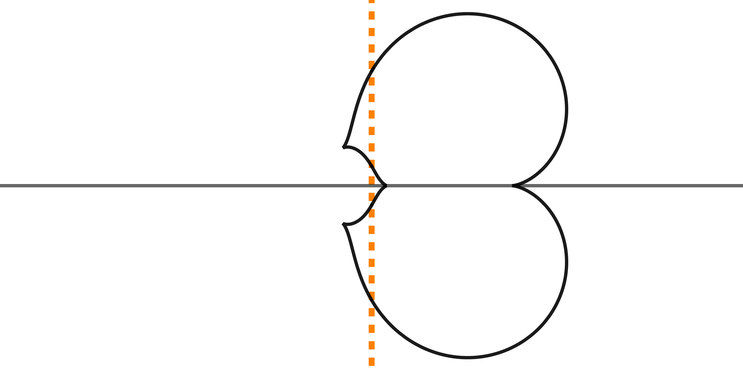
(a) $K=-2$, $\operatorname{cn}$-type

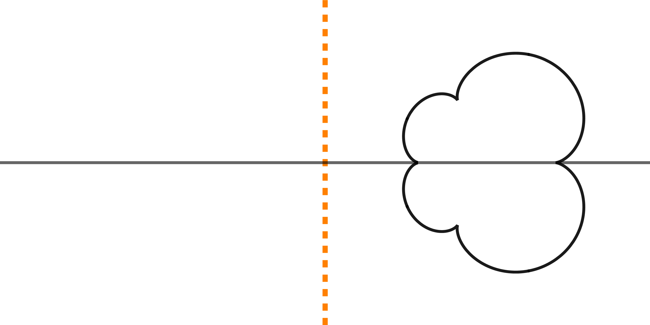
(b) $K=-2$, $\operatorname{dn}$-solution

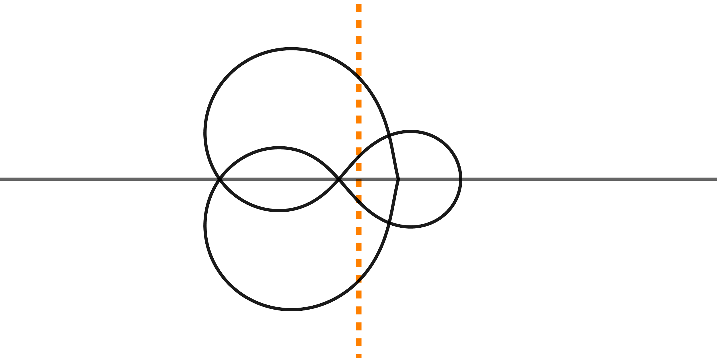
(c) $K=-0.4$,first $\operatorname{cd}$-solution

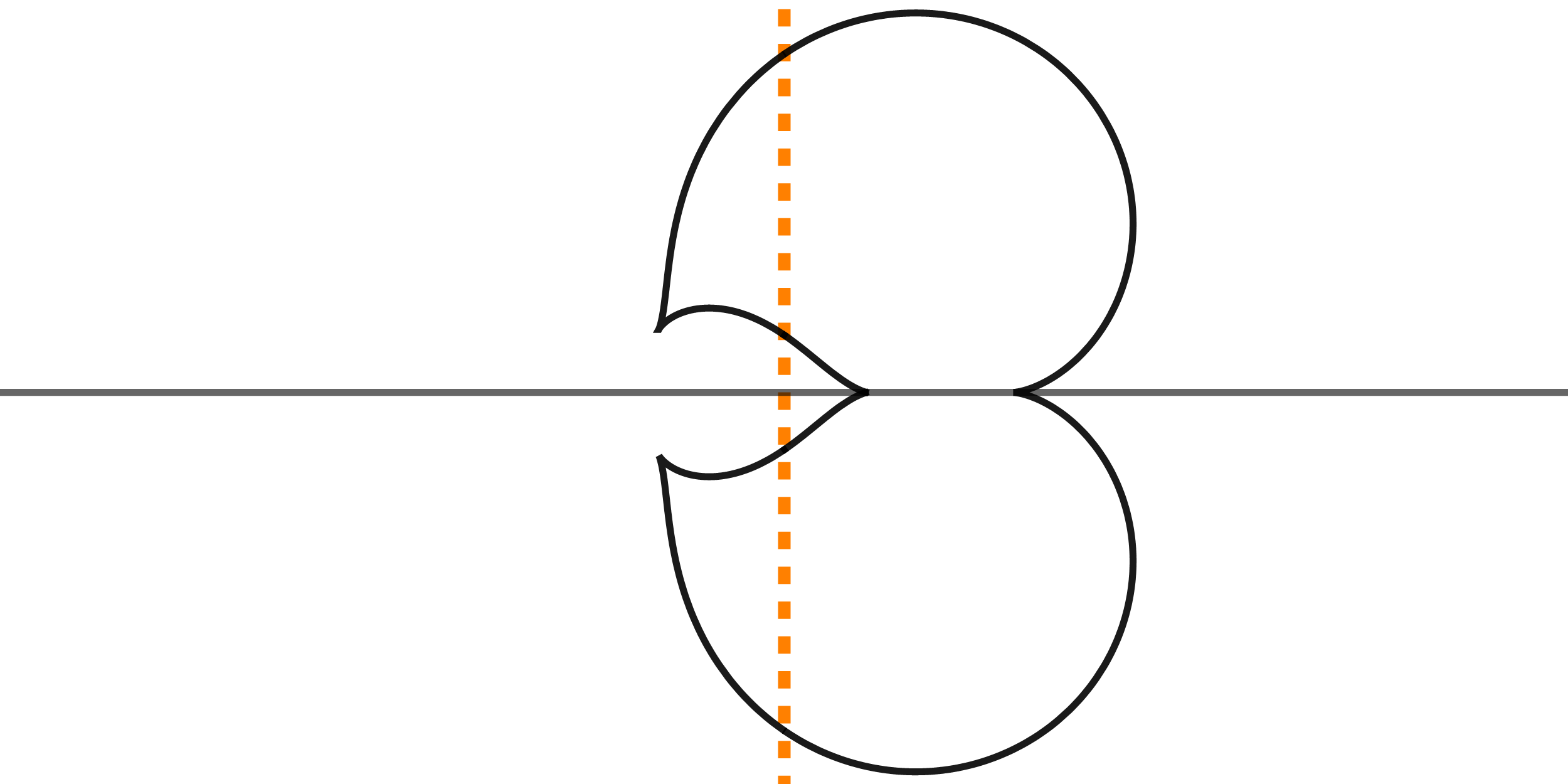
(d) $K=-0.4$, second $\operatorname{cd}$-solution

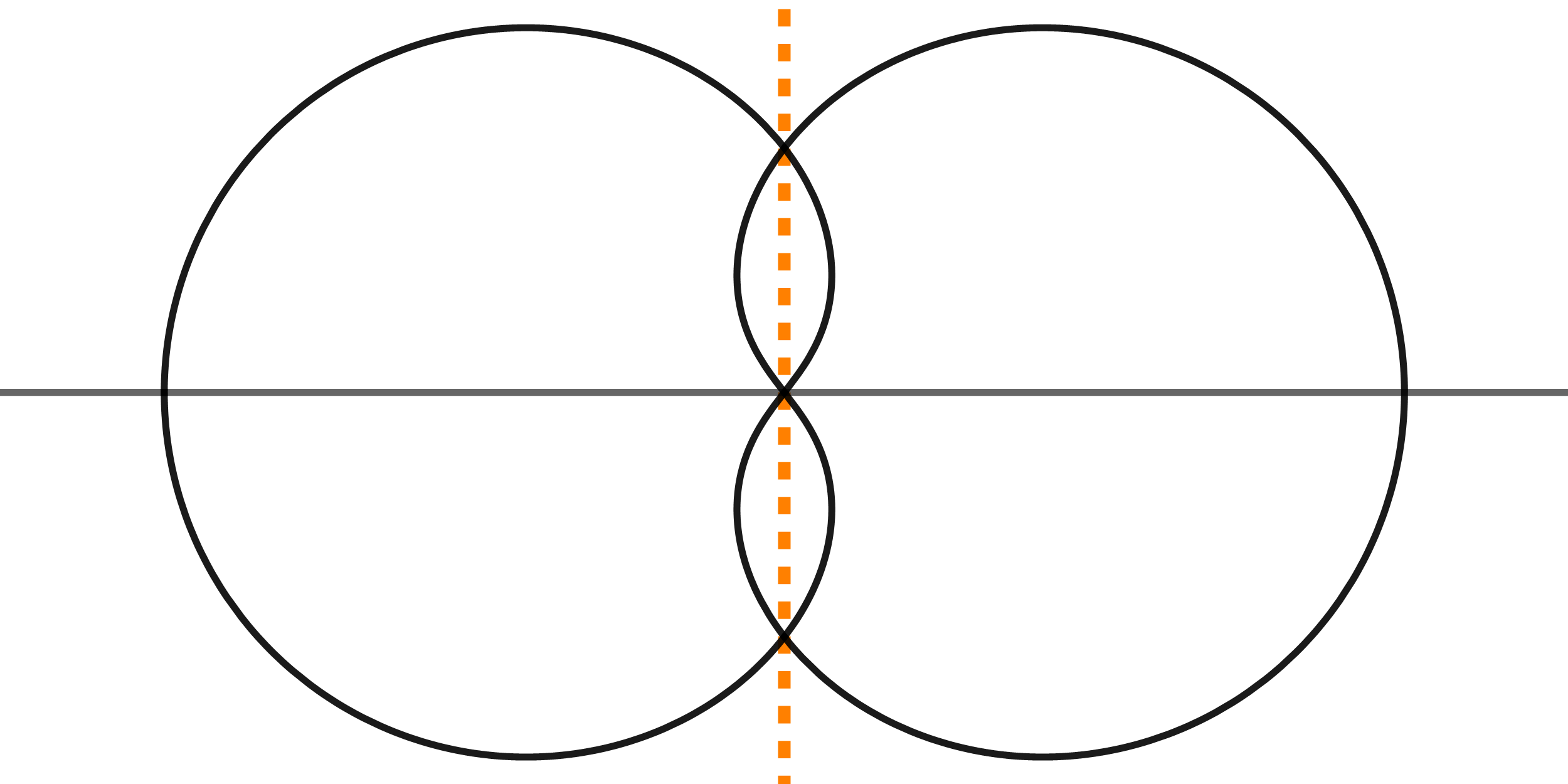
(e) $K=1$, $\operatorname{cn}$-solution

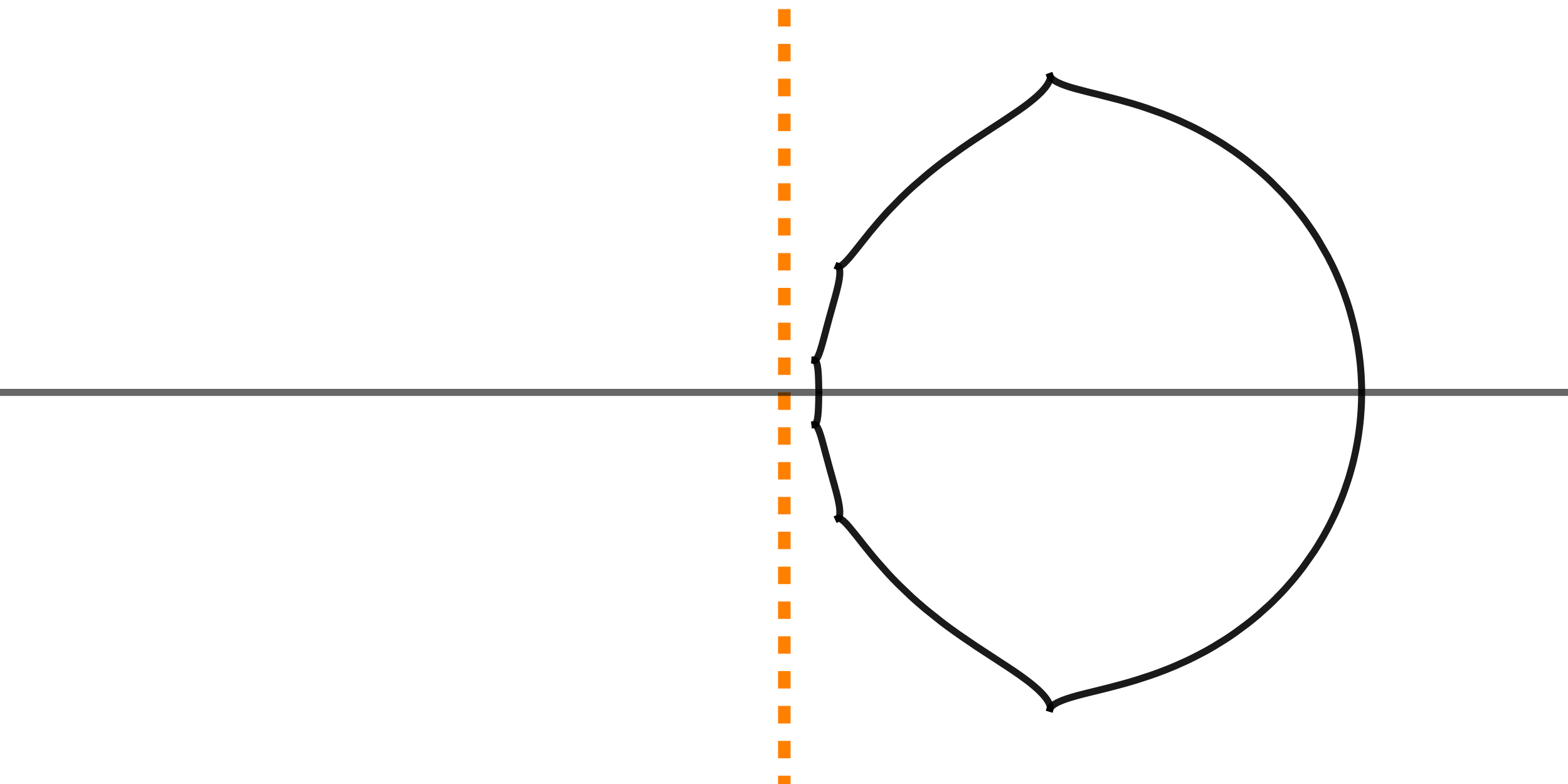
(f) $K=1$, $\operatorname{dn}$-solution

Figure 2. Profile curves of CGC surfaces of elliptic rotation in $\mathbb{S}^{3}$ after stereographic projection: the dashed line represents the axis of rotation. The profile curves are obtained from the solutions in Table 1 and the surfaces obtained via rotation are displayed in Figure 3.

(a) $K=-2$, $\operatorname{cn}$-solution

(b) $K=-2$, $\operatorname{dn}$-solution

(c) $K=-0.4$, first solution

(d) $K=-0.4$, second solution

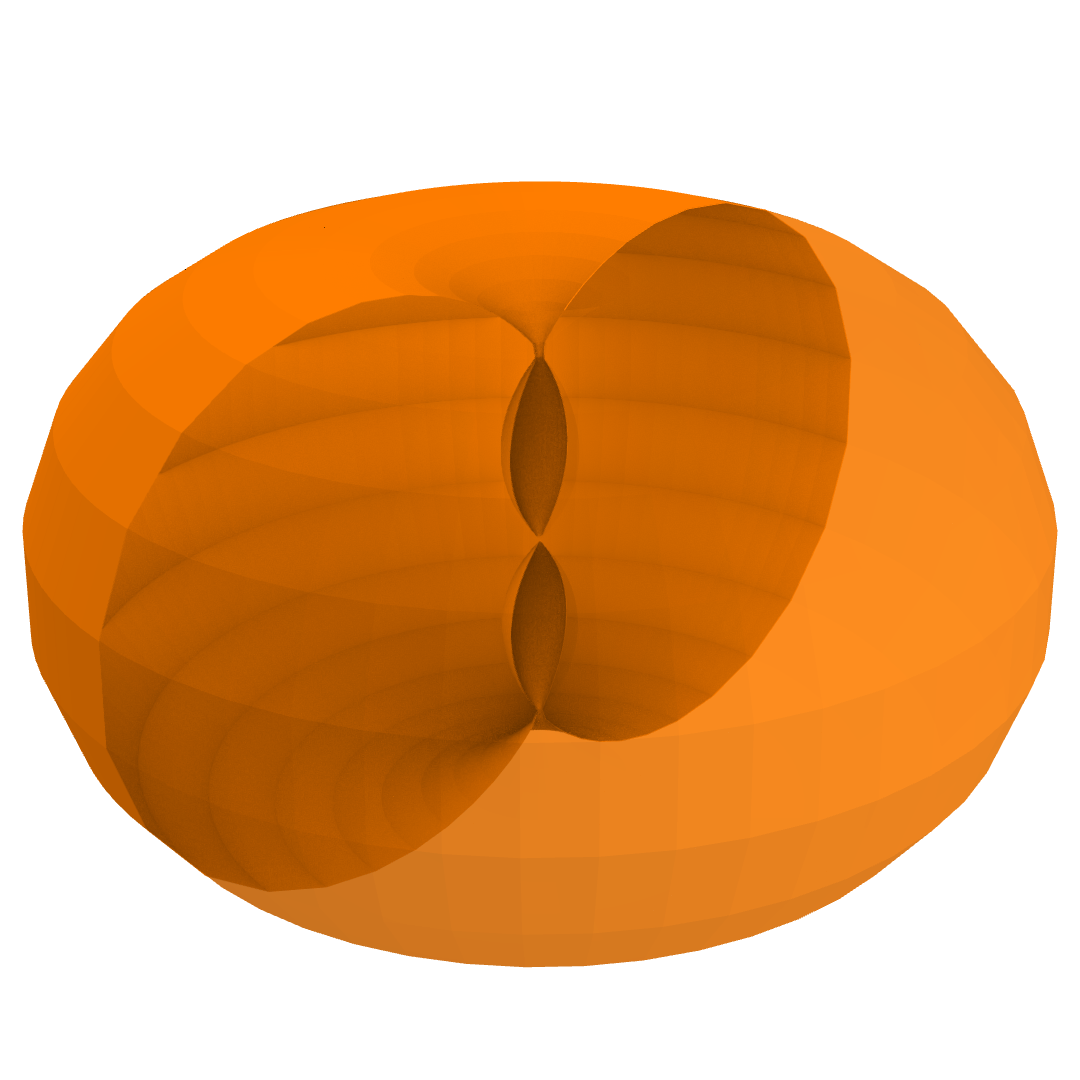
(e) $K=1$, $\operatorname{cn}$-solution

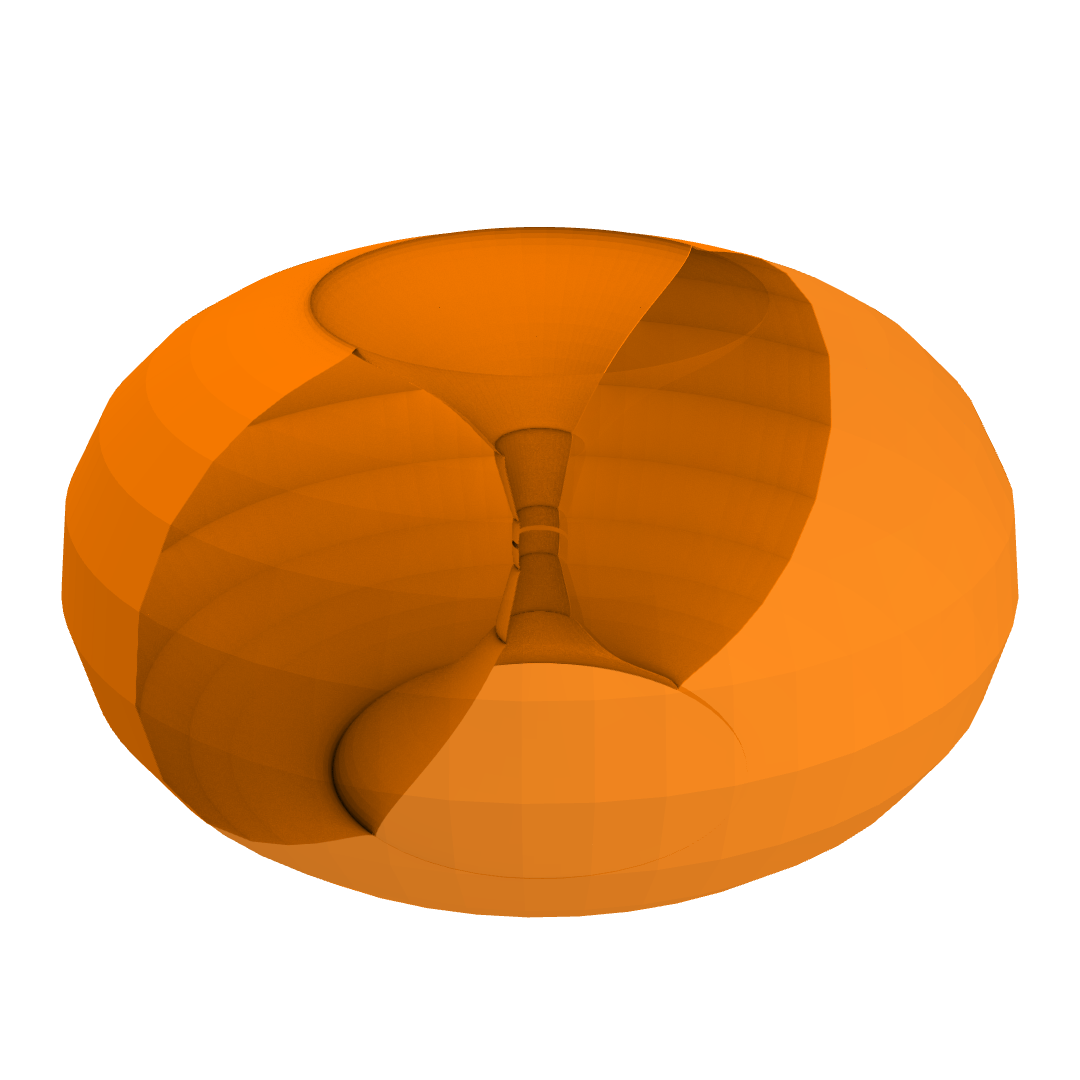
(f) $K=1$, $\operatorname{dn}$-solution

Figure 3. Stereographic projections of rotational surfaces of different Gauss curvatures in $\mathbb{S}^{3}$. The figures are obtained from the parametrisation given in Theorem 6.2, with the functions $r$ and $\psi$ from Table 1; the meridian curves are shown in Figure 2.

6.3. CGC surfaces of elliptic rotation in $\mathbb{H}^{3}$

For surfaces of elliptic rotation in $\mathbb{H}^{3}$, we assume ${\kappa_{1}=-\kappa_{2}=1}$ and $\kappa=-1$ in (24), which amounts to choosing an orthonormal basis in the $4$-dimensional space ${\{v\in\mathbb{R}^{4,2}|(v,\mathfrak{q})=-1,\leavevmode\nobreak\ (v,\mathfrak{p})=0\}}$, viewed as a copy of $\mathbb{R}^{3,1}$. In this case (28) reads $d^{2}=r^{2}+1$ which poses no additional condition. Thus (34) yields the cases

• $K-1>0$ with $C>0$,

• $K<0$ with $C-1<0$ and

• $K\in(0,1)$ with $C$ unrestricted.

By Proposition 2.8, every linear Weingarten surface with $\left|\tfrac{a+c}{2}\right|>|b|$ is parallel to a CGC surface with $K\neq 0$. On the other hand, if $ac-b^{2}<0$, then its parallel family also contains a pair of constant mean curvature $H>1$ or constant harmonic mean curvature surfaces $K/H<1$.

Constant mean curvature $H$ surfaces of elliptic rotation are considered in [18]. In the case $H>1$, these arise in $1$-parameter families that are similar to that of Delaunay surfaces in $\mathbb{R}^{3}$. By Proposition 2.8, these surfaces are parallel to the CGC surfaces considered here.

Theorem 6.3.

Every constant Gauss curvature $K\neq 0$ surface of elliptic rotation in $\mathbb{H}^{3}\subset\mathbb{R}^{3,1}$ is given in an orthonormal basis by

$$(s,\theta)\mapsto\left(\sqrt{1+r^{2}(s)}\leavevmode\nobreak\ \cosh\psi(s),\sqrt{1+r^{2}(s)}\leavevmode\nobreak\ \sinh\psi(s),r(s)\cos\theta,r(s)\sin\theta\right),$$

where $r$, $\psi$ are listed in Table 2.

$K<0$	$r(s)=\sqrt{\frac{p^{2}}{1-K-p^{2}}}\leavevmode\nobreak\ \operatorname{cn}_{p}\left(\Xi\leavevmode\nobreak\ s\right)$	$\psi(s)=\tfrac{K}{\Xi}\leavevmode\nobreak\ \Pi\!\left(\frac{p^{2}}{1-K};\left.\Xi\leavevmode\nobreak\ s\right|p\right)-Ks$
	$\Xi=\sqrt{\frac{(-K)(1-K)}{1-K-p^{2}}}$,	$p\in[0,1]$
	$r(s)=\sqrt{\frac{1}{(1-K)p^{2}-1}}\leavevmode\nobreak\ \operatorname{dn}_{p}\left(\Xi\leavevmode\nobreak\ s\right)$	$\psi(s)=\tfrac{K}{\Xi}\leavevmode\nobreak\ \Pi\!\left(\frac{1}{1-K};\left.\Xi\leavevmode\nobreak\ s\right|p\right)-Ks$
	$\Xi=\sqrt{\frac{(-K)(1-K)}{(1-K)p^{2}-1}}$,	$p\in\left[\sqrt{\frac{1}{1-K}},1\right]$
$K\in(0,1)$	$r(s)=\sqrt{\frac{1-p^{2}}{K-1+p^{2}}}\leavevmode\nobreak\ \operatorname{nc}_{p}\left(\Xi\leavevmode\nobreak\ s\right)$	$\psi(s)=\tfrac{\Xi(1-p^{2})}{K}\leavevmode\nobreak\ \Pi\!\left(\tfrac{1-K}{\Xi^{2}};\left.\Xi\leavevmode\nobreak\ s\right|p\right)-\tfrac{\Xi^{2}p^{2}}{1-K}s$
	$\Xi=\sqrt{\frac{K(1-K)}{K-1+p^{2}}}$,	$p\in[\sqrt{1-K},1]$
	$r(s)=\sqrt{\frac{1-p^{2}}{1+p^{2}(K-1)}}\leavevmode\nobreak\ \operatorname{sc}_{p}\left(\Xi\leavevmode\nobreak\ s\right)$	$\psi(s)=\tfrac{\Xi(1-p^{2})}{K}\leavevmode\nobreak\ \Pi\!\left(\tfrac{\Xi^{2}p^{2}}{1-K};\left.\Xi\leavevmode\nobreak\ s\right|p\right)-s$
	$\Xi=\sqrt{\frac{K(1-K)}{1+p^{2}(K-1)}}$,	$p\in[0,1]$
	$r(s)=\sqrt{\frac{1-p^{2}}{1-Kp^{2}}}\leavevmode\nobreak\ \operatorname{sc}_{p}\left(\Xi\leavevmode\nobreak\ s\right)$	$\psi(s)=\tfrac{\Xi(1-p^{2})}{K-1}\leavevmode\nobreak\ \Pi\!\left(\tfrac{\Xi^{2}p^{2}}{K};\left.\Xi\leavevmode\nobreak\ s\right|p\right)$
	$\Xi=\sqrt{\frac{K(1-K)}{1-Kp^{2}}}$,	$p\in[0,1]$
	$r(s)=\sqrt{\frac{1-p^{2}}{p^{2}-K}}\leavevmode\nobreak\ \operatorname{nc}_{p}\left(\Xi\leavevmode\nobreak\ s\right)$	$\psi(s)=\tfrac{\Xi(1-p^{2})}{K-1}\leavevmode\nobreak\ \Pi\!\left(\tfrac{K}{\Xi^{2}};\left.\Xi\leavevmode\nobreak\ s\right|p\right)+\tfrac{\Xi^{2}(1-p^{2})}{1-K}s$
	$\Xi=\sqrt{\frac{K(1-K)}{p^{2}-K}}$,	$p\in[\sqrt{K},1]$
$K=1$	$r(s)=\sqrt{\tfrac{1-p^{2}}{p^{2}}}\leavevmode\nobreak\ \cosh\leavevmode\nobreak\ \left(\tfrac{s}{p}\right)$	$\psi(s)=s-\operatorname{artanh}\left(p\tanh\left(\tfrac{s}{p}\right)\right)$
	$p\in(0,1)$	Snowman fronts
	$r(s)=\sqrt{1-p^{2}}\leavevmode\nobreak\ \sinh\leavevmode\nobreak\ (ps)$	$\psi(s)=\tfrac{1}{1-p^{2}}\left(s-\operatorname{artanh}(p\leavevmode\nobreak\ \tanh(ps)\right)$
	$p\in(0,1)$	Hourglass fronts
$K>1$	$r(s)=\sqrt{\frac{p^{2}}{K-p^{2}}}\leavevmode\nobreak\ \operatorname{cn}_{p}\left(\Xi\leavevmode\nobreak\ s\right)$	$\psi(s)=\tfrac{K-1}{\Xi}\leavevmode\nobreak\ \Pi\!\left(\frac{p^{2}}{K};\left.\Xi\leavevmode\nobreak\ s\right|p\right)-Ks$
	$\Xi=\sqrt{\frac{K(K-1)}{K-p^{2}}}$,	$p\in[0,1]$
	$r(s)=\sqrt{\frac{1}{Kp^{2}-1}}\leavevmode\nobreak\ \operatorname{dn}_{p}\left(\Xi\leavevmode\nobreak\ s\right)$	$\psi(s)=\tfrac{K-1}{\Xi}\leavevmode\nobreak\ \Pi\!\left(\frac{1}{K};\left.\Xi\leavevmode\nobreak\ s\right|p\right)-Ks$
	$\Xi=\sqrt{\frac{K(K-1)}{Kp^{2}-1}}$,	$p\in\left[\sqrt{\frac{1}{K}},1\right]$

Table 2. Parameter functions of CGC surfaces of elliptic rotation in $\mathbb{H}^{3}$.

Remark 6.4.

The bifurcation in the mixed case $K\in(0,1)$ is of a slightly different flavor than before. Since $C$ is unbounded, three cases emerge: for $C<0$ the solution of Subsection 5.1.1 is real with $p>1$ and imaginary argument, which yields an $\operatorname{nc}$-type solution. Similarly, for $C>1$, the solution of Subsection 5.1.2 takes an $\operatorname{nc}$-form. If, however, $C\in[0,1]$ the solution to (26) is given in Subsection 5.1.3, with $p^{2}\in[0,\infty)$ which splits again in two cases with moduli in $[0,1]$, which yields the $\operatorname{sc}$-type solutions.

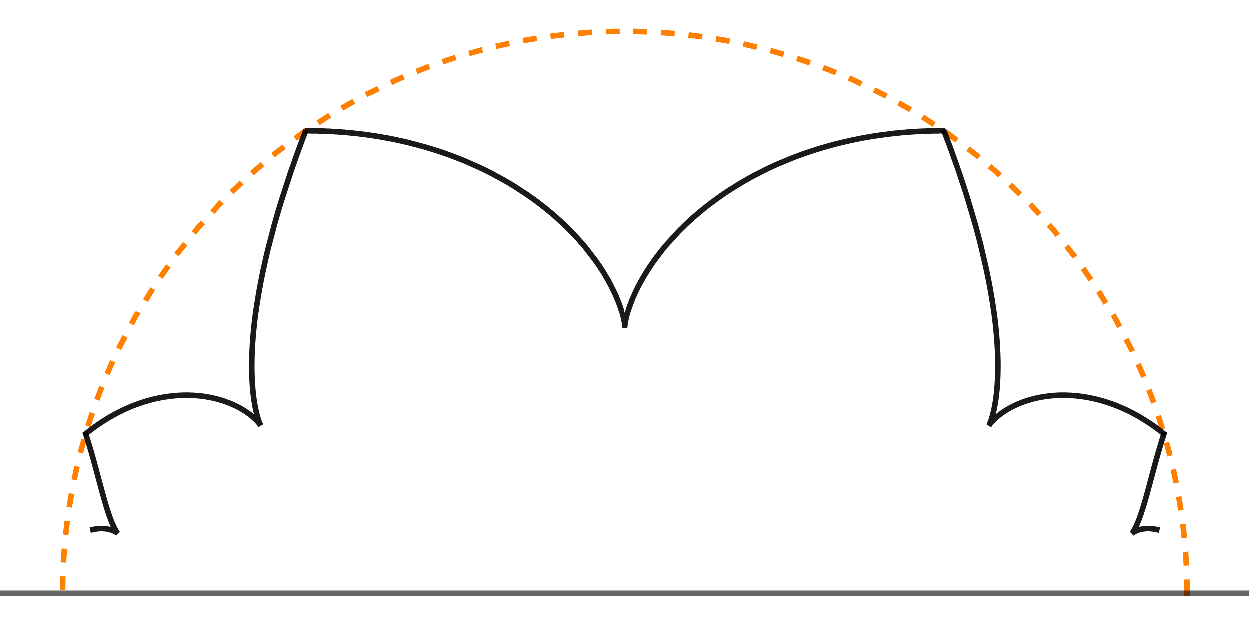
(a) $K=-1$, $\operatorname{cn}$-solution

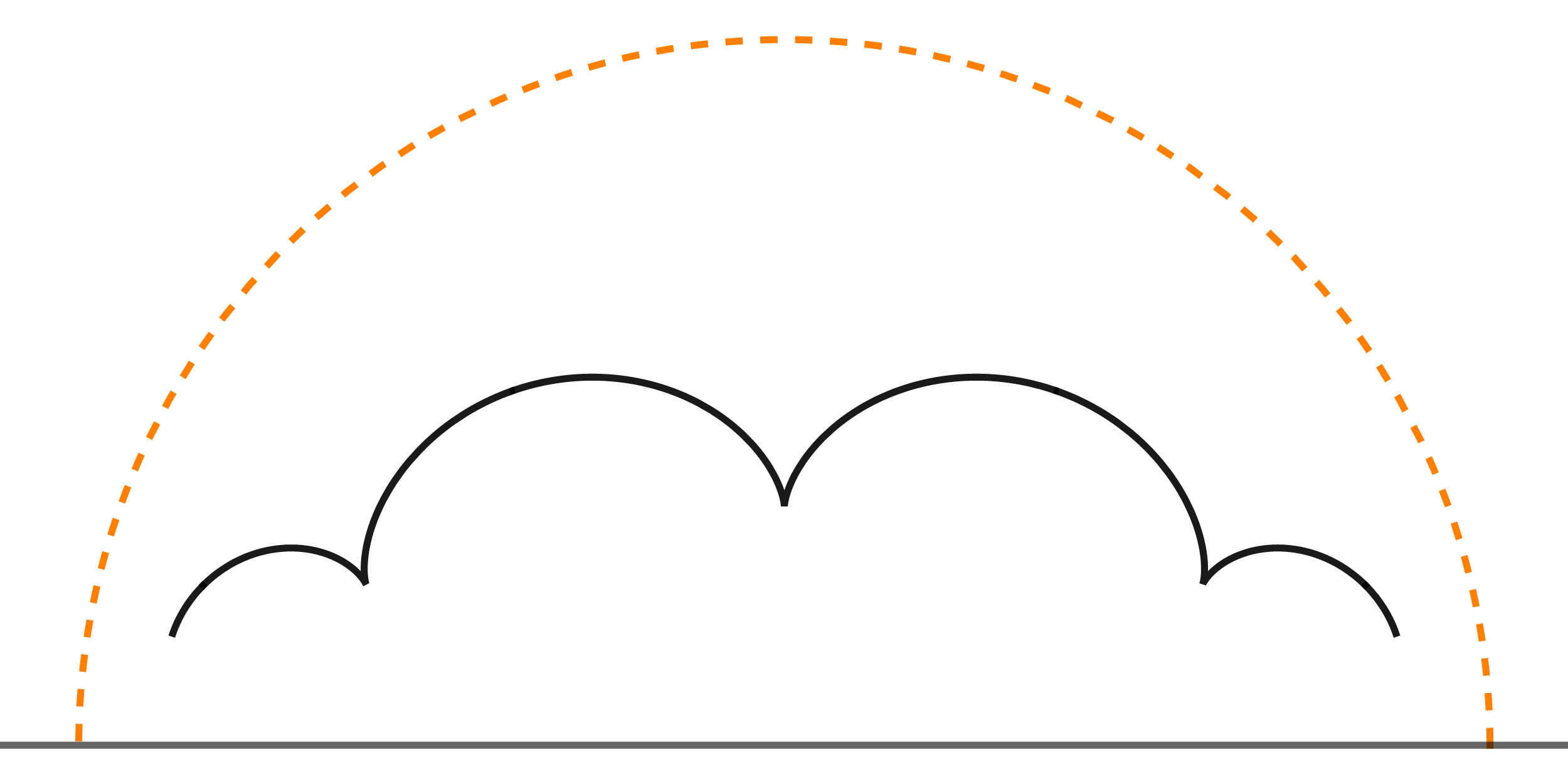
(b) $K=-1$, $\operatorname{dn}$-solution

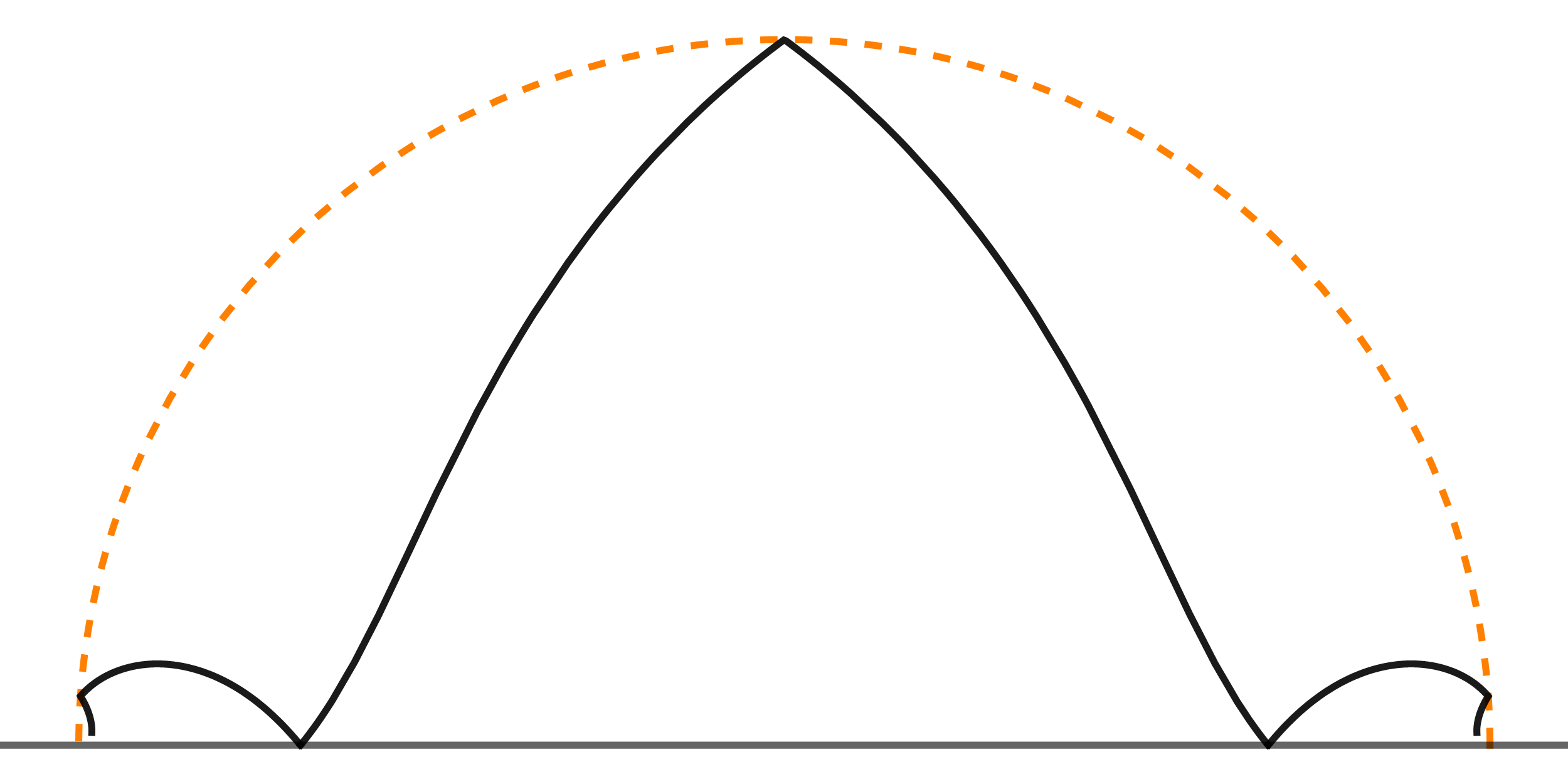
(c) $K=0.4$, first $\operatorname{sc}$-solution

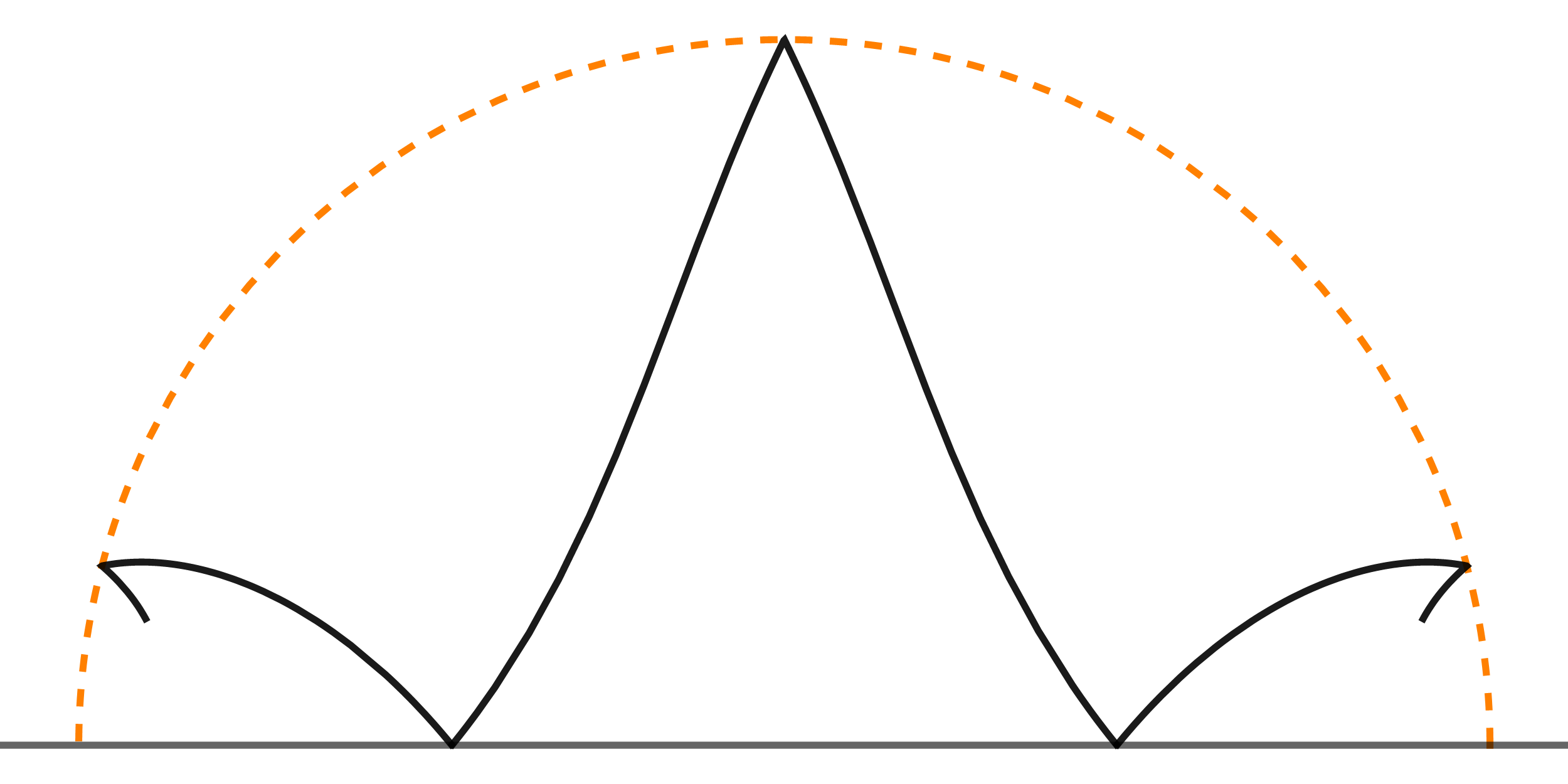
(d) $K=0.4$, second $\operatorname{sc}$-solution

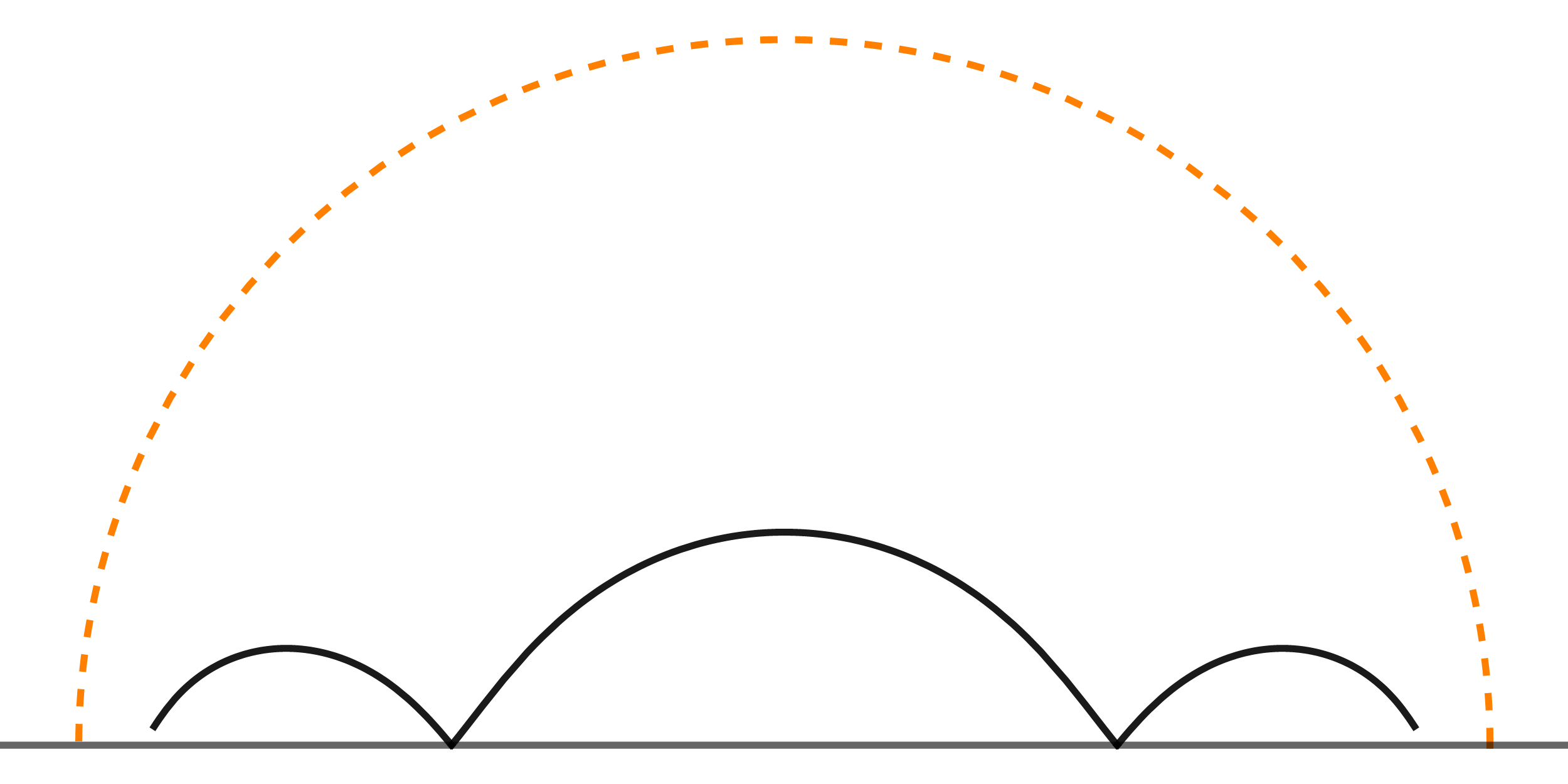
(e) $K=0.4$, first $\operatorname{nc}$-solution

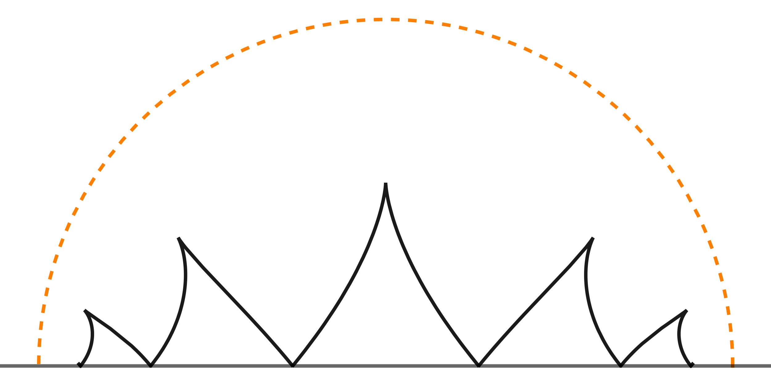
(f) $K=0.4$, second $\operatorname{nc}$-solution

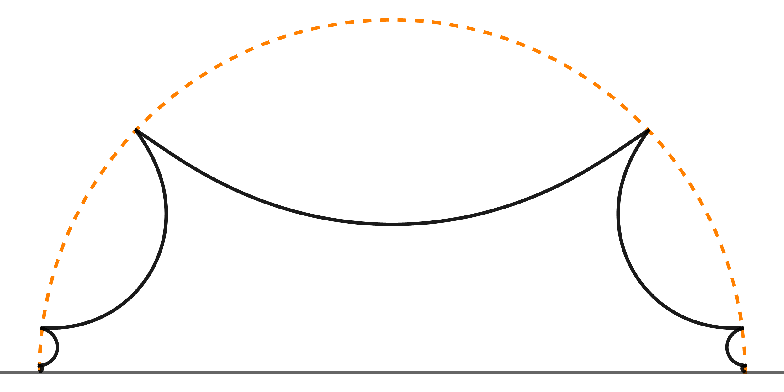
(g) $K=2$, $\operatorname{cn}$-solution

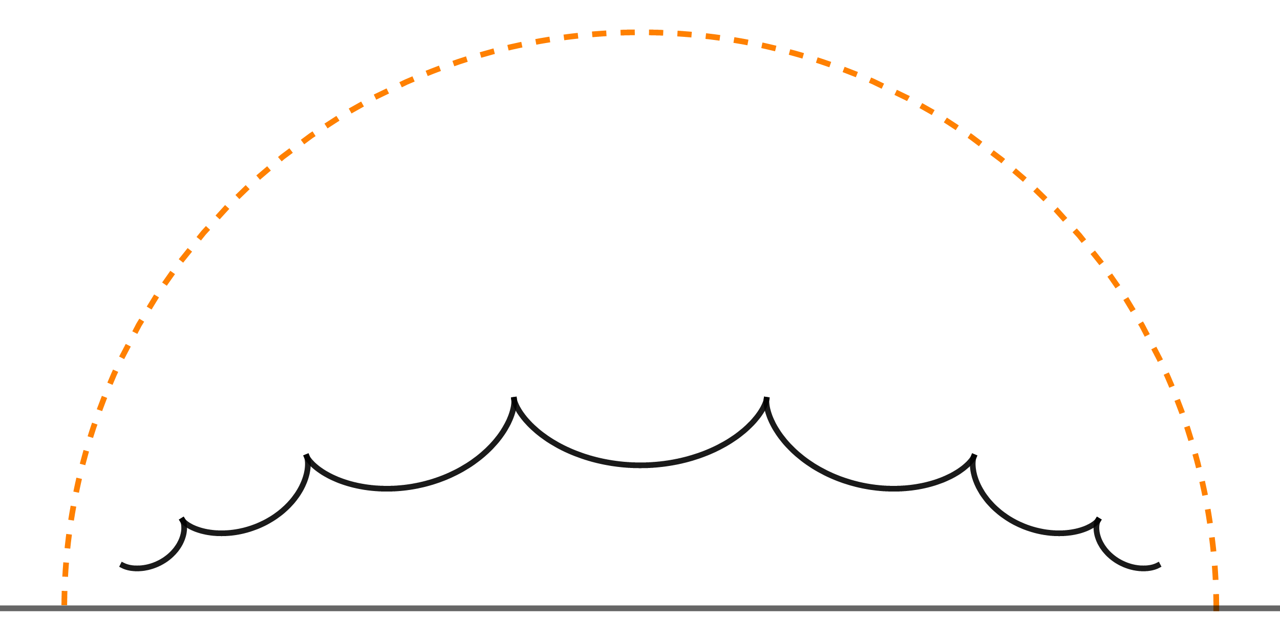
(h) $K=2$, $\operatorname{dn}$-solution

Figure 4. Profile curves of CGC surfaces of elliptic rotation in the half plane model: the dashed line represents the axis of rotation. The profile curves are obtained using the solutions in Table 2. The elliptic rotational surfaces corresponding to the profile curves in Figures 4(a), 4(c) and 4(g) are displayed in Figures 8(a), 8(b) and 8(c), respectively.

6.4. CGC surfaces of hyperbolic rotation in $\mathbb{H}^{3}$

For surfaces of hyperbolic rotation we assume $\kappa_{1}=-\kappa_{2}=-1$ and, as before, $\kappa=-1$ in (24). In this case, because $d^{2}=r^{2}-1$ according to (28), we are restricted to solutions of (26) with $r^{2}>1$. Thus (34) yields the three cases

• $K-1>0$, which implies $-C>K-1$,

• $K<0$, implying $-C<K-1$, and

• $K\in(0,1)$ with $C$ unrestricted.

Theorem 6.5.

Every constant Gauss curvature $K\neq 0$ surface of hyperbolic rotation in $\mathbb{H}^{3}\subset\mathbb{R}^{3,1}$ is given in an orthonormal basis by

$$(s,\theta)\mapsto\left(r(s)\cosh\theta,r(s)\sinh\theta,\sqrt{r^{2}(s)-1}\leavevmode\nobreak\ \cos\psi(s),\sqrt{r^{2}(s)-1}\leavevmode\nobreak\ \sin\psi(s)\right),$$

where $r$, $\psi$ are listed in Table 3.

$K<0$	$r(s)=\sqrt{\frac{1}{1+(K-1)p^{2}}}\leavevmode\nobreak\ \operatorname{dn}_{p}\left(\Xi\leavevmode\nobreak\ s\right)$	$\psi(s)=\tfrac{K}{\Xi}\leavevmode\nobreak\ \Pi\!\left(\frac{1}{1-K};\left.\Xi\leavevmode\nobreak\ s\right|p\right)-Ks$
	$\Xi=\sqrt{\tfrac{K(K-1)}{1+(K-1)p^{2}}}$,	$p\in\left[0,\sqrt{\frac{1}{1-K}}\right]$
$K\in(0,1)$	$r(s)=\sqrt{\tfrac{q^{2}}{K-p^{2}}}\leavevmode\nobreak\ \operatorname{nc}_{p}\left(\Xi\leavevmode\nobreak\ s\right)$	$\psi(s)=\tfrac{\Xi^{2}q^{2}}{1-K}\leavevmode\nobreak\ s+\tfrac{\Xi q^{2}}{K-1}\leavevmode\nobreak\ \Pi\!\left(-\tfrac{K}{\Xi^{2}};\left.\Xi\leavevmode\nobreak\ s\right|p\right)$
	$\Xi=\sqrt{\tfrac{K(1-K)}{K-p^{2}}}$,	$p\in\left[0,\sqrt{K}\right]$
	$r(s)=\sqrt{\tfrac{1}{K-p^{2}(K-1)}}\leavevmode\nobreak\ \operatorname{dc}_{p}(\Xi\leavevmode\nobreak\ s)$	$\psi(s)=\tfrac{1}{\Xi}\leavevmode\nobreak\ \Pi\!\left(\frac{K}{K-1};\left.\Xi\leavevmode\nobreak\ s\right|p\right)-s$
	$\Xi=\sqrt{\tfrac{K(1-K)}{K-p^{2}(K-1)}}$,	$p\in[0,1]$
	$r(s)=\sqrt{\tfrac{1}{1-Kq^{2}}}\leavevmode\nobreak\ \operatorname{dc}_{p}(\Xi\leavevmode\nobreak\ s)$	$\psi(s)=\tfrac{1}{\Xi}\leavevmode\nobreak\ \Pi\!\left(\frac{K-1}{K};\left.\Xi\leavevmode\nobreak\ s\right|p\right)$
	$\Xi=\sqrt{\tfrac{K(1-K)}{1-Kq^{2}}}$,	$p\in[0,1]$
	$r(s)=\sqrt{\tfrac{q^{2}}{1-K-p^{2}}}\leavevmode\nobreak\ \operatorname{nc}_{p}\left(\Xi\leavevmode\nobreak\ s\right)$	$\psi(s)=\tfrac{\Xi^{2}p^{2}}{K-1}\leavevmode\nobreak\ s+\tfrac{\Xi q^{2}}{K}\leavevmode\nobreak\ \Pi\!\left(\tfrac{K-1}{\Xi^{2}};\left.\Xi\leavevmode\nobreak\ s\right|p\right)$
	$\Xi=\sqrt{\tfrac{K(1-K)}{1-K-p^{2}}}$,	$p\in\left[0,\sqrt{1-K}\right]$
$K=1$	$r(s)=\sqrt{1+p^{2}}\leavevmode\nobreak\ \cosh\leavevmode\nobreak\ \left(ps\right)$	$\psi(s)=s-\operatorname{arctan}\left(\tfrac{1}{p}\tanh\left(ps\right)\right)$
	$p\in(0,\infty)$	Peach fronts
$K>1$	$r(s)=\sqrt{\frac{1}{1-Kp^{2}}}\leavevmode\nobreak\ \operatorname{dn}_{p}\left(\Xi\leavevmode\nobreak\ s\right)$	$\psi(s)=\tfrac{K-1}{\Xi}\leavevmode\nobreak\ \leavevmode\nobreak\ \Pi\!\left(\frac{1}{K};\left.\Xi\leavevmode\nobreak\ s\right|p\right)-Ks$
	$\Xi=\sqrt{\frac{K(K-1)}{1-Kp^{2}}}$,	$p\in\left[0,\sqrt{\frac{1}{K}}\right]$

Table 3. Parameter functions of CGC surfaces of hyperbolic rotation in $\mathbb{H}^{3}$.

Remark 6.6.

The bifurcation in the mixed case $K\in(0,1)$ is similar to the case of elliptic rotations. Again, for $C<0$ and $C>1$, the solution from Subsections 5.1.1 and 5.1.2 are real (which yields the $\operatorname{nc}$-type solutions). If $C\in[0,1]$, as for the spherical case, both solutions become real of either $\operatorname{cd}$- or $\operatorname{dc}$-types. Since we necessarily have $r^{2}>1$, the $\operatorname{dc}$-type solutions apply.

Figure 5. The function $P$ in (48) is continuous in $p$ and, for suitably large $n\in\mathbb{N}$, greater than $2\pi$ at $0$ with a zero at $p=\sqrt{\tfrac{1}{1-K}}$ (here $K=-1$). Thus, by the intermediate value theorem, there is a unique solution $p$ of (48).

Example 6.7.

Since we obtained explicit parametrisations of all CGC surfaces of hyperbolic rotation, it is easy to prove that there are periodic surfaces in this class, as we will prove for the case $K=-1$: the complete elliptic integral of third kind (with modulus $p$ and parameter $k$) is defined as

$$\Pi^{k}_{p}:=\int_{0}^{\tfrac{\pi}{2}}\tfrac{1}{1-k\sin^{2}(u)}\tfrac{du}{\sqrt{1-p^{2}\sin^{2}(u)}}.$$

For $k=0$ this coincides with the complete elliptic integral of first kind $F_{p}$ (see Appendix A). The elliptic function $\operatorname{dn}$ is periodic (see [1, Sect 16]), its period being $2F_{p}$. Thus the functions $r$ and $\psi^{\prime}$ from Table 3 for the case $K<0$ are periodic with period

$$\pi_{p}:=2\tfrac{F_{p}}{\Xi}.$$

Of course, $\psi$ is not periodic, but $\cos\psi$ is for any $X$ such that

$$\psi(s+X)=\psi(s)+2\pi.$$

Since

$$\Pi\!\left(k;\left.s+nF_{p}\right|p\right)=\Pi\!\left(k;\left.s\right|p\right)+n\Pi^{k}_{p},$$

we have

$$\psi(s+n\pi_{p})=\psi(s)+\tfrac{nK}{\Xi}\left(\Pi^{k}_{p}-F_{p}\right)\leavevmode\nobreak\ \textrm{where}\leavevmode\nobreak\ k=\tfrac{1}{1-K},$$

for any integer $n$. Therefore, the profile curve $\mathfrak{c}(t)=\mathfrak{f}(t,0)$ of a CGC $K<0$ surface is periodic if there exists $p\in\left[0,\sqrt{\tfrac{1}{1-K}}\,\right]$ such that

$$P(n,p):=\tfrac{nK}{\Xi}\left(\Pi^{k}_{p}-F_{p}\right)=2\pi.$$ (48)

Note that $P$ vanishes at $p=\sqrt{\tfrac{1}{1-K}}$ for all $n$ ($\Xi$ has a pole there) and, since $K<0$ and $\Pi^{k}_{p}<F_{p}$, is positive at $p=0$. Thus, for a suitably large $n\in\mathbb{N}$, (48) has a solution $p$ (which is also unique, see Figure 5), so that the corresponding profile curve $\mathfrak{c}$ is periodic. Such a closed profile curve is displayed in Figure 6(a), and Figure 8(d) shows the corresponding surface of hyperbolic rotation.

(a) $K=-1$

(b) $K=0.4$

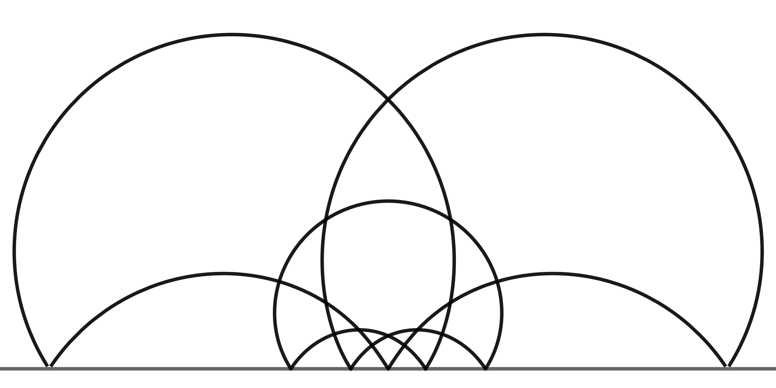
(c) $K=0.4$

(d) $K=2$

Figure 6. Profile curves of CGC surfaces of hyperbolic rotation in the half plane model: for an appropriate choice of parameter, the solutions given in Table 3 yield closed profile curves, see Example 6.7. In the case $K=0.4$ the profile curves are obtained by the second and fourth solutions in the table. The surfaces obtained by hyperbolic rotation of the profile curves in Figures 6(a), 6(c) and 6(d) are shown in Figures 8(d), 8(e), and 8(f), respectively.

6.5. CGC surfaces of parabolic rotation in $\mathbb{H}^{3}$

For surfaces of parabolic rotation in $\mathbb{H}^{3}$, we equip ${\{v\in\mathbb{R}^{4,2}|(v,\mathfrak{q})=-1,\leavevmode\nobreak\ (v,\mathfrak{p})=0\}\cong\mathbb{R}^{3,1}}$ with the pseudo-orthonormal basis $(\mathfrak{v}_{1},\mathfrak{v}_{2},\mathfrak{e}_{1},\mathfrak{e}_{2})$ as in the beginning of Subsection 5.2.1. In that subsection, we gave formulas for the coordinate functions of parabolic rotational surfaces of constant Gauss curvature in hyperbolic spaces of arbitrary (negative) curvature. For $\kappa=-1$, the solutions given in (46) are real if

• $K-1\geq 0$ with $C\geq 0$,

• $K<0$ with $C\leq 0$, or

• $K\in(0,1)$ without restrictions on $C$.

In the last case, the solutions given in (46) are real functions, though a Jacobi transformation has to be applied for this fact to manifest itself. The respective (real) solutions are listed in Table 4 and complement the following classification theorem:

Theorem 6.8.

Every constant Gauss curvature $K\neq 0$ surface of parabolic rotation in $\mathbb{H}^{3}\subset\mathbb{R}^{3,1}$ is given, in terms of a pseudo-orthonormal basis, by

$$(s,\theta)\mapsto\left(\tfrac{r^{2}(s)\left(\theta^{2}+\psi^{2}(s)\right)+1}{2r(s)},r(s),\leavevmode\nobreak\ r(s)\theta,\leavevmode\nobreak\ r(s)\psi(s)\right),$$

where $r$, $\psi$ are as listed in Table 4.

Remark 6.9.

In the third case, $K\in(0,1)$, the solution $\psi$ of (47) comes with an imaginary argument, hence a Jacobi transformation needs to be applied, see Appendix A. The effect is that $\psi$ then contains an elliptic integral of the second kind with modulus $p$, denoted by $E_{p}$ and defined as

$$E_{p}(s)=\int_{0}^{s}\sqrt{1-p^{2}\sin^{2}(u)}du.$$

(a) $K=-1$

(b) $K=0.4$, first $\operatorname{nc}$-solution

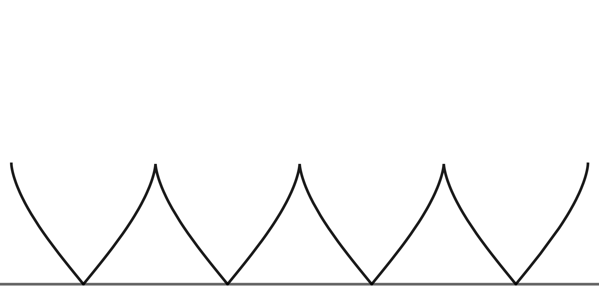
(c) $K=0.4$, second $\operatorname{nc}$-solution

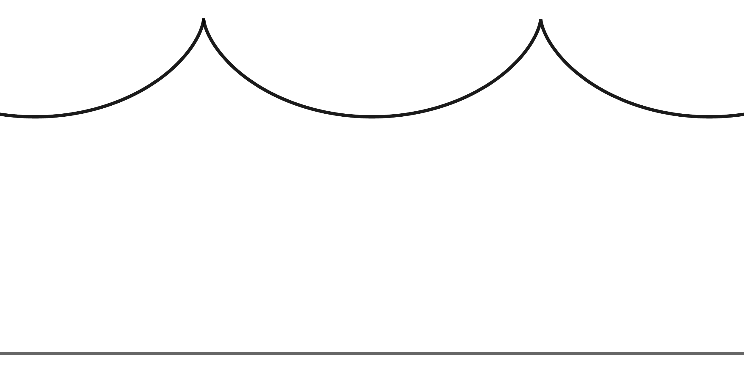
(d) $K=2$

Figure 7. Profile curves of CGC surfaces of parabolic rotation in the half plane model: the profile curves are obtained using the solutions in Table 4. In the Poincaré half space model, the parabolic rotation appears as a translation along the direction perpendicular to the half plane. In Figures 8(g), 8(h), and 8(i), the surfaces obtained from the profile curves in Figures 7(a), 7(b), and 7(d), respectively, are shown in the Poincaré ball model.

$K<0$	$r(s)=\sqrt{\frac{C}{K}}\leavevmode\nobreak\ \operatorname{dn}_{p}\left(\Xi\leavevmode\nobreak\ s\right)$	$\psi(s)=K\leavevmode\nobreak\ s-\tfrac{K}{\Xi}\leavevmode\nobreak\ \Pi\!\left(p^{2};\left.\Xi\leavevmode\nobreak\ s\right|p\right)$
	$\Xi=\sqrt{(K-1)C}$, with $C\leq 0$,	$p=\sqrt{\tfrac{1}{1-K}}$
$K\in(0,1)$	$r(s)=\sqrt{\tfrac{C}{K-1}}\operatorname{nc}_{p}(\Xi\leavevmode\nobreak\ s)$	$\psi(s)=\tfrac{1}{\Xi}\leavevmode\nobreak\ \left(E_{p}\circ\operatorname{am}_{p}\right)(\Xi\leavevmode\nobreak\ s)$
	$\Xi=\sqrt{-C}$ with $C<0$,	$p=\sqrt{1-K}$
	$r(s)=\sqrt{\tfrac{C}{K}}\operatorname{nc}_{p}(\Xi\leavevmode\nobreak\ s)$	$\psi(s)=s-\tfrac{1}{\Xi}\leavevmode\nobreak\ \left(E_{p}\circ\operatorname{am}_{p}\right)(\Xi\leavevmode\nobreak\ s)$,
	$\Xi=\sqrt{C}$, with $C>0$,	$p=\sqrt{K}$
$K=1$	$r(s)=p\leavevmode\nobreak\ \cosh\leavevmode\nobreak\ \left(ps\right)$	$\psi(s)=s+\tfrac{\tanh(ps)}{p}$
	$p\in(0,\infty)$
$K-1>0$	$r(s)=\sqrt{\frac{C}{K-1}}\operatorname{dn}_{p}\left(\Xi\leavevmode\nobreak\ s\right)$	$\psi(s)=K\leavevmode\nobreak\ s-\tfrac{K-1}{\Xi}\leavevmode\nobreak\ \Pi\!\left(p^{2};\left.\Xi\leavevmode\nobreak\ s\right|p\right)$
	$\Xi=\sqrt{KC}$, with $C\geq 0$,	$p=\sqrt{\tfrac{1}{K}}$

Table 4. Parameter functions of CGC surfaces of parabolic rotation in $\mathbb{H}^{3}$.

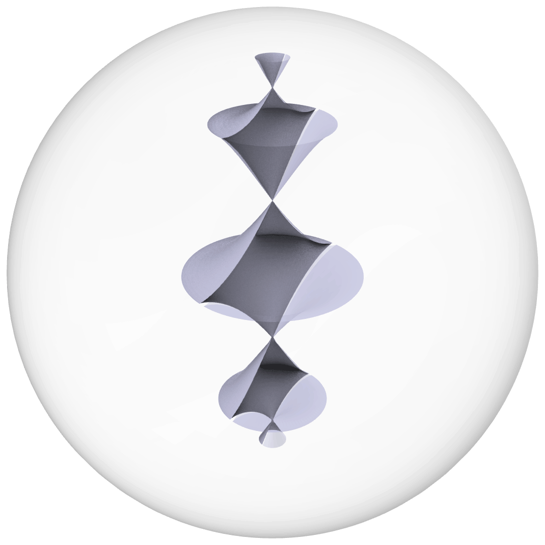
(a) Elliptic rotation, ${K=-1}$, corresponds to the profile curve given in Figure 4(a).

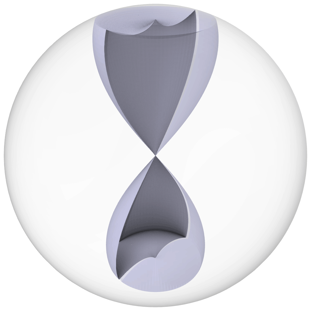
(b) Elliptic rotation, ${K=0.4}$, corresponds to the profile curve given in Figure 4(c).

(c) Elliptic rotation, ${K=2}$, corresponds to the profile curve given in Figure 4(g).

(d) Hyperbolic rotation, ${K=-1}$, corresponds to the profile curve given in Figure 6(a).

(e) Hyperbolic rotation, ${K=0.4}$, corresponds to the profile curve given in Figure 6(c).

(f) Hyperbolic rotation, ${K=2}$, corresponds to the profile curve given in Figure 6(d).

(g) Parabolic rotation, ${K=-1}$, corresponds to the profile curve given in Figure 7(a).

(h) Parabolic rotation, ${K=0.4}$, corresponds to the profile curve given in Figure 7(b).

(i) Parabolic rotation, ${K=2}$, corresponds to the profile curve given in Figure 7(d).

Figure 8. Surfaces of different Gauss curvatures and types of rotation in the Poincaré ball model.

The Theorems 6.3, 6.5 and 6.8 provide explicit parametrisations of all rotational CGC surfaces in $\mathbb{H}^{3}$. Moreover, via parallel transformations, we may obtain parametrisations of all rotational linear Weingarten surfaces in the parallel families of a rotational CGC surface. Thus, Theorem 4.7 and Proposition 2.8 lead to the following theorem.

Theorem 6.10.

Every channel linear Weingarten surface in hyperbolic space $\mathbb{H}^{3}$, satisfying

$$aK+2bH+c=0\leavevmode\nobreak\ \text{with}\leavevmode\nobreak\ \left|\tfrac{a+c}{2}\right|>|b|$$

is parallel to a rotational surface parametrised by one of the parametrisations given in Theorems 6.3, 6.5, or 6.8.

Appendix A Jacobi elliptic functions

We gather some results and transformation formulas for Jacobi elliptic functions and elliptic integrals. For details see [30, Chap 63] and [1, Chap 16 and 17].

A.1. Elliptic functions

The Jacobi elliptic functions of pole type $n$ may be given for a modulus $p\in[0,1]$ by their characterising elliptic differential equations

$$y^{\prime 2}(s)=(1-y^{2}(s))(1-p^{2}y^{2}(s))\leavevmode\nobreak\ \Rightarrow\leavevmode\nobreak\ y(s)=\operatorname{sn}_{p}(s),$$

$$y^{\prime 2}(s)=(1-y^{2}(s))(q^{2}+p^{2}y^{2}(s))\leavevmode\nobreak\ \Rightarrow\leavevmode\nobreak\ y(s)=\operatorname{cn}_{p}(s),$$

$$y^{\prime 2}(s)=(1-y^{2}(s))(-q^{2}+y^{2}(s))\leavevmode\nobreak\ \Rightarrow\leavevmode\nobreak\ y(s)=\operatorname{dn}_{p}(s),$$

where $q=\sqrt{1-p^{2}}$ is called the complementary modulus. The Jacobi amplitude function $\operatorname{am}_{p}$ may be defined via $\operatorname{am}_{p}(s)=\operatorname{arcsin}\operatorname{sn}_{p}(s)=\operatorname{arccos}\operatorname{cn}_{p}(s)$, then the characterising differential equations imply $\operatorname{am}_{p}^{\prime}=\operatorname{dn}_{p}$. Further, we obtain the Pythagorean laws

$$\operatorname{sn}_{p}^{2}+\operatorname{cn}_{p}^{2}=\operatorname{dn}_{p}^{2}+p^{2}\operatorname{sn}_{p}^{2}=1.$$

A wider class of Jacobi elliptic functions may be defined via algebraic combinations of the three functions of pole type $n$:

$$\operatorname{ef}_{p}(s):=\tfrac{\operatorname{en}_{p}(s)}{\operatorname{fn}_{p}(s)}\leavevmode\nobreak\ \textrm{and}\leavevmode\nobreak\ \operatorname{ne}_{p}(s)=\tfrac{1}{\operatorname{en}_{p}(s)},\leavevmode\nobreak\ \textrm{for}\leavevmode\nobreak\ e,f\in\{c,d,s\}.$$

The Jacobi elliptic functions take complex arguments: purely imaginary arguments are evaluated using Jacobi’s imaginary transformations

$$\operatorname{sn}_{p}(is)=i\operatorname{sc}_{q}(s),\quad\operatorname{cn}_{p}(is)=\operatorname{nc}_{q}(s),\quad\operatorname{dn}_{p}(is)=\operatorname{dc}_{q}(s).$$

Note that $\operatorname{cn}$ and $\operatorname{dn}$ are real functions of imaginary arguments, whereas $\operatorname{sn}$ becomes imaginary.

The restriction $p\in[0,1]$ on the modulus $p$ can be lifted by means of Jacobi’s real transformations:

$$\operatorname{sn}_{\tfrac{1}{p}}(s)=p\operatorname{sn}_{p}\left(\tfrac{s}{p}\right),\quad\operatorname{cn}_{\tfrac{1}{p}}(s)=\operatorname{dn}_{p}\left(\tfrac{s}{p}\right),\quad\operatorname{dn}_{\tfrac{1}{p}}(s)=\operatorname{cn}_{p}\left(\tfrac{s}{p}\right),$$

allow evaluation for $p\geq 1$, and by definition, all Jacobi elliptic functions are even with respect to their modulus. Also, with respect to an imaginary modulus $ip\in i\mathbb{R}$, the Jacobi elliptic functions take real values for a real argument: the corresponding transformations read

$$\begin{array}[]{l}\operatorname{sn}_{ip}(s)=q^{\prime}\operatorname{sd}_{p^{\prime}}\left(s\sqrt{1+p^{2}}\right),\vspace{5pt}\\ \operatorname{cn}_{ip}(s)=\operatorname{cd}_{p^{\prime}}\left(s\sqrt{1+p^{2}}\right)\vspace{5pt},\\ \operatorname{dn}_{ip}(s)=\operatorname{nd}_{p^{\prime}}\left(s\sqrt{1+p^{2}}\right).\end{array}\leavevmode\nobreak\ \textrm{with}\leavevmode\nobreak\ p^{\prime}=\tfrac{p}{\sqrt{1+p^{2}}},$$

A.2. Elliptic integrals

The elliptic integrals are closely related to Jacobi’s elliptic functions. According to [1, Chap 17] the (incomplete) elliptic integral of first, second and third kind, denoted by $F$, $E$ and $\Pi$, respectively, is

$$F(s,p) =\int_{0}^{s}\tfrac{du}{\sqrt{1-p^{2}\sin^{2}(u)}},$$

$$E(s,p) =\int_{0}^{s}\sqrt{1-p^{2}\sin^{2}(u)}\leavevmode\nobreak\ du,$$

$$\Pi(k;s,p) =\int_{0}^{s}\tfrac{1}{1-k\sin^{2}(u)}\tfrac{du}{\sqrt{1-p^{2}\sin^{2}(u)}},$$

where $p\in[0,1]$ as before. Evaluated at $s=\pi/2$, we obtain $F_{p}$ ($E_{p}$, $\Pi^{k}_{p}$) the complete elliptic integrals of first (second, third) kind. $F_{p}$ is of particular interest: The functions $\operatorname{sn}_{p}$ and $\operatorname{cn}_{p}$ are periodic with period $4F_{p}$, whilst $\operatorname{dn}_{p}$ is periodic with period $2F_{p}$. For this note, it is useful to introduce notation for the composition of elliptic integrals with the amplitude function $\operatorname{am}$. We will denote

$$F(\operatorname{am}_{p}(s),p) =:F(s|p),$$

$$E(\operatorname{am}_{p}(s),p) =:E(s|p),$$

$$\Pi(k;\operatorname{am}_{p}(s),p) =:\Pi\!\left(k;\left.s\right|p\right).$$

In Section 5, we utilise transformation formulas for $\Pi$, which can be written as

$$\Pi\!\left(k;\left.s\right|p\right)=\int_{0}^{s}\tfrac{du}{1-k\operatorname{sn}_{p}^{2}(u)}.$$

In this form, we see that $\Pi$ is a real function for all $p\in\mathbb{R}$ and for imaginary arguments, since $\operatorname{sn}$ has real or imaginary values in these cases. Using Jacobi’s transformations of the last subsection, we learn

$$\Pi\!\left(k;\left.as\right|\tfrac{1}{p}\right)=p\leavevmode\nobreak\ \Pi\!\left(kp^{2};\left.\tfrac{as}{p}\right|p\right),$$

$$\Pi\!\left(k;\left.i\leavevmode\nobreak\ as\right|p\right)=\left\{\begin{array}[]{l}p^{2}\tfrac{i\leavevmode\nobreak\ as}{q^{2}}-\tfrac{i}{q^{2}}E(s|q),\leavevmode\nobreak\ \textrm{for}\leavevmode\nobreak\ k=1,\\ \tfrac{i\leavevmode\nobreak\ as}{1-k}-\tfrac{ik}{1-k}\leavevmode\nobreak\ \Pi\!\left(1-k;\left.as\right|q\right),\leavevmode\nobreak\ \textrm{for}\leavevmode\nobreak\ k\neq 1,\end{array}\right.$$

$$\Pi\!\left(k;\left.as\right|ip\right)=\tfrac{ap^{\prime 2}}{k^{\prime}}\leavevmode\nobreak\ s+\tfrac{kq^{\prime 3}}{k^{\prime}}\Pi\!\left(k^{\prime};\left.\tfrac{as}{q^{\prime}}\right|p^{\prime}\right),$$

for $a\in\mathbb{R}^{\times}$ with $p^{\prime},q^{\prime}$ as in the last section and $k^{\prime}=p^{\prime 2}+kq^{\prime 2}$.

References

- [1] M. Abramowitz and I. Stegun, editors. Handbook of Mathematical Functions: With Formulas, Graphs, and Mathematical Tables. Dover Books on Mathematics. Dover Publ, New York, NY, 9. dover print edition, 1972.
- [2] J. Arroyo, O. J. Garay, and A. Pámpano. Delaunay surfaces in . Filomat, 33(4):1191–1200, 2019.
- [3] A. Barros, J. Silva, and P. Sousa. Rotational linear Weingarten surfaces into the Euclidean sphere. Isr. J. Math., 192(2):819–830, 2012.
- [4] W. Blaschke. Vorlesungen über Differentialgeometrie und geometrische Grundlagen von Einsteins Relativitätstheorie III. Springer Berlin Heidelberg, 1929.
- [5] F. E. Burstall, U. Hertrich-Jeromin, M. Pember, and W. Rossman. Polynomial Conserved Quantities of Lie Applicable Surfaces. manuscripta math., 158(3-4):505–546, 2019.
- [6] F. E. Burstall, U. Hertrich-Jeromin, and W. Rossman. Lie geometry of flat fronts in hyperbolic space. C. R. Acad. Sci., Paris, 348(11):661–664, 2010.
- [7] F. E. Burstall, U. Hertrich-Jeromin, and W. Rossman. Lie geometry of linear Weingarten surfaces. C. R. Acad. Sci., Paris, 350(7):413–416, 2012.
- [8] F. E. Burstall, U. Hertrich-Jeromin, and W. Rossman. Discrete linear Weingarten surfaces. Nagoya Math. J., 231:55–88, 2018.
- [9] F. E. Burstall and S. Santos. Special isothermic surfaces of type . Journ. London Math. Soc., 85(2):571–591, 2012.
- [10] T. E. Cecil. Lie Sphere Geometry: With Applications to Submanifolds. Universitext. Springer, New York, 2nd ed edition, 2008.
- [11] G. Darboux. Lecons sur la théorie générale des surfaces, volume II. Gauthier-Villars, 1889.
- [12] C. Delaunay. Sur la surface de révolution dont la courbure moyenne est constante. J. Math. Pures et Appl., pages 309–314, 1841.
- [13] A. Demoulin. Sur les surfaces . C. R. Acad. Sci., Paris, 153:927–929, 1911.
- [14] A. Demoulin. Sur les surfaces et les surfaces . C. R. Acad. Sci., Paris, 153:590–593, 705–707, 1911.
- [15] A. Doliwa. Geometric discretization of Koenigs nets. J. Math. Phys., 44:2234 – 2249, 2003.
- [16] U. Dursun. Rotational Weingarten surfaces in hyperbolic 3-space. J. Geom., 111(1):7, 2020.
- [17] D. Ferus and F. Pedit. Isometric immersions of space forms and soliton theory. Math. Ann., 305(1):329–342, 1996.
- [18] J. M. Gomes. Spherical surfaces with constant mean curvature in hyperbolic space. Bol. Soc. Bras. Mat, 18(2):49–73, 1987.
- [19] U. Hertrich-Jeromin. Introduction to Möbius Differential Geometry. Cambridge University Press, Cambridge, 2003.
- [20] U. Hertrich-Jeromin, K. Mundilova, and E.-H. Tjaden. Channel linear Weingarten surfaces. J. Geom. Symmetry Phys., 40(7):25–33, 2015.
- [21] U. Hertrich-Jeromin, W. Rossman, and G. Szewieczek. Discrete channel surfaces. Math. Z., 294(1):747–767, 2020.
- [22] M. Kokubu, W. Rossman, M. Umehara, and K. Yamada. Flat fronts in hyperbolic 3-space and their caustics. J. Math. Soc. Japan, 59, 2005.
- [23] M. Kokubu, M. Umehara, and K. Yamada. Flat fronts in hyperbolic 3-space. Pac. J. Math., 216, 2003.
- [24] R. López. Linear Weingarten surfaces in Euclidean and hyperbolic space. arXiv:0906.3302 [math], 2009.
- [25] R. Lopez. Parabolic surfaces in hyperbolic space with constant Gaussian curvature. Bull. Belg. Math. Soc., 16, 2009.
- [26] R. S. Palais and C. Terng. Critical Point Theory and Submanifold Geometry. Number 1353 in Lecture Notes in Mathematics. Springer, Berlin, 1988.
- [27] A. Pámpano. A variational characterization of profile curves of invariant linear Weingarten surfaces. Differ. Geom. Appl., 68:101564, 2020.
- [28] M. Pember and G. Szewieczek. Channel surfaces in Lie sphere geometry. Beitr. Algebra Geom., 59(4):779–796, 2018.
- [29] D. Polly. Linear Weingarten channel surfaces. Master’s thesis, TU Wien, Wien, 2017.
- [30] J. Spanier and K. B. Oldham. An Atlas of Functions. Hemisphere Pub. Corp, Washington, 1987.
- [31] E. Vessiot. Contribution à la géometrie conforme. Théorie des surfaces. Bull. S. M. F., 54:139–179, 1926.