ResVGAE: Going Deeper with Residual Modules for Link Prediction

Abstract

Graph autoencoders are efficient at embedding graph-based data sets. Most graph autoencoder architectures have shallow depths which limits their ability to capture meaningful relations between nodes separated by multi-hops. In this paper, we propose Residual Variational Graph Autoencoder, ResVGAE, a deep variational graph autoencoder model with multiple residual modules. We show that our multiple residual modules, a convolutional layer with residual connection, improve the average precision of the graph autoencoders. Experimental results suggest that our proposed model with residual modules outperforms the models without residual modules and achieves similar results when compared with other state-of-the-art methods.

1 Introduction

Learning-based feature extraction approaches have led to better performance in machine learning tasks, such as computer vision, machine translation, and object detection. Most real-world data sets have proven to be very successful in producing data representations that are successfully used in several tasks, such as fraud detection Wang et al. [2019], recommendation systems Feng et al. [2019], churn prediction Liu et al. [2018] and predicting earthquakes using graph processes Ruiz et al. [2019]. Graph neural networks (GNN) can efficiently exploit the relationship between data set instances in non-Euclidean space. Different variants of graph autoencoders, Shi et al. [2020], Yu et al. [2021],  Weng et al. [2020], Davidson et al. [2018], Perozzi et al. [2014a], have been very successful in capturing meaningful representations for node classification Grover and Leskovec [2016], link prediction Vilnis and McCallum [2015] and graph classification Tu et al. [2018] tasks.

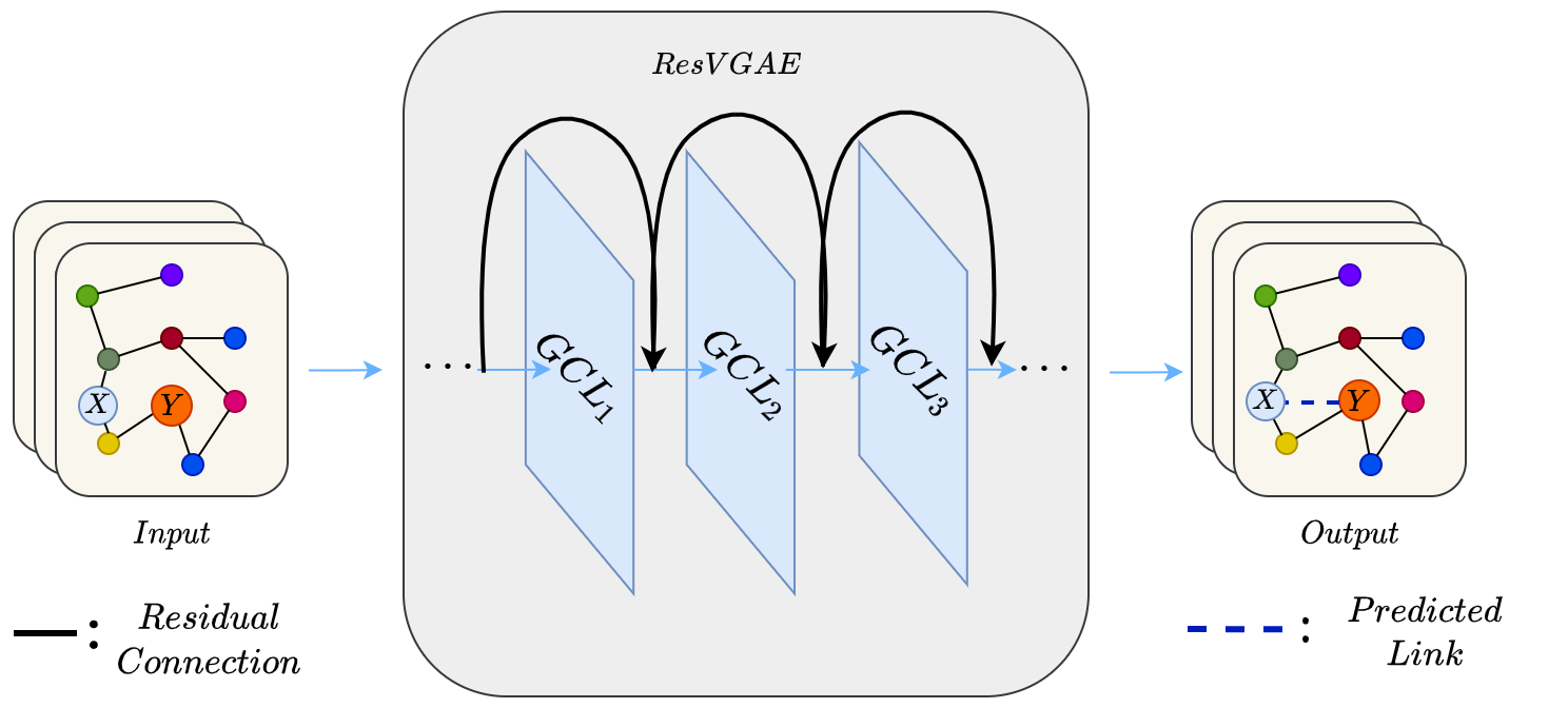
Figure 1: End-to-end framework of ResVGAE. Given two distant nodes $X$ and $Y$, the model predicts a link (blue dashed line in the output) between them. This is made possible efficiently, thanks to the residual modules (residual connections with their consecutive Graph Convolutional Layers (GCLs). Here, we show a model with three modules, namely, $GCL_{1}$, $GCL_{2}$, and $GCL_{3}$.

In recent years, we see a proliferation of graph embedding techniques for improving graph convolutional networks and their applications in graph-structured data sets Scardapane et al. [2018]. Perozzi et al. propose DeepWalk, a framework that embeds graph nodes based on the information acquired from truncated random walks. The framework is robust and can learn meaningful node representations for large-scale data sets Perozzi et al. [2014b], whereas Grover et al. presents a framework that maps node features in a low-dimensional space while preserving the networks neighborhoods of nodes Grover and Leskovec [2016]. Tang et al. propose another classical approach that is capable of network embedding while preserving first and second-order proximities of the nodes Tang et al. [2015]. Another method that embeds graph data sets is Deep Variational Network Embedding in Wasserstein Space (DVNE), a network embedding framework that uses a 2-Wasserstein distance as a similarity measure between the latent node distributions. The proposed framework preserves the first-order and second-order node proximities in the network Zhu et al. [2018]. GraphSAGE is a framework that generates inductive node embeddings for previously unseen data by leveraging node features. In this work, the authors train a set of aggregator functions that learn from the neighbor’s node features Hamilton et al. [2017], whereas Pan et al. propose an adversarially regularized variational graph autoencoder (ARVGA), a framework where the latent representations are enforced to match prior distributions using an adversarial training scheme Pan et al. [2018]. Several theoretical works have pointed out the occurrence of the over-smoothing phenomenon, the process in which node representations become indistinguishable when nodes interact with other nodes they are not directly connected, Chen et al. [2020], Alon and Yahav [2021], Mavromatis and Karypis [2021], Zhou et al. [2020]. This limits the ability of the models to stack many GNN layers. We want deep graph networks to capture long-distance interactions between far nodes for link prediction tasks. As shown in Fig.1, to capture meaningful information between distant nodes $X$ and node $Y$, our model embeds the nodes into a similar low-dimensional vector space. If the node embeddings are similar, then our model predicts a link between them. In this example, nodes $X$ and $Y$ are three hops apart so ResVGAE has three residual modules.

We propose a model architecture with residual modules that combines residual connections He et al. [2016] and variational graph autoencoders (cf. Fig.2) in order to alleviate the over-smoothing phenomenon.

The overall contributions of our study are as follows:

• We propose a graph variational autoencoder model with residual modules and compare it with the other state-of-the-art models for link prediction tasks.

• We measure the accuracy of adding residual modules on similar graph-based autoencoders with different depths.

• We study the over-smoothing phenomena by implementing our proposed architecture from one up to eight residual modules.

The rest of the paper is organized as follows: Section 2 covers the proposed model architectures. In Section 3, comparative results of the proposed ResVGAE model are presented for the link prediction task on three benchmark data sets. We conclude the paper and propose new research paths for future work in Section 4.

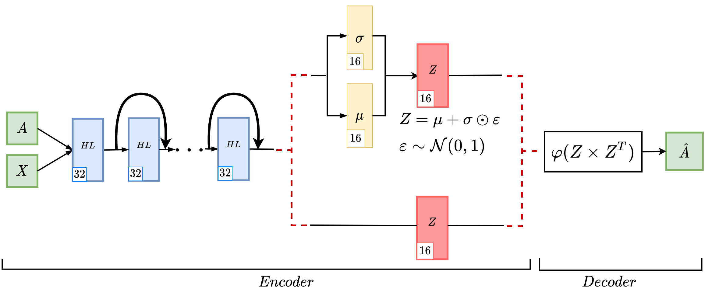
Figure 2: Model architecture of ResVGAE. Residual connections start after the first Hidden Layer ($HL$) since the input and the output size of layers with residual modules must be the same. The encoder takes the adjacency matrix $A$ and the feature matrix $X$ as inputs and outputs the node embeddings $Z$. The decoder takes as input the embedding matrix $Z$ and outputs the reconstructed adjacency matrix $\hat{A}$. The blocks in blue indicate the graph convolutional layers that embed 32-dimensional node feature vectors into a matrix. Similarly, yellow blocks constitute the graph convolutional layers that embed 16-dimensional hidden layer features into the output Z matrix. The upper and lower branches of the encoder represent variational graph autoencoder and graph autoencoder architectures, respectively.

2 Method

Graph autoencoders are deep learning frameworks whose inputs are instance features and adjacency matrices and whose output is the reconstructed adjacency matrix. These frameworks mainly consist of two components, namely, the encoder and the decoder. The encoder part transforms the input into a lower-dimensional embedding while the decoder part transforms the embedding into the reconstructed adjacency matrix. Let $G=(V,E)$ denote a graph $G$, where $V$ is the set with $N$ nodes, and $E$ is the set of edges. Moreover, let $v_{i}\in V$ denote a node and $e_{ij}=(v_{i},v_{j})$ denote an edge between two nodes $v_{i}$ and $v_{j}$. We define the adjacency matrix $A$ as:

$$A:=\left\{\begin{array}[]{ll}A_{ij}=1,&\text{e}_{ij}\in E\\ A_{ij}=0,&\text{e}_{ij}\notin E\\ \end{array}\right.$$ (1)

where $A$ is a symmetric matrix. Let $X$ be the feature matrix of the nodes. For all the encoder architectures, we use the graph convolutional layer proposed by Kipf and Welling [2017]. The layer follows the propagation rule:

$$H^{(l+1)}=\varphi\left(\tilde{D}^{-\frac{1}{2}}\tilde{A}\tilde{D}^{-\frac{1}{2}}H^{(l)}W^{(l)}\right)$$ (2)

where $\varphi$ is the sigmoid activation function, $\tilde{D}$ is the degree matrix, $\tilde{A}$ is the normalized adjacency matrix with self-loops and $W^{(l)}$ is the layer’s weight matrix. In a multi-layer model $H^{(0)}=X$ and $H^{(l)}$ is the feature map of the $l^{th}$ layer.

Variational graph encoders transform the graph into a lower-dimensional embedding, using graph convolutional layers and a sampling layer. These graph convolutional layers transform the graph into the desired lower-dimensional space and produces mean and standard deviation values using two layers. Then, the sampling layer takes these mean and deviation values to generate samples from the prior distribution. Hence the generated samples constitute the embedding of the graph.

The final embeddings are encoded as a distribution over the latent space as:

$$q(Z\mid X,A)=\prod_{i=1}^{N}q\left(z_{i}\mid X,A\right)$$ (3)

where

$$q\left(z_{i}\mid X,A\right)=\mathcal{N}\left(\mu_{i},\operatorname{diag}\left(\sigma^{2}\right)\right)$$ (4)

Here, $z_{i}$ is the embedding vectors for node $i$; $\mu_{i}$ and $\sigma$ are the graph convolutional layer vector outputs of the encoder.

Using this structure provides a graph embedding with the desired distribution (cf. Fig.2).

For the graph autoencoder models, the decoder is a non-probabilistic model that reconstructs the adjacency matrix by computing the inner-product of the latent representations of two-node embeddings :

$$\hat{A}=\varphi\left(ZZ^{T}\right)$$ (5)

In all the models, $\varphi(\cdot)$ denotes the sigmoid activation function.

For the graph variational autoencoder models, the decoder is a probabilistic model that reconstructs the adjacency matrix by computing the probabilistic inner product of the latent representation of nodes:

$$p(A\mid Z)=\prod_{i=1}^{N}\prod_{j=1}^{N}p\left(A_{ij}\mid z_{i},z_{j}\right)$$ (6)

where

$$p\left(A_{ij}\mid z_{i},z_{j}\right)=\varphi\left(z_{i}^{T}z_{j}\right)$$ (7)

Vanilla models are trained by minimizing reconstruction loss:

$$\mathcal{L}=\mathbb{E}_{q(Z\mid X,A)}[\log p(A\mid Z)]$$ (8)

and variational models are optimized by maximizing the variational lower bound while minimizing reconstruction loss:

$$\mathcal{L}=\mathbb{E}_{q(Z\mid X,A)}[\log p(A\mid Z)]-\mathrm{KL}[q(Z\mid X,A)\|p(Z)]$$ (9)

where $\mathrm{KL}[q(\cdot)\|p(\cdot)]$ is the Kullback-Leibler divergence between $q(\cdot)$ and $p(\cdot)$ . The posterior distribution is approximated by a Gaussian distribution using the reparametrization trick Kingma and Welling [2014]. Our proposed method, ResVGAE is a variational graph autoencoder with multiple residual modules. The decoder and loss are the same as variational graph autoencoders. To improve the performance of the variational graph autoencoder, we propose utilizing residual modules in the encoder similar to (2). A residual module can be represented as:

$$H^{(l+1)}=\varphi\left(\tilde{D}^{-\frac{1}{2}}\tilde{A}\tilde{D}^{-\frac{1}{2}}H^{(l)}W^{(l)}\right)+H^{(l)}$$ (10)

The input and the output sizes of the hidden layers must be the same to add residual modules. The number of residual modules can be determined depending on the depth of exploration among nodes for link prediction.

3 Experimental Results

We evaluate the model’s performance on three benchmark data sets: Cora McCallum et al. [2000], CiteSeer Giles et al. [1998] and PubMed Namata et al. [2012]. Cora and CiteSeer are networks of computer science publications where the nodes represent the publications and the edges represent the citations. The PubMed data set is also a citation network that contains a set of articles related to diabetes disease.

We compare ResVGAE against three baseline algorithms: Deep Walk (DW)Perozzi et al. [2014a], Spectral Clustering (SC) Tang and Liu [2011] and Adversarially Regularized Graph Autoencoder (ARVGE) Pan et al. [2018]

All models and data sets in this paper have been used for link prediction tasks and Table 1 gives a detailed summary of the data sets we used.

Table 1: Data set statistics

Data set	# Nodes	# Edges	# Classes	# Features
CitesSeer	3,327	4,732	6	3,703
Cora	2,708	5,429	7	1,433
PubMed	19,717	44,338	3	500

We evaluate all the models based on the same baseline as in Kipf and Welling [2016] and we use AP and AUC scores to report the average precision of 10 runs with random train, validation, and test splits of the same size, and all the models are trained for 200 epochs. The validation and test sets contain 5% and 10% of the total edges, respectively. The embedding dimensions of the node features for the hidden layers is 32 and the embedding dimension of node features for the output layer is 16. The models are optimized using the Adam optimizer with a learning rate of 0.01.

In our experiments, we use average precision (AP) and area under ROC curve (AUC) metrics to measure the accuracy of our models. We use PyTorch Geometric Fey and Lenssen [2019] and our code will be available upon acceptance.

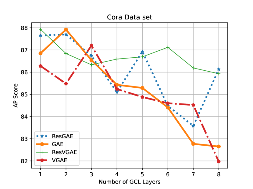
Figure 3: The AP scores of the models with multiple numbers of layers for the Cora data set. ResGAE has the highest AP score followed by ResVGAE and the graph autoencoders without the residual modules. Residual modules substantially improve the performance of the variational autoencoder models in comparison to models without them. The performance gap increases for a higher number of layers.

Experiments indicate that, for shallow models, all proposed models achieve similar average precision scores. Here we see that all models with one residual module embed the node features in a very similar way. The score differs when we use models with deeper networks.

In models with eight graph convolutional layers, we see that models with residual modules have higher average precision scores than models without residual modules. In Fig. 3, we run all the models from one up to eight graph convolutional layers. Here we see that as the models become deeper their average precision decreases significantly. The models with residual modules achieve higher scores than the models without residual modules.

Plots in Figs. 4 and  5 indicate the steady drop in average precision values for all the models on CiteSeer and PubMed data sets, respectively. Moreover, for deeper models, the results suggest that deep models with residual modules outperform the models without residual modules.

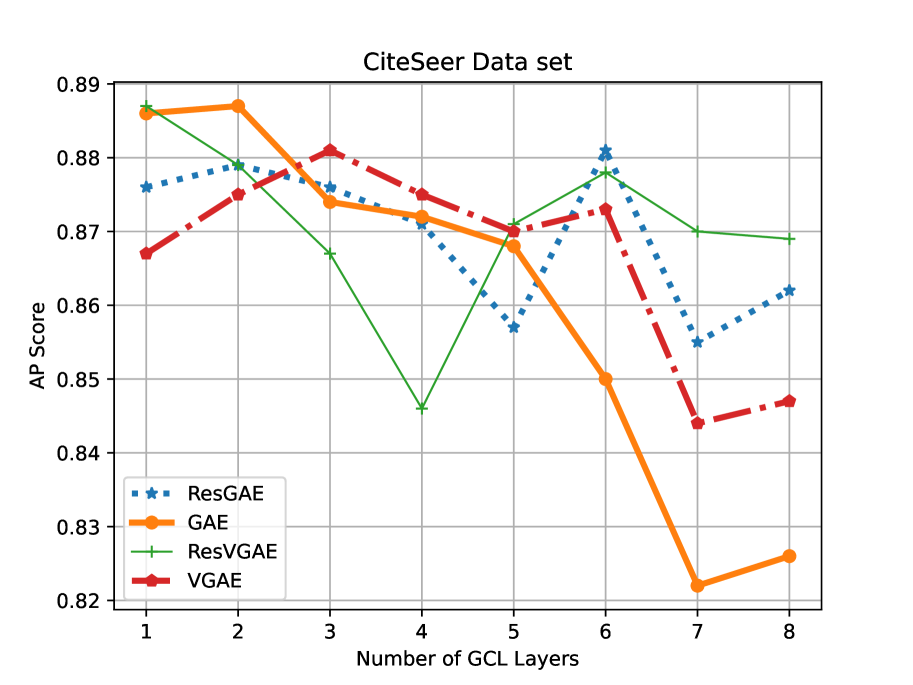
Figure 4: The AP scores of the models with a different number of GCL layers for the CiteSeer data set. Models with residual modules score higher than the models without residual modules. The highest scoring model is ResVGAE followed by ResGAE for the number of layers seven and eight.

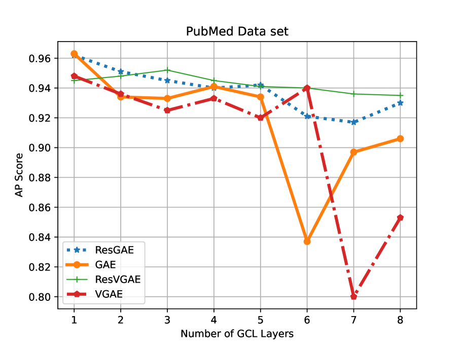
Figure 5: The AP scores of the models with a different number of GCL layers for the PubMed data set. Residual modules with more layers result in a higher AP score.

Table 2: Performance comparison of models with and without residual modules. Our proposed architectures, ResVGAE and ResGAE, achieve higher AUC and AP scores on Cora, CiteSeer, and PubMed data sets when compared to their variational graph autoencoder counterparts without residual modules.

Method	Cora		CiteSeer		PubMed
	AUC	AP	AUC	AP	AUC	AP
ResVGAE (Ours)	$\textbf{85.93}\pm\textbf{1.02}$	$\textbf{88.55}\pm\textbf{0.65}$	$\textbf{86.90}\pm\textbf{1.85}$	$\textbf{80.30}\pm\textbf{0.40}$	$\textbf{91.28}\pm\textbf{0.80}$	$\textbf{93.50 }\pm\textbf{0.68}$
VGAE	$81.97\pm 0.79$	$85.51\pm{2.54}$	$83.70\pm 0.77$	$79.00\pm 0.60$	$85.30\pm 0.95$	$82.60\pm 0.60$
ResGAE (Ours)	$\textbf{86.13}\pm\textbf{0.844}$	$\textbf{88.85}\pm\textbf{0.31}$	$\textbf{87.10}\pm 1\textbf{.99}$	$\textbf{84.40}\pm\textbf{1.95}$	$\textbf{93.00}\pm\textbf{0.46}$	$\textbf{91.40}\pm\textbf{0.29}$
GAE	$82.65\pm 0.79$	$86.46\pm 0.32$	$82.60\pm 1.28$	$81.60\pm 1.17$	$90.60\pm 1.70$	$87.80\pm 0.90$

Improvement in terms of average precision values is evident for models with residual models tested on Cora, CiteSeer, and PubMed data sets (Table 2). More specifically, ResVGAE outputs higher AUC and AP scores than VGAE, and the difference in score is significant when compared with GAE for CiteSeer and PubMed data sets. For the Cora data set, we see that ResGAE performs better than ResVGAE and the other graph autoencoders without residual modules.

Furthermore, in Table 3, we compare our model with other baseline models on link prediction tasks. Our model outperforms Spectral Clustering and DeepWalk algorithms in all three datasets and scores a very similar result to the ARVGE algorithm on the Cora and PubMed datasets.

Tests on publicly available data sets reveal the importance of architectures with residual modules for exploring the interactions among far nodes for link prediction tasks. In models without residual modules, variational graph autoencoder scores higher in the CiteSeer data sets whereas graph autoencoder outperforms graph variational autoencoder in the Cora and PubMed data sets.

Table 3: Performance comparison of models with other baseline models.

Models	Cora		Citeseer		PubMed
	AUC	AP	AUC	AP	AUC	AP
DW	$83.1\pm 0.01$	$85.0\pm 0.00$	$80.5\pm 0.02$	$83.6\pm 0.01$	$84.4\pm 0.00$	$84.1\pm 0.00$
SC	$84.6\pm 0.01$	$88.5\pm 0.00$	$80.5\pm 0.01$	$85.0\pm 0.01$	$84.2\pm 0.02$	$87.8\pm 0.01$
ARVGE	${92.4}\pm{0.004}$	$92.6\pm 0.004$	${92.4}\pm{0.003}$	${93.0}\pm{0.003}$	$96.5\pm 0.001$	$96.8\pm 0.001$
ResVGAE	${87.93}\pm{1.90}$	$90.23\pm 1.35$	${88.7}\pm{1.53}$	${84.47}\pm{0.53}$	$94.5\pm 0.64$	$94.8\pm 0.20$

4 Conclusion

In this paper, we introduce ResVGAE, a variational graph autoencoder with residual modules to mitigate the over-smoothing phenomenon occurring in graph neural networks with deep architectures. Results indicate that the proposed model scores similar average precisions for shallow models and outperforms variational graph autoencoders without residual modules for link prediction task among nodes with multi-hop separation.

As a future research direction, we plan to test our models’ performance on larger benchmark data sets and focus on other tasks such as graph classification, node classification, and graph clustering. Furthermore, we intend to experiment with the effect of the inclusion of residual modules with different distributions for the variational graph autoencoders.

Acknowledgments

This work is supported by The Scientific and Technological Research Council of Turkey (TÜBİTAK) under Project No. 121E378 and by Istanbul Technical University (ITU) Vodafone Future Lab under Project No. ITUVF20180901P04.

Declarations

• Funding: Noted in the acknowledgments section

• Conflict of interest/Competing interests Not applicable

• Ethics approval: Not applicable

• Consent to participate: Not applicable

• Consent for publication: All authors’ consent

• Availability of data and materials: Upon request

• Code availability: Available upon acceptance and can be shared with editors at any time

• Authors’ contributions: All authors consent

References

- Wang et al. [2019] Jianyu Wang, Rui Wen, Chunming Wu, Yu Huang, and Jian Xion. Fdgars: Fraudster detection via graph convolutional networks in online app review system. In Companion Proceedings of The 2019 World Wide Web Conference, pages 310–316, 2019.
- Feng et al. [2019] Chenyuan Feng, Zuozhu Liu, Shaowei Lin, and Tony QS Quek. Attention-based graph convolutional network for recommendation system. In ICASSP 2019-2019 IEEE International Conference on Acoustics, Speech and Signal Processing (ICASSP), pages 7560–7564. IEEE, 2019.
- Liu et al. [2018] Xi Liu, Muhe Xie, Xidao Wen, Rui Chen, Yong Ge, Nick Duffield, and Na Wang. A semi-supervised and inductive embedding model for churn prediction of large-scale mobile games. In 2018 IEEE International Conference on Data Mining (ICDM), pages 277–286. IEEE, 2018.
- Ruiz et al. [2019] Luana Ruiz, Fernando Gama, and Alejandro Ribeiro. Gated graph convolutional recurrent neural networks. In 2019 27th European Signal Processing Conference (EUSIPCO), pages 1–5. IEEE, 2019.
- Shi et al. [2020] Han Shi, Haozheng Fan, and James T Kwok. Effective decoding in graph auto-encoder using triadic closure. In Proceedings of the AAAI Conference on Artificial Intelligence, volume 34, pages 906–913, 2020.
- Yu et al. [2021] Bin Yu, Yu Zhang, Yu Xie, Chen Zhang, and Ke Pan. Influence-aware graph neural networks. Applied Soft Computing, 104:107169, 2021.
- Weng et al. [2020] Ziqiang Weng, Weiyu Zhang, and Wei Dou. Adversarial attention-based variational graph autoencoder. IEEE Access, 8:152637–152645, 2020.
- Davidson et al. [2018] Tim R. Davidson, Luca Falorsi, Nicola De Cao, Thomas Kipf, and Jakub M. Tomczak. Hyperspherical variational auto-encoders. 34th Conference on Uncertainty in Artificial Intelligence (UAI-18), 2018.
- Perozzi et al. [2014a] Bryan Perozzi, Rami Al-Rfou, and Steven Skiena. Deepwalk: Online learning of social representations. In Proceedings of the 20th ACM SIGKDD international conference on Knowledge discovery and data mining, pages 701–710. ACM, 2014a.
- Grover and Leskovec [2016] Aditya Grover and Jure Leskovec. node2vec: Scalable feature learning for networks. In Proceedings of the 22nd ACM SIGKDD international conference on Knowledge discovery and data mining, pages 855–864, 2016.
- Vilnis and McCallum [2015] Luke Vilnis and Andrew McCallum. Word representations via gaussian embedding. CoRR, abs/1412.6623, 2015.
- Tu et al. [2018] Ke Tu, Peng Cui, Xiao Wang, Fei Wang, and Wenwu Zhu. Structural deep embedding for hyper-networks. In AAAI, pages 426–433, 2018. URL https://www.aaai.org/ocs/index.php/AAAI/AAAI18/paper/view/16797.
- Scardapane et al. [2018] Simone Scardapane, Steven Van Vaerenbergh, Danilo Comminiello, and Aurelio Uncini. Improving graph convolutional networks with non-parametric activation functions. In 2018 26th European Signal Processing Conference (EUSIPCO), pages 872–876, 2018. 10.23919/EUSIPCO.2018.8553465.
- Perozzi et al. [2014b] Bryan Perozzi, Rami Al-Rfou, and Steven Skiena. Deepwalk: Online learning of social representations. In Proceedings of the 20th ACM SIGKDD international conference on Knowledge discovery and data mining, pages 701–710, 2014b.
- Tang et al. [2015] Jian Tang, Meng Qu, Mingzhe Wang, Ming Zhang, Jun Yan, and Qiaozhu Mei. Line: Large-scale information network embedding. In Proceedings of the 24th International Conference on World Wide Web, WWW ’15, page 1067–1077, Republic and Canton of Geneva, CHE, 2015. International World Wide Web Conferences Steering Committee. ISBN 9781450334693. 10.1145/2736277.2741093. URL https://doi.org/10.1145/2736277.2741093.
- Zhu et al. [2018] Dingyuan Zhu, Peng Cui, Daixin Wang, and Wenwu Zhu. Deep variational network embedding in wasserstein space. In Proceedings of the 24th ACM SIGKDD International Conference on Knowledge Discovery & Data Mining, pages 2827–2836. ACM, 2018.
- Hamilton et al. [2017] Will Hamilton, Zhitao Ying, and Jure Leskovec. Inductive representation learning on large graphs. Advances in neural information processing systems, 30, 2017.
- Pan et al. [2018] Shirui Pan, Ruiqi Hu, Guodong Long, Jing Jiang, Lina Yao, and Chengqi Zhang. Adversarially regularized graph autoencoder for graph embedding. arXiv preprint arXiv:1802.04407, 2018.
- Chen et al. [2020] Deli Chen, Yankai Lin, Wei Li, Peng Li, Jie Zhou, and Xu Sun. Measuring and relieving the over-smoothing problem for graph neural networks from the topological view. In Proceedings of the AAAI Conference on Artificial Intelligence, volume 34, pages 3438–3445, 2020.
- Alon and Yahav [2021] Uri Alon and Eran Yahav. On the bottleneck of graph neural networks and its practical implications. In International Conference on Learning Representations, 2021. URL https://openreview.net/forum?id=i80OPhOCVH2.
- Mavromatis and Karypis [2021] Costas Mavromatis and George Karypis. Graph infoclust: Maximizing coarse-grain mutual information in graphs. In Pacific-Asia Conference on Knowledge Discovery and Data Mining, pages 541–553. Springer, 2021.
- Zhou et al. [2020] Jie Zhou, Ganqu Cui, Shengding Hu, Zhengyan Zhang, Cheng Yang, Zhiyuan Liu, Lifeng Wang, Changcheng Li, and Maosong Sun. Graph neural networks: A review of methods and applications. AI Open, 1:57–81, 2020.
- He et al. [2016] Kaiming He, Xiangyu Zhang, Shaoqing Ren, and Jian Sun. Deep residual learning for image recognition. In Proceedings of the IEEE conference on computer vision and pattern recognition, pages 770–778, 2016.
- Kipf and Welling [2017] Thomas N. Kipf and Max Welling. Semi-supervised classification with graph convolutional networks. In 5th International Conference on Learning Representations, ICLR 2017, Toulon, France, April 24-26, 2017, Conference Track Proceedings, 2017. URL https://openreview.net/forum?id=SJU4ayYgl.
- Kingma and Welling [2014] Diederik P. Kingma and Max Welling. Auto-Encoding Variational Bayes. In 2nd International Conference on Learning Representations, ICLR 2014, Banff, AB, Canada, April 14-16, 2014, Conference Track Proceedings, 2014.
- McCallum et al. [2000] Andrew Kachites McCallum, Kamal Nigam, Jason Rennie, and Kristie Seymore. Automating the construction of internet portals with machine learning. Information Retrieval, 3(2):127–163, 2000.
- Giles et al. [1998] C Lee Giles, Kurt D Bollacker, and Steve Lawrence. Citeseer: An automatic citation indexing system. In ACM DL, pages 89–98, 1998.
- Namata et al. [2012] Galileo Namata, Ben London, Lise Getoor, Bert Huang, and UMD EDU. Query-driven active surveying for collective classification. In 10th International Workshop on Mining and Learning with Graphs, volume 8, 2012.
- Tang and Liu [2011] Lei Tang and Huan Liu. Leveraging social media networks for classification. Data Mining and Knowledge Discovery, 23(3):447–478, 2011.
- Kipf and Welling [2016] Thomas Kipf and Max Welling. Variational graph auto-encoders. ArXiv, abs/1611.07308, 2016.
- Fey and Lenssen [2019] Matthias Fey and Jan E. Lenssen. Fast graph representation learning with PyTorch Geometric. In ICLR Workshop on Representation Learning on Graphs and Manifolds, 2019.