Poroelastic near-field inverse scattering
Abstract
A multiphysics data analytic platform is established for imaging poroelastic interfaces of finite permeability (e.g., hydraulic fractures) from elastic waveforms and/or acoustic pore pressure measurements. This is accomplished through recent advances in design of non-iterative sampling methods to inverse scattering. The direct problem is formulated via the Biot equations in the frequency domain where a network of discontinuities is illuminated by a set of total body forces and fluid volumetric sources, while monitoring the induced (acoustic and elastic) scattered waves in an arbitrary near-field configuration. A thin-layer approximation is deployed to capture the rough and multiphase nature of interfaces whose spatially varying hydro-mechanical properties are a priori unknown. In this setting, the well-posedness analysis of the forward problem yields the admissibility conditions for the contact parameters. In light of which, the poroelastic scattering operator and its first and second factorizations are introduced and their mathematical properties are carefully examined. It is shown that the non-selfadjoint nature of the Biot system leads to an intrinsically asymmetric factorization of the scattering operator which may be symmetrized at certain limits. These results furnish a robust framework for systematic design of regularized and convex cost functionals whose minimizers underpin the multiphysics imaging indicators. The proposed solution is synthetically implemented with application to spatiotemporal reconstruction of hydraulic fracture networks via deep-well measurements.
keywords:
poroelastic waves, waveform tomography, hydraulic fractures, multiphysics sensing1 Introduction
Coupled physics processes driven by engineered stimulation of the subsurface underlie many emerging technologies germane to advanced energy infrastructure such as unconventional hydrocarbon and geothermal reservoirs [1, 2]. Optimal design and closed-loop control of such systems require real-time feedback on the nature of progressive variations in a target region [3, 4]. 3D in-situ tracking of multiphasic developments however is exceptionally challenging [5, 6]. Engineered treatments (such as fluid or gas injection) often occur in a complex background whose structure and hydro-mechanical properties are uncertain [7, 8]. Nevertheless, state-of-the-art solutions to in-situ characterization mostly rely on elastic waves [9, 10, 11, 4]. In particular, micro-seismic waves generated during shear propagation of fractures are commonly used to monitor evolving discontinuities in rock [12, 13]. Such passive schemes are nonetheless agnostic to aseismic evolution [14], and involve significant assumptions on the nature of wave motion in the subsurface which may lead to critical errors [15, 16, 17]. On the other hand, existing approaches to full waveform inversion [18, 19, 11], while offering more comprehensive solutions, are by and large computationally expensive and thus inapplicable for real-time sensing. Therefore, there exists a critical need for the next generation of imaging technologies that transcend some of these limitations.
In this vein, recent advances in rigorous design of sampling-based waveform tomography solutions [20, 21, 22, 23, 24] seem particularly relevant owing to their robustness and newfound capabilities pertinent to imaging in complex and unknown domains [21, 23, 25, 26]. So far, these developments mostly reside in the context of self-adjoint and energy preserving systems such as Helmholtz and Navier equations. Wave attenuation, however, is a defining feature of the fractured rock systems with crucial impact on subsurface exploration [27, 28, 29]. In this context, a systematic analysis of sound absorption – e.g., due to the fluid-solid interaction, and its implications on sampling-based data inversion is still lacking. This, in part, may be due to the sparse and single-physics nature of traditional data. Fast-paced progress in sensing instruments such as fiber optic (FBG) sensors – capturing high-resolution multiple physical measurements in time-space [12, 30], may bridge this gap and enable a holistic approach to subsurface characterization. This invites new data analytic tools capable of (a) expedited processing of large datasets, and (b) simultaneous inversion of multiphysics observations. The latter may particularly assist a high-fidelity reconstruction of the sought-for subterranean events.
In this paper, the theoretical foundation of poroelastic inverse scattering is established with application to spatiotemporal tracking of hydraulic fracture networks in unconventional energy systems. This method is nested within the framework of active sensing where the process zone is sequentially illuminated (during stimulation) via deep-well excitations prompting poroelastic scattering whose signature is recorded in the form of seismic and pore pressure waveforms. Thus-obtained multiphase sensory data are deployed for geometric reconstruction of treatment-induced evolution in the target region. Rooted in rigorous foundations of the inverse scattering theory [24], the proposed imaging solution carries a high spatial resolution with carefully controlled sensitivity to noise and illumination frequency.
The forward problem is posed in a suitable dimensional platform catering for simultaneous elastic and acoustic data inversion. A system of arbitrary-shaped hydraulic fractures with non-trivial (i.e., heterogeneous, dissipative, and finitely permeable) interfaces is illuminated by a plausible combination of total body forces and fluid volumetric sources in a medium governed by the coupled Biot equations [31, 32]. Thus-induced multiphase scattered fields are used to define the poroelastic scattering operator mapping the source densities to near-field measurements. In this setting, the reconstruction scheme is based on (i) a custom factorization of the near-field operator, and (b) a sequence of approximate solutions to the scattering equation, seeking (fluid and total-force) source densities whose affiliated waveform pattern matches that of a designated poroelastodynamics solution emanating from a sampling point. The latter is obtained via a sequence of carefully constructed cost functionals whose minimizers can be computed without iterations. Such minimizing solutions are then used to construct a robust multiphysics imaging indicator whose performance is examined through a set of numerical experiments.
In what follows, Section 2 introduces the direct scattering problem and the necessary tools for the inverse analysis. In particular, Section 2.4 investigates the well-posedness of the forward problem which leads to finding the admissibility conditions for the interfacial contact parameters including the elastic stiffness matrix and the permeability, effective stress and Skempton coefficients. This criteria plays a key role later in Section 3 where the essential properties of the poroelastic scattering operator and its components, in the first and second factorizations, are established. Section 4 presents the regularized cost functionals for solving the scattering equations, main theorems, and imaging functionals. Section 5 illustrates a set of numerical experiments implementing the reconstruction of (stationary and evolving) hydraulic fracture networks via the near-field measurements by way of the proposed imaging indicators.
2 Problem statement
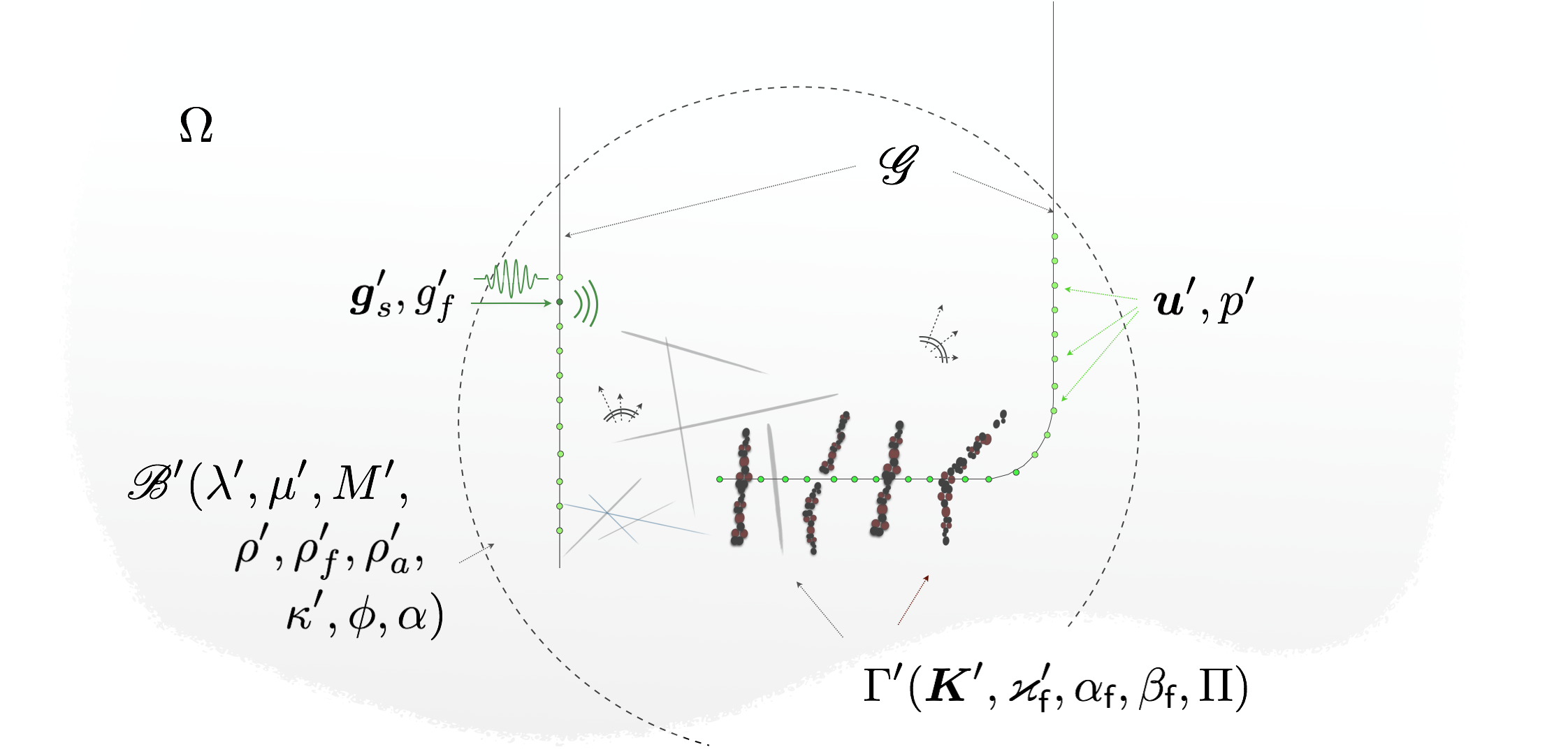
Consider the ball of radius , centered at the origin in the subsurface , encompassing the stimulation zone and sensing grid as illustrated in Fig. 1. Let be sufficiently large so that the probing waves may be assumed negligible in due to poroelastic attenuation. It is also assumed that does not meet , which in hydraulic fracturing is a reasonable premise, in particular, since a treatment region is typically four to ten kilometers below the surface while m [33]. The domain is described by drained Lamé coefficients and , Biot modulus , total density , fluid density , apparent mass density , permeability coefficient , porosity , and Biot effective stress coefficient . A system of pre-existing and stimulation-induced fractures and flow networks is embedded in whose rough and multiphasic interfaces are characterized by a set of heterogeneous parameters, namely: the stiffness matrix , permeability coefficient , effective stress coefficient , Skempton coefficient , and fluid pressure dissipation factor on . The domain is excited by time harmonic total body forces of density and fluid volumetric sources of density on at frequency . This gives rise to poroelastic scattering observed on the sensing grid in terms of solid displacements and pore pressure .
2.1 Dimensional platform
To enable multiphasic data inversion, the reference scales
| (1) |
are respectively defined for stress, mass density, and length. Here, denotes the solid-phase density. Note that represents the drained shear wavelength. In this setting, all physical quantities are rendered dimensionless [34] as follows
| (2) | ||||
2.2 Field equations
The incident field generated by in the background is governed by
| (3) | |||||
where is the fourth-order drained elasticity tensor with denoting the th-order symmetric identity tensor, and
| (4) |
The interaction of with gives rise to the scattered field solving
| in | (5) | |||||
| in | ||||||
| on | ||||||
| on | ||||||
| on |
where and are defined by
| (6) | |||||
the unit normal on is explicitly identified in Section 2.3;
signifies the jump in across , while
is the respective mean fields on ; , according to [35], is a symmetric and possibly complex-valued matrix of specific stiffnesses which in the fracture’s local coordinates may be described as the following
| (7) |
wherein and are known respectively as the tangential and normal drained elastic stiffnesses. It should be mentioned that the contact condition across makes use of the generalized Schoenberg’s model for a poroelatic interface of finite permeability [35].
Remark 2.1.
The contact law at high-permeability interfaces [35] is reduced to the following form
| on | |||||
| on | |||||
| on |
where on .
The formulation of the direct scattering problems may now be completed by requiring that and satisfy the radiation condition as [36]. On uniquely decomposing the incident and scattered fields into two irrotational parts (, ) and a solenoidal part (s) as
| (8) |
the radiation condition can be stated as
| (9) | ||||
uniformly with respect to where , , is the complex-valued wavenumber associated with the slow and fast p-waves and the transverse s-wave [37].
2.3 Function spaces
For clarity of discussion, it should be mentioned that the support of may be decomposed into smooth open subsets , , such that . The support of may be arbitrarily extended to a closed Lipschitz surface of a bounded simply connected domain . In this setting, the unit normal vector to coincides with the outward normal vector to . Let be a multiply connected Lipschitz domain of bounded support such that , then is assumed to be an open set relative to with a positive surface measure, and the closure of is denoted by . Following [38], we define
| (10) | ||||
and recall that and are respectively the dual spaces of and . Accordingly, the following embeddings hold
| (11) |
Note that since , then by trace theorems , , and .
2.4 Poroelastic scattering
In this section, the poroelastic scattering operator is introduced and its first and second factorizations are formulated. In what follows, the Einstein’s summation convention applies over the repeated indexes.
2.4.1 Incident wave function
Observe that for a given density , the poroelastic incident field solving (3) may be recast in the integral form
| (14) |
whose kernel is the poroelastodynamics fundamental solution tensor provided in A. Here, signifies the component of the solid displacement at due to a unit total body force applied at along the coordinate direction , while is the associated pore pressure. Likewise, stands for the solid displacement at in the direction due to a unit fluid source i.e., volumetric injection at , and is the induced pore pressure.
2.4.2 Poroelastic scattered field
By way of the reciprocal theorem of poroelastodynamics [39, 40], one may show that the following integral representation holds for the scattered field satisfying (5)-(9),
| (15) |
whose kernel is derived from the fundamental solution tensor and provided in A. More specifically, and indicate the fundamental tractions on ; and signify the associated relative fluid-solid displacements across ; and are the fundamental pore pressure solutions.
2.4.3 Poroelastic scattering operator
The linearity of (5) implies that the scattered wave function may be expressed as a linear integral operator. To observe this, let be a constant vector characterizing an incident point source wherein indicates the amplitude and direction of the total body force, while represents the magnitude of fluid volumetric source both applied at . The resulting scattered field is observed in terms of seismic displacements and pore pressure at . Now, let us define the scattering kernel so that
| (16) |
Then, given , one may easily verify that
| (17) |
Accordingly, one may define the poroelastic scattering operator by
| (18) |
2.4.4 Factorization of
With reference to (3) and (6), let us define the operator given by
| (19) |
where specifies the incident field traction, is the specific relative fluid-solid displacement across , and is the incident pore pressure on . Next, define as the map taking the incident traction, relative flow and pressure over to the multiphase scattered data satisfying (5)-(9). Then, the scattering operator (18) may be factorized as
| (20) |
Lemma 2.1.
The adjoint operator takes the form
| (21) |
where solves
| in | (22) | |||||
| in | ||||||
| on |
Here, the ‘bar’ indicates complex conjugate, and
Note that satisfy the radiation condition as , similar to the complex conjugate of (9).
Proof.
see C. ∎
3 Key properties of the poroelastodynamic operators
Lemma 3.1.
Operator in Lemma 2.1 is compact, injective, and has a dense range.
Proof.
See D. ∎
Lemma 3.2.
Operator in (23) is bounded and satisfies
| (25) |
Proof.
See E. ∎
Lemma 3.3.
Operator : (i) has a bounded (and thus continuous) inverse, and (ii) is coercive, i.e., there exists constant independent of such that
| (26) |
Proof.
See F. ∎
Lemma 3.4.
Operator is compact over .
Proof.
Lemma 3.5.
The poroelastic scattering operator is injective, compact and has a dense range.
Proof.
See G. ∎
4 Inverse poroelastic scattering
This section presents an adaptation of the key results from sampling approaches to inverse scattering for the problem of poroelastic-wave imaging of finitely permeable interfaces. The fundamental idea stems from the nature of solution to the poroelastic scattering equation
| (27) |
where is the near-field pattern of a trial poroelastodynamic field specified by Definition 1.
Definition 1.
With reference to (15), for every admissible density specified over a smooth, non-intersecting trial interface , the induced near-field pattern is given by
| (28) |
Remark 4.1.
In light of (27), one may interpret the philosophy of sampling-based waveform tomography as the following. Let (containing the origin) denote a poroelastic discontinuity whose characteristic size is small relative to the length scales describing the forward scattering problem, and let where and is a unitary rotation matrix. Given a density , solving the scattering equation (27) over a grid of trial pairs sampling is simply an effort to probe the range of operator (or that of ), through synthetic reshaping of the illuminating wavefront, for fingerprints in terms of . As shown by Theorems 4.2, such fingerprint is found in the data if and only if . Otherwise, the norm of any approximate solution to (27) can be made arbitrarily large, which provides a criterion for reconstructing .
Theorem 4.1.
Under the assumptions of Remark 2.2 for the wellposedness of the forward scattering problem, for every smooth and non-intersecting trial dislocation and density profile , one has
Proof.
The argument directly follows that of [41, Theorem 6.1]. ∎
On the basis of Theorem 4.1, one arrives at the following statement which inspires the sampling-based poroelastic imaging indicators.
Theorem 4.2.
Under the assumptions of Theorem 4.1,
-
1.
If , there exists a density vector such that and
. -
2.
If , then such that , one has
.
Proof.
The argument directly follows that of [41, Theorem 6.2]. ∎
4.1 The multiphysics indicator
Theorem 4.2 poses two challenges in that: (i) the featured indicator inherently depends on the unknown support of hidden scatterers, and (ii) construction of the wavefront density is implicit in the theorem [20, 26]. These are conventionally addressed by replacing with which in turn is computed by way of Tikhonov regularization [42] as follows.
First, note that when the measurements are contaminated by noise (e.g., sensing errors and fluctuations in the medium properties), one has to deal with the noisy operator satisfying
| (29) |
where is a measure of perturbation in data independent of . Assuming that is compact, the Tikhonov-regularized solution to (27) is obtained by non-iteratively minimizing the cost functional defined by
| (30) |
where the regularization parameter is obtained by way of the Morozov discrepancy principle [42]. On the basis of (30), the well-known linear sampling indicator is constructed as
| (31) |
By design, achieves its highest values at the loci of hidden scatterers . More specifically, the behavior of within may be characterized as the following,
| (32) | ||||
4.2 The modified indicator
In cases where the illumination frequency and/or the background’s permeability is sufficiently large so that according to (4), one may deduce from (22)-(24) that the second factorization of the poroelastic scattering operator is symmetrized as follows,
| (33) |
In this setting, one may deploy the more rigorous indicator [41] to dispense with the approximations underlying the imaging functional. This results in a more robust reconstruction especially with noisy data [26]. The indicator takes advantage of the positive and self-adjoint operator defined on the basis of the scattering operator by
| (34) |
with the affiliated factorization [43]
| (35) |
where in light of Lemma 3.3, the middle operator is coercive with reference to [41, Lemma 5.7] i.e., there exists a constant independent of such that ,
| (36) |
Thanks to (36), the term in Theorem 4.2 may be safely replaced by which is computable without prior knowledge of .
In presence of noise, the perturbed operator is deployed satisfying
| (37) |
which is assumed to be compact similar to in (29). Then, the regularized cost functional is constructed according to [23, Theorems 4.3],
| (38) |
Here, represents the regularization parameter specified in terms of from (30) as
| (39) |
In addition, signifies both a measure of perturbation in data and a regularization parameter that, along with , is designed to create a robust imaging indicator as per Theorems 4.3. It should be mentioned that is convex and that its minimizer solves the linear system
| (40) |
which can be computed without iterations [23]. Within this framework, the following theorem rigorously establishes the relation between the range of operator and the norm of penalty term in (38).
Theorem 4.3.
In this setting, the imaging indicator takes the form
| (42) |
with similar characteristics to as in (32) yet more robustness against noise [26].
Remark 4.2.
It is worth noting that the sampling-based characterization of from near-field data is deeply rooted in geometrical considerations, so that the fracture indicator functionals (31) and (42) may exhibit only a minor dependence on the complex contact condition – described according to (5) by the heterogeneous distribution of: the stiffness matrix , permeability coefficient , effective stress coefficient , Skempton coefficient , and fluid pressure dissipation factor on . This attribute may be traced back to Remark 4.1 where the opening displacement profile – which is intimately related to the interface law, is deemed arbitrary (within the constraints of admissibility). This quality makes the proposed imaging paradigm particularly attractive in situations where the interfacial parameters are unknown a priori, which opens possibilities for the sequential geometrical reconstruction and interfacial characterization of such anomalies e.g., see [44, 45].
Remark 4.3.
It should be mentioned that there are recent efforts to systematically adapt the indicator for application to asymmetric scattering operators [21]. These developments, however, do not lend themselves to poroelastic inverse scattering due to the non-selfadjoint nature of . A fundamental treatment of the poroelastic indicator in the general case where could be an interesting subject for a future study.
5 Computational treatment and results
This section examines the performance of multiphasic indicators (31) and (42) through a set of numerical experiments. In what follows, the synthetic data are generated within the FreeFem++ computational platform [46].
5.1 Testing configuration
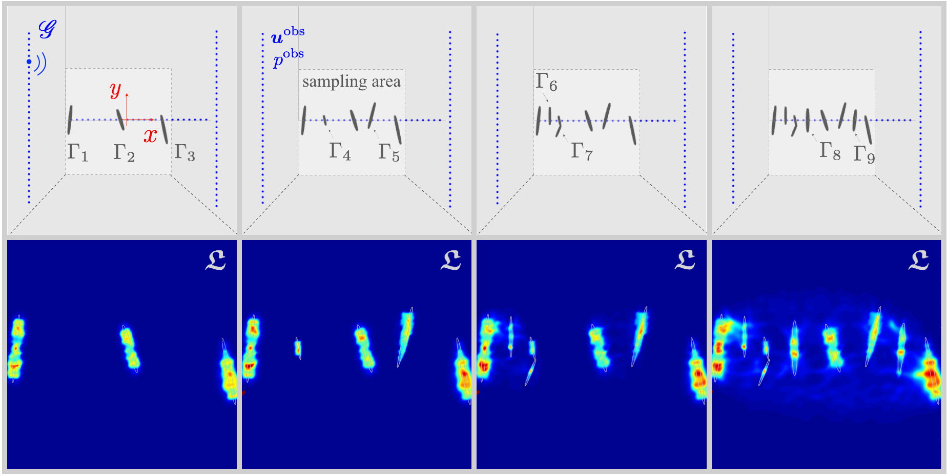
Two test setups shown in Figs. 2 and 3 are considered where the background is a poroelastic slab of dimensions endowed with (evolving and stationary) hydraulic fracture networks. Following [47, 48], the properties of Pecos sandstone are used to characterize . On setting the reference scales GPA, kg/m3, and m for stress, mass density, and length, respectively, the non-dimensionalized quantities of Table 1 are obtained and used for simulations. Accordingly, the complex-valued wave speeds [16] affiliated with the modal decomposition in (8) read , , and . The boundary condition on is such that the total traction and pore pressure vanish for both incident and scattered fields i.e., . In Setup I, a hydraulic fracture network is induced in four steps as shown in Fig. 2. A detailed description of scatterers including the center , length , and orientation of each crack , is provided in Table 2. All fractures in this configuration are highly permeable as per Remark 2.1 and characterized by the interfacial stiffness , effective stress coefficient , and Skempton coefficient on . The latter quantities are taken from [35]. Note that in Setup I, the excitation and sensing grid straddles two (vertical) monitoring wells and the horizontal section of the injection well. Depicted in Figs. 3 and 4, Setup II features hydraulic fractures of distinct length scales as described in Table 3. The discontinuity interfaces in this configuration are modeled as thin poroelastic inclusions characterized by , , , , and , while the remaining material parameters are similar to their counterparts in the background as reported in Table 1. In Setup II, the excitation and measurements are solely conducted in the treatment well shown in Fig. 3.
| property | value | dimensionless value |
|---|---|---|
| first Lamé parameter (drained) | 2.74 GPA | 0.47 |
| drained shear modulus | 5.85 GPA | 1 |
| Biot modulus | 9.71 GPA | 1.66 |
| total density | 2270 kg/m3 | 2.27 |
| fluid density | 1000 kg/m3 | = 1 |
| apparent mass density | 117 kg/m3 | 0.117 |
| permeability coefficient | 0.8 mm/N | 24.5 10 |
| porosity | 0.195 | 0.195 |
| Biot effective stress coefficient | 0.83 | 0.83 |
| frequency | 12 kHz | 3.91 |
| | 1 | 2 | 3 | 4 | 5 | 6 | 7 | 8 | 9 |
|---|---|---|---|---|---|---|---|---|---|
| | | | | | | | | | |
| | | | | | | | | | |
| | | | | | | | | | |
| | | | | | | | | | |
5.2 Forward scattering simulations
Every sensing step entails in-plane harmonic excitation via total body forces and fluid volumetric sources at a set of points on . The excitation frequency is set such that the induced shear wavelength in the specimen is approximately one, serving as a reference length scale. The incident waves interact with the hydraulic fracture network in each setup giving rise to the scattered field , governed by (5), whose pattern over the observation grid is then computed. For both illumination and sensing purposes, is sampled by a uniform grid of excitation and observation points. In Setup I, the H-shaped incident/observation grid is comprised of source/receiver points, while in Setup II, the L-shaped support of injection well is uniformly sampled at points for excitation and sensing.
5.3 Data Inversion
With the preceding data, one may generate the multiphasic indicator maps affiliated with (31) and (42) in three steps, namely by: (1) constructing the discrete scattering operators and from synthetic data , (2) computing the trial signature patterns pertinent to a poroelastic host domain, and (3) evaluating the imaging indicators ( or ) in the sampling area through careful minimization of the discretized cost functionals (30) and (38) as elucidated in the sequel.
Step 1: construction of the multiphase scattering operator
Given the in-plane nature of wave motion, i.e., that the polarization amplitude of excitation and the nontrivial components of associated scattered fields lay in the plane of orthonormal bases , the discretized scattering operator may be represented by a matrix with components
| (43) |
where is the component of the solid displacement measured at due to a unit force applied at along the coordinate direction and is the associated pore pressure measurement; also, u signifies the solid displacement at due to a unit injection at and p is the affiliated pore pressure. Note that here the general case is presented where excitations and measurements are conducted along all dimensions. may be downscaled as appropriate according to the testing setup.
Noisy operator. To account for the presence of noise in measurements, we consider the perturbed operator
| (44) |
where is the identity matrix, and is the noise matrix of commensurate dimension whose components are uniformly-distributed (complex) random variables in . In what follows, the measure of noise in data with reference to definition (29) is .
Step 2: generation of a multiphysics library of scattering patterns
This step aims to construct a suitable right hand side for the discretized scattering equation in unbounded and bounded domains pertinent to the analytical developments of Section 4 and numerical experiments of this section, respectively.
Unbounded domain in . In this case, the poroelastic trial pattern is given by Definition 1 indicating that (a) the right hand side is not only a function of the dislocation geometry but also a function of the trial density , and (b) computing generally requires an integration process at every sampling point . Conventionally, one may dispense with the integration process by considering a sufficiently localized (trial) density function e.g., see [41, 23].
Bounded domain. This case corresponds to the numerical experiments of this section where the background is a poroelastic plate of finite dimensions. In this setting, following [49], it is straightforward to show that the trial patterns for a finite domain is governed by
| in | (45) | |||||
| in | ||||||
| on | ||||||
| on |
In what follows, the trial signatures over the observation grid are computed separately for every sampling point by solving
| in | (46) | |||||
| in | ||||||
| on | ||||||
| on | ||||||
| on |
where , and the trial dislocation is described by an infinitesimal crack wherein is a unitary rotation matrix, and L represents a vanishing penny-shaped crack of unit normal , so that . On recalling (43), the three non-trivial components of in the plane, with orthonormal bases , are arranged into a vector for as the following
| (47) |
Sampling. With reference to Figs. 2 and 3, the search area i.e., the sampling region is a square probed by a uniform grid of sampling points where the featured indicator functionals are evaluated, while the unit circle spanning possible orientations for the trial dislocation is sampled by a grid of trial normal directions , and the excitation form – as a fluid source or an elastic force, is selected via . Accordingly, the multiphasic indicator maps and are constructed through minimizing the cost functionals (30) and (38) for a total of trial triplets .
Remark 5.1.
It is worth mentioning that in the discretized equation
| (48) |
the scattering operators is independent of any particular choice of or .Therefore, one may replace in (48) with an assembled matrix, encompassing all variations of and , to solve only one equation for the reconstruction of hidden fractures which is computationally more efficient.
Step 3: computation of the multiphysics imaging functionals
map. With reference to Theorem 4.2, (48) is solved by minimizing the regularized cost functional (30). It is well-known, however, that the Tikhonov functional is convex and its minimizer can be obtained without iteration [42]. Thus-obtained solution to (48) is a vector (or matrix for all right-hand sides) identifying the structure of multiphasic wavefront densities on . On the basis of (31) and (32), the multiphysics indicator is then computed as
| (49) |
map. In the case where , one may construct a more robust approximate solution to (48) by minimizing in (38). As indicated in Section 4, is also convex and its minimizer can be computed by solving the discretized linear system (40). Then, with reference to (42), the multiphase indicator is obtained as
| (50) |
5.4 Simulation results
Near-field tomography of an evolving network. With reference to Fig. 2, a hydraulic fracture network is induced in in four steps. Following each treatment, the numerical experiments are conducted as described earlier where the multiphasic scattering patterns are obtained over an H-shaped sensing grid resulting in a scattering matrix. The latter is then used to compute the distribution of indicator in the sampling region, at every sensing step, to recover the sequential evolution of the network as shown in the figure.
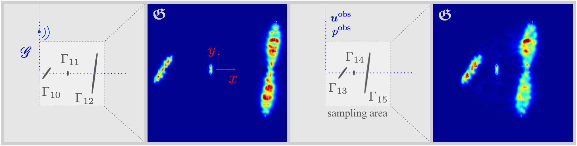
Limited-aperture imaging. Fig. 3 shows the reconstructed maps via (50) from the complete dataset, including both solid displacements and pore pressure measurements , on an L-shaped grid associated with the injection (or treatment) well, which results in a poroelastic scattering matrix. Here, both networks and involve hydraulic fractures of different length scales e.g., is of while is of . One may also observe the interaction between scatterers in the maps when the pair-wise distances between fractures is less than a few wavelengths. It should be mentioned that similar maps are obtained by deploying the imaging functional. However, it is interesting to note that the indicator is successful in reconstructing the fracture network even though . This may be due to the particular sensor arrangement germane to the hydraulic fracturing application where a subset of the sensing grid (within the injection well) is in fact in close proximity of scatterers , .
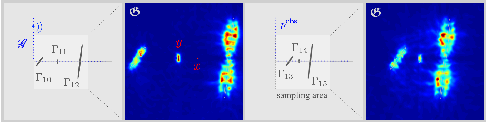
Acoustic imaging via the pore fluid. In hydrofracking, it may be convenient to generate distributed fluid volumetric excitation within the treatment well and simultaneously measure thus-induced pore pressures on the same grid. Data inversion on the basis of acoustic excitation and measurements may expedite reconstruction of the induced fractures. In this spirit, Fig. 4 illustrates the reconstruction results for the network and sensing configurations similar to Fig. 3 where the excitation takes only the form of a fluid volumetric source, and the measurements are pore pressure data . The indicator generates very similar maps.
6 Conclusions
A multiphysics data inversion framework is developed for near-field tomography of hydraulic fracture networks in poroelastic backgrounds. This imaging solution is capable of spatiotemporal reconstruction of discontinuous interfaces of arbitrary (and possibly fragmented) support whose poro-mechanical properties are unknown. The data is processed within an appropriate dimensional framework to allows for simultaneous inversion of elastic and acoustic (i.e., pore pressure) measurements, which are distinct in physics and scale. The proposed imaging indicator is (a) inherently non-iterative enabling fast inversion of dense data in support of real-time sensing, (b) flexible with respect to the sensing configuration and illumination frequency, and (c) robust against noise in data. Limited-aperture and partial data inversion – e.g., deep-well tomography as well as imaging based solely on pore pressure excitation and measurements – are explored. Both and indicators showed success in the numerical experiments germane to the limiting case of high-frequency illumination. It should be mentioned that this imaging modality can be naturally extended to more complex e.g., highly heterogeneous backgrounds. Given the multiphysics nature of data, a remarkable potential would be to deploy this approach within a hybrid data analytic platform to enable not only geometric reconstruction, but also interfacial characterization of discontinuity surfaces, e.g., involving the retrieval of permeability profile of hydraulic fractures from poroelastic data.
7 Acknowledgements
The corresponding author kindly acknowledges the support provided by the National Science Foundation (Grant #1944812). We would like to mention Rezgar Shakeri’s assistance with the preliminary studies on forward scattering by interfaces of infinite permeability. This work utilized resources from the University of Colorado Boulder Research Computing Group, which is supported by the National Science Foundation (awards ACI-1532235 and ACI-1532236), the University of Colorado Boulder, and Colorado State University.
Appendix A Poroelastodynamics fundamental solution
The poroelastodynamics fundamental solution [40, 50] takes the form
| (51) |
where satisfies
| (52) | ||||
while solves
| (53) | ||||
both subject to the relevant radiation conditions similar to (9). On setting
permits the explicit form
| (54) | ||||
and reads
| (55) |
In this setting, the associated fundamental tractions and on a surface characterized by the unit normal vector may be specified as
| (56) | ||||
where Einstein’s summation convention applies over the repeated indexes. In addition, the normal relative fluid-solid displacements and across may be expressed as
| (57) | ||||
Appendix B Wellposedness of the poroelastic scattering problem
Given and the interface operator satisfying (13), then the direct scattering problem (5)-(9) has a unique solution that continuously depends on . Note that is continuously dependent on according to (6). First, observe that (5)-(9) may be expressed on in the variational form in terms of so that satisfying the radiation condition (9),
| (58) | ||||
where is defined by
with the ‘bar’ indicating complex conjugate. Note that in light of (9), one has
It is worth mentioning that (58) is obtained by premultiplying the first of (5) by and its second by ; the results are then added and integrated by parts over . The duality pairing on the left hand side of (58) is continuous with respect to , , and owing to the continuity of the trace mapping from into . Now let us define subject to (9), the coercive operator
| (59) | ||||
On invoking i.e., from Section 2.1 and recalling from (4) that , one may observe
| (60) | ||||
for a constant independent of . Next, define subject to (9), the compact operator
| (61) | ||||
where
for a constant c independent of and . Then, the compact embedding of into and the compactness of the trace operator indicates that B defines a compact perturbation of . Therefore, on letting , one may observe that the problem (58) is of Fredholm type, and thus, is well-posed as soon as the uniqueness of a solution is guaranteed. Assume that . Then, on invoking (4) and (12), one may show that when ,
| (62) |
where
| (63) |
It should be mentioned that (62) is obtained by (a) premultiplying the first of (5) by , (b) conjugating the second of (5) and multiplying the results by , and (c) integrating by parts over and adding the results. On letting , one finds (62) indicating that in by the premise of Remark 2.2. As a result, the first equation in (5) will be reduced to the Navier equation that is subject to the (exponentially decaying) poroelastodynamics radiation conditions (9) which implies that in . The second equation in (5) then reads in which completes the proof for the uniqueness of a scattering solution, and thus, substantiates the wellposedness of the forward problem.
Appendix C Proof of Lemma 2.1
Appendix D Proof of Lemma 3.1
Observe that of Lemma 2.1 possesses the integral form
| (66) |
Note that the kernel is derived from the poroelastodynamics fundamental solution of A which also appeared in the integral representation (15). In this setting, the smoothness of substantiates the compactness of as an application from into . Next, suppose that there exists such that . Then, the vanishing trace of on implies, by the unique continuation principle, that in , and whereby which guarantees the injectivity of . The densness of the range of is established via the injectivity of . To observe the latter, let such that . The definition (19) then reads on with satisfying (3). Now, assume that contains (possibly disjoint) analytic surfaces , , and consider the unique analytic continuation of identifying an “interior” domain . In this setting, also on which thanks to the analyticity of with respect to the surface coordinates on leads to on . Keeping in mind that , observe that may not be an eigenfrequency associated with
| in | (67) | |||||
| in | ||||||
| on |
which are inherently complex due to the complexity of , then in . The unique continuation principle then implies that in and thus according to (3) which completes the proof.
Appendix E Proof of Lemma 3.2
Appendix F Proof of Lemma 3.3
-
1.
First, observe that given by (23) is Fredholm with index zero. The argument directly follows the proof of [51, Lemma 2.3] and makes use of the integral representation theorems and asymptotic behavior of the poroelastodynamics fundamental solution on [40]. One then further demonstrate the injectivity of by assuming that there exists so that . Consequently, (15) reads that in , which implies that on according to (6). Then, the third to fifth of (5) indicate that , and thus the Lemma’s claim follows.
-
2.
We proceed using a contradiction argument. Assume that estimation (26) does not hold true, then one can find a sequence such that for all ,
(69) Since is bounded, one may assume up to extracting a subsequence that converges weakly to some . Now, let solve the poroelastic scattering problem (5) for . In this setting, (68) reads that for ,
(70) wherein
(71) In light of (13), (69) and (70), observe that converges strongly to zero in . Next, from the wellposedness of the scattering problem and the continuity of the trace operator, one finds that
(72) for a constant (resp. ) independent of (resp. ). The boundedness of sequences , and indicates, up to extracting a subsequence, that they respectively converge weakly to some , and . Then, the compactness of , mapping to according to (15), implies that converges strongly to some . From (5) and (9), one may show that satisfies
in (73) as As , one obtains that satisfies
in (74) as implying that . Note that the conservative Navier system in first of (74) does not generate the exponentially decaying radiation pattern in the second of (74) (which is associated with the lossy Biot system). In this setting, (71) indicates that is constant in and since is subject to a radiation condition similar to the second of (74), one deduces that . Now, from the wellposedness of the forward scattering problem, one finds that . On the other hand, observe from (12) that
(75) Then, the regularity of the trace operator implies that and converges strongly to zero. Consequently, (75) reads that goes to zero as goes to infinity. This result contradicts (69) and establishes the lemma’s statement.
Appendix G Proof of Lemma 3.5
The injectivity of is implied by the injectivity of operators , , and in the factorization (see Lemmas 3.1 and 3.3). The compactness of follows immediately from the compactness of – and thus that of (Lemma 3.1), and the boundedness of (Lemma 3.2). The last claim may be verified by establishing the injectivity of which in light of Lemma 3.1, results from the injectivity of . To demonstrate the latter, one first finds from the definition of that the adjoint operator is given by on where solves
| in | (76) | |||||
| in | ||||||
| on |
wherein ‘T’ indicates transpose, and
Note that satisfy the radiation condition as , similar to the complex conjugate of (9). It should be mentioned that is obtained by applying the poroelastodynamics reciprocal theorem between of (76) and satisfying (5) similar to C. Now, let , and assume that , i.e., . In this case, and are continuous across independent of . Therefore, and . Thanks to this result, one can show as in the proof of Lemma 3.1 that , and consequently which concludes the proof.
References
- [1] H. Hofmann, G. Zimmermann, M. Farkas, E. Huenges, A. Zang, M. Leonhardt, G. Kwiatek, P. Martinez-Garzon, M. Bohnhoff, K.-B. Min, P. Fokker, R. Westaway, F. Bethmann, P. Meier, K. S. Yoon, J. W. Choi, T. J. Lee, K. Y. Kim, First field application of cyclic soft stimulation at the pohang enhanced geothermal system site in korea, Geophysical Journal International 217 (2) (2019) 926–949.
- [2] R. A. Caulk, I. Tomac, Reuse of abandoned oil and gas wells for geothermal energy production, Renewable Energy 112 (2017) 388–397.
- [3] Y. Masson, B. Romanowicz, Box tomography: Localized imaging of remote targets buried in an unknown medium, a step forward for understanding key structures in the deep earth, Geophysical Journal International (2017) ggx141.
- [4] S. Maxwell, Microseismic imaging of hydraulic fracturing: Improved engineering of unconventional shale reservoirs, Society of Exploration Geophysicists, 2014.
- [5] L. Hou, D. Elsworth, Mechanisms of tripartite permeability evolution for supercritical co2 in propped shale fractures, Fuel 292 (2021) 120188.
- [6] J.-E. L. Snee, M. D. Zoback, Multiscale variations of the crustal stress field throughout north america, Nature communications 11 (1) (2020) 1–9.
- [7] M. D. Zoback, A. H. Kohli, Unconventional reservoir geomechanics, Cambridge University Press, 2019.
- [8] N. Watanabe, G. Blocher, M. Cacace, S. Held, T. Kohl, Geoenergy modeling III enhanced geothermal systems, Springer, 2017.
- [9] K. Wapenaar, R. Snieder, S. de Ridder, E. Slob, Green’s function representations for marchenko imaging without up/down decomposition, arXiv preprint arXiv:2103.07734 (2021).
- [10] H. Sun, L. Demanet, Extrapolated full-waveform inversion with deep learning, Geophysics 85 (3) (2020) R275–R288.
- [11] L. Métivier, A. Allain, R. Brossier, Q. Mérigot, E. Oudet, J. Virieux, Optimal transport for mitigating cycle skipping in full-waveform inversion: A graph-space transform approach, Geophysics 83 (5) (2018) R515–R540.
- [12] J. P. Verdon, S. A. Horne, A. Clarke, A. L. Stork, A. F. Baird, J.-M. Kendall, Microseismic monitoring using a fiber-optic distributed acoustic sensor array, Geophysics 85 (3) (2020) KS89–KS99.
- [13] A. Reshetnikov, S. Buske, S. A. Shapiro, Seismic imaging using microseismic events: results from the san andreas fault system at safod, Journal of Geophysical Research: Solid Earth 115 (B12) (2010) B12324.
- [14] M. Calò, C. Dorbath, F. H. Cornet, N. Cuenot, Large-scale aseismic motion identified through 4-dp-wave tomography, Geophysical Journal International 186 (3) (2011) 1295–1314.
- [15] W. Gajek, J. Verdon, M. Malinowski, J. Trojanowski, Imaging seismic anisotropy in a shale gas reservoir by combining microseismic and 3d surface reflection seismic data, in: 79th EAGE Conference & Exhibition, Paris, France, 2017.
- [16] S. A. Shapiro, Fluid-induced seismicity, Cambridge University Press, 2015.
- [17] A. Baig, T. Urbancic, Microseismic moment tensors: A path to understanding frac growth, The Leading Edge 29 (3) (2010) 320–324.
- [18] D. Teodor, C. Cesare, F. Khosro Anjom, R. Brossier, V. S. Laura, J. Virieux, Challenges in shallow targets reconstruction by 3d elastic full-waveform inversion: Which initial model?, Geophysics 86 (4) (2021) 1–91.
- [19] P.-T. Trinh, R. Brossier, L. Métivier, L. Tavard, J. Virieux, Efficient time-domain 3d elastic and viscoelastic full-waveform inversion using a spectral-element method on flexible cartesian-based mesh, Geophysics 84 (1) (2019) R75–R97.
- [20] L. Audibert, H. Haddar, A generalized formulation of the linear sampling method with exact characterization of targets in terms of farfield measurements, Inverse Problems 30 (2014) 035011.
- [21] L. Audibert, H. Haddar, The generalized linear sampling method for limited aperture measurements, SIAM Journal on Imaging Sciences 10 (2) (2017) 845–870.
- [22] M. Bonnet, F. Cakoni, Analysis of topological derivative as a tool for qualitative identification, Inverse Problems 35 (10) (2019) 104007.
- [23] F. Pourahmadian, H. Haddar, Differential tomography of micromechanical evolution in elastic materials of unknown micro/macrostructure, SIAM Journal on Imaging Sciences 13 (3) (2020) 1302–1330.
- [24] F. Cakoni, D. Colton, H. Haddar, Inverse Scattering Theory and Transmission Eigenvalues, SIAM, 2016.
- [25] F. Pourahmadian, Experimental validation of differential evolution indicators for ultrasonic waveform tomography, arxiv preprint arXiv:2010.01813 (2020).
- [26] F. Pourahmadian, H. Yue, Laboratory application of sampling approaches to inverse scattering, Inverse Problems 37 (5) (2021) 055012.
- [27] J. G. Rubino, T. M. Müller, L. Guarracino, M. Milani, K. Holliger, Seismoacoustic signatures of fracture connectivity, Journal of Geophysical Research: Solid Earth 119 (3) (2014) 2252–2271.
- [28] J. G. Rubino, L. Guarracino, T. M. Müller, K. Holliger, Do seismic waves sense fracture connectivity?, Geophysical Research Letters 40 (4) (2013) 692–696.
- [29] J. Allard, N. Atalla, Propagation of sound in porous media: modeling sound absorbing materials, John Wiley & Sons, 2009.
- [30] X. Qiao, Z. Shao, W. Bao, Q. Rong, Fiber bragg grating sensors for the oil industry, Sensors 17 (3) (2017) 429.
- [31] M. A. Biot, Theory of propagation of elastic waves in a fluid-saturated porous solid. ii. higher frequency range, The Journal of the acoustical Society of America 28 (2) (1956) 179–191.
- [32] M. A. Biot, Mechanics of deformation and acoustic propagation in porous media, Journal of applied physics 33 (4) (1962) 1482–1498.
- [33] J. D. Hyman, J. Jiménez-Martínez, H. S. Viswanathan, J. W. Carey, M. L. Porter, E. Rougier, S. Karra, Q. Kang, L. Frash, L. Chen, Z. Lei, D. O’Malley, N. Makedonska, Understanding hydraulic fracturing: a multi-scale problem, Philos Trans A Math Phys Eng Sci 374 (2078) (2016) 20150426.
- [34] G. I. Barenblatt, Scaling (Cambridge texts in applied mathematics), Cambridge University Press, Cambridge, UK, 2003.
- [35] S. Nakagawa, M. A. Schoenberg, Poroelastic modeling of seismic boundary conditions across a fracture, The Journal of the Acoustical Society of America 122 (2) (2007) 831–847.
- [36] A. N. Norris, Radiation from a point source and scattering theory in a fluid-saturated porous solid, The Journal of the Acoustical Society of America 77 (6) (1985) 2012–2023.
- [37] T. Bourbié, O. Coussy, B. Zinszner, M. C. Junger, Acoustics of porous media, Acoustical Society of America, 1992.
- [38] W. McLean, Strongly Elliptic Systems and Boundary Integral Equations, Cambridge University Press, Cambridge, 2000.
- [39] A. H.-D. Cheng, T. Badmus, D. E. Beskos, Integral equation for dynamic poroelasticity in frequency domain with bem solution, Journal of engineering mechanics 117 (5) (1991) 1136–1157.
- [40] M. Schanz, Wave propagation in viscoelastic and poroelastic continua: a boundary element approach, Vol. 2, Springer Science & Business Media, 2012.
- [41] F. Pourahmadian, B. B. Guzina, H. Haddar, Generalized linear sampling method for elastic-wave sensing of heterogeneous fractures, Inverse Problems 33 (5) (2017) 055007.
- [42] R. Kress, Linear integral equation, Springer, Berlin, 1999.
- [43] A. Kirsch, N. Grinberg, The factorization methods for inverse problems, Oxford University Press, Oxford, 2008.
- [44] F. Pourahmadian, B. B. Guzina, H. Haddar, A synoptic approach to the seismic sensing of heterogeneous fractures: from geometric reconstruction to interfacial characterization, Computer Methods in Applied Mechanics and Engineering 324 (2017) 395–412.
- [45] F. Pourahmadian, B. B. Guzina, On the elastic anatomy of heterogeneous fractures in rock, International Journal of Rock Mechanics and Mining Sciences 106 (2018) 259–268.
-
[46]
F. Hecht, New development in freefem++, Journal of
Numerical Mathematics 20 (3-4) (2012) 251–265.
URL https://freefem.org/ - [47] B. Ding, A. H.-D. Cheng, Z. Chen, Fundamental solutions of poroelastodynamics in frequency domain based on wave decomposition, Journal of Applied Mechanics 80 (6) (2013).
- [48] C. H. Yew, P. N. Jogi, Study of wave motions in fluid-saturated porous rocks, The Journal of the Acoustical Society of America 60 (1) (1976) 2–8.
- [49] T.-P. Nguyen, B. B. Guzina, Generalized linear sampling method for the inverse elastic scattering of fractures in finite bodies, Inverse Problems 35 (10) (2019) 104002.
- [50] A. H.-D. Cheng, Poroelasticity, Vol. 27, Springer, 2016.
- [51] F. Cakoni, D. Colton, The linear sampling method for cracks, Inverse Problems. 19 (2003) 279–295.