Supplementary information: Dislocation-driven relaxation processes at the conical to helical phase transition in FeGe

Department of Materials, ETH Zürich, Vladimir-Prelog-Weg 4, 8093 Zurich, Switzerland

School of Materials Science and Engineering, UNSW Sydney, Sydney, NSW 2052, Australia

ARC Centre of Excellence in Future Low-Energy Electronics Technologies (FLEET), UNSW Sydney, Sydney, NSW 2052, Australia

Department of Materials Science and Engineering, Norwegian University of Science and Technology (NTNU), Sem Sælandsvei 12, 7034 Trondheim, Norway

Department of Applied Physics, University of Tokyo, Tokyo 113-8656, Japan

RIKEN Center for Emergent Matter Science (CEMS), Wako 351-0198, Japan

Department of Physics and Astronomy, Uppsala University, PO Box 516, Uppsala 75120, Sweden

Center for Quantum Spintronics, NTNU, Trondheim, Norway

1 Methods

Sample preparation and experimental details: For our experiments we used FeGe (B20) single crystals grown by chemical vapour transport [3]. FeGe belongs to the P2₁3 materials and forms a helical spin spiral below T${}_{c}=278$ K with a periodicity of 70 nm [4]. To detect the local magnetic structure by MFM we used a standard NT-MDT NTEGRA Prima AFM in combination with a home-build cooling stage [5]. MFM is a surface sensitive technique, which uses a magnetic cantilever detecting the out-of-plane stray field induced by the magnetic order. All images were taken with the same tip magnetisation in a temperature range of $265-270$ K. Measurements were performed on (100) and (111)-oriented crystals that were aligned by Laue diffraction and cut in the desired direction. Afterwards the samples were chemo-polished to achieve a roughness below $\approx 1$ nm in the MFM measurements.
To compare the local magnetic behaviour with the macroscopic response, additional frequency dependent ac susceptibility measurements were conducted. The real $\chi^{\prime}$ and imaginary $\chi^{\prime\prime}$ components of the susceptibility were measured on several FeGe crystals ($1-4$ mg) in a Quantum Design MPMS3 SQUID. The DC magnetic field was aligned with the [100] or [111] direction parallel to the AC field with an amplitude of 1 Oe. Field sweeps for increasing and decreasing magnetic field were measured at different frequencies (0.1 Hz, 5 Hz, 700 Hz) after zero-field-cooling (ZFC). The phase boundaries ($H_{c1}$, $H_{c2}$, $H_{A}$) are derived from the extrema of $d\chi^{\prime}/dB$ which corresponds to the infliction point of $\chi^{\prime}$. $H_{x}$ is derived from the same measurement however by the infliction point of $\chi^{\prime}$ vs $T$ [6].

Micromagnetic simulations: Micromagnetic simulations were performed using the open-source micromagnetic simulation framework MuMax³ [7] (version: 3.10), based on the Landau-Lifshitz equation where contributions from the demagnetizing field were neglected. The simulations were performed at $T=0$ K using the following parameters for FeGe[8]: the saturation magnetization $M_{s}=384$ kAm^-1, the exchange stiffness $A=8.78$ pJm^-1 and the Dzyaloshinskii-Moriya interaction $D=1.58$ mJm^-2, which corresponds to a helix period of 70 nm. The simulation volume is 2048 nm $\times$ 1024 nm $\times$ $d$, where $d$ varies between 8 and 64 nm as discussed in the main text. The unit cell volume is 4 $\times$ 4 $\times$ 4 nm³. The dislocation was generated by simulating of two magnetic domains with the corresponding angles of the ${\bf Q}$ vector $\phi_{1}=90^{\circ}$ and $\phi_{2}=100^{\circ}$. Periodic boundary conditions were set in $y$-axis.

2 Contour plots for $f=0.1$ Hz

Figure 1 is showing the contour plots for a frequency of $f=0.1$ Hz. The phase boundaries deduced from the real susceptibility are very similar to the $f=5$ Hz and $f=700$ Hz measurements. The decrease in transition temperature $T_{c}$ for slower frequencies which has been seen for the other two frequencies, can be seen for $f=0.1$ Hz where it reaches $279$ K. In contrast, the imaginary susceptibility is vastly different with an order of higher signal strength than in the faster experiments. However, no clear signals around the phase transitions and phases can be seen in comparison to the other measurements. Thus, we did not add it to the main text, but still want to show it for full disclosure in the supplementary. The increase in signal is clearly coming from the slower measuring speed, but this also seems to lead to higher noise and unreliable signals.

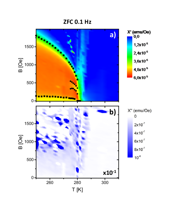
Figure 1: a Contour plots for $\chi^{\prime}$ b and $\chi^{\prime\prime}$ for a frequency of $0.1$ Hz (decreasing magnetic field). The black squares indicate the phase boundaries.

3 Determination of relaxation times

At the conical to helical transition ($H_{c1}$) close to the transition temperature (270 - 280 K) an increasing signal in $\chi^{\prime\prime}$ is seen in the 5 Hz phase diagram. To determine the relaxation times, we simultaneously analyse $\chi^{\prime}$ and $\chi^{\prime\prime}$ by the modified Cole-Cole formalism [10, 9] ($\chi^{\prime}$ and $\chi^{\prime\prime}$ are connected by the Kramers-Kronig relation, therefore reasonable values can only be found by analysing them together [11]).

Modified Cole-Cole formalism:

$$\chi(\omega)=\chi(\infty)+\frac{\chi(0)-\chi(\infty)}{1+(i\omega\tau_{0})^{1-\alpha}}$$ (1)

$\chi(0)$ and $\chi(\infty)$ are the isothermal and adiabatic susceptibilities; $\omega$ is the angular frequency; and $\tau_{0}$ is the characteristic relaxation time. $\alpha$ is a parameter that defines the width of the relaxation frequencies distribution. $\alpha=0$ corresponds to one single relaxation process and $\alpha=1$ accounts for an infinitely broad relaxation distribution. The equation can be separated into a real and imaginary part:

$$\chi^{\prime}(\omega)=\chi(\infty)+\frac{A_{0}[1+(i\omega\tau_{0})^{1-\alpha}\sin(\pi\alpha/2)]}{1+2(\omega\tau_{0})^{1-\alpha}\sin(\pi\alpha/2)+(\omega\tau_{0})^{2(1-\alpha)}}$$ (2)

$$\chi^{\prime\prime}(\omega)=\frac{A_{0}(i\omega\tau_{0})^{1-\alpha}\cos(\pi\alpha/2)}{1+2(\omega\tau_{0})^{1-\alpha}\sin(\pi\alpha/2)+(\omega\tau_{0})^{2(1-\alpha)}}$$ (3)

with $A_{0}=\chi(0)-\chi(\infty)$. The equations can be fitted to our frequency data that was acquired along the helical to conical phase transition. An example can be seen in Fig. 2a. All relaxation time values as well as $\alpha$ can be seen in Fig. 2b-c. Most of the relaxation times vary between 0.01 s to 0.2 s and $\alpha$ ranges from 0.3 to 0.8. The real and imaginary susceptibility should give the same relaxation times, which is true for almost all temperatures excluding 280 K. This indicates that our Squid measurements are reliable and determine the macroscopic relaxation times. All $\alpha$ values are between 0-1 indicating that several relaxation processes are happening at this phase transition.

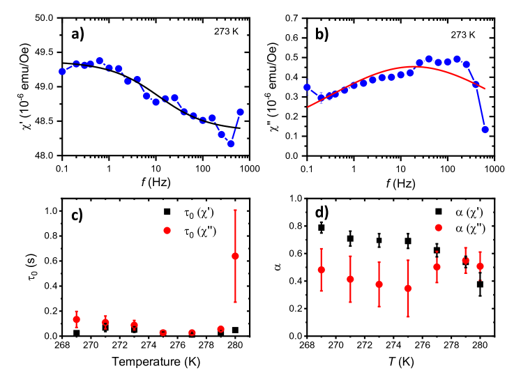
Figure 2: Fitting of the real a and imaginary b frequency-dependent susceptibility at 273 K and under 10 mT. c Relaxation times and d $\alpha$ determined by fitting the frequency dependent Squid measurements along the helical to conical phase transition (280 K/4 mT; 279 K/6 mT; 277 K/8 mT; 275 K/9 mT; 273 K/10 mT; 271 K/11 mT; 269 K/11.5 mT).

References

M. Richardson, P. Kierkegaard, J. Santesson, P. Holmberg, G. Eriksson, R. Blinc, S. Paus̆ak, L. Ehrenberg, and J. Dumanović, Crystal Structure Refinements of the B20 and Monoclinic (CoGe-type) Polymorphs of FeGe, Acta Chem. Scand 21, 753–760 (1967).

B Lebech, J Bernhard & T Freltoftt Magnetic structures of cubic FeGe studied by small-angle neutron scattering. J. Phys.: Condens. Matter 1, 6105-6155 (1989).

A. Dussaux et al., Local dynamics of topological magnetic defects in the itinerant helimagnet FeGe, Nat. Commun. 7, 12430 (2016).

H. Wilhelm, M. Baenitz, M. Schmidt, U. K. Rößler, A. A. Leonov, and A. N. Bogdanov, Precursor Phenomena at the Magnetic Ordering of the Cubic Helimagnet FeGe, PRL 107, 127203 (2011).

A. Vansteenkiste, J. Leliaert, M. Dvornik, M. Helsen, F. Garcia-Sanchez, and B. Van Waeyenberge, The design and verification of MuMax3, AIP Adv. 4, 107133 (2014).

M. Beg, R. Carey, W. Wang, D. Cortés-Ortuño, M. Vousden, M.-A. Bisotti, M. Albert, D. Chernyshenko, O. Hovorka, R. L. Stamps, H. Fangohr, Ground state search, hysteretic behaviour and reversal mechanism of skyrmionic textures in confined helimagnetic nanostructures, Sci. Rep. 5, 17137 (2015).

F. Qian, H. Wilhelm, A. Aqeel, T. T. M. Palstra, A. J. E. Lefering, E. H. Brück, and C. Pappas, Phase diagram and magnetic relaxation phenomena in Cu₂OSeO₃, Phys. Rev. B 94, 064418 (2016).

L. J. Bannenberg, A. J. E. Lefering, K. Kakurai, Y. Onose, Y. Endoh, Y. Tokura, and C. Pappas, Magnetic relaxation phenomena in the chiral magnet ${\mathrm{Fe}}_{1-x}{\mathrm{Co}}_{x}\mathrm{Si}$: An ac susceptibility study, Phys. Rev. B 94, 134433 (2016).

Á. Butykai, S. Bordács, L- F. Kiss, B. G. Szigeti, V. Tsurkan, A. Loidl, and I Kézsmárki, Relaxation dynamics of modulated magnetic phases in the skyrmion host GaV₄S₈: An ac magnetic susceptibility study. Phys. Rev. B 96, 104430 (2017).